
Submitted:
01 May 2025
Posted:
02 May 2025
You are already at the latest version
Abstract
The complexity of land types and the limited spatial resolution of Synthetic Aperture Radar (SAR) imagery have led to the widespread presence of mixed pixels in radar backscatter images. The signal mixture of Endmembers within mixed pixels hinders the establishment of accurate relationships between pure Endmember’s parameters and the corresponding backscatter coefficient, thereby significantly reducing the accuracy of surface parameter inversion. However, few studies focused on decomposing and estimating the pure backscatter signals within mixed pixels. This paper proposes a novel approach based on hyperspectral unmixing techniques and the microwave backscatter contribution decomposition model to estimate the pure backscatter coefficients of all Endmembers within mixed pixels. Experimental results demonstrate that the proposed method can relatively accurately estimate the backscatter coefficients of all end members of mixed pixels. For mixed pixels composed of grassland and soil in the test area, the proportion of pixels with a relative error within 20% in estimating soil and grass endmember backscattering coefficients was close to 80% of the total number of tested pixels. Furthermore, the spatial distribution of the estimated Endmember backscattering coefficients exhibited a high degree of consistency with the endmember types, structures, and conditions that influence their backscattering behavior.
Keywords:
endmembers
; hyperspectral unmixing
; microwave backscatter contribution decomposition model
; radar backscattering coefficient
1. Introduction
Since the 1960s, SAR has been utilized for Earth observation. Today, remote sensing radar has become a standard tool, with its applications steadily expanding into various fields. These include tectonic and lithological mapping in geology[1]. Soil moisture estimation, watershed delineation, flood mapping, surface water, and snow monitoring in hydrology[2,3,4,5]. Crop mapping, growth and harvest monitoring, stress detection, and water resource assessment in agriculture[6,7]. Deforestation monitoring, wildfire damage assessment, and vegetation density estimation in forestry[8,9,10,11]. Topographic mapping, land use classification, landmark change detection, and urban development monitoring in cartography[12,13,14]. And sea ice monitoring, iceberg detection and tracking, glacier and ice sheet mapping, and glacier dynamics observation in polar research[15,16,17]. Unfortunately, most of the aforementioned applications based on radar backscatter coefficients suffer from mixed-pixel signals. The signal mixture makes it difficult to establish a reliable relationship between the surface target’s pure backscatter response and its associated biophysical parameters, thereby limiting the accuracy of parameter retrieval.
There is limited research on the decomposition and estimation of backscattered power from endmembers within mixed pixels. Among the limited related studies, polarimetric decomposition of the backscatter matrix is one of the few approaches that address this issue. This technique decomposes the backscattering matrix into surface scattering, volume scattering, and double-bounce scattering components, thereby providing insights into the types of endmembers contributing to the observed backscattered energy.
Methods for polarimetric scattering decomposition can be broadly categorized into three types. The first type, proposed by Freeman and Durden based on the assumption of reflection symmetry, decomposes the polarimetric SAR backscatter matrix into a linear combination of volume scattering, surface scattering, and double-bounce scattering. Using fully polarimetric SAR observations, the scattering powers of these three components are estimated, which in turn characterize the earth's surface target and its parameters [18]. Yamaguchi introduced a helix scattering term into the model, expanding the scattering mechanisms from three to four categories, thereby enhancing the model's ability to describe complex high-scattering targets[19]. Shubham replaced Volume Power with Depolarized Volume Power (DVP) and Anisotropic Volume Power (AVP) to improve polarization's sensitivity to vegetation scattering. Although this approach can enhance the accuracy of Leaf Area Index (LAI) inversion to some extent, it cannot fundamentally distinguish the volume scattering contributions of different endmembers within mixed pixels[20]. Ainsworth proposes a new approach to solve model-based decomposition by employing an L1-regularized optimization procedure, which automatically selects a set of optimal polarimetric scattering mechanisms and guarantees nonnegative powers for the selected scattering mechanisms[21]. Progress in this category of methods has been modest, with current research primarily aimed at refining internal scattering models to improve the accuracy of scattering power estimates for individual scattering mechanisms. However, these approaches remain inadequate in estimating endmember-specific scattering powers within mixed pixels. The second category is represented by the method proposed by Cloude and Pottier, which is entirely based on eigenvector decomposition. This approach decomposes the backscattering matrix into entropy, anisotropy, and alpha angle to characterize different scattering mechanisms. Through this decomposition, the dominant scattering mechanism and the associated scattering power can be inferred from the principal eigenvalue and its corresponding eigenvector[22]. Mott made approximations to interpret the eigenvector-based decomposition results regarding known scattering mechanisms [23]. Although these methods can identify the dominant scattering mechanism within mixed pixels, they remain insufficient for resolving the backscattered power contributions of individual endmembers.
In our study on desertification in arid and semi-arid regions, we proposed the microwave backscattering contributions decomposition (MBCD) model within mixed pixels containing only two endmembers: soil and vegetation. Additionally, we developed a buffer-based approach for estimating the backscattering coefficients of individual endmembers [24]. The buffer-based approach for estimating endmember backscattering coefficients requires endmember abundances within mixed pixels as prior information. In our previous work, vegetation abundance was derived using the vegetation coverage method, and soil abundance was indirectly inferred. However, this approach becomes inadequate when mixed pixels contain three or more endmembers, as it cannot retrieve the abundances of all endmembers. Therefore, this study proposes integrating hyperspectral unmixing techniques to provide an abundance of information for endmember backscattering coefficient estimation. Combining hyperspectral unmixing with the buffer-based estimation approach makes it possible to estimate the backscattering coefficients of individual endmembers within arbitrarily complex mixed pixels.
Current methods for extracting pure endmembers from hyperspectral imagery can be broadly classified into four categories: spectral library-based, visual interpretation, geometrical approaches, and deep learning-based techniques[25,26,27,28,29,30,31,32,33].
Visual interpretation relies on prior knowledge of the ground surface’s spectral characteristics and textures in optical imagery, allowing users to select representative pixels as pure endmembers manually. Among geometrical approaches, the N-FINDR algorithm and its variants are the most representative[34]. These algorithms are based on the assumption that end members form a simplex of maximum volume in the feature space. By identifying the set of pixels that define this maximum-volume simplex, the algorithms aim to extract pure endmembers from the hyperspectral data. Another classical geometrical method is the Pixel Purity Index (PPI)[35]. This method is based on projection analysis, where image pixels are projected onto many random vectors. The frequency with which a pixel appears at the extremes of these projections is recorded, with pixels appearing most frequently at extreme positions considered more likely to represent pure endmembers. In recent years, with the advancement of deep learning techniques and the increasing availability of labeled samples, deep learning has been gradually applied to endmember extraction and has demonstrated relatively promising performance[36,37,38,39,40].
Commonly used spectral unmixing methods can be broadly categorized into two main types: Physics-Based and Data-Driven spectral unmixing[41]. Data-driven hyperspectral unmixing methods aim to directly learn the mapping between endmember spectra and abundances from observed data without relying on predefined physical models or spectral assumptions[42,43,44]. Physics-based spectral unmixing methods interpret the composition and proportions of mixed pixels by constructing mathematical models grounded in physical laws that govern the interactions between light and matter[45,46,47,48]. Data-driven hyperspectral unmixing methods rely heavily on large volumes of high-quality training data and may exhibit limited generalization capability when faced with high-dimensional features, noise, or significant endmember variability. Physically-based nonlinear spectral unmixing methods can more accurately model complex interactions among surface materials; however, their high model complexity and difficulty in parameter estimation often result in greater uncertainty in the derived abundance estimates. In contrast, linear models offer a simpler structure and clearer physical interpretability, making them suitable for most practical applications and thus widely adopted.
Therefore, this study proposes a general technical framework for estimating endmember-level backscattering coefficients within mixed pixels by integrating linear hyperspectral unmixing with the MBCD model. The main objective of this work is to validate and evaluate the proposed framework to determine whether the resulting accuracy meets the requirements for practical applications.
2. Data and Methods
2.1. Test Area
The selection of the test area primarily depends on the availability of hyperspectral data. Although numerous open-access hyperspectral datasets are currently available, most of them are designed for tasks such as spectral unmixing or land cover classification and often lack corresponding spatial location information. Considering the completeness of geolocation, the complexity of land cover types, and computational demands (as hyperspectral datasets usually contain hundreds of spectral bands), we finally selected a region within Yellowstone National Park as the test site. This area covers approximately 1.67 square kilometers, as shown in Figure 1.
YELL highly represents a wildland area in the National Ecological Observatory Network (NEON) 's Northern Rockies Domain. The terrain consists of rolling hills spanning 1840 - 2245 m (6036 - 7360 ft.) in elevation at the site. The site is a mosaic of pine-dominated forest mixed with open swaths of sage, grass, and small wetlands. Soils at the YELL NEON site fall into the Molli soil category. Most soils found in the area are within loamy-skeletal particle-size families. The most common soil type found in the NEON sample plots was Hobacker gravelly loam[49].
2.2. Datasets
2.2.1. Hyperspectral Data
In this study, we utilized hyperspectral imagery provided by the NEON, specifically the Surface Bidirectional Reflectance data product acquired through the NEON Airborne Observation Platform (AOP). This dataset is derived from visible to shortwave infrared (VSWIR) hyperspectral imagery, spanning a spectral range from approximately 380 nm to 2510 nm. It consists of 426 spectral bands with a resolution of approximately 5 nm, and the reflectance values are scaled by a factor of 10,000. Wavelength regions corresponding to strong water vapor absorption, namely 1340–1445 nm and 1790–1955 nm, are masked out and assigned a value of -100 due to the lack of valid reflectance information. Additionally, the dataset includes quality assurance (QA) raster bands to assist in the filtering of unreliable observations. The dataset underwent a series of preprocessing steps to ensure geometric and radiometric accuracy, including orthorectification and corrections for atmospheric effects, topography, and Bidirectional Reflectance Distribution Function (BRDF). The final reflectance mosaic was constructed using nadir-most pixels from flight lines with minimal cloud cover. Hyperspectral data of the test area, acquired on July 4, 2023, were obtained from the Google Earth Engine (GEE) platform and exported to the local disk for subsequent processing.
2.2.2. Microwave Backscatter Data
Microwave backscatter data were obtained from the Sentinel-1A mission, which carries a C-band SAR instrument operating at 5.405 GHz. The Ground Range Detected (GRD) products were preprocessed using the Sentinel-1 Toolbox to generate terrain-corrected and radiometrically calibrated backscatter data. The preprocessing pipe-line included thermal noise removal, radiometric calibration, and terrain correction based on the Shuttle Radar Topography Mission (SRTM) 30 m Digital Elevation Model (DEM), or ASTER DEM in high-latitude regions where SRTM is unavailable. The resulting backscatter coefficients were converted to decibel (dB) values using a logarithmic scale transformation. This study used GRD products acquired in the ascending orbit mode with single-polarization VV (vertical transmit and receive). The data of the test area, acquired on July 4, 2023, was retrieved through the GEE platform.
2.3. Methods
2.3.1. A General Technical Framework for Estimating the Backscatter Coefficients of Endmembers within Mixed Pixels
Figure 2 illustrates the overall technical framework for estimating endmember backscatter coefficients in mixed pixels proposed in this study. Building upon our previous work, we first extend the two-endmember MBCD model to a multiply-endmember MBCD model. This extension is derived through rigorous theoretical analysis, resulting in a backscatter energy conservation Equation applicable to arbitrary mixed pixels. This Equation forms the theoretical foundation for the estimation of endmember backscatter coefficients.
Secondly, we continued to employ the "buffer-based estimation approach" proposed in our previous work, assuming that end members of the same class within a buffer share identical backscatter coefficients; this approach remains applicable in the case of multiple members. Based on the multi-endmember MBCD model, an energy conservation Equation can be established for each mixed pixel within the buffer. Since the abundance of the same end member is usually different across different mixed pixels in the buffer, it becomes possible to construct a system of energy conservation Equations encompassing all mixed pixels within the buffer zone.
Finally, singular value decomposition (SVD) is applied to the abundance matrix to obtain a least-squares estimate of the endmember backscatter coefficient vector for mixed pixels. When two mixed pixels within the buffer exhibit highly similar endmember types and abundances, the abundance matrix may become singular, leading to low estimation accuracy. SVD helps mitigate this issue by improving the solution's numerical stability and computational efficiency.
2.3.2. Acquisition of Pure Endmember and Corresponding Spectral Features
Given the relatively small spatial extent of the study area, the low spectral-spatial variability among similar endmembers, and the limited number of pure pixels, traditional methods such as PPI and N-FINDR may fail to accurately identify pure pixels due to their sensitivity to threshold settings. To address this issue, we adopted a method based on visual interpretation in combination with the Normalized Difference Vegetation Index (NDVI) to identify pure pixels and extract their representative spectral signatures.
The specific procedure is as follows:
(1) NDVI values were extracted for the study area and subjected to density segmentation. (2) Pure Tree and grass pixels were identified by iteratively adjusting the NDVI threshold range. Theoretically, a larger vegetative cover corresponds to higher chlorophyll content and, thus, higher NDVI values. Candidate regions for Tree and grass were first visually identified using high-resolution imagery, after which a lower NDVI threshold was applied to isolate spectrally pure Tree and grass pixels. (3) Pure soil endmembers were determined using the upper NDVI threshold. In theory, chlorophyll content decreases as the soil fraction increases, resulting in lower NDVI values. Visually identifiable pure soil regions were used as a reference, and an appropriate upper NDVI limit was applied to extract pure soil pixels. (4) Roads within the study area are primarily composed of cement and exhibit distinct spectral characteristics, allowing pure road pixels to be visually identified from the RGB imagery.
2.3.3. Fully Constrained Least Squares (FCLS) Spectral Unmixing Model
Considering the complexity of nonlinear spectral unmixing models and the scarcity of ground-truth abundance data required for training deep learning-based unmixing approaches, this study employs the classical FCLS method to perform hyperspectral unmixing and retrieve endmember abundance information. The FCLS algorithm was originally proposed by Heinz in 2001, and This method assumes that the observed spectrum of a given pixel can be expressed as a linear combination of endmember spectra[45]:
Here, is an vector representing the reflectance of a mixed pixel across N spectral bands; M is an N×p matrix corresponding to the reflectance spectra of p endmembers; α is a p×1 vector denoting the abundance of the endmembers within the mixed pixel; is an N×1 vector representing the noise. Therefore, the estimation of endmember abundances in a mixed pixel can be expressed as:
2.3.4. Development of the MBCD Model
Assume that the total area of a mixed pixel is , which contains M types of endmembers. The area occupied by the i-th endmember is denoted as . The backscatter coefficient of this mixed pixel is denoted by , while represents the backscatter coefficient of the i-th endmember to be estimated, where i is a positive integer ranging from 1 to M. It is assumed that a total of N mixed pixels within the buffer zone are used to estimate the endmember backscatter coefficients. According to the definition of the backscatter coefficient, the backscatter coefficient of the mixed pixel can be expressed as the ratio of the backscattered power to the incident power.
In the above Equation 3, denotes the backscattered power, represents the incident power, and σ is the backscatter coefficient of this mixed pixel. By performing a straightforward transformation of the Equation 3, the backscattered power of this pixel can be expressed as follows:
Similarly, the backscattered power of the i-th endmember within this mixed pixel can be expressed as follows:
Therefore, the backscattered energy of this mixed pixel can be derived from two different perspectives, which, according to the law of energy conservation, should be equal:
In the above Equation 6, the left side represents the total backscattered energy of the mixed pixel, obtained by multiplying the backscatter power by the pixel area. The right side denotes the sum of the backscattered energies contributed by all endmembers within the mixed pixel, representing the total backscattered energy. According to the principle of energy conservation, the physical quantities on both sides of Equation 6 are equivalent and must be equal.
By replacing the backscattered power in Equation (6) with the incident power, we obtain the following Equation:
The incident power on both sides of Equation 7 can be canceled out, resulting in a simplified energy conservation Equation for the mixed pixel:
In the above Equation, represents the ratio of the area occupied by the i-th endmember to the total area of the pixel, which corresponds to the abundance of endmember i. By denoting , the final energy conservation Equation for the mixed pixel can be expressed as:
The energy conservation Equation (Equation 9) enables the decomposition of backscatter contributions from multiple endmembers within a mixed pixel and will serve as the fundamental basis for estimating endmember backscatter coefficients within mixed pixels.
2.3.5. Sub-Pixel-Level Backscattering Contributions Estimation
The key factors determining endmembers' backscatter coefficient include the endmembers' type, structure, and condition. For natural, spatially adjacent, non-manmade targets (such as soil, trees, or grass), the variations in the factors affecting backscatter (such as the composition, structure, and growth condition of vegetation) are typically small. Similarly, for artificial targets in a natural environment that are spatially adjacent (such as buildings or cement roads), the factors influencing the backscatter (such as the material composition and structure of buildings and roads) usually exhibit minor variations. Therefore, it can be assumed that endmembers of the same type within spatially adjacent mixed pixels share the same backscatter coefficient. Based on this assumption, this study proposes a method for estimating the backscatter coefficients of endmembers within mixed pixels.
A buffer zone with a radius of R is established around the mixed pixel P to be estimated (the buffer radius is chosen to ensure that the composition, structure, and condition of the same type of endmembers within the buffer do not exhibit significant spatial variation). It is assumed that there are N mixed pixels within the buffer, with the backscatter coefficient of the j-th mixed pixel denoted as , where j is a positive integer ranging from 1 to N. Furthermore, each pixel contains M types of endmembers, and the backscatter coefficient of the i-th endmember is denoted as , where i is a positive integer ranging from 1 to M. Based on Equation 6, a system of linear unmixing Equations for estimating the backscatter coefficients of endmembers within the mixed pixel P can be constructed:
For any mixed pixel j within the buffer zone of the mixed pixel P, the abundance of endmember , denoted as , can be estimated using the linear spectral unmixing model described in Section 2.3.2. Meanwhile, the backscatter coefficient of mixed pixel j can be directly obtained from the original radar imagery. Therefore, the only unknowns in the system of Equations (10) are the backscatter coefficients of the endmembers within the target mixed pixel P, namely σ₁, σ₂, ..., . To facilitate the formulation and solution of Equation (10), we introduce the following notations for its variables:
The matrix F contains the abundances of all endmembers within the N pixels in the buffer zone and is referred to as the abundance matrix of the buffer. The vector b includes the composite backscatter coefficients of these N mixed pixels and is termed the composite backscatter vector. The vector X, which consists of the backscatter coefficients of all endmembers within the target mixed pixel P, is the unknown endmember backscatter coefficient vector. Based on these definitions, the system of Equation 11 can be concisely written as:
When two or more mixed pixels within the buffer zone exhibit similar endmember abundance distributions, this may lead to linear dependence among two or more row vectors in the abundance matrix F, thereby preventing the accurate computation of a least squares solution. In such cases, SVD can be applied to the matrix F. The SVD of the abundance matrix F can be expressed as:
Based on the singular value decomposition of F, the least squares estimate can be expressed as:
where denotes the first columns of .
2.3.6. Verification Scheme of Backscattering Contributions Estimation
Direct field measurements of endmember backscattering coefficients are often impractical. Therefore, we propose a relatively simple approach to validate the accuracy of the estimated endmember backscattering coefficients. Taking a mixed pixel composed of soil and grass endmembers as an example, we use the backscattering power of pure soil and grass pixel regions within the buffer zone to approximate the true backscattering coefficients of soil and grass endmembers in the target mixed pixel P as illustrated in Figure 2. Assuming that the buffer zone centered on the target pixel contains N mixed pixels for estimating the endmember backscattering coefficients, and that each mixed pixel has an equal area s, the following relationship holds:
Therefore, for mixed pixels composed solely of soil and grass endmembers, the true values of the endmember backscattering coefficients can be approximated as:
The estimation error of the backscattering coefficient is quantified using relative error:
3. Results
3.1. Pure Endmember Extraction
Pure endmembers were extracted based on visual interpretation and NDVI values, following the procedure outlined in Section 2.3.1. Specifically, the NDVI range for pure tree endmembers was defined as (0.9600, 1.0000), for pure grass endmembers as (0.8300, 0.8500), and pure soil endmembers as (0.0586, 0.1500). Pure road endmembers were extracted primarily based on visual interpretation, with NDVI values set below 0.1. The results of the extraction for each pure endmember type are presented in Figure 3.
3.2. Pure Endmember Spectral Features
Based on the four types of pure endmember regions of interest identified in Section 3.1, the spectral signature curves of each class were derived by averaging the reflectance values across all corresponding pure pixels. As shown in Figure 4, the four classes exhibit distinct spectral characteristics. In the visible wavelength range (400–700 nm), roads show the highest reflectance, followed by soil, grass, and trees. This pattern aligns with the visual impression from the true-color image in Figure 1, where roads appear the brightest, followed by soil, grass, and trees. The relatively low reflectance of trees may be attributed to shadow effects. The consistency between the visual appearance in the visible spectrum and the derived spectral curves supports the reliability and accuracy of the extracted spectral signatures for the four pure endmember types.
3.3. Abundance of Pure End Members
Based on the spectral signature curves of the four endmember types extracted in Step 3.1, we applied the FCLS hyperspectral unmixing method to the hyperspectral imagery of the test area, and the abundance maps for the four endmembers were generated for the study region.
Figure 5.
Abundance maps of the four endmembers in the test area.
The accuracy of abundance estimation for mixed pixels is critical for the subsequent estimation of endmember backscattering coefficients. Therefore, it is essential to evaluate the abundance of unmixing results. However, since ground truth data on actual endmember abundances are not available for the selected study area, we assess the accuracy of the estimated abundances using both the root mean square error (RMSE) from the unmixing process and visual inspection. The RMSE, which is commonly used to evaluate spectral unmixing performance, is defined as follows:
In Equation 21, represents the reflectance of the mixed pixel at the ith spectral band, while denotes the reconstructed reflectance at the same band, obtained by the estimated endmember abundances and the endmember spectral matrix. A smaller RMS indicates better performance in reconstructing the mixed pixel’s spectrum using the estimated abundances, implying lower reconstruction error. Conversely, a larger RMS suggests that the pixel may not fully conform to the linear mixing model or that the endmember extraction may be insufficient or inaccurate. The RMS error distribution of hyperspectral unmixing is illustrated in Figure 6.
3.4. Endmember Backscattering Coefficient
For any mixed pixel, when the abundance of an endmember approaches 1, the contributions of the other end members become negligible. In such cases, the backscattering energy of the pixel is likely dominated by this single endmember, which can be treated as a pure pixel. The backscattering coefficient of this mixed pixel will be viewed as that of the endmember, and the backscattering coefficients of the other endmembers are assigned as nan. Additionally, in special cases—such as a mixed pixel primarily composed of grass that contains an uncovered strong scatterer or a high-scattering region—the backscattering coefficient of the grass endmember may be significantly overestimated. This issue can be mitigated by applying a spatial median filter to the backscattering coefficient. If estimation is forced under such conditions, the extremely low abundance values of other endmembers may lead to instability and unreliability in the solution of Equation 12. Therefore, during the estimation of endmember backscattering coefficients, a lower bound threshold is imposed on the endmember abundances in Equation 12. When the abundance of any endmember falls below 0.05, the resulting unmixing error can be substantial. Hence, any endmember with an abundance below this threshold within a mixed pixel is considered absent, and its backscattering coefficient is marked as invalid during the estimation process. This study adopts a threshold of 0.9 for endmember abundance to identify pure pixels, which means pixels with endmember abundances greater than 0.9 are regarded as pure pixels. The estimation results of endmember backscattering coefficients for different types of mixed pixels are shown in Figure 7. It should be noted that for the outermost 5 rows and 5 columns of the hyperspectral image in the test area, a 9×9 buffer could not be constructed. As a result, the endmember backscattering coefficients for the mixed pixels in these boundary regions were not estimated. Instead, their values were uniformly set to zero.
3.4. Endmember Types of the Test Area
Prior to validation, it is essential to understand the types and spatial distribution of mixed pixels within the entire test area. To this end, we classified and encoded the mixed pixels. Based on the number of endmembers present in each pixel, the mixed pixels were categorized into four major groups: those containing 1, 2, 3, or 4 endmember types. Specifically, the number of possible combinations for each group is given by the binomial coefficients: for pixels with 1 endmember type, for 2 types, for 3 types, and for 4 types, resulting in a total of 15 distinct mixed pixel types. We summarized the number and proportion of each of these 15 types (Table 1) and visualized their spatial distribution across the study area (Figure 8).
As shown in Table 1, the mixed pixel types in the test area are primarily concentrated in Types 1, 4, 8, and 12. Among them, the most prevalent type is the mixture of soil and grass, which accounts for approximately 50% of the study area. Pure grass pixels constitute the second largest category, occupying approximately 27% of the area, while mixed pixels containing soil, grass, and trees cover more than 13% of the area. The remaining mixed pixel types are rare, each contributing less than 5% of the total area. According to the spatial distribution illustrated in Figure 8, mixed pixels' types and distribution patterns are highly consistent with the land cover patterns shown in Figure 1. For example, pure grass pixels are mainly distributed in areas with higher grass coverage, whereas pixels containing both soil and grass are found in regions with lower grass density and partial soil exposure.
Considering that the validation process requires the buffer zone of the target mixed pixel to include pure pixels of all endmember types present in the mixed pixel itself, only Types 4 and 12—both involving at least two endmember classes and accounting for more than 5% of the study area—were eligible for evaluation. However, the surrounding pure pixels of soil, grass, and trees in the vicinity of Type 12 are not ideally interlaced in space. Therefore, Type 4 mixed pixels were selected to validate the accuracy of estimated endmember backscatter coefficients.
3.5. Verification of the Estimated End-Member Backscattering Coefficients
Due to the random spatial distribution of pure soil and grass pixels within the buffer zones of Type 4 mixed pixels, not all such pixels are suitable for validation. If the number of pure pixels corresponding to any endmember within the buffer falls below a certain threshold, random noise may render the backscatter coefficient of pure pixel unreliable as a representative of the endmember’s true backscatter response within the mixed pixel. Therefore, during the validation process, we first counted the number of pure soil and grass pixels within a 9×9 buffer around each Type 4 mixed pixel. Only those mixed pixels whose buffer zones contained more than five pure pixels for both soil and grass were selected to assess the estimated endmember backscatter coefficients accurately. For the selected pixels, relative errors were calculated, followed by a preliminary statistical analysis. The results are presented in Figure 9.
For the estimation results of soil backscatter coefficients within the mixed pixels, 54.22% of the pixels exhibited relative errors within the range of 0–10%, 24.42% within 10–20%, and 10.05% within 20–30%. The proportions of pixels with relative errors in 30–40%, 40–50%, and 50–100% were 4.13%, 2.33%, and 4.85%, respectively. These results indicate that the proportion of the area with relative errors exceeding 50% was less than 5%.
For the estimation of grass backscatter coefficients, 55.63% of the pixels had relative errors within 0–10%, 21.52% within 10–20%, and 10.76% within 20–30%. The corresponding proportions for the 30–40%, 40–50%, and 50–100% ranges were 3.48%, 4.14%, and 4.47%, respectively, indicating that the area proportion with relative errors greater than 50% remained below 5%.
4. Discussion
4.1. Accuracy of Endmember Abundance Estimation
The accuracy of endmember abundance estimation was evaluated from both qualitative and quantitative perspectives. Overall, the spatial distributions of soil, grass, road, and tree abundances in the abundance maps (Figure 5) show a high degree of consistency with the distributions of these land cover types in Figure 1. Apart from artificial objects, the environmental parameters of natural soils that influence vegetation growth typically exhibit gentle and continuous spatial variations. Consequently, the biomass supported by the soil also varies gently and continuously across space, implying that vegetation cover should not experience drastic spatial changes; rather, it is expected to vary similarly and continuously. For each endmember (soil, grass, or tree) abundance map, the spatial continuity of the abundance values corresponds well to the expected continuity of the associated endmember cover fraction. In particular, the bright areas in the abundance maps (Figure 5) closely match regions with higher coverage of the corresponding land cover types in Figure 1.
To quantitatively evaluate the accuracy of endmember abundance estimation in this study, we conducted an extensive review of literature related to hyperspectral unmixing. The results of this review indicate that, when applied to the same hyper-spectral dataset, deep learning-based unmixing methods generally outperform the FCLS method used in this study. However, the accuracy of the FCLS method largely depends on the selection of pure endmember spectral signatures. By adopting a novel approach that combines visual interpretation with NDVI-based density segmentation, the RMSE of hyperspectral unmixing achieved in this study, while slightly lower than that of deep learning methods, is nonetheless very close to that of deep learning methods, which demonstrates that the endmember abundance results derived from hyperspectral unmixing in this study are reliable(Figure 6)[50,51,52,53].
4.2. Evaluation of Endmember Backscattering Coefficient Estimation
We evaluated the proposed framework's performance in estimating endmember backscattering coefficients in mixed pixels from both qualitative and quantitative perspectives.
As shown in Figure 7(a), when soil abundance is lower than 5%, its backscattering coefficient is set to nan value. The soil backscattering coefficients across most grass-covered areas are relatively low, while a significant increase is observed in areas adjacent to trees, which is likely because the soils near trees possess higher moisture and inorganic salt content compared to soils in grassland areas, leading to a notable increase in their backscattering coefficients. Trees generally require more water and nutrients for growth than grasses, which supports the observed spatial distribution of the soil backscattering coefficients. Moreover, the estimated soil backscattering coefficients exhibit good spatial continuity, meaning their variations across space are relatively gentle, which is consistent with the spatial distribution patterns of soil properties, such as type and condition that govern the backscattering behavior. These results demonstrate that the estimated soil backscattering coefficients possess good spatial consistency and are physically reasonable.
Due to mixed pixel types that do not contain grass endmembers (types 0, 2, 3, 5, 6, and 11), there are invalid values regions in the grass backscattering coefficients map, as shown in Figure 7b. By carefully checking the spatial distribution of grass endmember backscattering coefficients in Figure 7b, it can be observed that most areas containing grass endmembers exhibit relatively low backscattering coefficients. In regions where tree endmembers are also present (as shown in Figure 7b and Figure 7d), the grass backscattering coefficients show a moderate increase, although not as pronounced as the increase observed for soil backscattering coefficients. This phenomenon may be attributed to soils near trees having higher moisture and inorganic salt contents than grassland soils, promoting more vigorous grass growth. Consequently, grass's biomass and water content in these areas are slightly higher than in regions without tree endmembers, leading to a moderate increase in the grass backscattering coefficients. Like the spatial distribution of soil backscattering coefficients, the estimated grass backscattering coefficients exhibit good spatial continuity, consistent with the spatial patterns of factors such as grass type, structure, and growth status that influence backscattering behavior. These results indicate that the estimated grass backscattering coefficients also possess good spatial consistency and are physically meaningful.
Since mixed pixels containing roads are usually found at the edges of the roads, a large number of invalid value regions appear in the road's backscattering coefficient map. However, as shown in Figure 7c, some mixed pixels containing road endmembers are still present beside roads, which may be due to the presence of concrete surfaces in the area or soils with similar spectral characteristics to the roads. As expected, the backscattering coefficients across the road area are relatively low, as the road surface is electromagnetically smooth to C-band electromagnetic waves. Most of the energy is reflected specularly, resulting in minimal backscattered energy. So, the low backscattering coefficients are consistent with the geometric properties of the road.
The tree end member is absent for most of the test area, leading to many invalid value regions in the tree backscattering coefficient map. It can be observed that the backscattering coefficients of tree endmembers across the entire study area are generally low, though slightly higher than those of the corresponding grass regions, which is because the biomass and water content of tree endmembers are typically higher than those of grass endmembers, resulting in higher backscattering energy for tree endmembers. Furthermore, the backscattering coefficients are significantly higher in regions with higher tree endmember abundance than those with lower tree endmember abundance, which could be attributed to the denser tree coverage. As trees become dense, tree trunks, branches, and leaves increase, leading to stronger backscattering energy. Consequently, areas with higher tree endmember abundance exhibit relatively higher backscattering energy. Lastly, the continuous spatial distribution of tree endmember backscattering coefficients further indicates that the estimated results have good spatial consistency.
The soil endmember's backscattering coefficient estimation results are relatively ideal from a quantitative perspective. The number of pixels with a relative error within 20% accounts for 78.64% of the total test pixels, while the number of pixels with a relative error within 30% constitutes approximately 88.69% of the test pixels. The number of pixels with a relative error within 40% is around 92.82%, and those with a relative error within 50% make up 95.15% of the total test pixels. Since we use approximately pure soil endmembers to represent the pure soil pixels, these pure soil pixels typically contain a small amount of grass. Given that the backscattering coefficient of the pure grass endmember is generally higher than that of the pure soil endmember (as confirmed through practical testing), the estimation error for the soil backscattering coefficient is slightly higher than the results mentioned above.
The estimation results of the grass endmember backscattering coefficient are slightly lower in accuracy compared to those for soil. The number of pixels with a relative error within 20% accounts for 77.15% of the total test pixels, while the number of pixels with a relative error within 30% constitutes approximately 87.91% of the test pixels. The number of pixels with a relative error within 40% is around 91.39%, and those with a relative error within 50% make up 95.53% of the total test pixels. Since we use approximately pure grass endmembers to represent the pure grass pixels, these pure grass pixels typically contain a small amount of soil. Given that the backscattering coefficient of the pure soil endmember is generally lower than that of the pure grass endmember, the estimation error for the grass backscattering coefficient is slightly lower than the results mentioned above.
Additionally, the buffer size used in this study is 9×9 pixels, with a radius of approximately 45 meters. Although the backscattering characteristics of soil and grass do not change significantly, the end member's backscattering coefficient of this buffer size may not accurately represent the true backscattering coefficients of the endmembers within the center mixed pixel. Therefore, if real endmember backscattering data were available, the estimation accuracy of the endmember backscattering coefficients could potentially be higher.
4.3. Application Prospects and Future Work of This Study
The endmember backscattering coefficients presented with certain relative errors (Figure 7) reveal interesting spatial variation patterns of ground surface targets. For instance, when the spatial distribution of salinity in the test area shows little variation, the terrain is relatively flat, and the surface roughness is similar, the differences in the spatial distribution of soil backscattering coefficients are likely reflective of variations in soil moisture. When the grass type is consistent across the test area, differences in the grass endmember backscattering coefficients reflect spatial variations in grass growth. Similarly, when the tree type is consistent, spatial variations in tree endmember backscattering coefficients indicate differences in tree health or growth.
At the current error level, pure endmember backscattering coefficients for surface parameter inversion and machine learning are yet to be fully assessed. However, the importance of using polarization decomposition-related information for land cover classification has been proved. In the future, efforts will continue to improve model accuracy and test the application of pure endmember backscattering coefficients in surface parameter inversion and machine learning. This ongoing work aims to continually enhance the precision of endmember backscattering coefficient estimation and advance its widespread application across various fields.
Author Contributions
“Conceptualization, Y.S. and H.Z.; methodology, Y.S.; software, Z.Z.; validation, J.W., L.L. and B.S.; formal analysis, H.Z.; investigation, Y.S.; resources, R.T.; data curation, L.Z.; writing—original draft preparation, Z.Z.; writing—review and editing, Y.S.; visualization, L.Z.; supervision, J.L.; project administration, X.G.; funding acquisition, Y.S. All authors have read and agreed to the published version of the manuscript.”
Funding
Please add: This work was supported by the Hebei Province Central Guidance Local Science and Technology Development Fund Project (Grant No. 246Z5402G), the Xinjiang Manas County cultivated land extraction and corn growth monitoring project (Grant No. YG-2025-04-H), the Key Project of North China University of Aerospace Engineering Research Fund (Grant No. ZD-2025-04), the Key R&D Program of Xinjiang Uygur Autonomous Region (2022B03021-1, 2022B03001), the National Natural Science Foundation of China (NSFC-U1803120, E0130105, 42071141, 41877012 and 42230708), the Third Xinjiang Scientific Expedition Program (2022xjkk070101), the “Western Light” Talents Training Program of CAS (grant number 2021-XBQNXZ-012), the Tianshan Talent Training Pro-gram of Xinjiang Uygur Autonomous region (2022TSYCLJ0011), the High-End Foreign Experts Project (2020-2023, G2023046005L), the West Light Foundation of The Chinese Academy of Sciences (No. 2020-XBQNXZ-009), the Science Research Project of Hebei Education Department (Grant No. QN2024113), and The APC was funded by the Hebei Province Central Guidance Local Science and Technology Development Fund Project (Grant No. 246Z5402G).
Data Availability Statement
The data presented in this study are available on request from the corresponding author due to privacy.
Acknowledgments
Thanks to Google Earth Engine and the U.S National Science Foundation's National Ecological Observatory Network for providing the NEON AOP Surface Bidirectional Reflectance data. Thanks to Google Earth Engine for providing the C-band Synthetic Aperture Radar Ground Range Detected data.
Conflicts of Interest
The authors declare no conflicts of interest.
Abbreviations
- The following abbreviations are used in this manuscript:
| SAR | synthetic aperture radar |
| DVP | Depolarized Volume Power |
| AVP | Anisotropic Volume Power |
| LAI | Leaf Area Index |
| PPI | Pixel Purity Index |
| NEON | National Ecological Observatory Network |
| AOP | Airborne Observation Platform |
| VSWIR | visible to shortwave infrared |
| QA | quality assurance |
| BRDF | Bidirectional Reflectance Distribution Function |
| GEE | Google Earth Engine |
| GRD | Ground Range Detected |
| SRTM | Shuttle Radar Topography Mission |
| DEM | Digital Elevation Model |
| dB | decibel |
| SVD | singular value decomposition |
| NDVI | Normalized Difference Vegetation Index |
| FCLS | Fully Constrained Least Squares |
| RMSE | root mean square error |
References
- Zhang, Z.J.; Wang, M.; Qi, Y.J.; Su, X.Q.; Kong, D. Deep Learning-Based Methods for Lithology Classification and Identification in Remote Sensing Images. Ieee Access 2025, 13, 3038–3050. [Google Scholar] [CrossRef]
- Beck, H.E.; Pan, M.; Miralles, D.G.; Reichle, R.H.; Dorigo, W.A.; Hahn, S.; Sheffield, J.; Karthikeyan, L.; Balsamo, G.; Parinussa, R.M.; et al. Evaluation of 18 satellite- and model-based soil moisture products using in situ measurements from 826 sensors. Hydrology and Earth System Sciences 2021, 25, 17–40. [Google Scholar] [CrossRef]
- Souza, W.D.; Reis, L.G.D.; Ruiz-Armenteros, A.M.; Veleda, D.; Neto, A.R.; Fragoso, C.R., Jr.; Cabral, J.; Montenegro, S. Analysis of Environmental and Atmospheric Influences in the Use of SAR and Optical Imagery from Sentinel-1, Landsat-8, and Sentinel-2 in the Operational Monitoring of Reservoir Water Level. Remote Sensing 2022, 14. [Google Scholar] [CrossRef]
- Chen, L.F.; Cai, X.M.; Xing, J.; Li, Z.H.; Zhu, W.; Yuan, Z.H.; Fang, Z.H. Towards transparent deep learning for surface water detection from SAR imagery. International Journal of Applied Earth Observation and Geoinformation 2023, 118. [Google Scholar] [CrossRef]
- Song, H.N.; Wang, B.Y.; Qian, X.J.; Gu, Y.H.; Jin, G.D.; Yang, R. Enhancing Water Extraction for Dual-Polarization SAR Images Based on Adaptive Feature Fusion and Hybrid MLP Network. Ieee Journal of Selected Topics in Applied Earth Observations and Remote Sensing 2025, 18, 6953–6967. [Google Scholar] [CrossRef]
- Adrian, J.; Sagan, V.; Maimaitijiang, M. Sentinel SAR-optical fusion for crop type mapping using deep learning and Google Earth Engine. Isprs Journal of Photogrammetry and Remote Sensing 2021, 175, 215–235. [Google Scholar] [CrossRef]
- Bao, X.; Zhang, R.; Lv, J.C.; Wu, R.Z.; Zhang, H.S.; Chen, J.; Zhang, B.; Ouyang, X.Y.; Liu, G.X. Vegetation descriptors from Sentinel-1 SAR data for crop growth monitoring. Isprs Journal of Photogrammetry and Remote Sensing 2023, 203, 86–114. [Google Scholar] [CrossRef]
- Ferrari, F.; Ferreira, M.P.; Almeida, C.A.; Feitosa, R.Q. Fusing Sentinel-1 and Sentinel-2 Images for Deforestation Detection in the Brazilian Amazon Under Diverse Cloud Conditions. Ieee Geoscience and Remote Sensing Letters 2023, 20. [Google Scholar] [CrossRef]
- Tariq, A.; Shu, H.; Li, Q.T.; Altan, O.; Khan, M.R.; Baqa, M.F.; Lu, L.L. Quantitative Analysis of Forest Fires in Southeastern Australia Using SAR Data. Remote Sensing 2021, 13. [Google Scholar] [CrossRef]
- Bernhard, E.M.; Twele, A.; Martinis, S. The Effect of Vegetation Type and Density on X-Band SAR Backscatter after Forest Fires. Photogrammetrie Fernerkundung Geoinformation 2014, 275–285. [Google Scholar] [CrossRef]
- Svoray, T.; Shoshany, M.; Curran, P.J.; Foody, G.M.; Perevolotsky, A. Relationship between green leaf biomass volumetric density and ERS-2 SAR backscatter of four vegetation formations in the semi-arid zone of Israel. International Journal of Remote Sensing 2001, 22, 1601–1607. [Google Scholar] [CrossRef]
- Wu, Y.H.; Huang, J.; He, X.F.; Luo, Z.C.; Wang, H.H. Coastal Mean Dynamic Topography Recovery Based on Multivariate Objective Analysis by Combining Data from Synthetic Aperture Radar Altimeter. Remote Sensing 2022, 14. [Google Scholar] [CrossRef]
- Solórzano, J.V.; Mas, J.F.; Gao, Y.; Gallardo-Cruz, J.A. Land Use Land Cover Classification with U-Net: Advantages of Combining Sentinel-1 and Sentinel-2 Imagery. Remote Sensing 2021, 13. [Google Scholar] [CrossRef]
- Zhang, X.; Chang, L.; Wang, M.S.; Stein, A. Measuring polycentric urban development with multi-temporal Sentinel-1 SAR imagery: A case study in Shanghai, China. International Journal of Applied Earth Observation and Geoinformation 2023, 121. [Google Scholar] [CrossRef]
- Qiu, Y.J.; Li, X.M.; Busche, T.; Shi, L.J. X- and C-Band SAR Signatures of Sea Ice in the Bohai Sea. Ieee Geoscience and Remote Sensing Letters 2024, 21. [Google Scholar] [CrossRef]
- Shokr, M.; Dabboor, M. Polarimetric SAR Applications of Sea Ice: A Review. Ieee Journal of Selected Topics in Applied Earth Observations and Remote Sensing 2023, 16, 6627–6641. [Google Scholar] [CrossRef]
- Sun, Y.; Ye, Y.F.; Wang, S.Y.; Liu, C.; Chen, Z.Q.; Cheng, X. Evaluation of the AMSR2 Ice Extent at the Arctic Sea Ice Edge Using an SAR-Based Ice Extent Product. Ieee Transactions on Geoscience and Remote Sensing 2023, 61. [Google Scholar] [CrossRef]
- Freeman, A.; Durden, S.L. A three-component scattering model for polarimetric SAR data. Ieee Transactions on Geoscience and Remote Sensing 1998, 36, 963–973. [Google Scholar] [CrossRef]
- Yamaguchi, Y.; Moriyama, T.; Ishido, M.; Yamada, H. Four-component scattering model for polarimetric SAR image decomposition. Ieee Transactions on Geoscience and Remote Sensing 2005, 43, 1699–1706. [Google Scholar] [CrossRef]
- Singh, S.K.; Rajendra, P.; Vivek, T.; and Srivastava, P.K. An improved volume power approach to estimate LAI from optimized dual-polarized SAR decomposition. International Journal of Remote Sensing 2023, 44, 5736–5754. [Google Scholar] [CrossRef]
- Ainsworth, T.L.; Wang, Y.T.; Lee, J.S. Model-Based Polarimetric SAR Decomposition: An <i>L</i><sub>1</sub> Regularization Approach. Ieee Transactions on Geoscience and Remote Sensing 2022, 60. [Google Scholar] [CrossRef]
- Cloude, S.R.; Pottier, E.J.I.t.o.g.; sensing, r. A review of target decomposition theorems in radar polarimetry. 1996, 34, 498-518.
- van Zyl, J. Application of Cloude's target decomposition theorem to polarimetric imaging radar data; SPIE: 1993; Volume 1748.
- Song, Y.; Zheng, H.; Chen, X.; Bao, A.; Lei, J.; Xu, W.; Luo, G.; Guan, Q. Desertification Extraction Based on a Microwave Backscattering Contribution Decomposition Model at the Dry Bottom of the Aral Sea. 2021, 13, 4850.
- Dennison, P.E.; Roberts, D.A. Endmember selection for multiple endmember spectral mixture analysis using endmember average RMSE. Remote Sensing of Environment 2003, 87, 123–135. [Google Scholar] [CrossRef]
- Mehalli, Z.; Zigh, E.; Loukil, A.; Pacha, A.A. A new iterative endmember extraction and spectral matching approach to improve the accuracy of mineral identification and mapping. Signal Image and Video Processing 2025, 19. [Google Scholar] [CrossRef]
- Naik, P.; Polonen, I.; Salmi, P. Blind and endmember guided autoencoder model for unmixing the absorbance spectra of phytoplankton pigments. Scientific reports 2025, 15, 13157. [Google Scholar] [CrossRef] [PubMed]
- Gao, W.; Yang, J.Y.; Zhang, Y.; Akoudad, Y.; Chen, J. SSAF-Net: A Spatial-Spectral Adaptive Fusion Network for Hyperspectral Unmixing With Endmember Variability. Ieee Transactions on Geoscience and Remote Sensing 2025, 63. [Google Scholar] [CrossRef]
- Xiang, S.; Li, X.R.; Chen, S.H. An Endmember-Oriented Transformer Network for Bundle-Based Hyperspectral Unmixing. Ieee Transactions on Geoscience and Remote Sensing 2025, 63. [Google Scholar] [CrossRef]
- Shah, D.; Trivedi, Y.; Bhattacharya, B.; Thakkar, P.; Srivastava, P. Hyperspectral endmember extraction using convexity based purity index. Advances in Space Research 2025, 75, 465–480. [Google Scholar] [CrossRef]
- Wang, L.; Bi, Y.; Wang, W.; Li, J.F. Endmember extraction and abundance estimation algorithm based on double-compressed sampling. Scientific Reports 2024, 14. [Google Scholar] [CrossRef]
- Zhang, T.Q.; Liu, D.S. Estimating fractional vegetation cover from multispectral unmixing modeled with local endmember variability and spatial contextual information. Isprs Journal of Photogrammetry and Remote Sensing 2024, 209, 481–499. [Google Scholar] [CrossRef]
- Wang, Z.; Li, J.Z.; Liu, Y.T.; Xie, F.; Li, P. An Adaptive Surrogate-Assisted Endmember Extraction Framework Based on Intelligent Optimization Algorithms for Hyperspectral Remote Sensing Images. Remote Sensing 2022, 14. [Google Scholar] [CrossRef]
- Winter, M.E. N-FINDR: an algorithm for fast autonomous spectral end-member determination in hyperspectral data. In Proceedings of the Conference on Imaging Spectrometry V, Denver, Co, Jul 19-21, 1999; pp. 266-275.
- Boardman, J.W.; Kruse, F.A.; Environm Res Inst, M. AUTOMATED SPECTRAL ANALYSIS - A GEOLOGICAL EXAMPLE USING AVIRIS DATA, NORTH GRAPEVINE MOUNTAINS, NEVADA. In Proceedings of the 10th Thematic Conference on Geologic Remote Sensing - Exploration, Environment, and Engineering, San Antonio, Tx, May 09-12, 1994; pp. I407-I418.
- Alshahrani, A.A.; Bchir, O.; Ben Ismail, M.M. Autoencoder-Based Hyperspectral Unmixing with Simultaneous Number-of-Endmembers Estimation. 2025, 25, 2592.
- Ozkan, S.; Kaya, B.; Akar, G.B. EndNet: Sparse AutoEncoder Network for Endmember Extraction and Hyperspectral Unmixing. IEEE Transactions on Geoscience and Remote Sensing 2019, 57, 482–496. [Google Scholar] [CrossRef]
- Borsoi, R.A.; Imbiriba, T.; Bermudez, J.C.M.J.I.T.o.C.I. Deep generative endmember modeling: An application to unsupervised spectral unmixing. 2019, 6, 374-384.
- Filippi, A.M.; Archibald, R.; Bhaduri, B.L.; Bright, E.A.J.O.E. Hyperspectral agricultural mapping using support vector machine-based endmember extraction (SVM-BEE). 2009, 17, 23823-23842.
- Alfaro-Mejía, E.; Manian, V.; Ortiz, J.D.; Tokars, R.P.J.F.i.E.S. A blind convolutional deep autoencoder for spectral unmixing of hyperspectral images over waterbodies. 2023, 11, 1229704.
- Bioucas-Dias, J.M.; Plaza, A.; Dobigeon, N.; Parente, M.; Du, Q.; Gader, P.; Chanussot, J.J.I.j.o.s.t.i.a.e.o.; sensing, r. Hyperspectral unmixing overview: Geometrical, statistical, and sparse regression-based approaches. 2012, 5, 354-379.
- Feng, X.-R.; Li, H.-C.; Wang, R.; Du, Q.; Jia, X.; Plaza, A.J.I.J.o.S.T.i.A.E.O.; Sensing, R. Hyperspectral unmixing based on nonnegative matrix factorization: A comprehensive review. 2022, 15, 4414-4436.
- Parente, M.; Iordache, M.-D. Sparse unmixing of hyperspectral data: The legacy of SUnSAL. In Proceedings of the 2021 IEEE International Geoscience and Remote Sensing Symposium IGARSS, 2021; pp. 21-24.
- Jiang, B.; Zhang, C.; Zhong, Y.; Liu, Y.; Zhang, Y.; Wu, X.; Sheng, W. Adaptive collaborative fusion for multi-view semi-supervised classification. Information Fusion 2023, 96, 37–50. [Google Scholar] [CrossRef]
- Heinz, D.C.; Chang, C.I. Fully constrained least squares linear spectral mixture analysis method for material quantification in hyperspectral imagery. Ieee Transactions on Geoscience and Remote Sensing 2001, 39, 529–545. [Google Scholar] [CrossRef]
- Nascimento, J.M.; Dias, J.M.J.I.t.o.G.; Sensing, R. Vertex component analysis: A fast algorithm to unmix hyperspectral data. 2005, 43, 898-910.
- Halimi, A.; Altmann, Y.; Dobigeon, N.; Tourneret, J.Y. Nonlinear Unmixing of Hyperspectral Images Using a Generalized Bilinear Model. Ieee Transactions on Geoscience and Remote Sensing 2011, 49, 4153–4162. [Google Scholar] [CrossRef]
- Qu, Q.; Nasrabadi, N.M.; Tran, T.D. Abundance Estimation for Bilinear Mixture Models via Joint Sparse and Low-Rank Representation. Ieee Transactions on Geoscience and Remote Sensing 2014, 52, 4404–4423. [Google Scholar] [CrossRef]
- National Ecological Observatory, N. Site management and event reporting (DP1.10111.001). 2025.
- Palsson, B.; Ulfarsson, M.O.; Sveinsson, J.R. Convolutional Autoencoder for Spectral Spatial Hyperspectral Unmixing. Ieee Transactions on Geoscience and Remote Sensing 2021, 59, 535–549. [Google Scholar] [CrossRef]
- Hong, D.F.; Gao, L.R.; Yao, J.; Yokoya, N.; Chanussot, J.; Heiden, U.; Zhang, B. Endmember-Guided Unmixing Network (EGU-Net): A General Deep Learning Framework for Self-Supervised Hyperspectral Unmixing. Ieee Transactions on Neural Networks and Learning Systems 2022, 33, 6518–6531. [Google Scholar] [CrossRef]
- Borsoi, R.; Imbiriba, T.; Bermudez, J.C.; Richard, C.; Chanussot, J.; Drumetz, L.; Tourneret, J.Y.; Zare, A.; Jutten, C. Spectral Variability in Hyperspectral Data Unmixing. Ieee Geoscience and Remote Sensing Magazine 2021, 9, 223–270. [Google Scholar] [CrossRef]
- Zhang, S.Q.; Zhang, G.R.; Li, F.; Deng, C.Z.; Wang, S.Q.; Plaza, A.; Li, J. Spectral-Spatial Hyperspectral Unmixing Using Nonnegative Matrix Factorization. Ieee Transactions on Geoscience and Remote Sensing 2022, 60. [Google Scholar] [CrossRef]
Figure 1.
Test Area and the corresponding NEON surface bidirectional reflectance data.
Figure 2.
the technical framework for estimating the backscatter coefficients of endmembers within mixed pixels.
Figure 2.
the technical framework for estimating the backscatter coefficients of endmembers within mixed pixels.
Figure 3.
Pure pixel areas containing single endmember (Soil, Road, Grass and Tree).
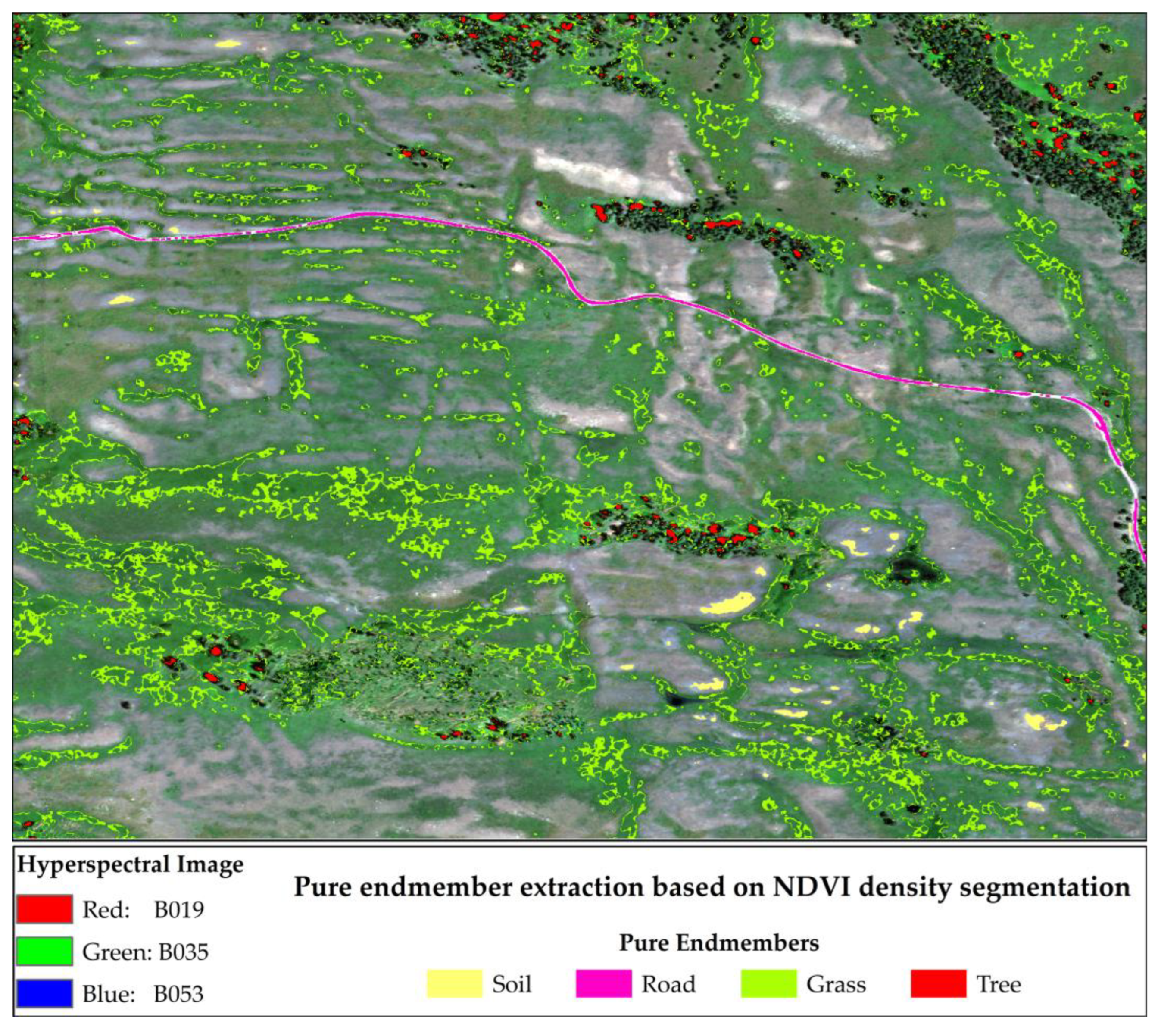
Figure 4.
Spectral characteristics curves of soil, grass, road and trees.
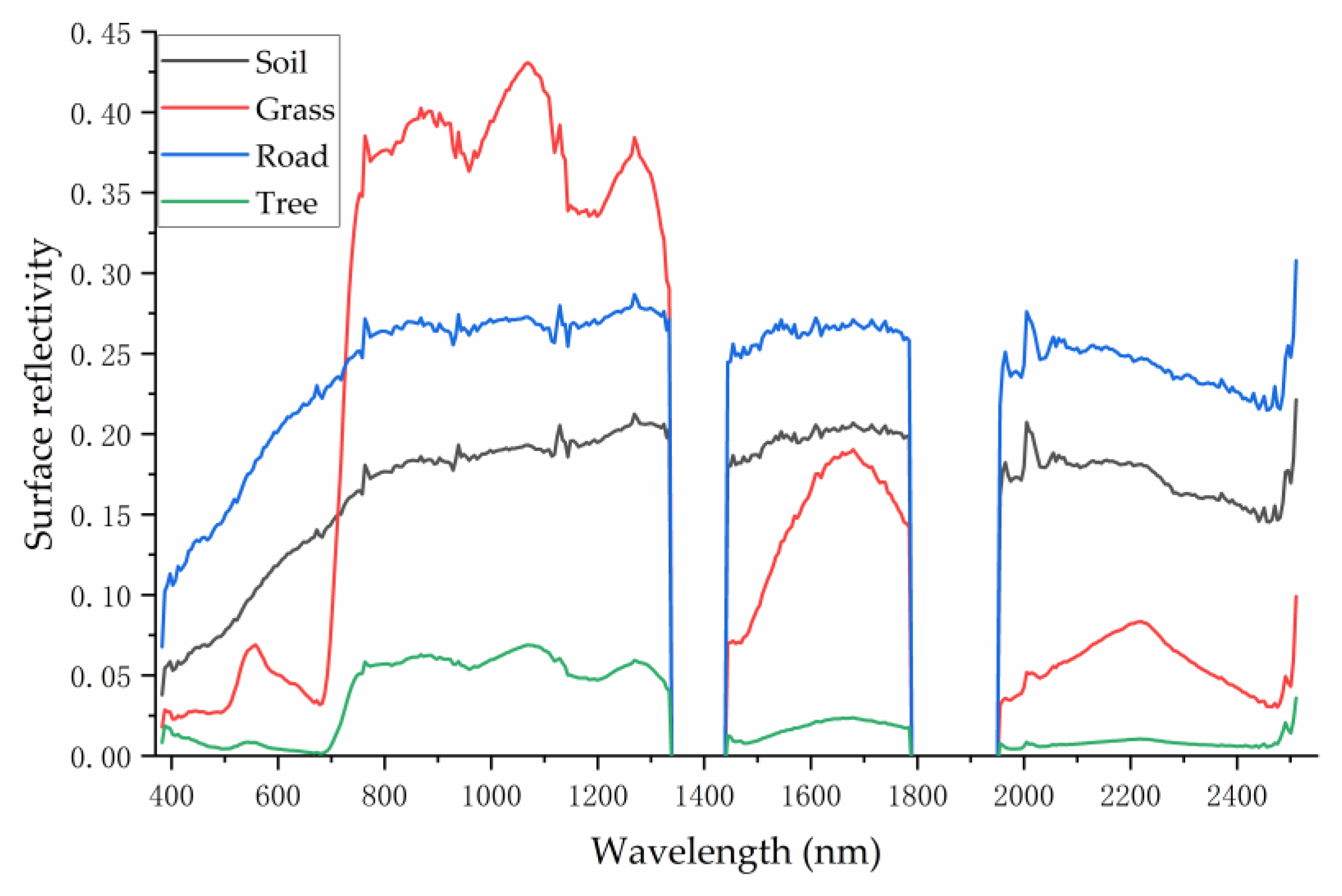
Figure 6.
Probability and cumulative probability distribution of RMSE in endmember abundance estimation for the test area.
Figure 6.
Probability and cumulative probability distribution of RMSE in endmember abundance estimation for the test area.
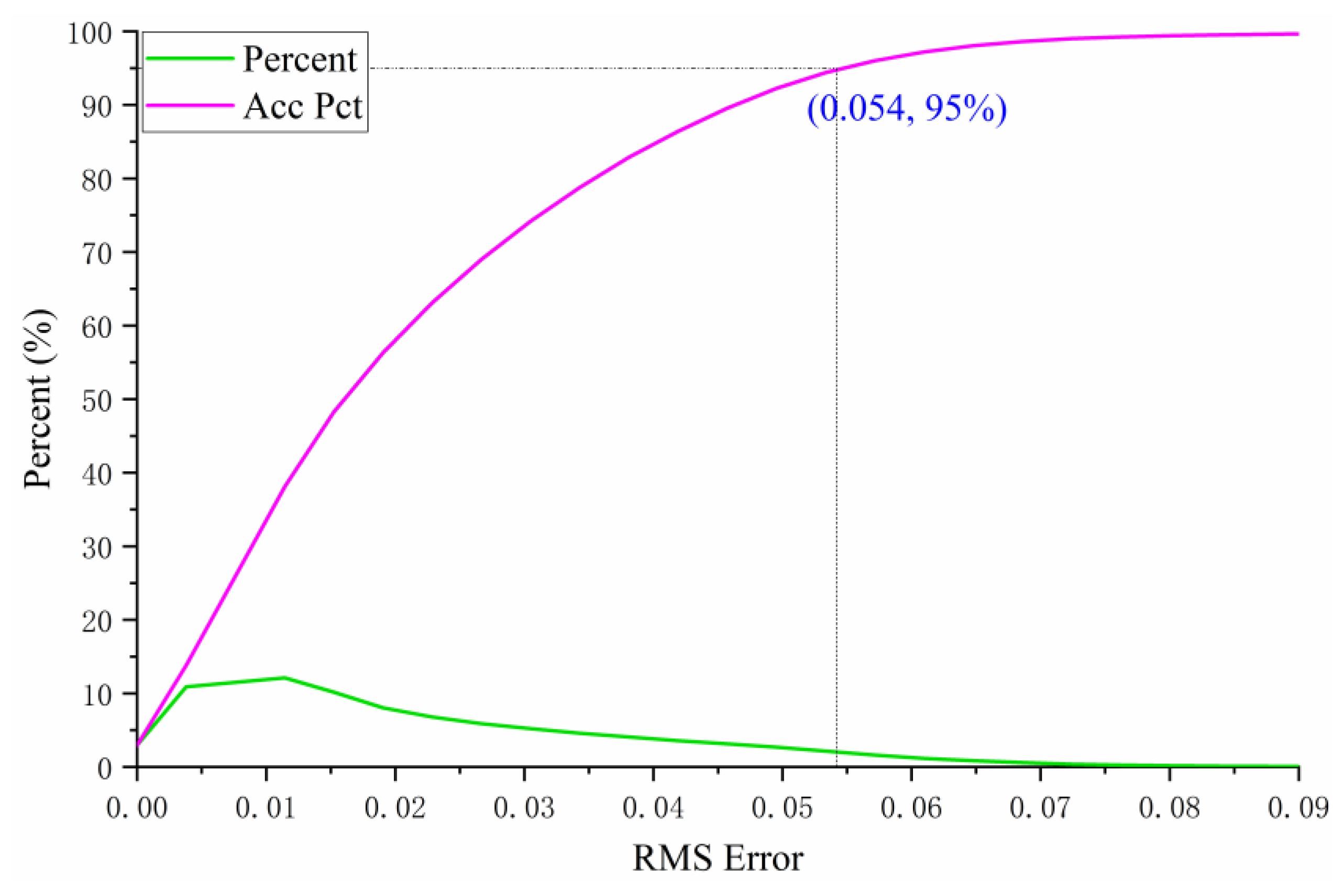
Figure 7.
Estimation results of backscattering coefficients of four endmembers in the test area.
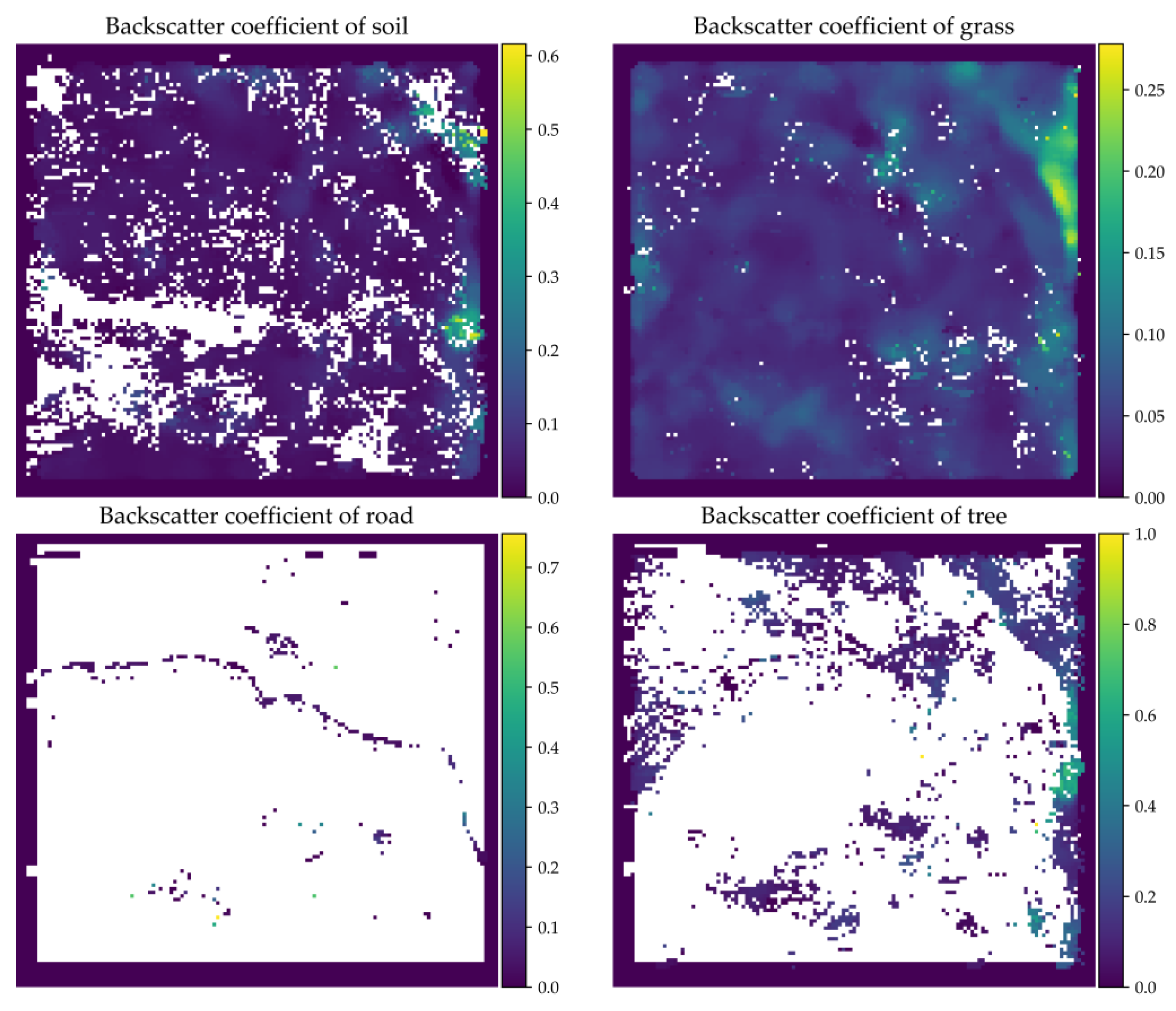
Figure 8.
The proportion and spatial distribution of different types of pixels in the test area.
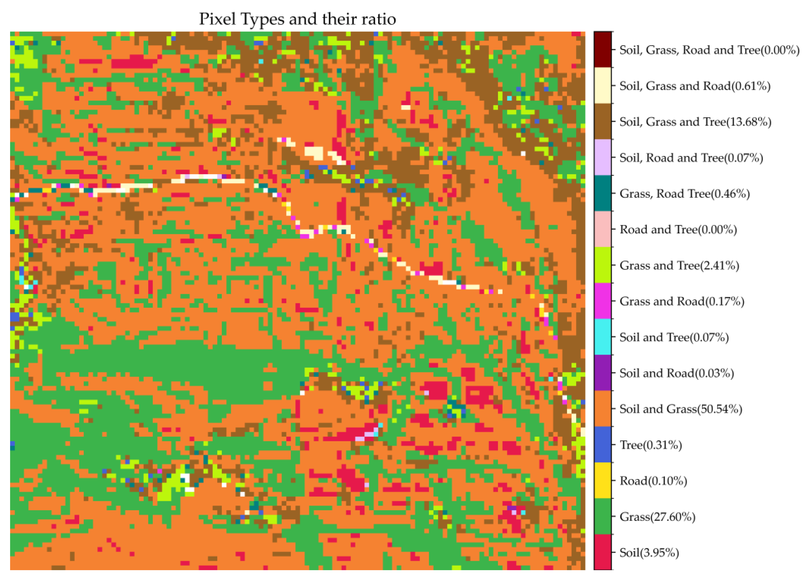
Figure 9.
Relative error of soil and grass backscatter coefficient estimation.


Table 1.
Types, codes and proportions of pixels in the test area.
| Endmembers numbers in pixel | Pixel types | Endmember Coding | Pixels Number | Ratio(%) |
|---|---|---|---|---|
| 1 | Soil | 0 | 577 | 3.95 |
| Grass | 1 | 4037 | 27.60 | |
| Road | 2 | 14 | 0.10 | |
| Tree | 3 | 46 | 0.31 | |
| 2 | Soil and Grass | 4 | 7392 | 50.54 |
| Soil and Road | 5 | 4 | 0.03 | |
| Soil and Tree | 6 | 10 | 0.07 | |
| Grass and Road | 7 | 25 | 0.17 | |
| Grass and Tree | 8 | 353 | 2.41 | |
| Road and Tree | 9 | 0 | 0.00 | |
| 3 | Grass, Road Tree | 10 | 68 | 0.46 |
| Soil, Road and Tree | 11 | 10 | 0.07 | |
| Soil, Grass and Tree | 12 | 2000 | 13.68 | |
| Soil, Grass and Road | 13 | 89 | 0.61 | |
| 4 | Soil, Grass, Road and Tree | 14 | 0 | 0 |
Disclaimer/Publisher’s Note: The statements, opinions and data contained in all publications are solely those of the individual author(s) and contributor(s) and not of MDPI and/or the editor(s). MDPI and/or the editor(s) disclaim responsibility for any injury to people or property resulting from any ideas, methods, instructions or products referred to in the content. |
© 2025 by the authors. Licensee MDPI, Basel, Switzerland. This article is an open access article distributed under the terms and conditions of the Creative Commons Attribution (CC BY) license (http://creativecommons.org/licenses/by/4.0/).
Copyright: This open access article is published under a Creative Commons CC BY 4.0 license, which permit the free download, distribution, and reuse, provided that the author and preprint are cited in any reuse.


