
Submitted:
30 April 2025
Posted:
30 April 2025
You are already at the latest version
Abstract
A machine learning framework is developed to interpret vehicle subsystem status from sensor data, providing actionable insights for adaptive control systems. Using the vehicle’s suspension as a case study, inertial data are collected from driving maneuvers including braking and cornering, to seed a prototype XGBoost classifier. The classifier then pseudo-labels a larger exemplar dataset acquired from street and racetrack sessions, which is used to train an inference model capable of robust generalization across both regular and performance driving. An overlapping sliding-window grading approach with reverse exponential weighting smooths transient fluctuations while preserving responsiveness. The resulting real-time semantic mode predictions accurately describe the vehicle’s current dynamics and can inform a model predictive control system that can adjust suspension parameters and update internal constraints for improved performance, ride comfort, and component longevity. The methodology extends to other components, such as braking systems, offering a scalable path toward fully self-optimizing vehicle control in both conventional and autonomous platforms.
Keywords:
automotive
; data-driven
; dynamics
; informatics
; machine learning
; model predictive control
1. Introduction
Machine Learning (ML) is revolutionizing the way vehicles perceive and interact with their environment [1]. In this context, ML techniques are used to process and interpret vast amounts of sensor data from various sensors to recognize patterns and predict critical variables such as object locations, road conditions, and driver behavior. ML excels at handling the complex, nonlinear, and uncertain dynamics that traditional physics-based models may not fully capture [2]. For example, ML algorithms can classify road surfaces, detect obstacles in real time, and even forecast potential hazards before they occur. This data-driven approach provides vehicles with enhanced situational awareness and decision-making capabilities, enabling them to adapt to changing driving scenarios [2]. In essence, ML transforms raw sensor inputs into actionable insights, laying the foundation for smarter, safer, and more efficient vehicle control systems.
Model Predictive Control (MPC) is widely researched and implemented in the realm of vehicles and advanced driver assistance systems [1]. MPC predicts the future state of a system by using a mathematical model subject to constraints [3]. In automotive applications, this can mean forecasting the vehicle’s future position based on its current speed and dynamics. For instance, in trajectory control, a vehicle is required to track a desired path over a curved section of road. A simplified kinematic or dynamic model describes the vehicle’s motion while constraints such as maximum steering angle and acceleration are enforced [3]. The vehicle’s sensors (e.g., cameras and LiDAR) provide real-time estimates of its state which include position, velocity, and heading. At each control step, MPC formulates an optimization problem by minimizing a cost function subject to these constraints, computes the optimal sequence of control actions over a prediction horizon, and executes the appropriate actions [2]. This process repeats continuously, enabling robust control.
MPC works well in environments where system dynamics are well understood and remain relatively constant, while ML excels at analyzing data and adapting. While these systems can function independently for many tasks, a hybrid system model that leverages the strengths of both can be explored.
1.1. Applications
1.1.1. Brakes
The practical applications and implementation of this hybrid model can be demonstrated by examining its impact on various vehicle systems and components. When the brakes in a vehicle are used, kinetic energy is converted into heat energy. This heat causes the coefficient of friction between the rotor and brake pad to decrease. Consequently, the brakes may be less effective during subsequent uses, increasing stopping distances. To address this issue, a machine learning model can be trained with data such as temperature and recorded stopping distances. This model would be used to grade new data and output a health score reflecting the current braking capability. This information would then be used to adjust the MPC model. In practical terms, this means that the MPC can preemptively adjust its control strategy, to for instance, initiate earlier braking to compensate for the increased stopping distance. Moreover, this approach is not limited to one-way communication. The MPC can also provide feedback to the ML model, helping to refine its predictions, and as in this example, evaluate whether early braking was indeed necessary. By having the MPC aware of the current brake power available, its constraints can be adjusted rather than using a fixed set of parameters that may not accurately reflect current conditions. Several benefits are to be had: increased safety by reducing the risk of collisions due to insufficient braking; improved ride quality for passenger carrying vehicles by avoiding abrupt or jarring decelerations; extended component life for brake rotors, pads, and related parts through better overall control, especially for commercial vehicles bearing large loads; and faster lap times around a track by alerting the user of brake status.
1.1.2. Assistance
Traction and stability control are among the most critical functions for a vehicle. Dynamically changing factors such as tire temperature, age, tread condition, air pressure, as well as external variables like uneven or wet roads and hazards such as rocks, drastically impact available traction. A machine learning model can be trained on historical data from these scenarios to predict available traction based on real-time sensor readings, such as humidity. In a hybrid ML–MPC system, the outputs of the ML model are used to dynamically update both the constraints and the weighting factors in the MPC’s cost function. For example, if the ML model indicates reduced available traction due to adverse conditions, the MPC can lower the maximum allowable tire slip and impose higher penalties on aggressive control actions, such as rapid throttle inputs or abrupt steering. This dual adaptation mechanism ensures that the control system remains tuned to current driving conditions, ultimately enhancing both vehicle performance and safety.
1.1.3. Suspension
Most modern cars feature an electronically adjustable suspension. By analyzing data from sensors such as accelerometers, ML can determine when to stiffen the suspension for improved handling. Conversely, if the ML model outputs a score indicative of poor road conditions, the suspension can be loosened for increased compliance. This concept can extend to high-end suspension setups, such as multi-way adjustable coilovers. Currently, these components require manual adjustments by turning a knob underneath the car, limiting the vehicle to a single configuration at any given time. A performance-oriented set of 3-way adjustable coilovers by German automotive brand KW Suspensions offers 16 different settings for rebound dampening, 6 clicks for low-speed compression, and 14 for high-speed compression, resulting in 1,344 possible combinations [4]. Their 4-way adjustable coilovers allow for 13 adjustments for each low and high-speed compression and rebound, resulting in 28,561 combinations. Tuning such a setup is labor-intensive, and there is no one-size-fits-all configuration, as road conditions can vary dramatically. If these parameters could be adjusted in real time using a hybrid ML–MPC system where MPC continuously optimizes control based on ML predictions, the vehicle could achieve unprecedented levels of comfort and performance while improving wear on bushings, springs, tires, and requiring less maintenance rebuilds on dampers.
1.1.4. Race Vehicles
Another compelling use case is in designing high-performance autonomous vehicles for racetrack applications [5]. While such vehicles can be preprogrammed to drive optimally for a specific track, a vehicle employing the hybrid ML–MPC model can dynamically adapt to any road course without the need for track-specific tuning. In essence, the hybrid model equips an autonomous vehicle with driver-like intuition. Whereas a skilled human driver relies on feel, an autonomous vehicle outfitted with ML and MPC can process and take into consideration vast amounts of both historical and real-time data to adjust to any condition. Such a tool offers significant benefits for product development. For instance, manufacturers of tires, brakes, and aerodynamic parts, could push their products to the limit, gathering objective testing data that drives further improvements. Additionally, the system enhances safety by allowing extreme-condition tests, regardless of their nature, to be conducted autonomously, thereby eliminating risk to human drivers. Ultimately, the autonomous vehicle serves as a benchmark, offering insights into the boundaries of performance and giving drivers a clear understanding of what is possible before they attempt similar maneuvers themselves.
1.2. Hybrid Framework
The benefits of a hybrid approach can also be assessed through the weaknesses of each model and how the integration mitigates them. First, consider how the hybrid approach addresses ML’s drawbacks. MPC relies on explicit mathematical models, clearly defined constraints, and a cost function that quantifies its objectives. Each action is derived through an optimization process in which every element of the formula is known [3]. In a sense, MPC in the hybrid approach translates ML outputs into actionable commands in the real world. This transformation mitigates ML’s inherent black box nature by providing a means to interpret and validate its methods and outputs. If ML generates an output that is unreliable, its manifestation in the physical world is still subject to MPC’s jurisdiction. Picture that one of the sensors the ML model uses to grade brake performance malfunctions, resulting in noisy data, outliers, or no data at all due to an overheated sensor, loose connection, or some electronic logic failure. The output of the ML component in this case can be nonsensical, and if the vehicle were to rely on it without contestation or verification, it could cause an undefined state. MPC, through its rule-based framework, can override or correct such ambiguous outputs, ensuring indeterminate vehicle actions are not executed.
Next, the hybrid model’s mechanisms for overcoming MPC’s limitations are examined. MPC operates in a receding horizon manner, optimizing the control strategy over a finite future window while implementing only the first control action [3]. This approach, however, assumes that each action moves the system into a state where subsequent adjustments can be made effectively. If an action causes the system to deviate too far from the desired state, such as from unexpectedly low deceleration, it may force the system into a condition where only drastic recovery measures can restore stability, ultimately leading to unsafe maneuvers and conditions [3]. In a circumstance where the brakes have completely failed, the vehicle can even exceed beyond its state of recovery, necessitating extreme corrective measures that fall outside physical constraints and possibilities. ML’s anomaly detection, information handling, and prediction can mitigate this scenario by alerting MPC of brake failure before any braking action is initiated.
In both cases, the system can trigger a fail-safe mode designed to handle abnormal conditions, rather than merely relying on the system to self-correct, which can lead to catastrophic events. The hybrid model uses MPC’s transparency to reveal ML’s opaqueness, while it uses ML’s foresight to offset MPC’s heavy reliance on feedback.
1.3. Machine Learning Module
To implement a hybrid system, the ML and MPC models must be developed. ML models can be trained on sensor log data to assess vehicle parameters [6]. This paper focuses on demonstrating the ML component of a potential hybrid system. The process of designing a ML model that can be used to inform control systems in the vehicle is shown in Figure 1.
2. Materials
2.1. Focus
The objective is to develop a machine learning model that ingests real-time vehicle sensor data, interprets system states, and generates predictive insights to inform control strategies. While any vehicle subsystem can be used if data can be collected from it, vehicle dynamics is chosen as the representative example in this paper. Inertial data grading can be used for suspension control, among other applications such as Drag Reduction Systems (DRS). Vehicle dynamics data are obtained from an inertial measurement unit (IMU), which combines tri-axial accelerometer and gyroscope readings.
2.2. Equipment
The vehicle used is a BMW production vehicle fitted with its original factory suspension setup and 300-treadwear tires. The collected data were acquired using a RaceBox Mini performance meter, an automotive telemetry device capable of timing quarter-mile runs and track laps via a 25 Hz GPS module (10 cm accuracy). RaceBox Mini also features a 1kHz sampling-rate accelerometer with ±8G scale with 0.001G sensitivity, and a 1kHz sampling rate gyroscope with ±320dps scale with 0.02dps sensitivity [7]. The device is controlled via the RaceBox mobile application. After each session, data are automatically uploaded to the user’s account and made available for download as CSV files. Although the accelerometer and gyroscope sample internally at 1 kHz, recorded data follow the GPS’s 25 Hz sample rate, yielding 25 rows per second (0.04s per row).
The RaceBox is positioned in the center armrest of the vehicle, providing a central location both horizontally and vertically. It is secured using double-sided tape and Velcro, and is placed flat. While GPS accuracy and location data are not of primary interest, it is important that the RaceBox maintains a sufficiently strong GPS signal to consistently achieve its maximum data rate of 25 Hz. Signal strength depends on the number of satellites in view and the quality of the signal, which can be influenced by obstructions between the device and the satellites. The armrest is constructed of hard plastic with an Alcantara covering, and directly above is a glass moonroof with a fabric liner. Even under cloudy conditions, the RaceBox in this position achieved a reliable GPS signal.
2.3. Procedure
To begin data collection, the user connects to the RaceBox using the mobile application. The automated Z-axis calibration is performed first, which zeroes the sensor readings based on the device’s current orientation. Following this, an X-axis calibration is completed by accelerating the vehicle forward for a few seconds. Logging is initiated by selecting “New Track Session” and then “Drive Without a Track,” placing the device into continuous recording mode. The session can be ended at any time by selecting the back arrow.
It should be noted that this study prioritizes performance-oriented suspension tuning over ride-comfort considerations. To more accurately assess adverse road conditions, it would be more appropriate to mount four IMUs and vibration sensors on unsprung components, such as the wheels, since the suspension attenuates many of these forces before they reach a single cabin-mounted IMU. Consequently, the data logging instrument may prove insensitive to bad roads unless the vehicle is equipped with a stiff race suspension.
2.4. Code
All programming tasks were performed using Python 3.12.5 within a Jupyter notebook environment.
3. Data Collection
3.1. Features
The data to be collected are six-dimensional: three features from the accelerometer and three from the gyroscope.
3.1.1. GForceX
Defined as longitudinal acceleration, this feature measures the forward and backward acceleration of the vehicle. A positive value corresponds to acceleration (throttle) while a negative value corresponds to deceleration (braking).
3.1.2. GForceY
Known as lateral acceleration, this feature measures side-to-side acceleration. Positive values correspond to the vehicle and steering wheel turning left (or traveling counterclockwise in a roundabout), while negative values correspond to the vehicle and steering wheel turning right (or traveling clockwise in a roundabout). This feature captures the bulk of weight transfer during cornering.
3.1.3. GForceZ
Known as vertical acceleration, this feature measures the upward and downward acceleration, which can be caused by uneven roads, bumps, or potholes. The reading is 1.0 when the vehicle is stationary on level ground. Deviations above 1.0 indicate upward, while deviations below 1.0 indicate downward movement.
3.1.4. GyroX
Known as roll rate, this feature measures the angular velocity along the longitudinal axis. A positive value indicates clockwise rotation, while a negative value indicates counterclockwise rotation. As the vehicle is constrained to the road, this value detects chassis lean. Larger magnitudes indicate faster changes in the body roll.
3.1.5. GyroY
Known as pitch rate, this feature measures the angular velocity about the lateral axis. Using the front of the vehicle as an example reference point, a positive pitch corresponds to the front lowering, while a negative pitch corresponds to the front rising. This behavior can occur during braking (nose dive), during acceleration (rear squat), or during sharp transitions over uneven roads.
3.1.6. GyroZ
Known as yaw rate, this feature measures the angular velocity about the vertical axis. Yaw rates correlate with steering-induced direction changes, where a positive yaw rate indicates counterclockwise rotation and a negative yaw rate indicates clockwise rotation. Situations such as understeer, where the front tires lose grip before the rear and push the vehicle wide, result in smaller-than-expected values, while oversteer, where the rear tires lose grip before the front and spin the tail outward, result in higher-than-anticipated values.
3.1.7. Sensor Metrics
It is important to note that these values include the gravity component. As a result, the accelerometer readings when the device is at rest are 0.00 gx, 0.00 gy, and 1.00 gz. When the device is moved, these values change and remain offset unless the device returns to its original orientation. This means that the three-axis orientation of the device influences acceleration values even when the device is at rest. Although it may seem that the gravity component confounds dynamic accelerations, it should not be removed, as gravity is a real force acting on the vehicle. For example, the GForceX value during braking on a downhill will register a greater negative value compared to braking on level ground, all else being equal. Removing the gravity component would result in a model that does not accurately represent real-world forces, as in this case, there is more load on the suspension when braking downhill than on flat ground. This extends to other scenarios as well, including GForceY during cornering on inclined or declined surfaces. The gyroscope values, in contrast, change only when there is a change in rotational position, with the magnitude indicating how quickly that rotation is occurring.
The analysis provided in Section 3.1 only covers basic dynamics and considers each sensor value individually. While it may be possible to theoretically model the interactions between the features to some extent, machine learning inherently captures all relationships and patterns across any scenario, providing a more complete and representative picture.
3.2. Seed Collection
The seed collection stage, shown in Figure 1, serves as the foundational dataset for training the initial classifier. It consists of well-defined and manually curated examples that represent distinct scenarios. These labeled samples are critical for establishing baseline patterns, which will later be used to expand the dataset through pseudo-labeling.
The type of data recorded depends on the driving maneuver. The seed collection was compiled using three separate sessions for each of four scenarios: braking, launching, low speed cornering, and high speed cornering, and a single longer session for normal driving.
3.2.1. Normal
This data consists of cruising at a fairly constant speed of 42.5 mph on a relatively flat road.
3.2.2. Launch
- Session 1: Rolling launch to 90 mph.
- Session 2: Hard launch from a complete stop to 97 mph.
- Session 3: Hard launch using brake boosting (for maximum torque), from a complete stop to 55 mph.
3.2.3. Brake
- Session 1: Hard braking from 47 mph to a complete stop.
- Session 2: Hard braking from 71.5 mph to 34 mph.
- Session 3: Soft to moderate braking from 49.5 mph to a complete stop. Naturally, this session contains more data than Session 1 and Session 2, as it took longer to stop.
3.2.4. Low Speed Corner
- Session 1: A roundabout with relatively flat elevation.
- Session 2: A roundabout featuring varying inclines and declines.
- Session 3: A dual-lane roundabout, as opposed to a single-lane, resulting in a larger outer radius.
3.2.5. High Speed Curve
- Session 1: A curved section taken at 88 mph.
- Session 2: A curved section taken at 94 mph.
- Session 3: A curved section taken at 98 mph.
3.3. Exemplar Data Set
The exemplar data set represents a much larger and more realistic collection of driving conditions compared to the seed collection. While the seed collection consists of carefully isolated and manually verified maneuvers, the exemplar data set captures continuous, natural driving that includes a mixture of all scenarios—braking, launching, low-speed cornering, high-speed cornering, and normal driving. The exemplar data set consists of two sources: Street and Track driving data.
3.3.1. Street
This data was collected from regular to spirited street driving. It includes accelerations, decelerations, low and high-speed curves, straights, and roads of varying shapes and sizes.
3.3.2. Track
This data was collected from a session at the Las Vegas Motor Speedway – Outside Road Course, a roughly 2.4-mile short circuit featuring 13 turns, along with straights and low and high-speed sections. The session included the entry lap, five complete laps, and the exit lap. The driving style was as aggressive as possible to push the car to its limit and achieve the fastest lap times.
3.4. Processing
Figure 2 shows an example CSV file after downloaded from the user’s Racebox account.
Each file contains 13 columns, but the features of interest are: GForceX, GForceY, GForceZ, GyroX, GyroY, and GyroZ. The data that constitute the seed collection should be of high quality, as they serve as the representative examples for each specific maneuver. Since logging is started before the maneuver is executed and stopped afterward, rows outside the maneuver of interest must be removed. The speed column, along with the six feature columns, is useful for identifying when a maneuver begins and ends. Additionally, the RaceBox website provides an overlay of the data points on a satellite map, which helps visually confirm entry and exit points for maneuvers such as roundabouts.
After isolating the rows corresponding to the maneuver, the remaining irrelevant rows are deleted. Next, any column that is not one of the six selected features is removed. Finally, a new column corresponding to the scenario label is introduced. A numerical value is assigned to represent the type of maneuver according to the following legend:
- Normal: 1
- Launch: 2
- Brake: 3
- Low Speed Corner: 4
- High Speed Curve: 5
All rows in the seed collection files are assigned the appropriate label. There are 13 files in total. These files are combined into a single CSV file that represents the training data from the seed collection. A portion of it is shown in Figure 3.
The two files that make up the exemplar data set are also processed. For these files, rows before and after the driving sessions are retained, as they are considered part of the overall driving behavior and no manual trimming is performed. The unnecessary columns are removed, leaving only the features of interest. The two files are then combined into a larger file. Due to the sheer size and unorganized nature of the exemplar data set, labeling is not feasible at this stage.
4. Machine Learning Framework
4.1. Prototype Classifier
The first step is to run a classifier on the training data derived from the seed collection process. The model is trained to capture sensor patterns and associate them with specific maneuvers. This model, referred to as the prototype classifier, will be used to label the exemplar data set. XGBoost [8] proved most effective and was selected to construct the prototype classifier, with other machine learning algorithms such as Random Trees also being evaluated [6]. The training data were split into an 80/20 ratio for training and testing. Stratification was used, as the dataset contains varying numbers of rows for each label, helping prevent the model from becoming biased toward the majority class. A 5-fold cross-validation grid search was performed for hyperparameter tuning. The best parameters found were:
- Learning rate: 0.2
- Max depth: 3
- Estimators: 200
The model achieved a test accuracy of 98.9% by using the trained model to classify the withheld test data and comparing the predicted labels to the true labels.
4.2. Pseudo-Labeling
The second step is to use the newly trained prototype classifier to label the exemplar data set. The exemplar data set, consisting of the processed but unlabeled data from the street and track driving, is loaded, and each row’s label is predicted using the prototype classifier. This process results in the exemplar data set now containing a label column for each row. By using semi-supervised learning, groupings are constrained to the target modes and avoid the ambiguous, hard-to-verify clusters produced by purely unsupervised methods, while automating a labeling process that would be impractical under a fully supervised approach.
4.3. Inference Model
The third step is to train a model using the exemplar data set. XGBoost is again used for this task, with the max depth parameter set to 5. The model achieved a test accuracy of 97.6%. A small drop in accuracy compared to the prototype classifier trained on the seed collection is observed. This is expected, as the seed collection was manually curated and verified to be as accurate as possible. In contrast, the exemplar data set was pseudo-labeled, meaning its labels were assigned automatically by a model that, while highly accurate, was not perfectly accurate, introducing an inherent compounding loss. Another potential contributing factor to the decrease in accuracy is the increased noise present in the exemplar data set, as it is derived from a broad heterogeneity of sensor values. Despite the slight loss in accuracy, it is important to emphasize that the exemplar data set by nature is better at generalizing to real-world driving data than the prototype classifier, satisfying one of the primary objectives.
Figure 4 presents XGBoost’s F-score metric, known as feature importance, which tallies how often each feature is selected to split a node during tree construction [8]. The ranking provides insight into how useful each feature is when partitioning the data. Analysis of the plot shows that longitudinal forces, lateral forces, and yaw rate are the most important signals. They are followed by pitch rate and roll rate. The least informative feature is vertical acceleration. Note that these scores are influenced by the specific training data, and different datasets or objectives could reorder the feature scores.
4.3.1. Sliding Window
The inference model is intended to operate in real-time, and as such, a sliding window approach is used. The window advances every 40 milliseconds, matching the 25 Hz sample rate. Each window holds and processes 50 rows of data, corresponding to 2 seconds’ worth of information. This means that the first prediction occurs at the 2-second mark. At this moment, the window begins operating in a FIFO-like (First-In-First-Out) manner. As the window advances by another 0.04-second step, the oldest row of data is removed, and the newest row is added to the head of the window. Predictions are programmed to be generated every 1 second, corresponding to 25 new rows of data. An overlapping sliding window is implemented to smooth transitions between predictions. Half of the window consists of the previous second of data, and the other half contains the current second. This overlap dampens the output, as each prediction is based on both historical and current data. As a result, sequential predictions are more likely to be similar rather than different. This behavior prevents abrupt changes in classification outputs unless a warranted driving transition occurs, reducing the risk of oscillations that could destabilize the vehicle if acted upon.
4.3.2. Weighting
Given the need to maintain responsiveness to current conditions, reverse exponential weighting is applied. This approach emphasizes the most recent measurements while still retaining information from earlier samples. The weights are computed as:
where is the raw (unnormalized) weight assigned to the sample, i is the position of the sample within the window (with being the oldest and being the newest), and N is the window size, which in this case is 50. The oldest sample, receives a weight of , and the newest sample receives a weight of . When aggregating the per-row class-probability vectors within the window, each vector is multiplied by its corresponding weight , and the results are normalized via a weighted average.
Since the application is performance-focused, an exponential weighting curve is used. If a less aggressive response were desired, a different strategy, such as a linear ramp, could be employed instead. This weighting scheme, combined with the sliding window, enables the classifier to respond quickly to changes in driving conditions while preserving sufficient historical context to prevent transient, single-sample fluctuations from dominating the overall scenario estimate.
4.3.3. Grading
When a new row arrives into the window, its feature vector is fed into the inference model. This results in a probability distribution vector over the classes:
where i indexes the sample and k indexes the class. The six-dimensional sensor data are input into the XGBoost model, and a probability distribution vector across five classes () is produced.
Next, the per-sample probability vectors are combined to form a single window-level prediction. First, each probability vector is multiplied by its corresponding weight :
The model’s weighted beliefs are then aggregated across the window:
The normalization factor is calculated:
Computing Equation (6) yields the smoothed, window-level probability vector. The class corresponding to the largest element in is selected as the prediction for the window. For example, if the third element is the largest, the index is mapped to the corresponding scenario, , meaning the windowed sensor data most closely matched a braking maneuver.
This method proved to produce more robust predictions compared to simpler schemes, such as majority voting, where the hard label at each sample is taken and the most frequent label is selected.
5. Results
To evaluate performance, a separate track session log was applied as operational test data. This particular track session included a warm-up lap, during which cars are not permitted to pass one another, and a cool-down lap, where braking is minimized and overall pace is reduced to allow cooling of the engine, turbocharger, brakes, and other components. Additionally, the session was conducted with an instructor and was not driven at full pace. The recorded data provide a good balance between track driving and performance street driving, particularly for evaluating suspension behavior.
The Racebox website plots various recorded values with respect to time, and by dragging the cursor along the x-axis, the displayed values update in 0.04-second increments, as shown in Figure 5.
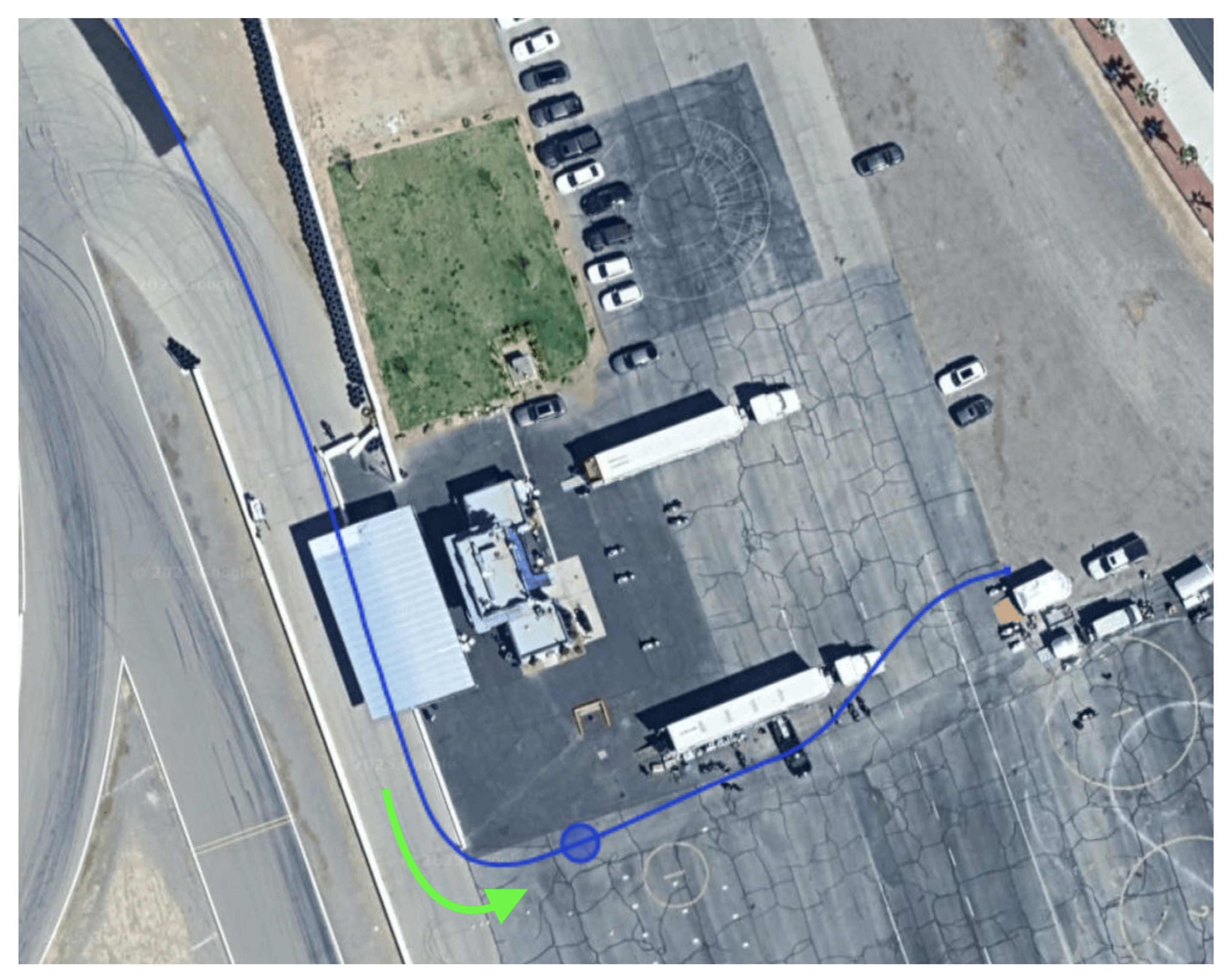
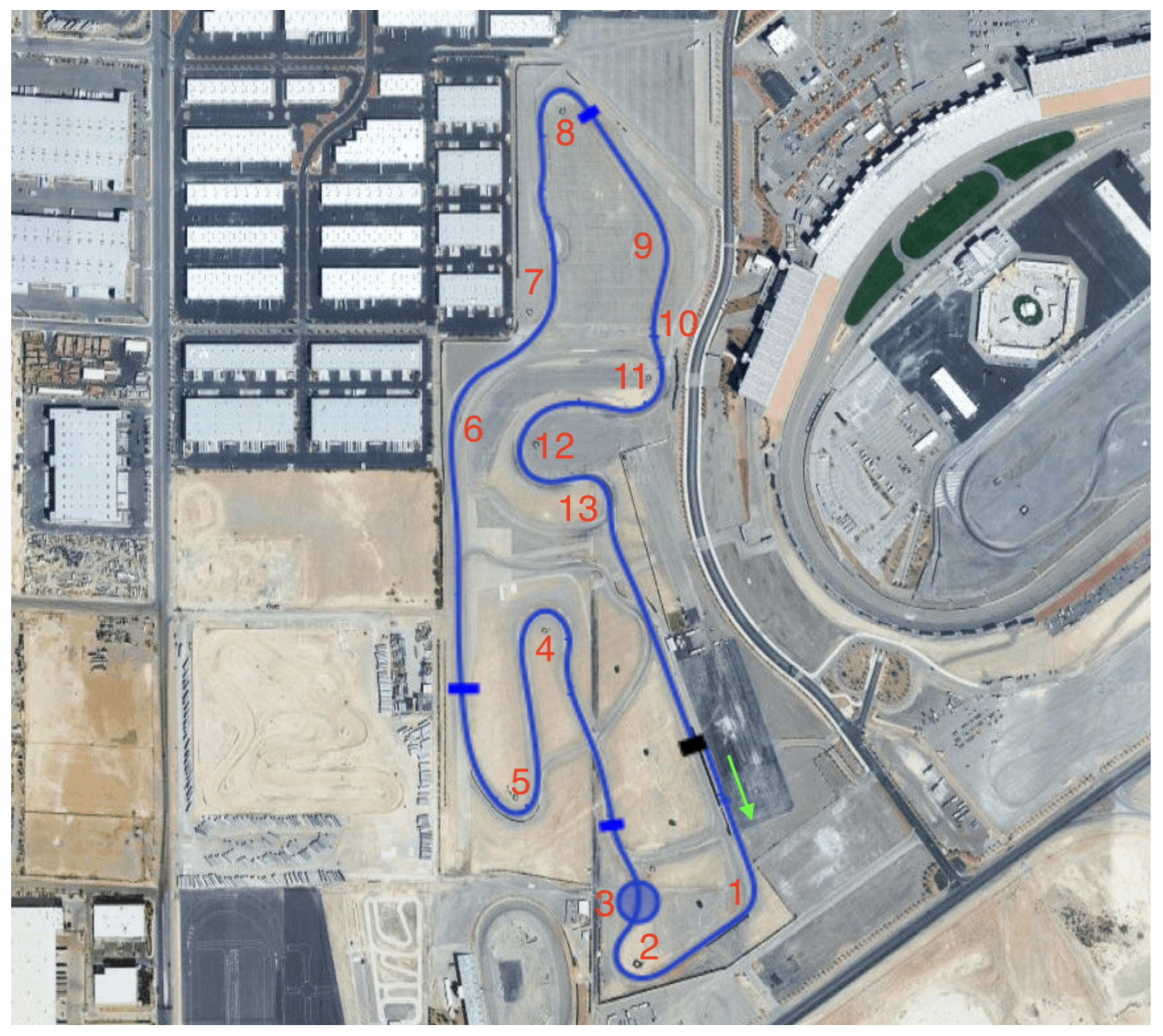
Since Racebox also records GPS coordinates, the position of the vehicle is automatically overlaid onto a satellite map in the online user interface, and the complete path taken by the vehicle during the session can be visualized, as shown in Figure 6.
5.1. Pit Lane
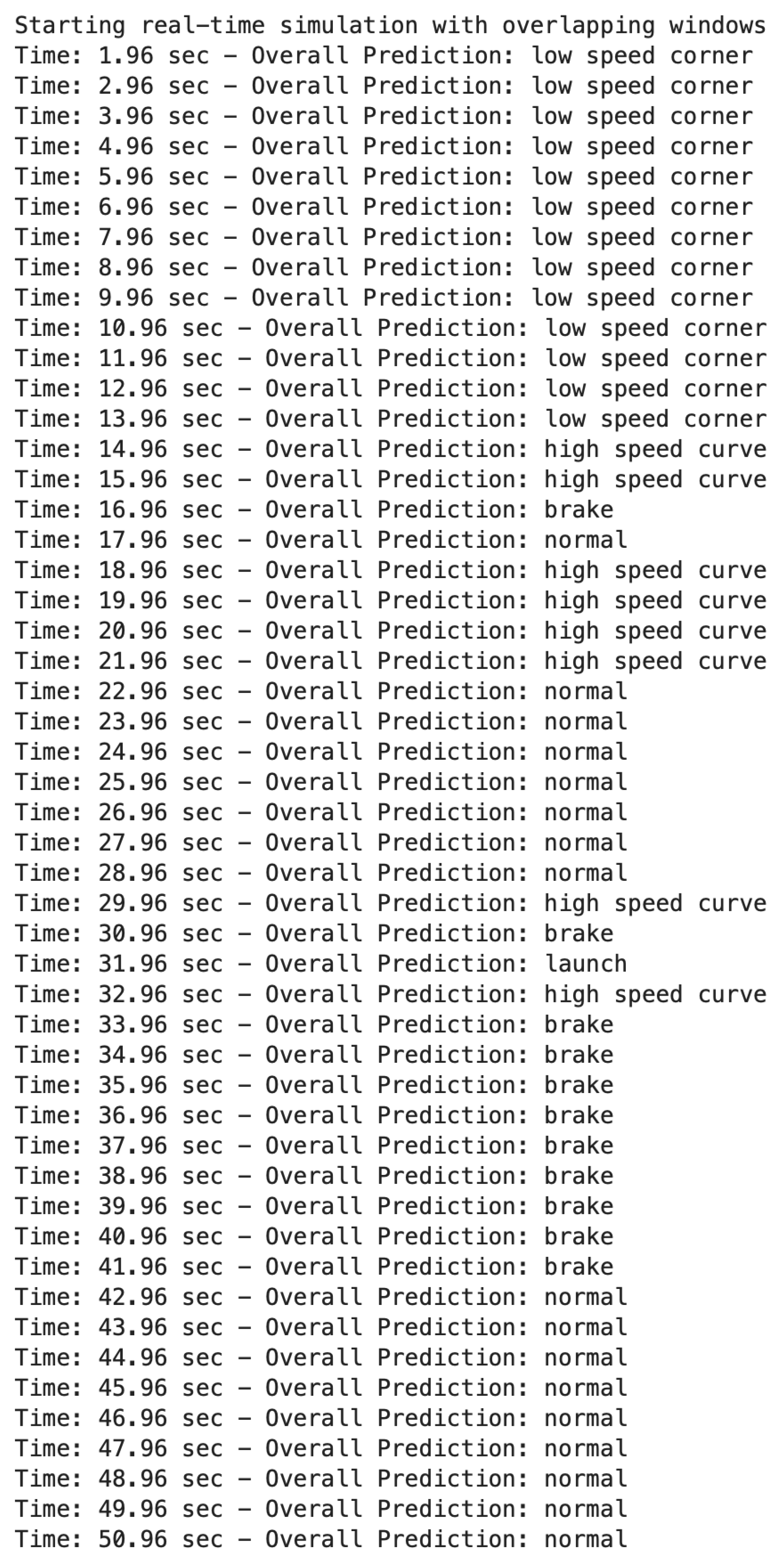
By utilizing the plot and overlay, it is straightforward to verify the model’s output against ground truth. Beginning from the start of the session, the driver is parked and is given a signal to enter pit lane and await entry onto the track. The model outputs are shown in Figure A1, and the corresponding track section is shown in Figure A6. The first 14 seconds of outputs are classified as low-speed corners, which matches the observed road layout. At 15 seconds, there are two outputs classified as high-speed curve, and the RaceBox data show that some acceleration occurred. This suggests that the model associated the sensor values arising from exiting a corner and accelerating to a high-speed curve section. At first glance, it might be expected that this type of scenario could correspond to a launch; however, the vehicle’s suspension is still experiencing weight transfer along the y-axis while exiting the corner. The next two seconds of data are graded as brake and normal. During this period, the acceleration is initially negative, indicating braking, and then returns to zero. The following four seconds are labeled as high-speed curves. Examining the RaceBox data reveals that this section is a straight with minimal acceleration. This shows that the model predictions are aggressive, preferring to label mildly dynamic sections as more aggressive maneuvers rather than as normal driving. This behavior is preferable for track use, where the objective is maximum performance sensitivity; however, for off-track driving, a different calibration or profile could be employed. This tendency is further confirmed by the next seven seconds of outputs, all of which are labeled as normal. This demonstrates that the model can still classify normal driving but requires that the accelerometer and gyroscope values remain relatively tight within the narrow range associated with the normal driving class. The next 20 seconds are split between brake and normal. During this time frame, the driver came to a stop and waited for the track officer’s signal to enter the course.
5.2. Turn 1 - Turn 3
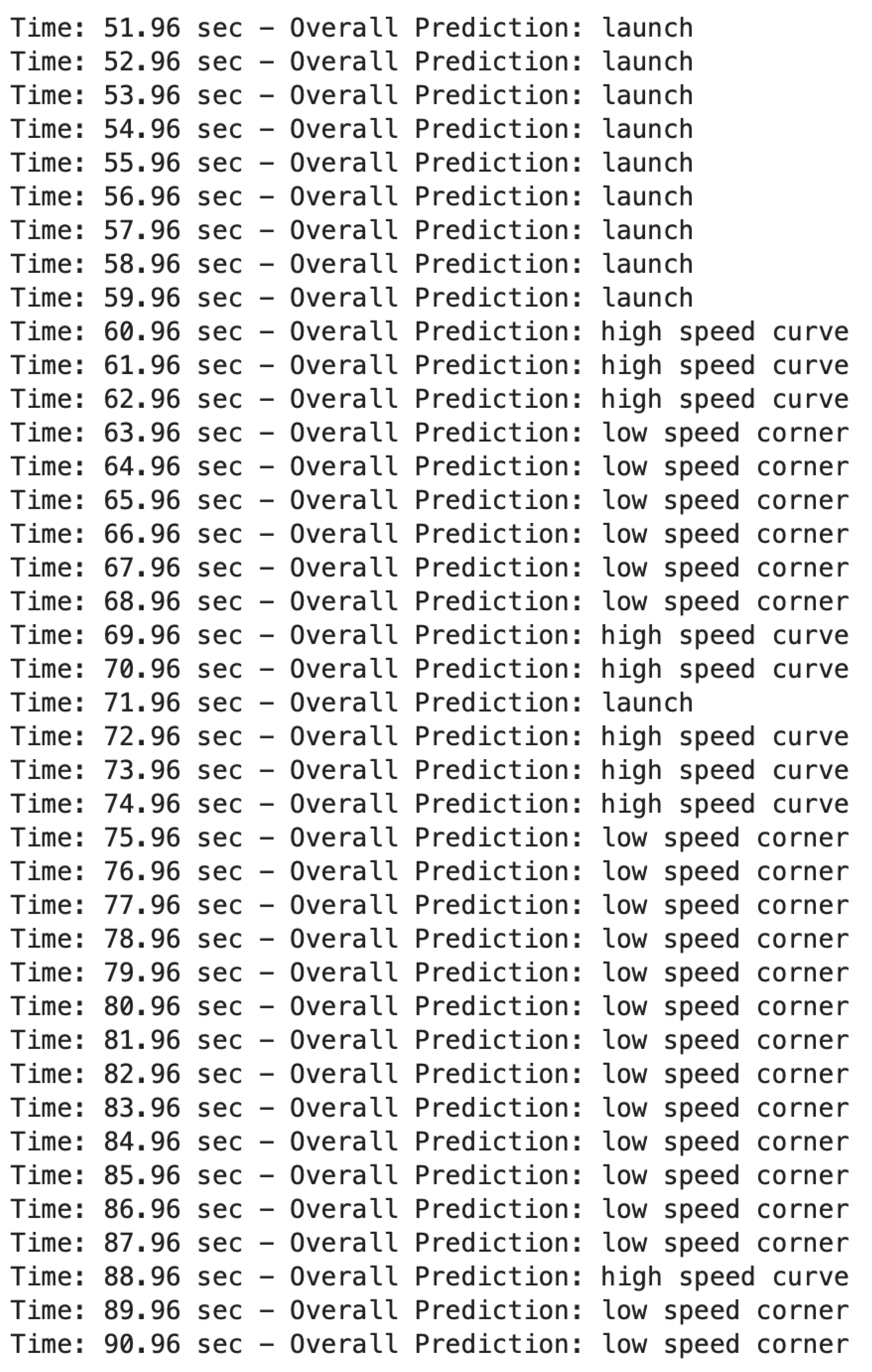
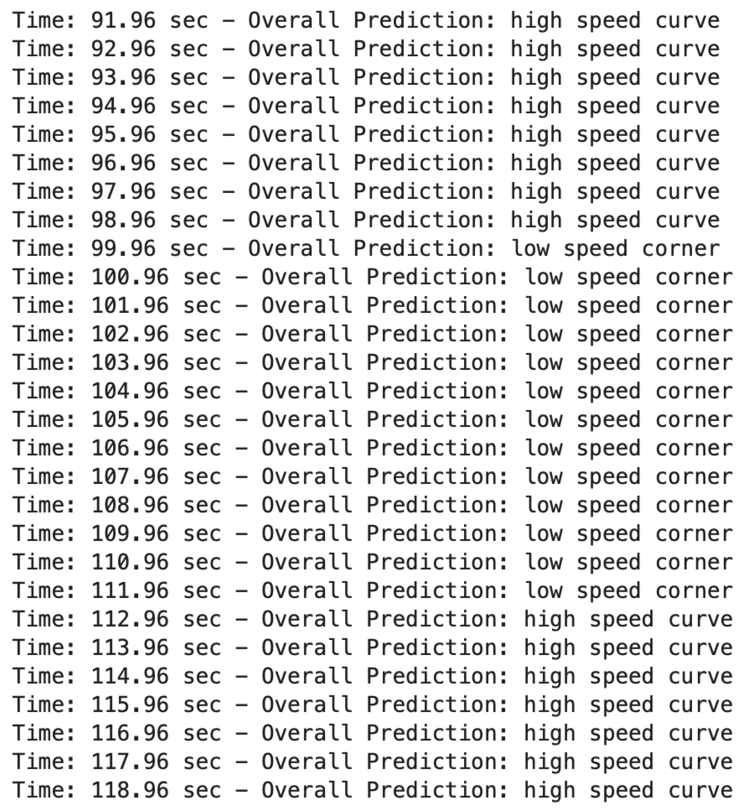
When the driver is given the go signal at 52 seconds, the vehicle launches onto the track. The corresponding outputs can be seen in Figure A2, and the associated track section in Figure A7. As the vehicle approaches the first turn, which is nearly 90 degrees, the model outputs a grade of high-speed curve for three seconds. It may be expected that the driver would brake before such a sharp turn, but the speed was low enough that braking was not necessary. This is due to the fact that the track entry zone is located very close to Turn 1. The model then outputs a label of low-speed corner for a few seconds while the vehicle is in the turn, followed by two seconds of high-speed curve, one second of launch, and three additional seconds of high-speed curve. These outputs correspond to the vehicle straightening out, accelerating, and then entering Turn 2. At this point, the output switches back to low-speed corner. However, it remains on low-speed corner for an extended period. This behavior occurs because the vehicle exits right-hand Turn 2 and immediately transitions into left-hand Turn 3. This demonstrates that the overlapping sliding window is functioning as intended: the output does not abruptly switch from low-speed corner to high-speed curve, as would typically occur when entering or exiting corners, but instead retains its prediction based on recent history. As a result, unnecessary and suboptimal suspension adjustments are avoided during transitional maneuvers.
5.3. Turn 4
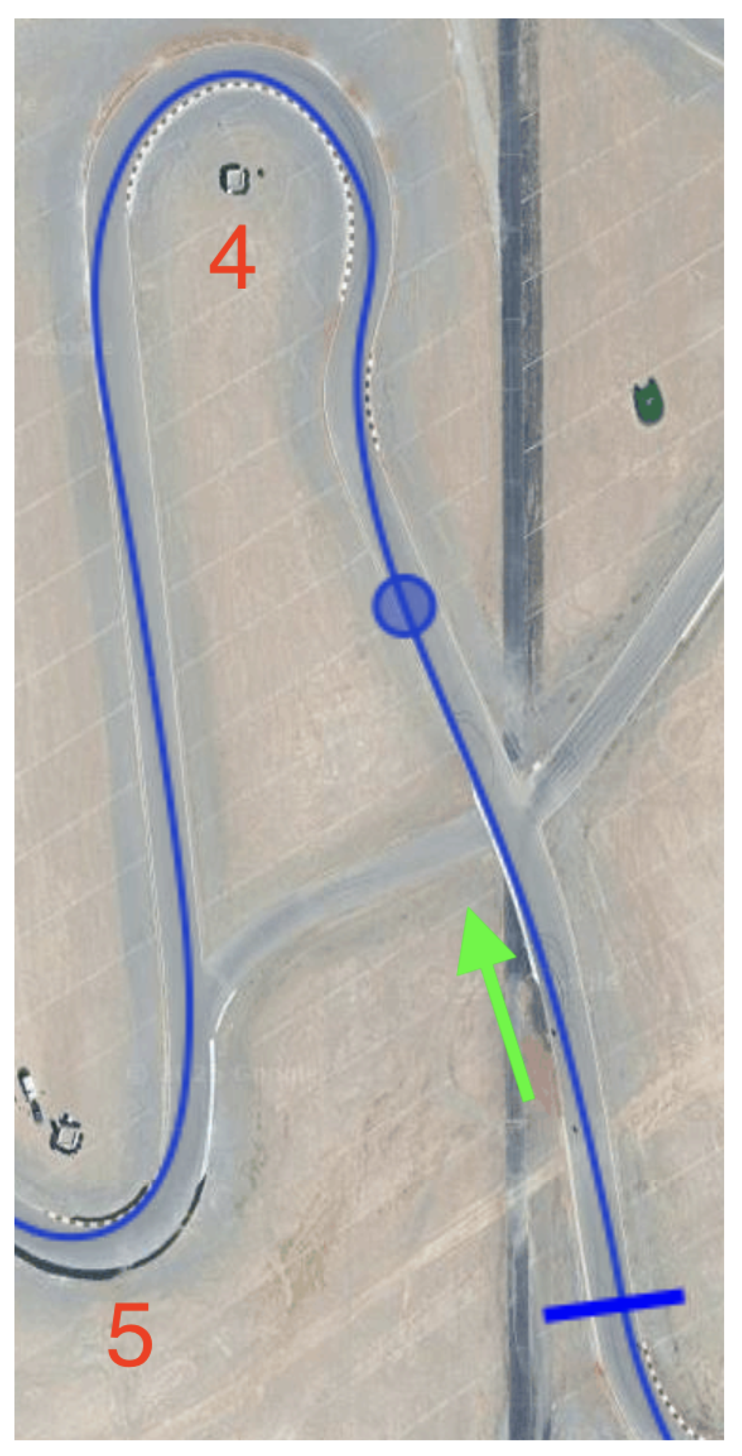
When the tight curved section ends, the path straightens but remains slightly curved, and the vehicle begins building speed, gaining approximately 40 kph as reported by the plot. The corresponding outputs are shown in Figure A3, and the associated track section is shown in Figure A8. The vehicle then reaches the slowest section on the track, Turn 4. As the turn ends, there is a straight leading to Turn 5. The model correctly predicts the driving scenario throughout this sequence.
5.4. Turn 13 - Turn 1
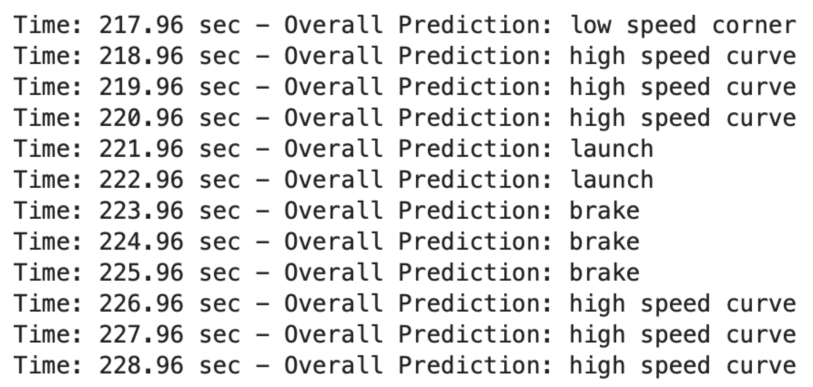
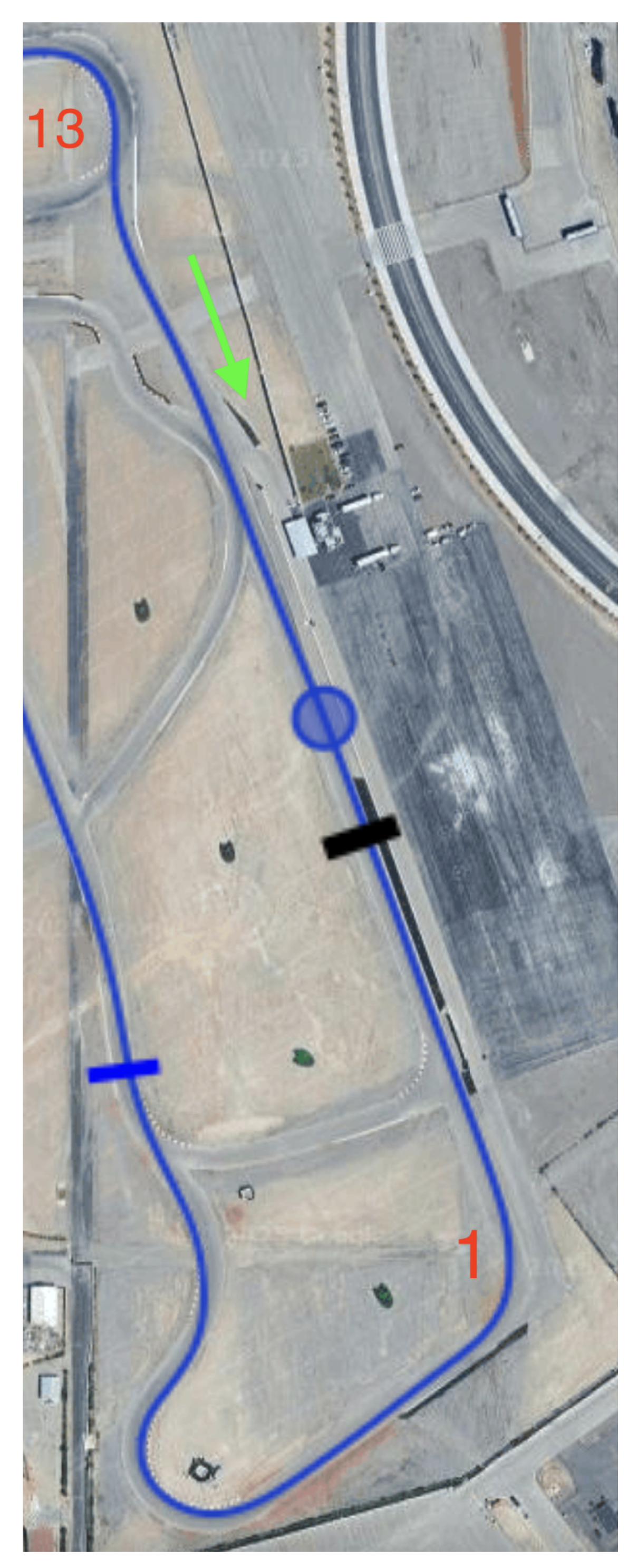
The car continues on the track. Eventually, it returns back to Turn 1. However, the section prior to the first turn, when the vehicle is already on the track, is the longest straight of the course. As a result, the vehicle has been accelerating for a much longer period compared to the entry lap. The vehicle’s speed when approaching Turn 1 on the second lap is now 200 kph instead of 50 kph, necessitating braking to take the corner. The corresponding outputs are shown in Figure A4, and the associated track section is shown in Figure A9. The car exits low-speed Turn 13, enters the straight, and reaches full throttle, which the model registers as a launch event. As the straight nears its end, the driver applies maximum braking to slow the vehicle, which the model reflects by outputting three seconds of brake classifications. Lastly, a series of high-speed curve outputs are seen as the vehicle enters Turn 1, consistent with the earlier lap.
5.5. Exit
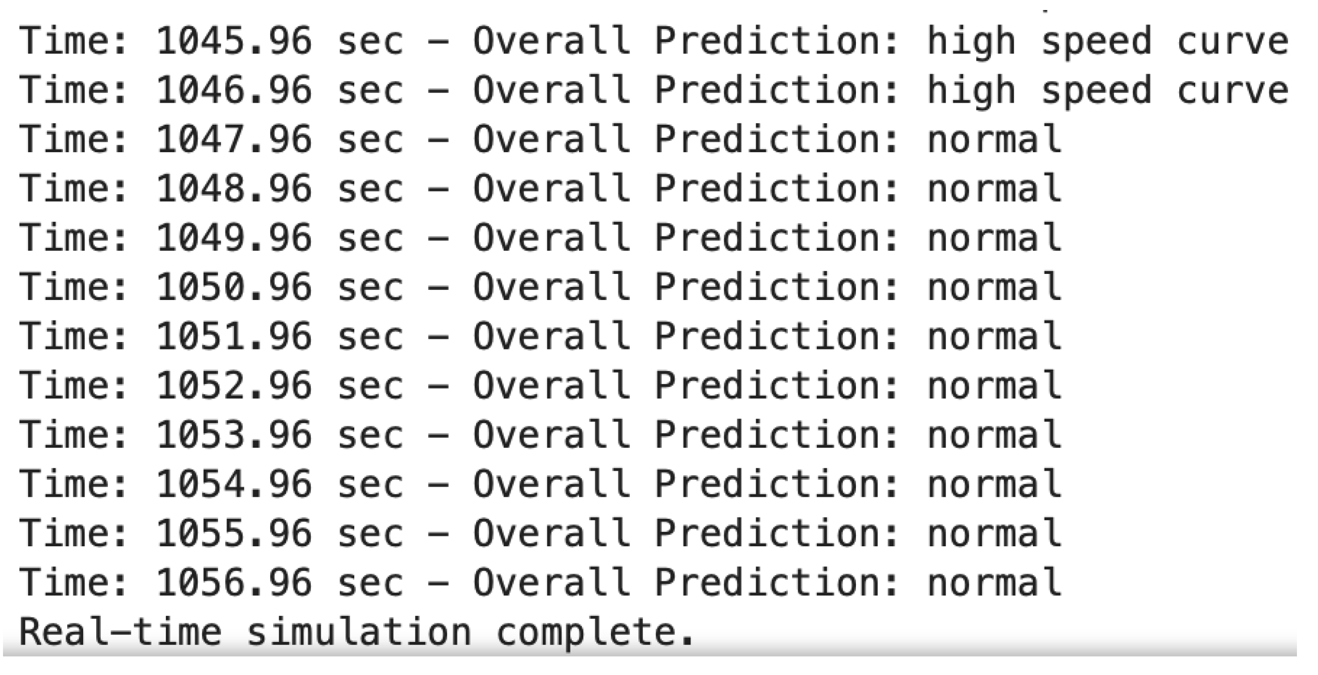
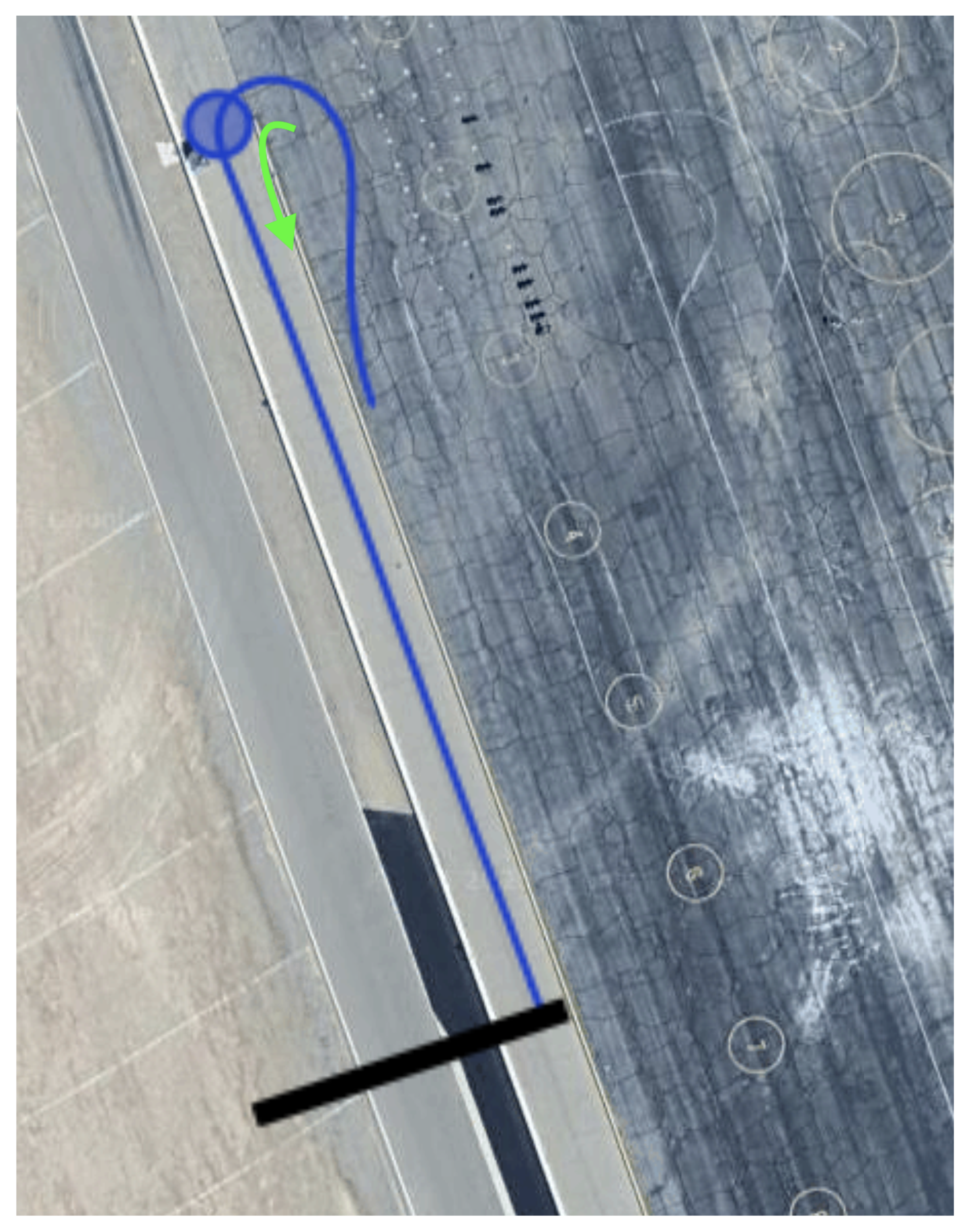
Finally, the last lap of the session is a cooldown lap. At the end of this lap, the vehicles exit the track and enter the parking lot, as shown in Figure A5 and Figure A10. As the car enters a pedestrian area, speed and overall vehicle dynamics are significantly reduced, and the model correctly outputs normal as the grades.
6. Discussion
6.1. Contributions
The inference model accurately recognizes driving scenarios, unlocking an entirely new layer of context-awareness by supplying the controller with rich, real-time information it would otherwise lack [9]. Upon detecting a launch, the rear suspension can be stiffened to prevent squat while still permitting enough weight transfer for improved traction. When braking is identified, the front suspension can be firmed to reduce nose dive and avoid rear traction loss or understeer from overloaded front tires. In low-speed cornering, suspension settings can be tuned to maximize mechanical grip; in high-speed curves, they can be adjusted to preserve aerodynamic stability. When a bump is encountered, the suspension can be softened to prevent bottoming out and maintain tire contact over uneven surfaces. During normal driving, the suspension can be relaxed to enhance ride comfort.
The controller can also adjust its own internal constraints, such as maximum allowable lateral acceleration, steering angle limits, and brake deceleration targets, based on the inferred driving mode, which in turn refines trajectory tracking and stability control [10]. For example, during a high-speed curve, tighter slip and yaw-rate constraints can be imposed to keep the vehicle precisely on its intended line. By continuously tuning both suspension commands and these higher-level constraint sets in tandem, the system not only optimizes ride and handling but also enhances the performance of trajectory control, stability management, and other dependent subsystems under varying real-world conditions, an asset invaluable to autonomous vehicles.
Beyond suspension, the same ML–MPC pipeline can be applied to subsystems such as braking, traction control, and energy management. For instance, consider a fully loaded semi-truck descending a long grade on a hot day: a ML model can continuously grade tire-temperature and brake-pad health from sensor inputs, producing informatics like “tire overheat risk” or “brake fade onset.” The MPC can then tighten deceleration and slip-ratio constraints, modulating engine braking, retarder settings, and service-brake commands, to maintain safe downhill speed without overheating components. Simultaneously, the controller can update its internal limits on allowable brake torque and shift schedules to optimize drivetrain efficiency and prolong component life [11]. In electric or hybrid vehicles, analogous inferences about battery temperature and state-of-charge could tune regenerative-braking profiles [12]. By grading each subsystem’s real-world status and feeding those semantic modes into the optimizer, the approach generalizes effortlessly across diverse vehicle platforms and operating conditions.
6.2. Challenges and Future Work
The inference model may mislabel ambiguous or novel driving conditions, particularly those under-represented in training, leading the controller to apply inappropriate constraint sets. For example, a single model optimized for both performance and everyday driving may struggle to distinguish between certain driving scenarios. One mitigation strategy is to maintain multiple inference profiles (e.g., Sport, Comfort) that can be selected automatically or manually. Another is to experiment with other models such as neural networks, which may improve discrimination when more extensive datasets are available.
Larger sliding windows introduce greater latency, potentially delaying the detection of rapid transitions and compromising control responsiveness. Conversely, overly short windows can yield oscillatory predictions, leading to instability. An appropriate window length must therefore be selected to balance responsiveness and smoothing for the specific application. Alternative methods such as event-driven updates, adaptive windowing, or bespoke weighting schemes can be explored to mitigate this trade-off.
Continuous probability estimation and weighted averaging impose significant computational overhead on Electronic Control Unit (ECU) hardware. Potential solutions include adopting ultra-low-latency inference frameworks, applying model compression and quantization techniques, and deploying dedicated accelerators to ensure real-time performance.
The framework’s accuracy depends on the quality and breadth of labeled data; collecting and maintaining diverse, high-fidelity datasets is laborious and may never encompass every edge case. The system must also be robust to sensor noise and potential malfunctions to maintain reliable performance.
Finally, future work should investigate model predictive or other control architectures that directly leverage the ML-derived inferences to adapt prediction parameters, objective weights, and operational constraints.
7. Conclusion
In this work, a general, data-driven framework was developed and validated to close the loop between real-time machine-learning inference and model-predictive control in vehicle systems. Accelerometer and gyroscope data from five distinct driving maneuvers were used to train a model capable of predicting each maneuver in real time with over 97 percent accuracy. When integrated into a controller, these inferences can be used to tune suspension, or any other subsystem’s parameters to enhance vehicle performance, safety, and component longevity. This framework scales seamlessly, offering a unified, data-driven path toward fully adaptive, self-optimizing automotive control architectures.
Author Contributions
Conceptualization, E.A. and S.L.; Methodology, E.A. and S.L.; Software, E.A.; Validation, E.A. and S.L.; Formal analysis, E.A. and S.L.; Investigation, E.A. and S.L; Data curation, E.A.; Writing—original draft, E.A.; Writing—review & editing, E.A. and S.L.; Visualization, E.A.; Supervision, S.L.; Project administration, S.L. All authors have read and agreed to the published version of the manuscript.
Funding
This research received no external funding.
Data Availability Statement
The data collected and used in this study are openly available at: https://doi.org/10.5281/zenodo.15288740.
Conflicts of Interest
The authors declare no conflicts of interest.
Appendix A
Appendix A.1
Figure A1.
Outputs corresponding to pit lane.
Appendix A.2
Figure A2.
Outputs corresponding to Turn 1 to Turn 3.
Appendix A.3
Figure A3.
Outputs corresponding to Turn 4.
Appendix A.4
Figure A4.
Outputs corresponding to Turn 13 to Turn 1.
Appendix A.5
Figure A5.
Outputs corresponding to exit lap.
Appendix B
Appendix B.1
Figure A6.
Map corresponding to pit lane.
Appendix B.2
Figure A7.
Map corresponding to Turn 1 to Turn 3.

Appendix B.3
Figure A8.
Outputs corresponding to Turn 4.
Appendix B.4
Figure A9.
Outputs corresponding to Turn 13 to Turn 1.
Appendix B.5
Figure A10.
Outputs corresponding to exit lap.
References
- Norouzi, A.; Heidarifar, H.; Borhan, H.; Shahbakhti, M.; Koch, C.R. Integrating Machine Learning and Model Predictive Control for automotive applications: A review and future directions. Engineering Applications of Artificial Intelligence 2023, 120, 105878. [Google Scholar] [CrossRef]
- Wang, L.; Yang, S.; Yuan, K.; Huang, Y.; Chen, H. A Combined Reinforcement Learning and Model Predictive Control for Car-Following Maneuver of Autonomous Vehicles. Chinese Journal of Mechanical Engineering 2023, 36, 80. [Google Scholar] [CrossRef]
- Vu, T.M.; Moezzi, R.; Cyrus, J.; Hlava, J. Model Predictive Control for Autonomous Driving Vehicles. Electronics 2021, 10. [Google Scholar] [CrossRef]
- KW Automotive. In the Spotlight: KW ClubSport 3-Way and KW Variant 4 in the BMW M4. https://blog-int.kwautomotive.net/in-the-spotlight-kw-clubsport-3-way-and-kw-variant-4-in-the-bmw-m4/. Accessed: 3 March 2025.
- Pinho, J.; Costa, G.; Lima, P.U.; Ayala Botto, M. Learning-Based Model Predictive Control for Autonomous Racing. World Electric Vehicle Journal 2023, 14. [Google Scholar] [CrossRef]
- Amalyan, E.; Latifi, S. Machine Learning-Based Grading of Engine Health for High-Performance Vehicles. Electronics 2025, 14. [Google Scholar] [CrossRef]
- RaceBox. RaceBox Mini and Mini S Technical Specifications. https://www.racebox.pro/products/racebox-mini/tech-specs, 2025. Accessed: 4 April 2025.
- Chen, T.; Guestrin, C. XGBoost: A Scalable Tree Boosting System. In Proceedings of the Proceedings of the 22nd ACM SIGKDD International Conference on Knowledge Discovery and Data Mining. ACM, 2016, pp. 785–794. [CrossRef]
- Goel, Y.; Vaskevicius, N.; Palmieri, L.; Chebrolu, N.; Arras, K.O.; Stachniss, C. Semantically Informed MPC for Context-Aware Robot Exploration. In Proceedings of the 2023 IEEE/RSJ International Conference on Intelligent Robots and Systems (IROS); 2023; pp. 11218–11225. [Google Scholar] [CrossRef]
- Assi, M.; Amer, M.; Özkan, B. Adaptive Model Predictive Control of Yaw Rate and Lateral Acceleration for an Active Steering Vehicle Based on Tire Stiffness Estimation. Palestine Technical University Journal of Research 2024, 12, 54–79. [Google Scholar] [CrossRef]
- Lu, X.Y.; Hedrick, J. Heavy-duty vehicle modelling and longitudinal control. Vehicle System Dynamics - VEH SYST DYN 2005, 43, 653–669. [Google Scholar] [CrossRef]
- Ezemobi, E.; Yakhshilikova, G.; Ruzimov, S.; Castellanos, L.M.; Tonoli, A. Adaptive Model Predictive Control Including Battery Thermal Limitations for Fuel Consumption Reduction in P2 Hybrid Electric Vehicles. World Electric Vehicle Journal 2022, 13. [Google Scholar] [CrossRef]
Figure 1.
Process flowchart of the machine learning framework.
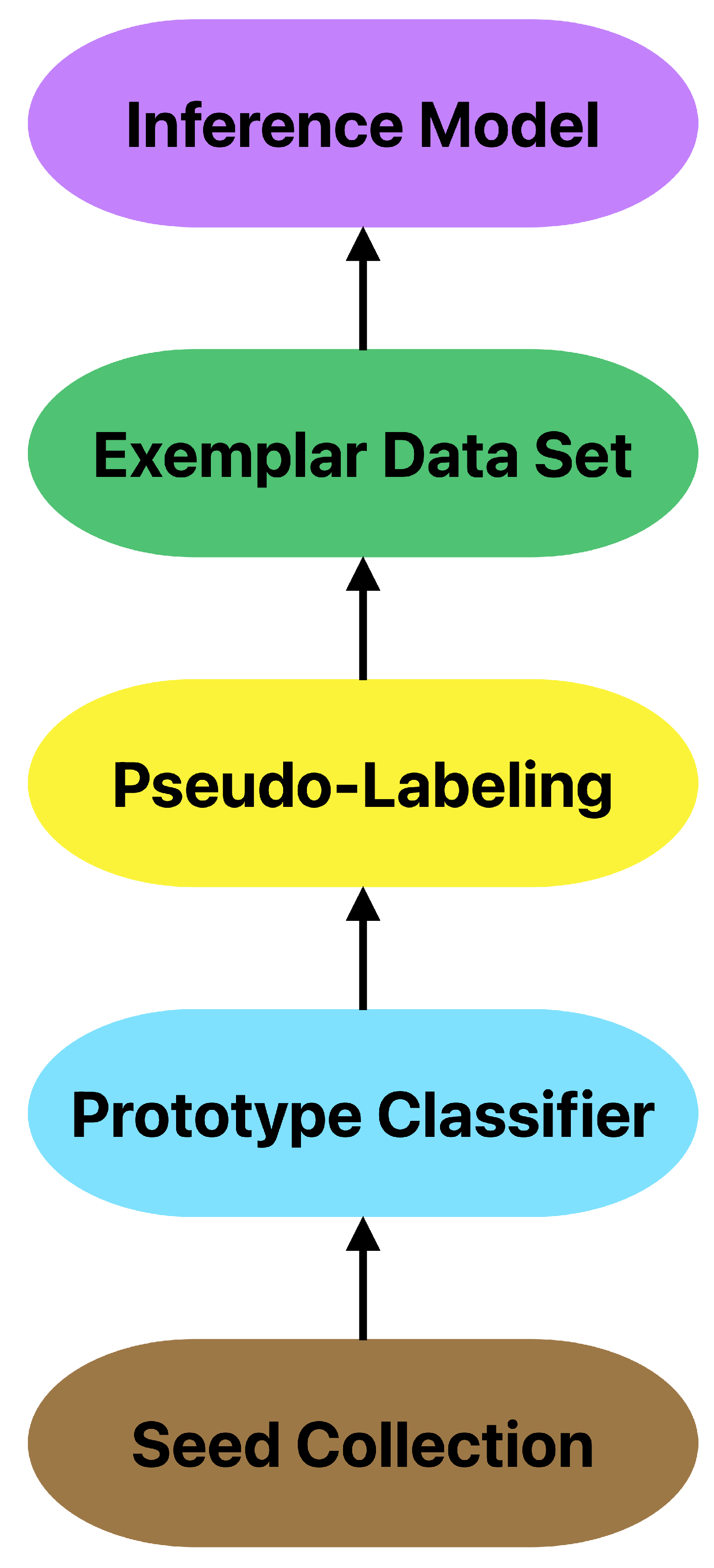
Figure 2.
Unprocessed data from Racebox CSV file.
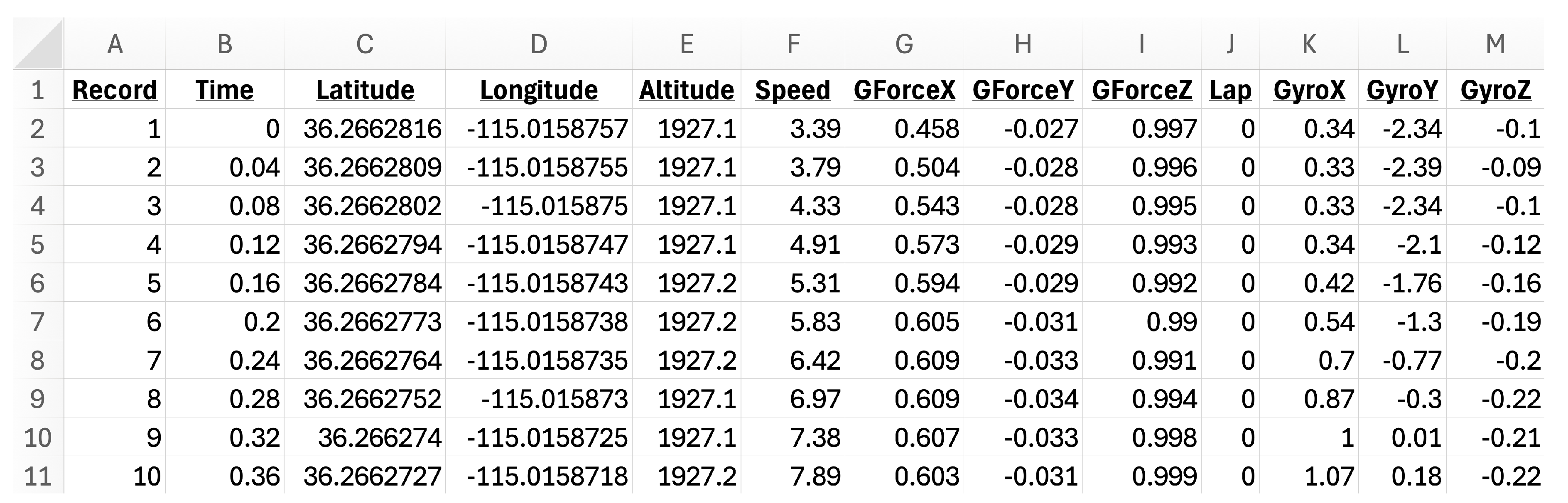
Figure 3.
Processed and labeled seed data.
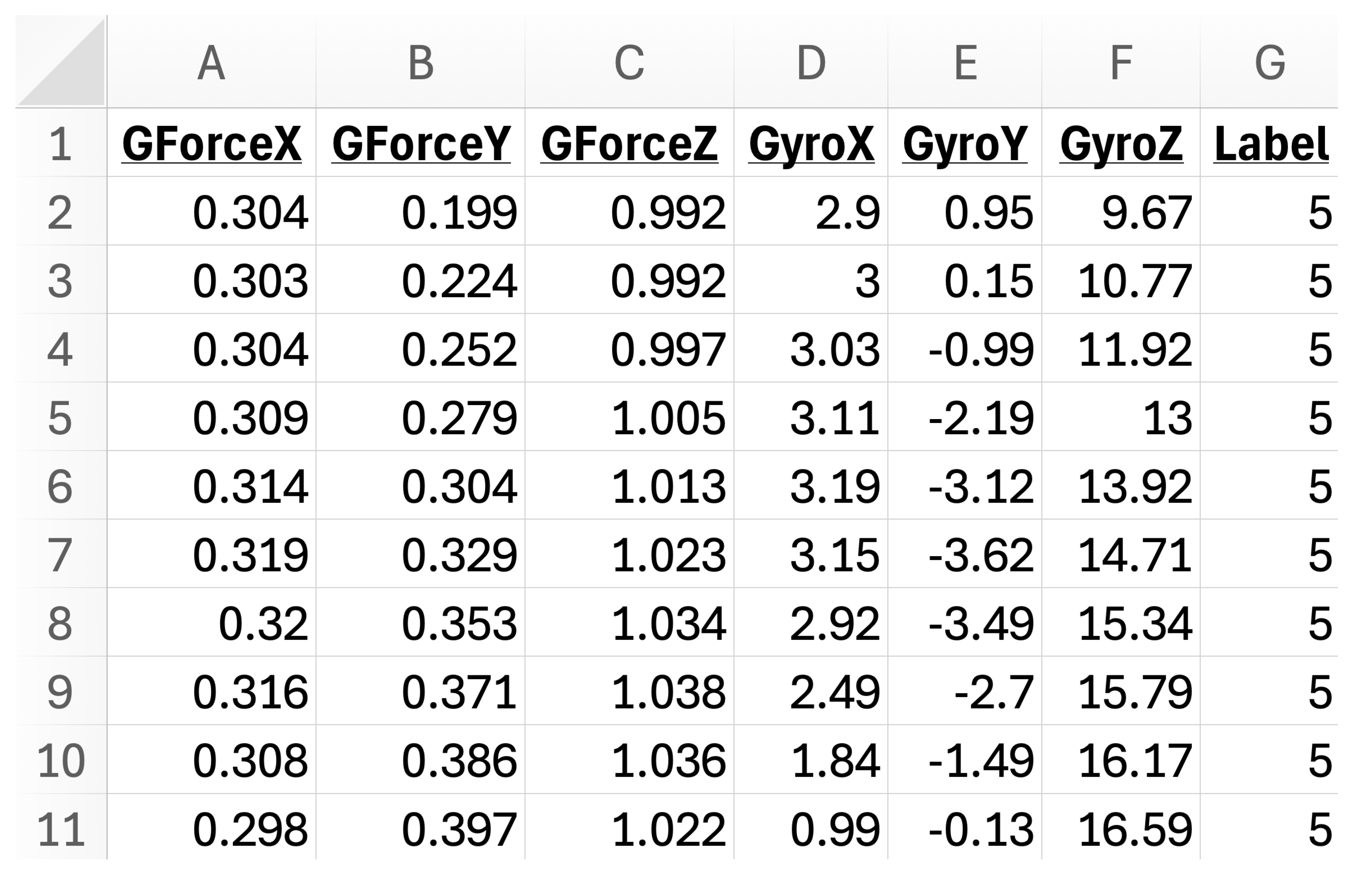
Figure 4.
XGBoost feature importance chart.

Figure 5.
Racebox website time-series plot of a lap.
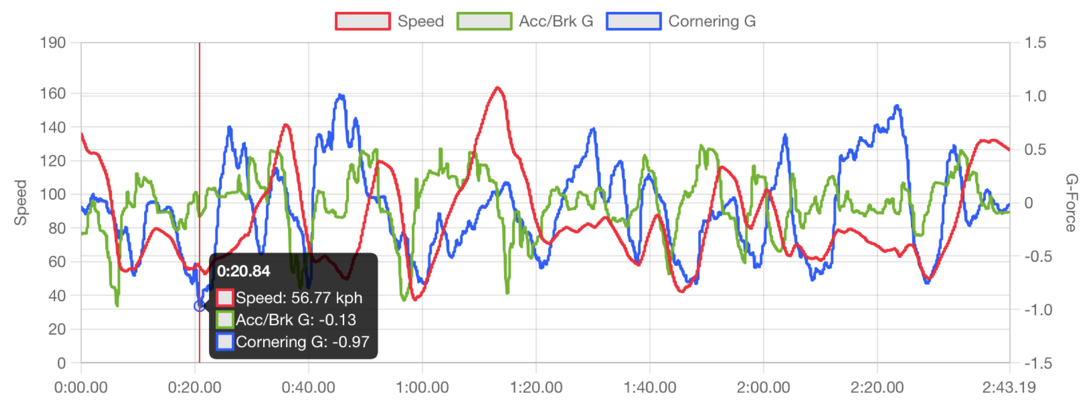
Figure 6.
Racebox website satellite overlay of LVMS Outside Road Course with driven trajectory, annotated with turn numbers and direction of travel.
Figure 6.
Racebox website satellite overlay of LVMS Outside Road Course with driven trajectory, annotated with turn numbers and direction of travel.
Disclaimer/Publisher’s Note: The statements, opinions and data contained in all publications are solely those of the individual author(s) and contributor(s) and not of MDPI and/or the editor(s). MDPI and/or the editor(s) disclaim responsibility for any injury to people or property resulting from any ideas, methods, instructions or products referred to in the content. |
© 2025 by the authors. Licensee MDPI, Basel, Switzerland. This article is an open access article distributed under the terms and conditions of the Creative Commons Attribution (CC BY) license (http://creativecommons.org/licenses/by/4.0/).
Copyright: This open access article is published under a Creative Commons CC BY 4.0 license, which permit the free download, distribution, and reuse, provided that the author and preprint are cited in any reuse.


