
Submitted:
28 April 2025
Posted:
30 April 2025
You are already at the latest version
Abstract
Morphing blades have shown an ability to improve performance in simulations. These simulations show increased performance in Region 2 operating conditions. To improve morphing structures for energy production, this study focuses on the effects of the wake for a flexible wind turbine with actively variable twist angle distribution (TAD). These wake effects influence wind farm performance for locally clustered turbines by extracting energy from the free stream. Hence, the development of better wake models is critical for better turbine design and controls. This paper provides an outline of some approaches available for wake modeling. FLORIS (FLow Redirection and Induction Steady-State) is a program used to predict steady-state wake characteristics. Alongside that section 4 shows different modeling environments and their possible integration into FLORIS. In section 6, we look at the 20 kW wind turbine analysis with previously acquired data from the National Renewable Energy Laboratory’s (NREL) AeroDyn software. The previous study used a genetic algorithm to obtain 9 TAD shapes that maximized aerodynamic efficiency in region 2. In section 6 the analysis compares these TAD shapes to the original blade design regarding the wake characteristics. The project aims to enhance the understanding of FLORIS for studying wake characteristics for morphing blades.
Keywords:
Wind Energy
; Morphing Blade
; Variable Twist Angle
; Wake Model
; NREL
; FLORIS
1. Introduction
According to recent figures the global energy consumption has been increasing over the past few years with current consumption at 2.93x10¹³ kWhs of energy consumed in USA annually [1]. With climate change and volatile fossil fuel prices there has been an increase in the attention towards renewable energy. Wind energy shows potential to provide an alternative to fossil fuels but current utility-scale wind energy infrastructure in the USA only has a capacity to provide 35% of the current energy demand of 107 GW [2]. The International Energy Agency (IEA) has indicated an interest in blade design and control techniques to complement current turbine performance to diversify and optimize energy sources [3]. Current control schemes aim to improve wind capture through gearbox designs and power conversion equipment for variable rotor speed. During partial (Region 2) or full load (Region 3) conditions the aerodynamic efficiency can be affected by blade control through adjusting generator torque and blade pitch [4]. While these efforts are fruitful there is a physical limit, known as Betz limit, that restricts the ability to extract the kinetic energy of the air, regardless of the blade design and control [5]. This limit, based on conservative estimates, caps the maximum efficiency of a turbine to be 59.3%. This is often parameterized as the cp [5]. Industry standard turbine and blade control attempt at maximizing power under isolated unobstructed flow. Turbines are often located in clusters arranged in arrays of rows in close proximity. The rationale behind this is to concentrate them geographically and increase profitability with regards to the wind resources available. The clustering also reduces the maintenance and transportation cost by requiring material to be carried to single local site. Due to an increase in energy demands more wind farms are being built in proximity (±40 km) to one another [6]. This leads to a substantial drawback in the aerodynamic performance of the wind farm due to the induced wake effects. A 209 MW capacity Texas wind farm situated downstream to another wind farm demonstrated power generation losses, due to wake effects, as 184,415±120,930 MWh between the years of 2011-2015, roughly corresponding to $730K±485K annually [7]. Since the upwind farm extracts kinetic energy of the air and hence reduces the velocity and hence momentum of the air the downstream farm will produce less power and revenue [6,8]. Similar concept can be applied to turbines within a wind farm. When the incoming air flows through the upstream turbine it produces a region of separated flow dominated by pressure drag and hence reduces the performance of the downstream turbine. These deficits are quantified as a 20-30% reduction in power relative to unimpeded turbines, increase of 5-10% in fatigue loading for the downstream blades due to an increase in wake turbulence intensity (TI) , and an increase in noise emission from the downstream turbine [6,8,9]. Therefore, it is critical to develop an understanding of the wake effects to extract maximum power out of a wind turbine. Hence quantifying this phenomenon is seen as a motivating factor for this project. The wake characteristics can be affected by techniques such as active wake control by varying turbine characteristics such as tip-speed ratio (TSR), pitch angle and yaw angle. In a previous work by Bingzhen et al. TSR and pitch angle were varied to quantify the performance and the spatial wake evolution of a small-scale wind turbine. It was observed that the larges wind velocity deficit and maximum power coefficient occurred at the optimal TSR value when the TSR was varied. Alternatively, an increase in just the pitch angle did not lead to the largest wind velocity but induced greater effects on wake velocity. Along with that large pitch angles yielded low wind velocity deficit and weak wake TI. Hence the change of the blade’s pitch angle exhibits a greater effect on the wind velocity when compared with controlling the TSR in both near and far wake regions. When increasing the yaw angle, both the wake velocity and TI are reduced, generating an asymmetric wake structure [10]. In another study the two-turbine case was examined to understand the effects on the downstream turbine. Axial induction-based wake control was achieved by using torque control to increase the blade pitch angle and/or reducing the TSR. This study showed an increase in wake velocity, reduction in axial induction factor (AIF), rotor thrust and power production of the upstream turbine while increasing the power production of the downstream turbine [11]. Yaw based wake control of the upstream turbine reduces the wake overlap with the downstream turbine, through misalignment of the incoming flow, thus increasing the power production of the downstream turbine in comparison to the upstream turbine [12]. This technique is known as secondary steering, where turbines work together to build larger vortex-structures, leading to the deformation and deflection of the downstream wake, resulting in an increase in wind farm performance [13,14]. Advancement in blade design, materials and control has led to the progress of turbine performance in a range of environmental conditions, yet current fixed geometry blades, employing torque and blade pitch control, are not optimal across all operational conditions. Current blade stiffness hinders the development of control approaches that enhance wind capture, lessen fatigue loads and improve mechanical and electrical stability, these shortcomings need to be overcome [15]. Variable blade geometry is a new frontier for achieving blade control to improve operation and lifespan [16]. While not a new concept, recent improvements in material and manufacturing technology position morphing blades as an avenue for growth for wind turbine operation and lifespan [17]. A geometrical change in shape as a result of blade actuation or smart materials is referred to as morphing. An example of morphing technology are the flaps on an airplane wing [18]. These morphing blades have been influenced by the ability of birds to adapt to changing environmental conditions to optimize flight path [17,18,19]. These abilities to adapt to changing conditions are particularly suitable for wind turbines that would make them resilient to various forms of forces encountered, making them suitable for a range of inflow conditions when compared to standard fixed blade technology[20,21]. MacPhee and Beyene, validated higher torque, increased cp, and broader operational wind speeds for flexible blade technology when compared to traditional fixed blade counterparts [15]. Conventional control surfaces in wind turbines could exploit adaptability through active twist, camber, chord, and stiffness variations in blade geometry, such as using active tendons [22,23,24]. Studies show that combining active twist and chord extension improves aerodynamic performance by 11% [20]. Similarly, optimizing chord and twist angle distribution enhances the annual energy production (AEP) in small wind turbines [23]. Loth et al. proposed tension cables to distribute equivalent forces between cable and centrifugal loads passively [24]. Morphing blades improve efficiency, reduce vibrations, resist stall, and increase the lift-to-drag ratio. A segmented blade with adjustable pitch angles for each section was studied by Gili and Frulla, who used electric motors and cables to vary twist and enhance lift [25]. Daynes and Weaver demonstrated a flexible flap assembly on a turbine blade that increased lift, reduced drag and regulated power [26]. Wang et al. demonstrated that modifying twist at blade tips and bases in a simplified morphing blades boosts AEP over pitch/stall-regulated designs [16]. Morphing blades have primarily been tested in wind tunnels using small prototypes, with limited fabrication for large-scale applications [21]. This underscores the need for further research to support the IEA vision for advancing this technology [3]. Previous studies developed a design framework for blades with active twist angle distribution (TAD), ensuring an optimal angle of attack along the rotor radius, where the twist angle varies with blade length [27,28,29,30]. This framework, validated using NREL’s AeroDyn software, analyzed twist angles at discrete blade points and identified TAD geometries that maximize operational efficiency. This paper aims to consolidate knowledge on wake effects and integrate aerodynamic analysis of ideal TAD shapes using NREL FLORIS software for wind speeds in Region 2, ranging from cut-in to rated speed in 1 m/s increments. The mechanical design for implementing such blades is also explored. Blade shapes were modeled as a function of wind speed and radial distance from the hub. Using data from the NREL Unsteady Aerodynamics Experiment (UAE) Phase VI, a fixed-speed 20 kW turbine with TAD blades was analyzed to study wake effects. Subsequent sections delve into wake physics (Section 2), wake models (Section 3), simulation software (Section 4), the flexible blade concept (Section 5), and preliminary FLORIS results (Section 6).
2. Wake Aerodynamics
Wake is defined as a region of recirculating flow immediately behind a bluff body or a wave pattern in the downstream fluid generated by a moving object. These flow patterns can be attributed to viscosity, resulting in flow separation, turbulence and density gradients [31]. A static turbine acting as a bluff body creates velocity gradient and shear stress due to the no slip conditions as the fluid moves over the surface. These effects of reduced flow velocity and non-zero shear stress are carried away form the body due to viscous diffusion [32]. These effects of viscous diffusion are carried out at a slow rate, but convection drives them faster creating a thin boundary layer. Which of these competing effects of viscous diffusion and convection are dominant depends on the Reynolds number (Re). A high Re results in a higher rate of downstream convection away from the surface, thus the vorticity generated at the surface are swept back further. At moderate Re the flow separates when it interacts with the body and hence the flow does not have sufficient momentum to go around the body [33]. After flow separation, an adverse pressure gradient develops due to the low velocity and momentum within the boundary layer. When subjected to this adverse pressure gradient, the boundary layer lacks sufficient momentum to overcome it, causing the flow to detach from the surface rather than follow it. With high Re the region of flow separation is reduced due to turbulent mixing bringing higher momentum flow closer to the surface [34]. High Re is also known to produce von Kármán Street vortex a form of unstable flow. This appear in the form of vortex shedding that arises from instabilities in attached eddies, when flow in the shear layers is slower than the surrounding flow, hence rolling into vortices. The resulting oscillating forces, characterized by the Strouhal number cause unsteady loading on structures [31,33]. A rotating propellor in uniform flow produces various vortex structures by the hub, nacelle, tower and the blade tips due to the turning blades [35]. These wake formations can be categorized into two regions the near-wake and the far-wake region. In the far wake region, the geometry of the turbine no longer plays a significant role since the helical vortex structure formed in the near wake structure breaks down due to instabilities. The geometry of the wind turbine dominates the vortex structures seen in the near wake regions since this is dependent upon the rotor radius and the wake growth rate. As the blades rotate the vortices from the tip and the root start shedding [34,36]. These tip vortices, rotating in the opposite direction to the rotor, are located in the shear layers that form, between the near and far wake regions, due to the difference in velocities between the inside and the outside air. This region increases in thickness as it moves downstream ultimately reaching the wake axis. These highly turbulent shear layers lead to momentum transfers due to turbulent mixing and hence the velocity deficit is reduced as the wake moves downstream. Both velocity deficit and enhanced turbulence are used to characterize this turbine wake. Velocity deficit leads to reduced power output from the downstream turbine while the enhanced turbulence results in dynamic loading (fatigue) which reduces the blade lifespan. This velocity deficit recovers downstream as the turbulence mixing occurs and has a Gaussian shaped profile[37]. Immediately behind the wind turbine, tightly wound helical vortices form from the blade tips, roots, and nacelle, with streamwise vortex structures concentrated at the center. Further downstream, wake instability caused by expansion and vortex interactions destabilizes the helical structure. Tip vortices lose uniform vorticity, and root vortices unwind, forming counter-rotating vortex pairs that drift away from the turbine axis. These two vortex structures interact further downstream but do not alter the flow [38]. These vortices, along with turbulence from the nacelle, tower, and boundary layers, create a significant velocity deficit immediately downstream, which recovers gradually in the far wake. High turbulence intensity is concentrated in regions of strong vorticity, while areas outside this zone experience lower turbulence intensity. However, unsteady loads on downstream turbine blades, caused by vortex structures, reduce power output and induce fatigue, impacting turbine performance.
3. Wake Models
These models take the interplay between the upstream and downstream turbine when it comes to wake. The upstream turbine is considered as an isolated system but the effect of wake from the upstream turbine changes the initial conditions of the downstream turbine. FLORIS models are classified by velocity deficit, wake combination, deflection and added turbulence [39]. Velocity deficit models take the effect of reduced velocity from the upstream turbine into account. This reduced velocity affects the power output of the downstream turbine. Wake deflection models address horizontal or vertical displacement in the upstream turbine, due to free stream and turbine misalignment, based on the model used [40]. The wake combination models demonstrate how resulting velocity profile are combined with each other, addressing the wake super position concept. The added turbine models compute the added turbulence from the turbine interaction with ambient turbulence. These numerical models can involve differential equations solved from fluid, turbine dynamics governing equations, analytical equations from mass or momentum conservation or data driven reduced order models through CFD data [41]. The various models that are available for wake modelling alongside their key features, limitations and their mathematical representation are seen in the section below.
3.1. Jensen Model
This model uses an actuator disc model with linear wake expansion and tunable wake decay constant [42]. It is simple and computationally inexpensive, widely adopted in FLORIS. The computation time for this model in FLORIS is 0.0018 seconds [43]. However, it ignores added turbulence from turbine operations [44].
3.2. Multi-Zone Model
The Multizone model divides the wake into three zones (near-wake, far-wake, and mixing-wake), each with its own linear expansion factors [45]. The model is computed in 0.0019 seconds in FLORIS [43]. The wake zones of each upstream turbine, j, is combined to fine the effective velocity of the downstream turbine i [44]. The tuned scaling factor (MU,q) causes the velocity of the outer zones to recover faster than the inner zones. It accounts for partial wake overlap but is sensitive to tuning parameters and ignores added turbulence effects.
3.3. Jimenez Model
Jimenez model simulates yaw-induced wake deflection with small angle approximations and uniform wake velocity [46]. It effectively accounts for yaw effects but oversimplifies flow dynamics, leading to errors in far-wake estimations. Using small angle approximations, the skew angle (defined as the angle between the wind direction and skew direction) is defined as.
Using this skew angle and the Taylor series expansion the amount of deflection by yaw misalignment in the spanwise (y-direction) is determined as [44].
3.4. Bastankhah and Porté-Agel Model
The Bastankhah and Porté-Agel model is based on RANS equations, it separates wake sections by streamwise position to account for wake deflection and steering [47]. FLORIS calculates the axial induction factor in terms of ct, irrespective of the sub model chosen, defined below, where is the flow skew angle in terms of the rotor axis [40]. It is accurate for wake steering but limited by simplified RANS analysis assumptions.
The total deflection of the wake as a consequence of the wake steering is seen in the equations below, where is constant in terms of the potential core of uniform velocity , and the wake growth rate is linearly proportional to the incoming TI.
3.5. Gaussian Model
The model employs a Gaussian velocity deficit distribution based on self-similar shear flow theory [47]. Due to its simplified NSE and free shear flow theory, the computational time is low at 0.0025 [43]. It is computationally efficient and models lateral/vertical wake meandering but is limited by simplified Navier-Stokes assumptions. In the far-wake region, an analytical 3D velocity deficit expression is presented
is the wake deflection and the subscript “0” refers to the initial values at the start of far-wake which is dependent on the turbulence intensity . The velocity distribution, in the y and z direction, of the lateral and vertical wake width () are defined in the equations below.
3.6. Curl Model
The model captures curled wake effects under yaw using elliptic vorticity distribution and parabolic PDE solutions. Provides detailed modeling of wake deflection but at a higher computational cost (1.6 seconds in FLORIS) and requires numerical methods [43]. The equations below describe the downstream evolution of the wake deficit ( ). Here and are assumed to be zero, hence there is a single parabolic partial differential equation, that can be solved as a marching problem [48]. Martínez-Tossas et al suggested possible improvements to the model noting the differences between the model and the LES simulations [49].
3.7. Gauss-Curl Hybrid Model
As the name suggests the model combines Gaussian and Curl models to improve wake deficit and deflection accuracy while maintaining low computational cost [48]. The model is effective especially when it comes to addressing the discrepancies of Gaussian model’s ability to estimate downstream power using field data. The GCH solves this by incorporating yaw-added recovery and secondary steering for appropriate wake deficit and deflection to match field data [14].
3.8. Larsen Model
Exclusive to the MATLAB version of FLORIS the Larsen model assumes symmetric turbulent wake and uses Prandtl’s turbulent boundary layer equations in cylindrical coordinates [40]. Accurate for symmetric wakes but limited to specific turbulence assumptions like the first or second-order approximations of RANS assuming steady and self-similar flow for velocity deficit profile [50].
3.9. Wake Combination Models
The model combines wakes using velocity or kinetic energy summation methods such as Freestream Linear Superposition (FLS), Max Velocity Deficit, or Sum of Squares Freestream Superposition (SOSFS). Not fully developed and sensitive to flow field assumptions. FLS simply adds the upwind flow field and the wake flow field to generate the velocity caused by the interaction of these flow fields.
Maximum wake velocity deficit simply selects the maximum of the two points between the base flow field and the wake field.
SOSFS uses the Pythagorean equations to return the resulting sum of squares velocity of the two fields
3.10. Added Turbulence Models
These models, simulate turbulence from turbine operation and ambient conditions. Models like the Gaussian model and the Crespo Hernandez model take ambient conditions into account factors like the atmospheric shear, veer, changes in TI through field measurements and the anisotropy of the wake and atmospheric flow.
3.10.1. Gaussian Model
The Gaussian model links ambient TI to wake expansion using empirical relations seen below [51,52].
The additional turbulence generated, and the ambient conditions are computed using the redefined added turbulence equations seen below, where the number of turbines is represented by N, with. N = 1 indicates the strongest wake effect on the turbine being evaluated [53]. This model relies on the linear wake expansion model and the six tuning parameters (,, , , , ).
3.10.2. Crespo Hernandez Model
This model computes the additional variability through least squares fitting to relate the turbulence kinetic energy to the standard deviation of the wind direction assuming similarity between the anisotropy of the wake to be similar to the atmospheric flow [54].
With, between 5 to 15, between 0.07 and 0.14 and a between 0.1 and 0.4. The FLORISE software only uses the added turbulence in the far wake region [40,54].
4. Modeling Tools
This study was focused on the aerodynamic modelling of turbine blades. These models are of varying accuracy, categorized as steady state, control oriented models, medium fidelity models and high-fidelity models [55]. The steady state models predict time averaged properties and hence temporal dynamics are ignored. These models are computationally inexpensive but only provide quantities averaged over periods of 5-10 minutes. Control oriented models capture the dominant flow characteristics on second scale. These tend to be computationally more expensive than the steady state models. Medium fidelity models are less computationally expensive than the high fidelity LES models and hence are suitable for controller testing while losing out on some of the finer spatial and temporal resolution available with the high-fidelity simulations. In the following section we will see the various modelling tools available for these simulations and their uses and limitations.
4.1. FLORIS
FLORIS is an open-source software designed to optimize wind farm energy production and simulate wake interactions using reduced-order engineering models. Developed originally in MATLAB as FLORISSE by Delft University of Technology and later extended in Python through collaboration with the National Renewable Energy Laboratory (NREL), it provides a low-fidelity yet computationally efficient framework for analyzing wind farm performance [56,57]. This study focuses on the Python version of FLORIS, although a comparison with the MATLAB version is presented later in Section 4.2. FLORIS employs steady-state, nonlinear wake models to predict time-averaged flow fields and turbine power outputs. These models optimize yaw misalignment to enhance wind farm performance while maintaining low computational costs (≤1 second for 100 turbines) [43]. The software uses parameterized thrust and power coefficients, requiring consistent hub heights for turbines but not modeling wake dynamics explicitly [41]. The framework necessitates user-defined inputs in a JSON format, including turbine specifications, wake model parameters, and farm-level flow conditions, such as wind direction, velocity, turbulence intensity, and shear factor [39].
Figure 1.
FLORIS architecture.
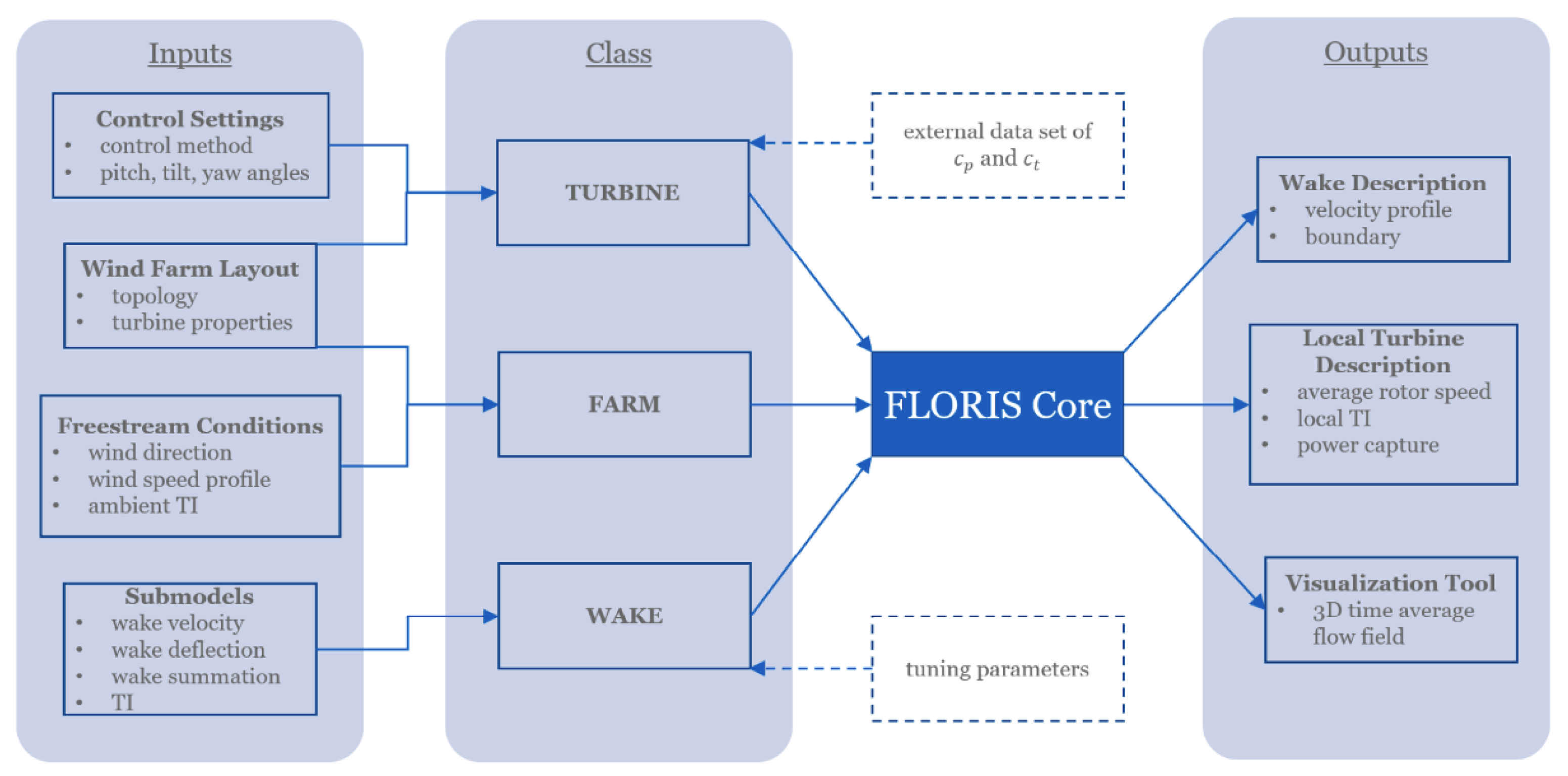
Key features of FLORIS include its object-oriented architecture, which facilitates easy customization, integration with high-fidelity tools (e.g., SOWFA, OpenFAST), and compatibility with aerodynamic codes such as CC-Blade and WISDEM [39,58]. For example, CC-Blade outputs turbine-specific power and thrust coefficients, which FLORIS uses to simulate yaw-aligned and misaligned conditions [44]. Although FLORIS performs well under steady-state assumptions, it lacks the ability to capture transient dynamics or ground effects, and the accuracy depends on properly tuned wake and turbulence parameters [47,58]. Integration with high-fidelity tools like SOWFA and OpenFAST has been explored to address FLORIS’s limitations. SOWFA simulations, though computationally intensive, provide tuning inputs for FLORIS, enabling better insights into wake physics under specific scenarios, such as aligned turbines with and without yaw [59]. OpenFAST, on the other hand, can supply turbine coefficients and axial induction factors derived from its AeroDyn module, allowing FLORIS to model region-3 turbine operations [58]. Recent advancements include incorporating the Gaussian Wake Model (GWM) into the OpenFAST framework, enhancing the description of wake dynamics through real-time calculations of thrust coefficients and axial induction factors [59]. Despite its advantages, FLORIS exhibits some limitations, such as discontinuities in wake velocity across the rotor plane and inner wake zone derivatives, which are inherent to most steady-state models. However, these issues minimally impact overall results [58,60]. Future updates aim to address these limitations by incorporating local effects, advanced turbulence modeling, analytic gradients for optimization, and deeper integration with tools like CC-Blade and WISDEM [43,48].
4.2. FLORISSE
Developed by the Delft University of Technology FLORISSE is a MATLAB version of FLORIS that has a similar architecture [61]. While these two versions share many similarities they wont be capable of converging onto a single solution given the same initial parameters due to the the errors common amongst numerical models [40]. This MATLAB version has several inputs spread across different input files. It is also noteworthy that FLORISSE does not have ability to implement dynamic control.
4.3. OpenFAST
Fatigue, Aerodynamics, Structures, and Turbulence (FAST) is a multi-physics tool developed by NREL to predict wind turbine power performance and structural loads. OpenFAST, its supported version, incorporates additional physics to simulate wind farm wakes and turbine dynamics, providing high-fidelity wake modeling and medium-fidelity turbine-level analysis [62]. It achieves computational efficiency, making it suitable for iterative and probabilistic design [55]. When comparing OpenFAST with FLORIS, notable differences emerge. FLORIS produces smooth wake velocity profiles due to its steady-state models, while OpenFAST results are influenced by turbulent wind conditions. A study by CL-Windcon demonstrated these differences, showing FLORIS predicts minimum velocity at the wake center, increasing outward, whereas OpenFAST’s velocity results depend on axial induction factors across the blade sections ][41]. OpenFAST reveals no blade effects at the hub, and its wake velocity aligns more closely with incoming wind.
Additionally, OpenFAST provides smoother transitions in velocity profiles across the rotor diameter, whereas FLORIS exhibits abrupt changes at wake boundaries. This discrepancy highlights FLORIS’s limitations, including discontinuities. While advanced wake models like Porté-Agel’s could address these issues, the Jensen wake model used in FLORIS restricts wake shape adjustments and recovery factor accuracy.
4.4. SOFWA
SOWFA, developed by NREL, is a high-fidelity simulation tool for modeling time-dependent turbulent atmospheric flows and turbine-wake interactions. Built on OpenFOAM and OpenFAST, it integrates ABL dynamics, turbine aerodynamics, and flow control systems [63]. SOWFA requires both OpenFAST and OpenFOAM for operation, with turbine wakes modeled via the actuator line method. The LES model samples velocities along actuator lines and returns them to OpenFAST, where BEM theory computes aerodynamic forces. These forces are fed back to the LES solver and applied as body forces in the momentum equation, resolving rotor wakes and vortices. OpenFOAM simulates the ABL, driven by pressure gradients calculated through momentum balance. Unlike FLORIS, SOWFA can potentially incorporate pressure gradient analysis, which is critical for wake modeling [55]. SOWFA configurations include OpenFOAM and AeroDyn input files, enabling precise aerodynamic modeling suited for this study [62,63]. In conjunction with this XFOIL and QBlade, developed by Mark Drela at MIT, can be used to design custom airfoil shapes [64]. These Output files can be used with AeroDyn/FAST for analysis which can then be used as input for FLORIS later [65].
5. Flexible Blade Concept
The concept for the flexible wind turbine blade has been seen in the author’s previous work and in Figure 2 [27,28,29,30]. This design includes a rigid spar, surrounded by blade segments mounted in a series and a nonstructural flexible skin. The pitch motor rotates the spar to change the blade angle and multiple actuators provide finer adjustments.
Unlike the rigid blade design, where the twist angle varies along the blade, in the proposed design the twist angle () is a function of the radius (r) and wind speed (u).
Since the blade root moves, the absolute local twist angle is found by summing the spar angle (), and the local twist angle () seen in Figure 3.
The Applications to the design and control of the above-mentioned concepts were done in the author’s previous work. The analysis employed the Aerodyne software and an iterative search algorithm to obtain a set of ideal TAD shapes for the steady shape operation in Region 2 wind speeds. The power coefficient seen in eq. 38 below is optimized at each cross section of the blade. A mechanical design also establishes the techniques to get these TAD shapes and the required optimal actuator positions.
This procedure to find the optimal TAD shapes for each rated wind speed can be seen in the Figure 4 below.
6. Results and Discussion
The previously mentioned TAD design framework was focused on maximizing efficiency in region 2. The results in this section expand upon the former framework by implementing AeroDyn and FLORS wake models to demonstrate effects of wake. For this study a 20 kW wind turbine similar to the one used in the NREL UAE Phase VI turbine study is used. The characteristics for this turbine are listed in Table 1, this performance data has been certified by the NREL [66]. This simple system is suitable for studying the blade twist angle. Along with that this turbine model has been used in other studies, providing us with suitable benchmarks [16,66].

Table 1.
NREL UAE Phase VI Turbine Characteristics.
| Rating | 20 kW |
| Rotor Orientation, Configuration | Upwind, 2 Blades |
| Blade Airfoils | S809 |
| Control | Fixed-Speed |
| Rotational Speed | 72 rpm synchronous speed |
| Cut-in, Rated, Cut-out Wind Speed [m/s] | 3.0, 13.5, 25.0 |
| Rotor, Hub Diameter [m] | 4.6, 0.429 |
| Hub Height [m] | 12.192 |
| Blade Pitch [°] | 2-14 |
| Tilt, Yaw Angle [°] | 0.0 |
The FLORIS simulations seen require the and values for the specific TAD shapes found previously. The AeroDyn was used to study the aerodynamic response of the blades and extract the necessary data. AeroDyn implements a quasi-steady BEM theory [67]. Due to its reliability and fast computational speed BEM is a common method for evaluating these parameters [68]. While reliable BEM breaks down at high values of AIF and does not take the effects of vortex shedding for blade tip and hub into account. AeroDyn implements Prandtl’s tip loss and hub loss, Glauert, and skew wake to tackle these short comings. The AeroDyn model simulates each unique TAD between the speeds of 5 m/s to 10 m/s to obtain the blade performance parameters. Once all the TAD shapes were simulated using pitch control to find the maximum as a function of the pitch angle with a constant rotor speed of 72 rpm for each wind speed. These and values for different wind speeds are seen in Table 2 below. These will be used as input data for FLORIS.
Table 2.
FLORIS Input Table.
| [m/s] | Original | TAD #1 | TAD #2 | TAD #3 | TAD #4 | TAD #5 | TAD #6 | TAD #7 | TAD #8 | TAD #9 | ||||||||||
| 5 | 0.447 | 0.817 | 0.464 | 0.851 | 0.460 | 0.841 | 0.458 | 0.833 | 0.451 | 0.829 | 0.447 | 0.822 | 0.442 | 0.816 | 0.435 | 0.803 | 0.424 | 0.787 | 0.423 | 0.786 |
| 6 | 0.484 | 0.793 | 0.486 | 0.814 | 0.489 | 0.811 | 0.487 | 0.803 | 0.482 | 0.798 | 0.483 | 0.795 | 0.481 | 0.789 | 0.478 | 0.777 | 0.471 | 0.770 | 0.470 | 0.765 |
| 7 | 0.435 | 0.617 | 0.432 | 0.627 | 0.437 | 0.627 | 0.440 | 0.626 | 0.436 | 0.624 | 0.434 | 0.622 | 0.433 | 0.617 | 0.431 | 0.609 | 0.427 | 0.601 | 0.427 | 0.599 |
| 8 | 0.370 | 0.490 | 0.361 | 0.496 | 0.368 | 0.494 | 0.371 | 0.494 | 0.377 | 0.512 | 0.371 | 0.494 | 0.370 | 0.491 | 0.369 | 0.486 | 0.366 | 0.482 | 0.365 | 0.479 |
| 9 | 0.314 | 0.401 | 0.300 | 0.409 | 0.303 | 0.403 | 0.312 | 0.402 | 0.314 | 0.405 | 0.315 | 0.407 | 0.315 | 0.403 | 0.314 | 0.397 | 0.312 | 0.395 | 0.312 | 0.393 |
| 10 | 0.268 | 0.336 | 0.253 | 0.342 | 0.258 | 0.339 | 0.261 | 0.332 | 0.267 | 0.336 | 0.268 | 0.338 | 0.270 | 0.338 | 0.269 | 0.334 | 0.268 | 0.331 | 0.268 | 0.330 |
| 11 | 0.231 | 0.286 | 0.216 | 0.291 | 0.221 | 0.292 | 0.220 | 0.279 | 0.228 | 0.284 | 0.229 | 0.289 | 0.231 | 0.286 | 0.233 | 0.286 | 0.233 | 0.284 | 0.232 | 0.282 |
| 12 | 0.200 | 0.245 | 0.187 | 0.255 | 0.193 | 0.253 | 0.188 | 0.248 | 0.196 | 0.240 | 0.199 | 0.248 | 0.200 | 0.248 | 0.203 | 0.246 | 0.204 | 0.247 | 0.204 | 0.246 |
| 13 | 0.174 | 0.212 | 0.164 | 0.223 | 0.170 | 0.222 | 0.165 | 0.216 | 0.169 | 0.208 | 0.173 | 0.216 | 0.175 | 0.216 | 0.178 | 0.215 | 0.180 | 0.216 | 0.180 | 0.215 |
Table 3.
Percentage Change in and for Different TAD Configurations.
| [m/s] | TAD #1 | TAD #2 | TAD #3 | TAD #4 | TAD #5 | TAD #6 | TAD #7 | TAD #8 | TAD #9 | |||||||||
| % | % | % | % | % | % | % | % | % | % | % | % | % | % | % | % | % | % | |
| 5 | 3.83 | 4.11 | 3.09 | 2.85 | 2.53 | 2.48 | 1.05 | 1.38 | 0.00 | 0.50 | -1.01 | -0.17 | -2.53 | -1.81 | -4.99 | -3.78 | -5.26 | -3.82 |
| 6 | 0.35 | 2.70 | 1.05 | 2.33 | 0.60 | 1.27 | -0.37 | 0.64 | -0.19 | 0.34 | -0.68 | -0.40 | -1.24 | -1.91 | -2.58 | -2.83 | -2.89 | -3.52 |
| 7 | -0.53 | 1.59 | 0.64 | 1.62 | 1.13 | 1.36 | 0.21 | 1.04 | -0.18 | 0.70 | -0.41 | -0.02 | -0.81 | -1.38 | -1.75 | -2.64 | -1.86 | -2.95 |
| 8 | -2.62 | 1.20 | -0.62 | 0.92 | 0.24 | 0.90 | 1.76 | 4.45 | 0.08 | 0.73 | 0.00 | 0.29 | -0.46 | -0.90 | -1.24 | -1.67 | -1.40 | -2.22 |
| 9 | -4.52 | 1.89 | -3.63 | 0.35 | -0.76 | 0.27 | -0.22 | 0.82 | 0.13 | 1.30 | 0.03 | 0.45 | -0.10 | -1.00 | -0.64 | -1.47 | -0.86 | -1.97 |
| 10 | -5.71 | 1.90 | -3.92 | 0.92 | -2.46 | -1.10 | -0.52 | 0.12 | -0.04 | 0.65 | 0.63 | 0.62 | 0.37 | -0.57 | 0.11 | -1.58 | -0.07 | -1.90 |
| 11 | -6.29 | 1.96 | -4.29 | 2.31 | -4.85 | -2.21 | -1.08 | -0.46 | -0.74 | 1.16 | 0.30 | 0.28 | 1.08 | 0.11 | 0.87 | -0.39 | 0.69 | -1.09 |
| 12 | -6.44 | 4.04 | -3.50 | 3.35 | -5.89 | -1.02 | -2.30 | -1.96 | -0.70 | 1.10 | -0.35 | 1.14 | 1.40 | 0.37 | 1.90 | 0.69 | 1.70 | 0.29 |
| 13 | -5.68 | 4.99 | -2.53 | 4.76 | -5.45 | 1.93 | -3.21 | -2.26 | -0.46 | 1.60 | 0.34 | 1.74 | 1.95 | 1.22 | 3.04 | 1.79 | 3.27 | 1.46 |
Once this input from the AeroDyn software was extracted the FLORIS simulations were generated with the previously mentioned python version of FLORIS 2.2.0. The Gaussian wake model was used for these simulations, the parameters and of the model determine the linear relationship between the TI and the Gaussian wake shape. A common assumption is to assume a constant growth rate for simplification. A decimal percent measure was used to define the TI, noting that FLORIS is not suitable for TIs over 0.14. The wind shear is used to define the vertical velocity profile with a shear factor of 0.12. the blade pitch of the turbine can also be specified per the FLORIS reference manual but has not been incorporated in the current study but is being planned in future use [60]. These simulations were constructed for all 9 TAD shapes and the original blade design. For a single turbine the velocity deficit is evaluated by measuring the horizontal cut-plane of the flow at the hub height. Since the different blade profiles contain significant overlap making it hard to separate the distance at which the velocity recovers 99% of the inlet velocity is observed. These distances, in meter, are seen in Table 4 below.
The percentage change relative to the baseline is quantified and seen below in Table 5. Only the profiles that showed a decrease in velocity recovery distance is seen below as a negative percentage value. Only TAD #7-9 are seen to have a better velocity recovery.
The wake interactions between the upstream and downstream turbine were also simulated together to understand the effect on the power production. Figure 5 shows the wind farm layout with the turbines spaced at 5D since this is a common minimum distance for turbines.
The power generated from this upstream and downstream turbine can be seen in Table 6, Table 7 and Table 8. When simulating these turbines negative power output is seen due to hysteresis, where the turbine properties lag behind its changes. This can be seen at the cut in and cut-off speed. From these results the TAD #1 is the most efficient at start up with the lowest cut-in value but is not optimal for other wind speeds. TAD #9 is better for rated speed due to its higher power performance. This data suggests that the flexible blades are most useful near the cut-in and rated speed proven by the evidence that the power coefficient increased by 3.38% and 3.27% for TAD #1 and 9 respectively.
To better understand these effects the percentage change of in the power output is seen in Table 9, Table 10 and Table 11. These tables show the blades that or of most significance. Therefore TAD #3 and #6-8 have the highest increase in upstream power for a broad range of region 2 conditions. TAD #3 improves performance in the startup speeds. TAD #6-8 perform better at higher speeds. In the downstream turbines TAD #1-4 outweigh the power generation of the fixed blade design in early start up, and TAD #6-9 have better function closer to the rated speeds.
Wind direction is an important factor is assessing wake effects. The Win direction can affect the placement and the orientation of the wake cones. To assess this a new layout with turbines arranged synchronously in a row are seen in Figure 6. A reference turbine is included that is unaffected by nearby turbines while the control and test turbines are present to assess the downstream effects of wake. The energy wake loss module in FLORIS was used to calculate the balanced wake loss. This is the total difference in energy production when compared to the reference turbine [69,70]. The formula for this can be seen below in Eq. 38.
The term is used to measure this effect of wake, and these calculations are done by averaging the wake loss for each wind speed and wind direction.
Table 12 below demonstrates the percentage loss for each TAD and the original design. Green indicates the wake loss percentage that is higher across the defined wind direction bin. TAD #3 and #7 are the most promising followed by TAD #1,4,6, and 8
The difference in wake loss percentage is also calculated to show the increase or decrease to the original blade design. Table 13 shows the maximum gain and loss with respect to each TAD.
TAD #3 appears to be well suited for wind direction, though the maximum decrease should be concerning. Hence TAD #2, 3, and 7 show the highest percentage range in wake loss at 13.6%, 13.9% and 17.0% respectively. The absolute range of percent changes is used when evaluating the TAD geometries as the decrease in wake loss may be misleading. Hence TAD #6 was considered optimal as it had a relatively high increase in gain while minimizing the decrease in loss. Figure 7 Highlights the distribution of TAD #6 that produces the least amount of wake loss.
6.1. Optimal Blade Design
Out of the 9 TAD shapes the process of selecting the the twist distribution with the lowest actuation energy was carried out. This optimum free blade shape is represented by the diagonal elements of the of Table 2. The diagonal elements show the optimal TAD producing the highest increase in power in the diagonal elements shown in Table 6. Table 14 and Table 15 show the aerodynamic characteristics of the optimum blade used as input data in FLORIS. The subscripts “0” and “t” represent the characteristics obtained using the conventional method and theoretical TAD respectively.
These results match the results obtained in the previous work, showing once again that the variable twist blade provides the greatest advantage in the cut-in and rated speeds. The increase in performance also becomes less significant as the speeds approach 9 m/s indicating that this speed is the optimal speed for the original blade. A defined set of points through a single row at hub height was collected for a single turbine layout to capture the velocity deficit. Figure 7 shows how the optimal TAD compares to the original blade when optimized for 9 m/s.
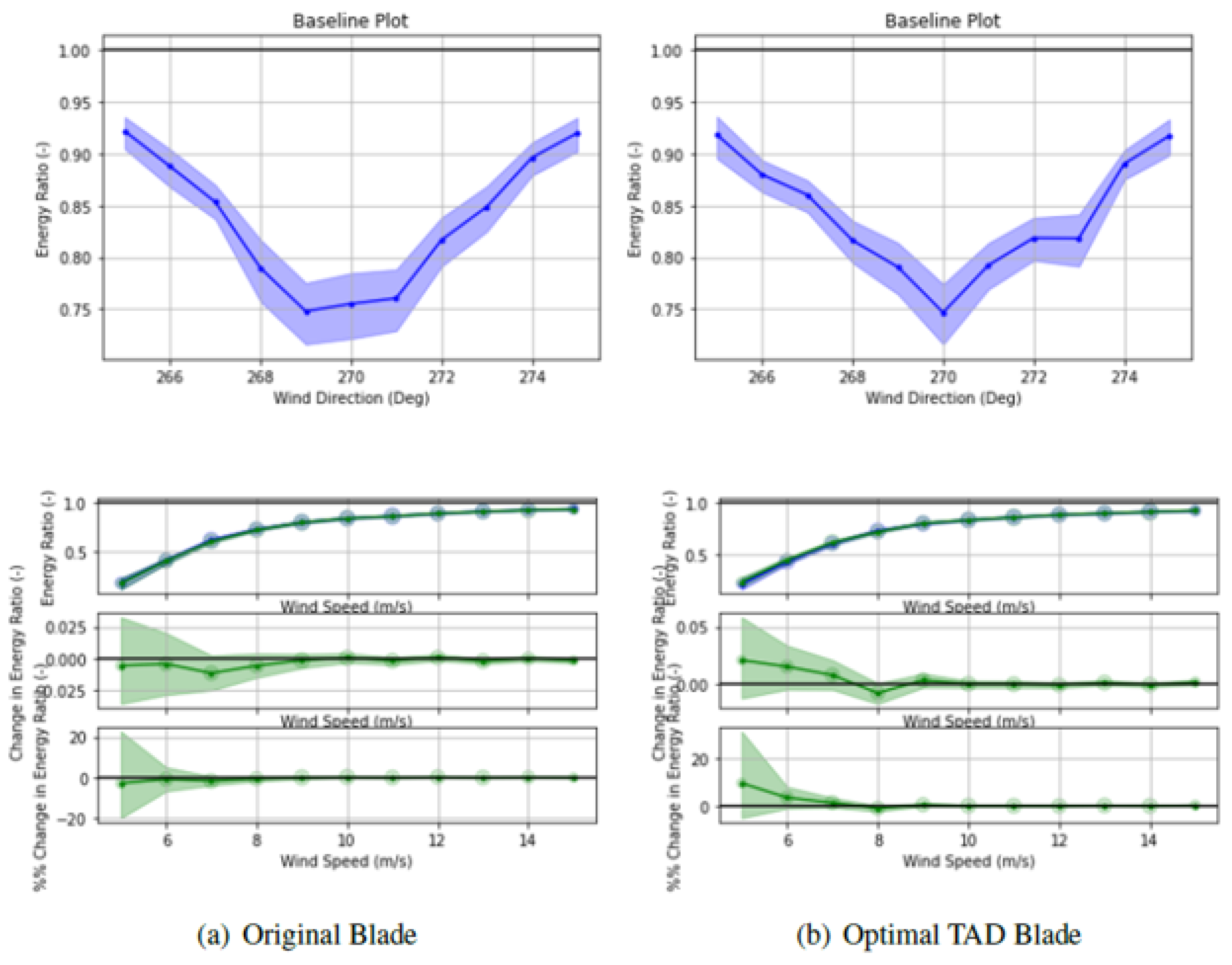
This shows that even at optimum operating speed the TAD blades show faster recovery. This indicates that there is sharp discontinuity in the wake velocity across the rotor. A smooth velocity recovery is no observed as a x-distance of 75m. This may be caused due to the transition from near to far wake. To look at this closely a comparison between the energy ratio against wind speed and direction was carried out for both TAD shapes and it can be seen in Figure 8. The TAD blade shows a higher energy ratio for a broader range of wind speeds with an exception of 270°. This indicates that a TAD blade can improve the turbine operation in region 2 with these differences becoming more significant when scaling to a larger turbine.
Figure 8.
Comparison of Wake Velocity Deficit Profile.
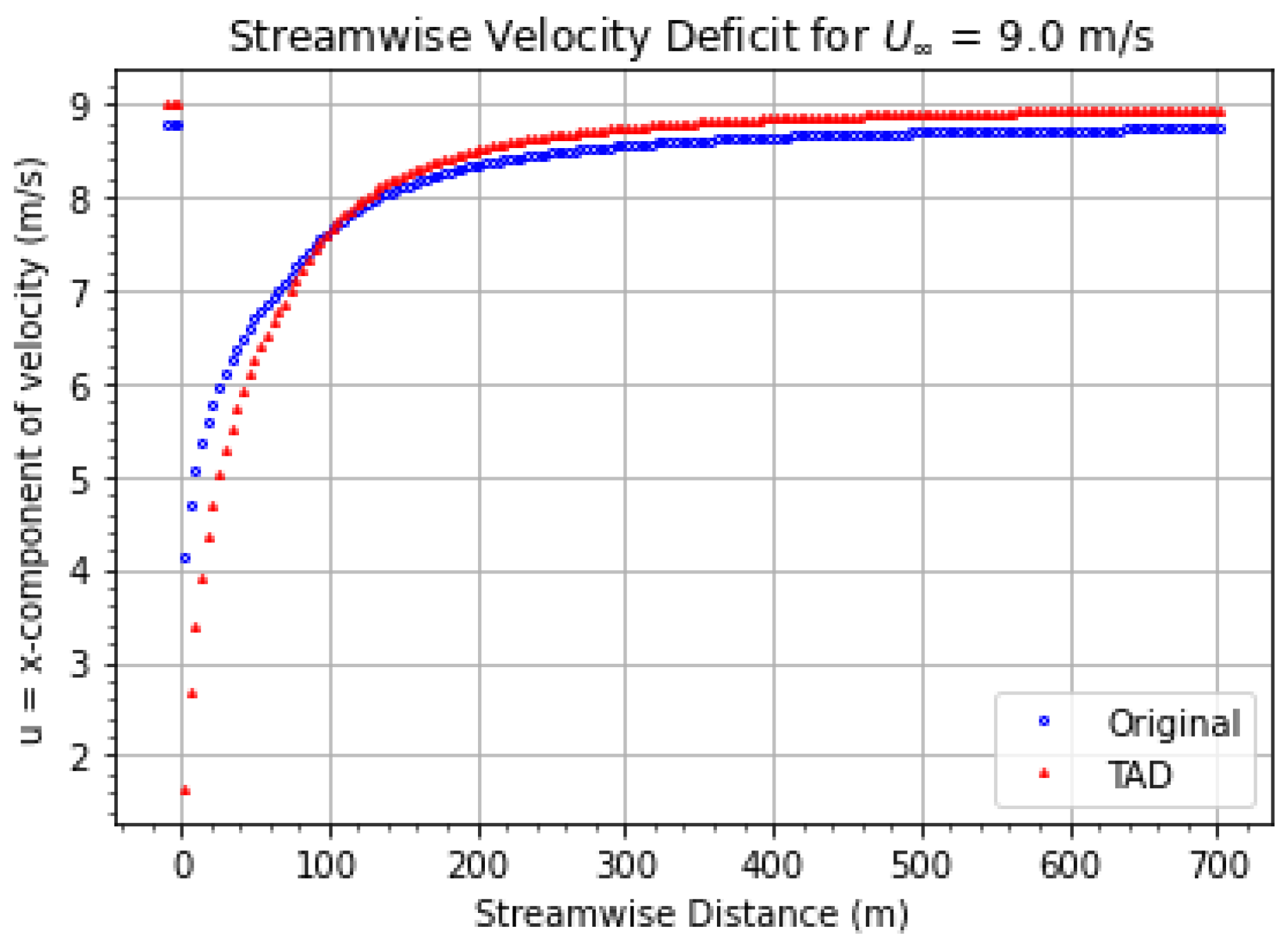
Figure 9.
Balanced Energy Ratio Against Wind Speed and Direction.
7. Conclusions
The turbine blades generate complex vortex structures form the blade tip, root and hub. Destabilization of the tip vortices due to the inflow eddies, opposite rotating vortexes stemming from the tips, the hub vortex with intense vorticity all interact with each other to generate these complex wake effects. The literature review familiarized the reader with various characteristics of wake dynamics like the immediate velocity deficit, reduction in operation lifespan due to unstable loading from TI as well as increased noise levels from these uneven loads on the downstream turbines. The scope of this projects was to get a better understanding of the wake dynamics and how the TAD blade shapes could affect these wake characteristics. FLORIS, a parametric wake modeling tool, was used to analyze steady-state wake characteristics. While transient effects due to wind speed variations are outside this scope, future work will address these phenomena. Nine TAD blade shapes were developed based on prior research, each optimized for specific wind speeds between cut-in and rated speeds. Results demonstrate that TAD blades improve wake recovery (Table 4) and reduce wake losses compared to fixed blade designs, as shown in Table 2 and Table 3. For instance, TAD #1 and TAD #9 enhance operation at cut-in and rated speeds, increasing the power coefficient by 3.83% and 3.27%, respectively. The optimal blade integrates these TAD designs, further improving efficiency across all wind speeds (Table 14 and Table 15). Validation for the optimal blade can be seen in Figure 8 showing comparable results. This study was a part of a larger body of work that looks to combine OpenFAST and FLORIS coupling, since OpenFAST could enhance the modelling capabilities especially for modelling the aero-hydro-elastic dynamics in wind turbines. This could kelpd with studying TAD shapes and their capabilities in controlling wake and a better understanding of optimal TAD shapes balancing efficiency and wake control. More work also be done using a larger scale model like the DTU 10 MW model. Validation of the work done could also be done using Fluid Structure Interactions in numerical solvers and experimental methods in wind tunnel to further the knowledge of vortex structures for TAD blades.
Author Contributions
Conceptualization, Sadeghilari and Hall.; methodology, Sadeghilari and Hall formal analysis, Sadeghilari; investigation, Sadeghilari and Hall; resources, Hall.; data curation, Hall.; writing—original draft preparation, Sadeghilari and Atre; writing—review and editing, Atre; visualization, Sadeghilari; project administration, Hall, All authors have read and agreed to the published version of the manuscript.
Data Availability Statement
The data produced or examined in this study are provided within this article.
Acknowledgments
The authors express their appreciation for the support provided by the University of North Carolina at Charlotte and the Energy Production and Infrastructure Center in facilitating this research.
Conflicts of Interest
The authors declare no conflicts of interest.
Abbreviations
The following abbreviations are used in this manuscript:
| AEP | Annual Energy Production |
| AIF | Axial Induction Factor |
| BEM | Blade ELement Momentum |
| NSE | Navier-Stokes Equation |
| Re | Reynolds Number |
| TAD | Twist Angle Distribution |
| TI | Turbulence Intensity |
| TSR | Tip Speed Ratio |
| UAE | Unsteady Aerodynamics Experiment |
References
- Administration, U.E.I.; Department, E. April 2021 Monthly Energy Review; Government Printing Office, 2021.
- Author, N.G. 2018 Wind Technologies Market Report; 2019. [CrossRef]
- Wind, I. Long-term research and development needs for wind energy for the time frame 2012 to 2030. International Energy Agency Wind, Paris, France 2013.
- Hall, J.F.; Mecklenborg, C.A.; Chen, D.; Pratap, S.B. Wind energy conversion with a variable-ratio gearbox: design and analysis. Renewable Energy 2011, 36, 1075–1080. [Google Scholar] [CrossRef]
- Burton, T.; Jenkins, N.; Sharpe, D.; Bossanyi, E. Wind Energy Handbook (John Wiley & Sons, Chicester, United Kingdom) 2011.
- Manwell, J.F.; McGowan, J.G.; Rogers, A.L. Wind energy explained: theory, design and application; John Wiley & Sons, 2010.
- Sadeghilari, K. Aerodynamic Analysis of Wake Interaction and Load Mitigation for a Wind Turbine with Active Blade Morphing Control. Master’s thesis, State University of New York at Buffalo, 2022.
- Lundquist, J.; DuVivier, K.; Kaffine, D.; Tomaszewski, J. Costs and consequences of wind turbine wake effects arising from uncoordinated wind energy development. Nature Energy 2019, 4, 26–34. [Google Scholar] [CrossRef]
- González-Longatt, F.; Wall, P.; Terzija, V. Wake effect in wind farm performance: Steady-state and dynamic behavior. Renewable Energy 2012, 39, 329–338. [Google Scholar] [CrossRef]
- Choudhry, A. Effects of Wake Interaction on Downstream Wind Turbines. Wind Engineering 2014, 38, 535–548. [Google Scholar] [CrossRef]
- Dou, B.; Guala, M.; Lei, L.; Zeng, P. Experimental investigation of the performance and wake effect of a small-scale wind turbine in a wind tunnel. Energy 2019, 166, 819–833. [Google Scholar] [CrossRef]
- Dilip, D.; Porté-Agel, F. Wind turbine wake mitigation through blade pitch offset. Energies 2017, 10, 757. [Google Scholar] [CrossRef]
- Fleming, P.; Gebraad, P.M.; Lee, S.; van Wingerden, J.W.; Johnson, K.; Churchfield, M.; Michalakes, J.; Spalart, P.; Moriarty, P. Simulation comparison of wake mitigation control strategies for a two-turbine case. Wind Energy 2015, 18, 2135–2143. [Google Scholar] [CrossRef]
- King, J.; Fleming, P.; King, R.; Martínez-Tossas, L.A.; Bay, C.J.; Mudafort, R.; Simley, E. Controls-oriented model for secondary effects of wake steering. Wind Energy Science Discussions 2020, pp. 1–22.
- MacPhee, D.W.; Beyene, A. Experimental and fluid structure interaction analysis of a morphing wind turbine rotor. Energy 2015, 90, 1055–1065. [Google Scholar] [CrossRef]
- Wang, W.; Caro, S.; Bennis, F.; Salinas Mejia, O.R. A simplified morphing blade for horizontal axis wind turbines. Journal of solar energy engineering 2014, 136. [Google Scholar] [CrossRef]
- Barbarino, S.; Bilgen, O.; Ajaj, R.M.; Friswell, M.I.; Inman, D.J. A review of morphing aircraft. Journal of intelligent material systems and structures 2011, 22, 823–877. [Google Scholar] [CrossRef]
- Weisshaar, T.A. Morphing aircraft systems: historical perspectives and future challenges. Journal of aircraft 2013, 50, 337–353. [Google Scholar] [CrossRef]
- Ponta, F.L.; Otero, A.D.; Rajan, A.; Lago, L.I. The adaptive-blade concept in wind-power applications. Energy for Sustainable Development 2014, 22, 3–12. [Google Scholar] [CrossRef]
- Rauleder, J.; van der Wall, B.G.; Abdelmoula, A.; Komp, D.; Kumar, S.; Ondra, V.; Titurus, B.; Woods, B.K. Aerodynamic performance of morphing blades and rotor systems. In Proceedings of the AHS International 74th Annual Forum & Technology Display, 2018, p. 1.
- Sofla, A.; Meguid, S.; Tan, K.; Yeo, W. Shape morphing of aircraft wing: Status and challenges. Materials & Design 2010, 31, 1284–1292. [Google Scholar] [CrossRef]
- Hattalli, V.L.; Srivatsa, S.R. Wing Morphing to Improve Control Performance of an Aircraft-An Overview and a Case Study. Materials Today: Proceedings 2018, 5, 21442–21451. [Google Scholar] [CrossRef]
- Hassanzadeh, A.; Hassanabad, A.H.; Dadvand, A. Aerodynamic shape optimization and analysis of small wind turbine blades employing the Viterna approach for post-stall region. Alexandria Engineering Journal 2016, 55, 2035–2043. [Google Scholar] [CrossRef]
- Loth, E.; Selig, M.; Moriarty, P. Morphing segmented wind turbine concept. In Proceedings of the 28th AIAA Applied Aerodynamics Conference, 2010, p. 4400.
- Gili, P.; Frulla, G. A variable twist blade concept for more effective wind generation: design and realization. Smart Science 2016, 4, 78–86. [Google Scholar] [CrossRef]
- Daynes, S.; Weaver, P. Design and testing of a deformable wind turbine blade control surface. Smart Materials and Structures 2012, 21, 105019. [Google Scholar] [CrossRef]
- Khakpour Nejadkhaki, H.; Hall, J.F. A Design Methodology for a Flexible Wind Turbine Blade With an Actively Variable Twist Distribution to Increase Region 2 Efficiency. In Proceedings of the International Design Engineering Technical Conferences and Computers and Information in Engineering Conference. American Society of Mechanical Engineers, 2017, Vol. 58127, p. V02AT03A025.
- Nejadkhaki, H.K.; Hall, J.F. Modeling and Design Method for an Adaptive Wind Turbine Blade With Out-of-Plane Twist. Journal of Solar Energy Engineering 2018, 140. [Google Scholar] [CrossRef]
- Nejadkhaki, H.K.; Hall, J.F. Integrative Control and Design Framework for an Actively Variable Twist Wind Turbine Blade to Increase Efficiency. In Proceedings of the International Design Engineering Technical Conferences and Computers and Information in Engineering Conference. American Society of Mechanical Engineers, 2018, Vol. 51753, p. V02AT03A004.
- Khakpour Nejadkhaki, H.; Hall, J.F. Control Framework and Integrative Design Method for an Adaptive Wind Turbine Blade. Journal of Dynamic Systems, Measurement, and Control 2020, 142, 101001. [Google Scholar] [CrossRef]
- Blevins, R.D. Applied fluid dynamics handbook. vnr 1984. [Google Scholar]
- Cardell, G.S. Flow past a circular cylinder with a permeable wake splitter plate. PhD thesis, California Institute of Technology, 1993.
- Panton, R.L. Incompressible flow; John Wiley & Sons, 2013.
- Sanderse, B. Aerodynamics of wind turbine wakes Literature review 2009.
- Felli, M.; Falchi, M. Propeller wake evolution mechanisms in oblique flow conditions. Journal of Fluid Mechanics 2018, 845, 520. [Google Scholar] [CrossRef]
- Vermeer, L.; Sørensen, J.N.; Crespo, A. Wind turbine wake aerodynamics. Progress in aerospace sciences 2003, 39, 467–510. [Google Scholar] [CrossRef]
- Ozbay, A. Experimental investigations on the wake interferences of multiple wind turbines 2012.
- Porté-Agel, F.; Bastankhah, M.; Shamsoddin, S. Wind-turbine and wind-farm flows: a review. Boundary-Layer Meteorology 2020, 174, 1–59. [Google Scholar] [CrossRef] [PubMed]
- NREL. FLORIS Wake Modeling Utility - FLORIS 2.2.0 Documentation, 2020.
- Ramírex Castillo, S.A. Engineering models enhancement for wind farm wake simulation and optimization 2019.
- Raach, S.; Campagnolo, F.; Ramamurthy, B.K.; Kern, S.; Boersma, S.; Doekemeijer, B.; van Wingerden, J.W.; Knudsen, T.; Kanev, S.; Aparicio-Sanchez, M.; et al. Classification of control-oriented models for wind farm control applications, 2019. [CrossRef]
- Jensen, N.O. A note on wind generator interaction 1983.
- Bay, C.; King, J.; Fleming, P.; Martínez-Tossas, L.; Mudafort, R.; Simley, E.; Lawson, M. FLORIS: A Brief Tutorial, 2019.
- Annoni, J.; Fleming, P.; Scholbrock, A.K.; Roadman, J.M.; Dana, S.; Adcock, C.; Porte-Agel, F.; Raach, S.; Haizmann, F.; Schlipf, D. Analysis of control-oriented wake modeling tools using lidar field results. Wind Energy Science (Online) 2018, 3. [Google Scholar] [CrossRef]
- Gebraad, P.M.; Teeuwisse, F.; van Wingerden, J.W.; Fleming, P.A.; Ruben, S.D.; Marden, J.R.; Pao, L.Y. A data-driven model for wind plant power optimization by yaw control. In Proceedings of the 2014 American Control Conference. IEEE, 2014, pp. 3128–3134.
- Jiménez, Á.; Crespo, A.; Migoya, E. Application of a LES technique to characterize the wake deflection of a wind turbine in yaw. Wind energy 2010, 13, 559–572. [Google Scholar] [CrossRef]
- Bastankhah, M.; Porté-Agel, F. Experimental and theoretical study of wind turbine wakes in yawed conditions. Journal of Fluid Mechanics 2016, 806, 506. [Google Scholar] [CrossRef]
- Fleming, P.; King, J.; Bay, C.J.; Simley, E.; Mudafort, R.; Hamilton, N.; Farrell, A.; Martinez-Tossas, L. Overview of FLORIS updates. In Proceedings of the Journal of Physics: Conference Series. IOP Publishing, 2020, Vol. 1618, p. 022028.
- Martínez-Tossas, L.A.; Annoni, J.; Fleming, P.A.; Churchfield, M.J. The aerodynamics of the curled wake: A simplified model in view of flow control. Wind Energy Science (Online) 2019, 4. [Google Scholar] [CrossRef]
- Neiva, A.; Guedes, V.; Massa, C.; de Freitas, D. A review of wind turbine wake models for microscale wind park simulation. ABCM International Congress of Mechanical Engineering, 2019.
- Niayifar, A.; Porté-Agel, F. A new analytical model for wind farm power prediction. In Proceedings of the Journal of physics: conference series. IOP Publishing, 2015, Vol. 625, p. 012039. [CrossRef]
- Farrell, A.; King, J.; Draxl, C.; Mudafort, R.; Hamilton, N.; Bay, C.J.; Fleming, P.; Simley, E. Design and analysis of a spatially heterogeneous wake. Wind Energy Science Discussions 2020, pp. 1–25.
- Niayifar, A.; Porté-Agel, F. Analytical modeling of wind farms: A new approach for power prediction. Energies 2016, 9, 741. [Google Scholar] [CrossRef]
- Crespo, A.; Herna, J.; et al. Turbulence characteristics in wind-turbine wakes. Journal of wind engineering and industrial aerodynamics 1996, 61, 71–85. [Google Scholar] [CrossRef]
- Doekemeijer, B.; Bossanyi, E.; Kanev, S.; Bot, E.; Elorza, I.; Campagnolo, F.; Fortes-Plaza, A.; Schreiber, J.; Eguinoa-Erdozain, I.; Gomez-Iradi, S.; et al. Description of the reference and the control-oriented wind farm models, 2018. [CrossRef]
- NREL. FLORIS. Version 2.2.0, 2020.
- Doekemeijer, B.; Storm, R.; Schreiber, J.; daanvanderhoek. TUDelft-DataDrivenControl/FLORISSE_M: Stable version from 2018-2019, 2021. [CrossRef]
- Gebraad, P.; Thomas, J.J.; Ning, A.; Fleming, P.; Dykes, K. Maximization of the annual energy production of wind power plants by optimization of layout and yaw-based wake control. Wind Energy 2017, 20, 97–107. [Google Scholar] [CrossRef]
- Cioffi, A.; Muscari, C.; Schito, P.; Zasso, A. A Steady-State Wind Farm Wake Model Implemented in OpenFAST. Energies 2020, 13, 6158. [Google Scholar] [CrossRef]
- Thomas, J.J.; Gebraad, P.M.; Ning, A. Improving the FLORIS wind plant model for compatibility with gradient-based optimization. Wind Engineering 2017, 41, 313–329. [Google Scholar] [CrossRef]
- TU Delft DCSC Data Driven Control Group Revision. FLORISSE M Documentation, 2019.
- NREL. OpenFAST Documentation Release v2.5.0, 2021.
- Churchfield, M.; Lee, S.; Moriarty, P. Overview of the simulator for wind farm application (SOWFA). National Renewable Energy Laboratory 2012. [Google Scholar]
- Drela, M.; Youngren, H. XFOIL 6.94 user guide, 2001.
- Marten, D.; Wendler, J. Qblade guidelines. Ver. 0.6, Technical University of (TU Berlin), Berlin, Germany 2013.
- Hand, M.; Simms, D.; Fingersh, L.; Jager, D.; Cotrell, J.; Schreck, S.; Larwood, S. Unsteady aerodynamics experiment phase VI: wind tunnel test configurations and available data campaigns. Technical report, National Renewable Energy Lab., Golden, CO.(US), 2001.
- Moriarty, P.J.; Hansen, A.C. AeroDyn theory manual. Technical report, National Renewable Energy Lab., Golden, CO (US), 2005.
- Hansen, M. Aerodynamics of wind turbines; Routledge, 2015.
- Fleming, P.; King, J.; Dykes, K.; Simley, E.; Roadman, J.; Scholbrock, A.; Murphy, P.; Lundquist, J.K.; Moriarty, P.; Fleming, K.; et al. Initial results from a field campaign of wake steering applied at a commercial wind farm–Part 1. Wind Energy Science 2019, 4, 273–285. [Google Scholar] [CrossRef]
- Fleming, P.; King, J.; Simley, E.; Roadman, J.; Scholbrock, A.; Murphy, P.; Lundquist, J.K.; Moriarty, P.; Fleming, K.; Dam, J.v.; et al. Continued results from a field campaign of wake steering applied at a commercial wind farm–Part 2. Wind Energy Science 2020, 5, 945–958. [Google Scholar] [CrossRef]
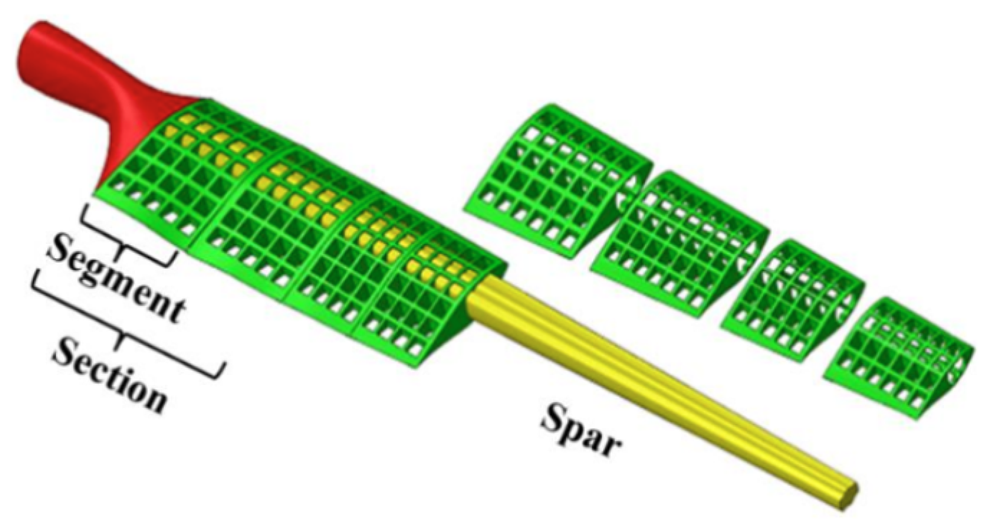
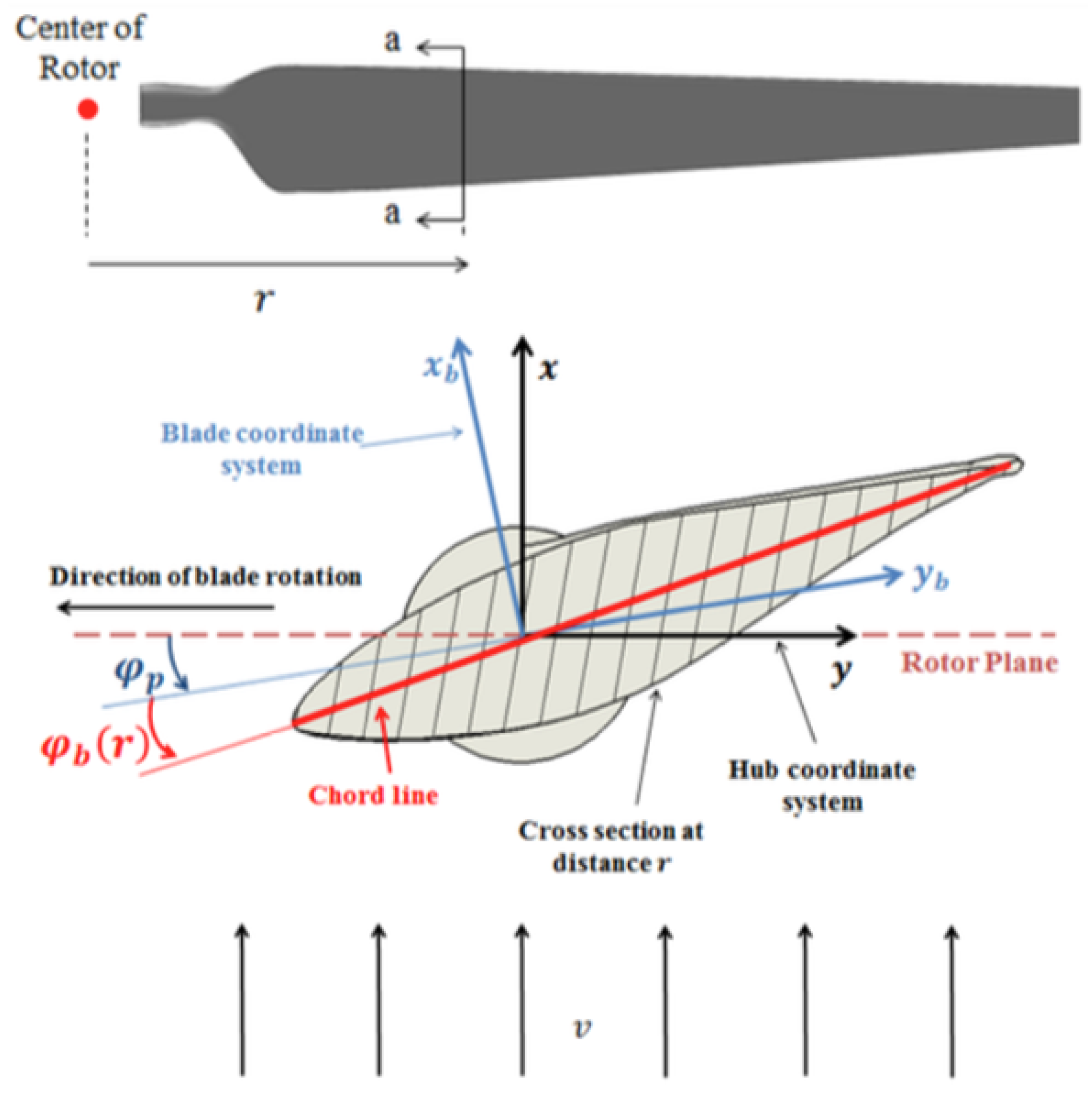
Figure 4.
Framework for the Active Blade Twist Angle Distribution.
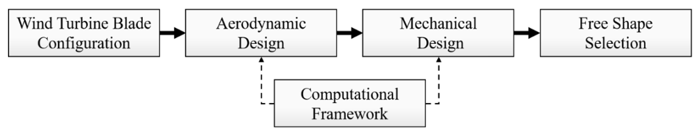
Figure 5.
1x3 Wind Farm Layout.
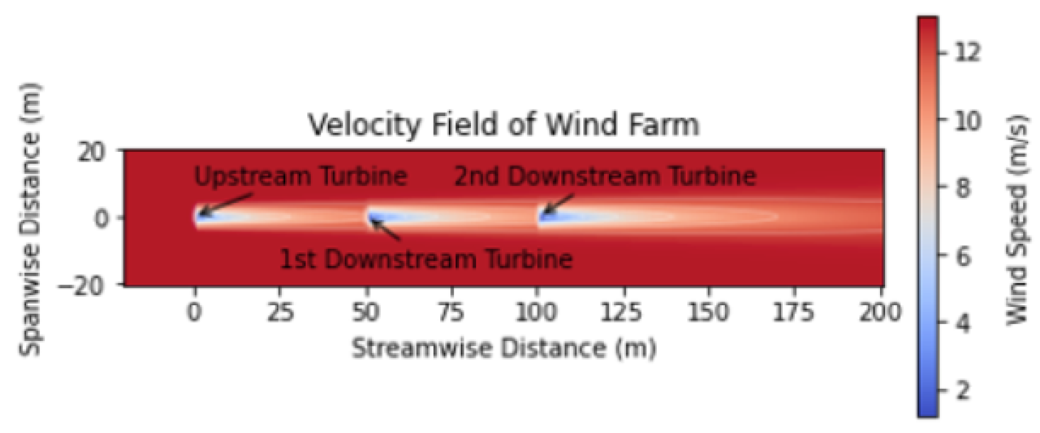
Figure 6.
2x1 Wind Farm Layout.
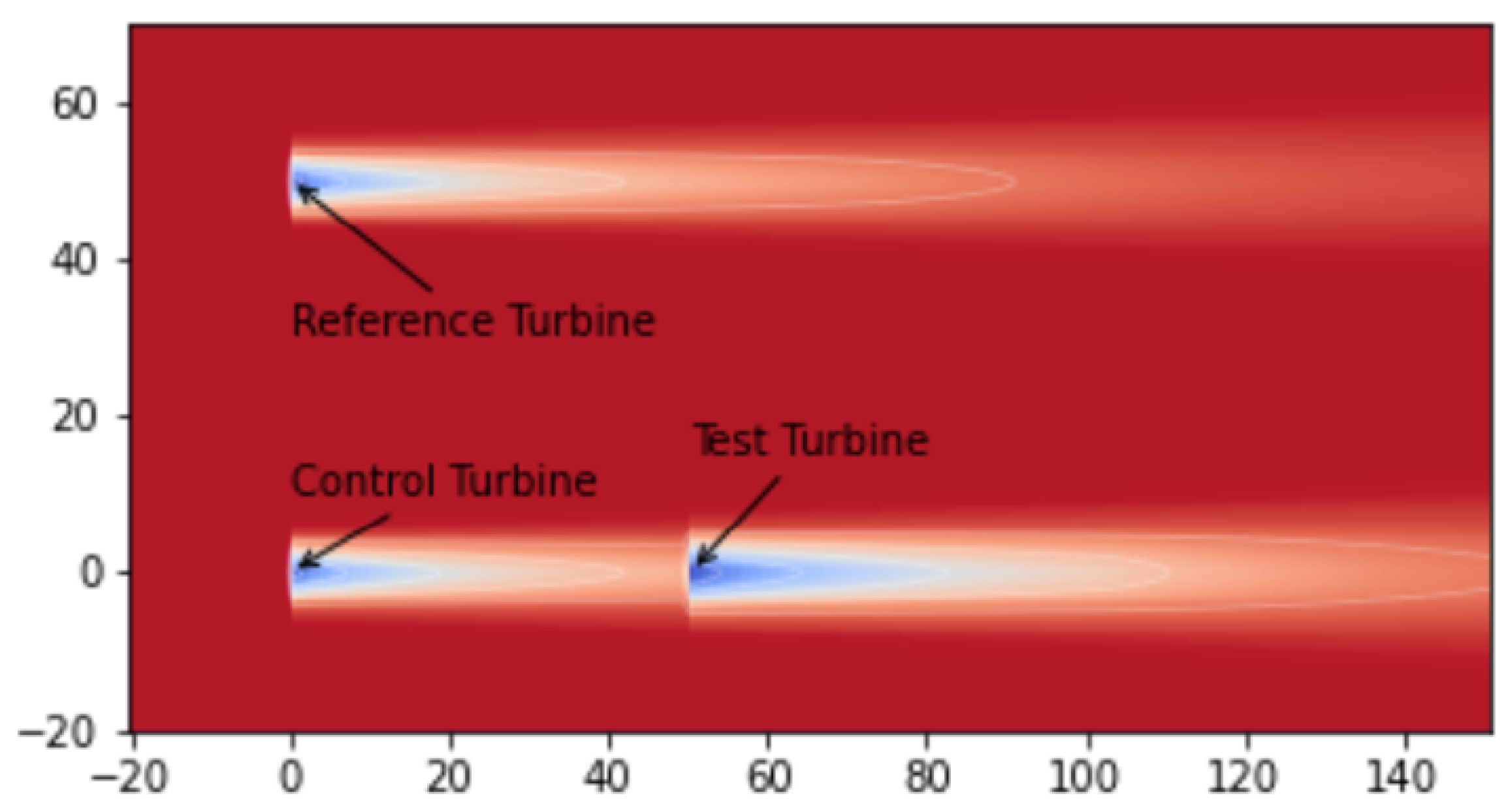
Figure 7.
Minimum Wake Loss Blade.
Table 4.
Distances for Full Velocity Recovery.
| [m/s] | 5 | 6 | 7 | 8 | 9 | 10 | 11 | 12 | 13 |
| Original | 1994 | 1971 | 1888 | 1804 | 1735 | 1676 | 1626 | 1575 | 1527 |
| TAD #1 | 1994 | 1997 | 1903 | 1814 | 1751 | 1692 | 1634 | 1599 | 1558 |
| TAD #2 | 1994 | 1993 | 1903 | 1812 | 1738 | 1684 | 1637 | 1594 | 1556 |
| TAD #3 | 1994 | 1983 | 1901 | 1812 | 1737 | 1667 | 1601 | 1576 | 1535 |
| TAD #4 | 1994 | 1977 | 1898 | 1843 | 1742 | 1677 | 1615 | 1553 | 1503 |
| TAD #5 | 1994 | 1974 | 1895 | 1810 | 1746 | 1682 | 1628 | 1577 | 1532 |
| TAD #6 | 1994 | 1967 | 1888 | 1806 | 1739 | 1681 | 1621 | 1577 | 1533 |
| TAD #7 | 1994 | 1952 | 1875 | 1795 | 1726 | 1671 | 1619 | 1571 | 1529 |
| TAD #8 | 1994 | 1943 | 1863 | 1788 | 1722 | 1663 | 1615 | 1573 | 1534 |
| TAD #9 | 1994 | 1936 | 1860 | 1783 | 1718 | 1660 | 1610 | 1570 | 1531 |
Table 5.
Percentage Change in Recovered Distances.
| [m/s] | 5 | 6 | 7 | 8 | 9 | 10 | 11 | 12 | 13 |
| TAD #7 | 0.00% | -0.96% | -0.69% | -0.50% | -0.52% | -0.30% | -0.43% | -0.25% | 0.13% |
| TAD #8 | 0.00% | -1.42% | -1.32% | -0.89% | -0.75% | -0.78% | -0.68% | -0.13% | 0.46% |
| TAD #9 | 0.00% | -1.78% | -1.48% | -1.16% | -0.98% | -0.95% | -0.98% | -0.32% | 0.26% |
Table 6.
Upstream Turbine Power Output in kW.
| [m/s] | Original | TAD #1 | TAD #2 | TAD #3 | TAD #4 | TAD #5 | TAD #6 | TAD #7 | TAD #8 | TAD #9 |
| 5 | 2.68 | 2.79 | 2.77 | 2.75 | 2.71 | 2.68 | 2.66 | 2.61 | 2.55 | 2.54 |
| 6 | 5.03 | 5.05 | 5.09 | 5.07 | 5.02 | 5.02 | 5.00 | 4.97 | 4.90 | 4.89 |
| 7 | 7.20 | 7.15 | 7.23 | 7.27 | 7.22 | 7.18 | 7.17 | 7.14 | 7.07 | 7.06 |
| 8 | 9.18 | 8.93 | 9.10 | 9.20 | 9.30 | 9.18 | 9.17 | 9.14 | 9.06 | 9.05 |
| 9 | 11.10 | 10.61 | 10.73 | 11.00 | 11.10 | 11.11 | 11.11 | 11.09 | 11.03 | 11.01 |
| 10 | 12.99 | 12.26 | 12.48 | 12.66 | 12.92 | 12.98 | 13.06 | 13.05 | 13.01 | 12.98 |
| 11 | 14.88 | 13.96 | 14.27 | 14.19 | 14.71 | 14.79 | 14.92 | 15.04 | 15.02 | |
| 12 | 16.76 | 15.70 | 16.18 | 15.81 | 16.38 | 16.65 | 16.74 | 17.00 | 17.08 | 17.06 |
| 13 | 17.96 | 16.89 | 17.44 | 16.95 | 17.44 | 17.86 | 17.97 | 18.27 | 18.43 | 18.44 |
Table 7.
Downstream Turbine Power Output in kW.
| [m/s] | Original | TAD #1 | TAD #2 | TAD #3 | TAD #4 | TAD #5 | TAD #6 | TAD #7 | TAD #8 | TAD #9 |
| 5 | -1.99 | -1.72 | -1.85 | -1.85 | -1.87 | -1.98 | -2.01 | -2.07 | -2.14 | -2.13 |
| 6 | -0.50 | -0.35 | -0.43 | -0.41 | -0.43 | -0.50 | -0.51 | -0.53 | -0.57 | -0.54 |
| 7 | 2.17 | 2.22 | 2.18 | 2.18 | 2.16 | 2.14 | 2.14 | 2.17 | 2.16 | 2.17 |
| 8 | 4.87 | 4.85 | 4.90 | 4.88 | 4.69 | 4.84 | 4.83 | 4.85 | 4.81 | 4.82 |
| 9 | 7.25 | 7.14 | 7.27 | 7.31 | 7.25 | 7.20 | 7.21 | 7.23 | 7.17 | 7.18 |
| 10 | 9.38 | 9.06 | 9.25 | 9.42 | 9.49 | 9.36 | 9.36 | 9.36 | 9.32 | 9.31 |
| 11 | 11.43 | 10.84 | 10.97 | 11.35 | 11.42 | 11.41 | 11.44 | 11.43 | 11.39 | 11.38 |
| 12 | 13.44 | 12.57 | 12.82 | 13.01 | 13.40 | 13.38 | 13.48 | 13.51 | 13.47 | 13.45 |
| 13 | 15.46 | 14.37 | 14.72 | 14.63 | 15.28 | 15.32 | 15.43 | 15.61 | 15.60 | 15.58 |
Table 8.
2nd Downstream Turbine Power Output in kW.
| [m/s] | Original | TAD #1 | TAD #2 | TAD #3 | TAD #4 | TAD #5 | TAD #6 | TAD #7 | TAD #8 | TAD #9 |
| 5 | -0.94 | -0.70 | -0.81 | -0.81 | -0.84 | -0.93 | -0.96 | -1.02 | -1.08 | -1.08 |
| 6 | 0.13 | 0.36 | 0.28 | 0.26 | 0.22 | 0.15 | 0.11 | 0.03 | -0.04 | -0.05 |
| 7 | 1.42 | 1.58 | 1.53 | 1.52 | 1.48 | 1.43 | 1.39 | 1.33 | 1.26 | 1.25 |
| 8 | 2.88 | 2.91 | 2.91 | 2.92 | 2.91 | 2.88 | 2.87 | 2.87 | 2.83 | 2.84 |
| 9 | 5.25 | 5.14 | 5.20 | 5.20 | 5.16 | 5.17 | 5.20 | 5.28 | 5.29 | 5.30 |
| 10 | 7.92 | 7.74 | 7.88 | 7.96 | 7.81 | 7.87 | 7.88 | 7.91 | 7.88 | 7.90 |
| 11 | 10.19 | 9.74 | 9.93 | 10.18 | 10.24 | 10.15 | 10.17 | 10.20 | 10.15 | 10.16 |
| 12 | 12.34 | 11.60 | 11.80 | 12.13 | 12.31 | 12.31 | 12.36 | 12.38 | 12.36 | 12.35 |
| 13 | 14.45 | 13.46 | 13.74 | 13.86 | 14.35 | 14.32 | 14.47 | 14.56 | 14.54 | 14.53 |
Table 9.
Percent Change in the Upstream Turbine Power Generation.
| [m/s] | 5 | 6 | 7 | 8 | 9 | 10 | 11 | 12 | 13 |
| TAD #3 | 2.58% | 0.75% | 0.99% | 0.21% | -0.87% | -2.58% | -4.66% | -5.65% | -5.61% |
| TAD #6 | -1.02% | -0.67% | -0.39% | -0.04% | 0.11% | 0.51% | 0.25% | -0.13% | 0.10% |
| TAD #7 | -2.58% | -1.26% | -0.80% | -0.45% | -0.07% | 0.41% | 1.03% | 1.44% | 1.76% |
| TAD #8 | -5.06% | -2.61% | -1.76% | -1.22% | -0.61% | 0.12% | 0.92% | 1.92% | 2.64% |
Table 10.
Percent Change in the 1st Downstream Turbine Power Generation.
| [m/s] | 5 | 6 | 7 | 8 | 9 | 10 | 11 | 12 | 13 |
| TAD #2 | 7.23% | 13.50% | 0.51% | 0.42% | 0.32% | -1.40% | -4.01% | -4.64% | -4.78% |
| TAD #3 | 7.26% | 17.61% | 0.53% | 0.07% | 0.82% | 0.42% | -0.65% | -3.26% | -5.38% |
| TAD #6 | -0.64% | -1.40% | -1.13% | -0.91% | -0.58% | -0.22% | 0.11% | 0.27% | -0.20% |
| TAD #7 | -4.01% | -5.06% | -0.08% | -0.56% | -0.33% | -0.22% | -0.02% | 0.49% | 0.95% |
| TAD #8 | -7.23% | -12.76% | -0.34% | -1.31% | -1.06% | -0.64% | -0.37% | 0.16% | 0.88% |
Table 11.
Percent Change in the 2nd Downstream Turbine Power Generation.
| [m/s] | 5 | 6 | 7 | 8 | 9 | 10 | 11 | 12 | 13 |
| TAD #1 | 25.19% | 175.35% | 11.56% | 1.04% | -2.09% | -2.25% | -4.40% | -6.02% | -6.88% |
| TAD #3 | 13.58% | 95.81% | 7.10% | 1.13% | -0.77% | 0.53% | -0.09% | -1.73% | -4.11% |
| TAD #4 | 10.83% | 67.03% | 4.43% | 1.00% | -1.70% | -1.39% | 0.49% | -0.26% | -0.69% |
| TAD #6 | -1.71% | -18.39% | -1.66% | -0.53% | -0.79% | -0.50% | -0.17% | 0.16% | 0.14% |
| TAD #7 | -8.24% | -74.15% | -5.86% | -0.59% | 0.63% | -0.12% | 0.04% | 0.30% | 0.77% |
| TAD #8 | -15.12% | -132.05% | -11.24% | -2.01% | 0.80% | -0.46% | -0.37% | 0.15% | 0.61% |
Table 12.
Wake loss percentage.
 |
Table 13.
Summary of Change in Wake Loss Percent.
| TAD #1 | TAD #2 | TAD #3 | TAD #4 | TAD #5 | TAD #6 | TAD #7 | TAD #8 | TAD #9 | |
| max In | 5.7% | 7.7% | 8.9% | 6.2% | 7.6% | 7.3% | 7.1% | 4.8% | 6.7% |
| max Red | -2.8% | -5.9% | -5.0% | -3.2% | -2.5% | -1.1% | -9.9% | -4.8% | -4.7% |
| 8.4% | 13.6% | 13.9% | 9.4% | 10.1% | 8.3% | 17.0% | 9.6% | 11.4% | |
| 2.9% | 1.8% | 3.9% | 3.1% | 5.0% | 6.2% | -2.8% | 0.1% | 2.0% |
Table 14.
Power coefficients for the Original and Optimum TAD.
| [m/s] | 5 | 6 | 7 | 8 | 9 | 10 | 11 | 12 | 13 |
| 0.447 | 0.484 | 0.435 | 0.370 | 0.314 | 0.268 | 0.231 | 0.200 | 0.174 | |
| 0.464 | 0.489 | 0.440 | 0.377 | 0.315 | 0.270 | 0.233 | 0.204 | 0.180 | |
| ln [%] | 3.83 | 1.05 | 1.13 | 1.76 | 0.13 | 0.63 | 1.08 | 1.90 | 3.27 |
Table 15.
Thrust coefficients for the Original and Optimum TAD.
| [m/s] | 5 | 6 | 7 | 8 | 9 | 10 | 11 | 12 | 13 |
| 0.817 | 0.793 | 0.617 | 0.490 | 0.401 | 0.336 | 0.286 | 0.245 | 0.212 | |
| 0.851 | 0.811 | 0.626 | 0.512 | 0.407 | 0.338 | 0.286 | 0.247 | 0.215 | |
| ln [%] | 4.11 | 2.33 | 1.36 | 4.45 | 1.30 | 0.62 | 0.11 | 0.69 | 1.46 |
Disclaimer/Publisher’s Note: The statements, opinions and data contained in all publications are solely those of the individual author(s) and contributor(s) and not of MDPI and/or the editor(s). MDPI and/or the editor(s) disclaim responsibility for any injury to people or property resulting from any ideas, methods, instructions or products referred to in the content. |
© 2025 by the authors. Licensee MDPI, Basel, Switzerland. This article is an open access article distributed under the terms and conditions of the Creative Commons Attribution (CC BY) license (http://creativecommons.org/licenses/by/4.0/).
Copyright: This open access article is published under a Creative Commons CC BY 4.0 license, which permit the free download, distribution, and reuse, provided that the author and preprint are cited in any reuse.


