Data Mining and Machine Learning Approaches for Analyzing Drug-Related Overdose Patterns and Risk Factors

1. Introduction

The drug overdose epidemic is an enormous public health hazard worldwide that requires sophisticated analytical approaches to discover and address the epidemic. Among the wide variety of drugs, fentanyl and fentanyl analogs, typically mixed with drugs like xylazine, have become central to deadly overdoses due to their high potency and unstable effects. Detection of which population segments are most vulnerable is central to the development of targeted prevention and intervention strategies. Further, detection of drug consumption patterns, geographic displacement patterns, and trafficking networks can enable more informed understanding of the dynamics of drug overdose incidents. For these purposes, data mining and machine learning techniques have been found to be extremely useful in discovering meaningful insights from large, complex data sets [1].

Through the use of clustering models such as KMeans and HDBSCAN, researchers are able to categorize populations and detect latent patterns that may not be revealed by regular statistical methods. Similarly, predictive models such as Random Forest, Support Vector Machine, and K-Nearest Neighbors enhance substance involvement prediction and risk factors forecasting to be more precise and possible for improved public health targeting. Besides, anomaly detection methods can identify suspicious patterns of movement for drug purchase and overdose that are valuable information to law enforcers and healthcare clinicians. This paper analyzes these analytical techniques applied to drug overdose death datasets in an attempt to define high-risk populations, local outliers, and hidden patterns. The goal is to facilitate the creation of effective, evidence-based harm reduction interventions and policies that can reverse the tide of overdose fatalities[2,3].

The increasing trend in drug overdose-related accidental fatalities is a critical public health and law enforcement issue that needs sophisticated analytic methods to further contextualize and address the underlying causes. One of the steps in this process involves the application of such clustering algorithms as KMeans and HDBSCAN to identify population segments at risk and expose overdoses patterns. By breaking people up into groups on the basis of such criteria as age, drug involvement, and geography, such methods can uncover hidden patterns that are normally below the threshold for conventional statistical scrutiny. Having a sense of reason and impact for these overdoses—e.g., the potency of drugs like fentanyl, use of drugs in combination, socio-economics, and obliviousness—facilitates direction for intervention activity. Different demographic segments are exposed to various risks; for instance, younger segments are more likely to use drugs, whereas elderly individuals can be affected by prescription errors. In the absence of proper segmentation, efforts to prevent overdose deaths are blanket and futile, and fentanyl and other drugs continue to claim lives. Therefore, this clustering approach is meant to inform public health interventions, including targeted awareness campaigns and harm reduction efforts. A comparison of how well algorithms like KMeans and HDBSCAN perform will identify the action to be taken by policymakers and healthcare professionals in an effort to stop drug-related deaths[4,5,6,7].

A second urgent issue is the unusual geographic displacement of victims in most drug-related fatalities, wherein they are frequently discovered from their homes or point of first injury far away. This issue indicates intricate dynamics between drug trafficking routes, accessibility, response delays in emergency, and socioeconomic vulnerabilities. With the data in 'Accidental_Drug_Related_Deaths.csv,' this study attempts to find spatial irregularities—e.g., when individuals pass away more than 150 km from the injury location or travel more than 4,200 km before their death—that may reflect drug tourism, organized selling networks, or systemic relocation activity. These locational displacements can be the consequence of non-reported homelessness, late medical intervention, or self-initiated journey to purchase drugs, all difficult to intervene on. Ignoring these patterns of movement risks overlooking vital factors contributing to overdose fatalities, thereby obliterating successful harm reduction strategies. By employing anomaly detection techniques, this research seeks to uncover hidden patterns of movement so policymakers, healthcare workers, and law enforcement can develop targeted interventions, optimize emergency response protocols, and more effectively distribute resources. Lastly, understanding these spatial dynamics will improve public health interventions and reduce overdose deaths related to these hidden mobility patterns [8,9,10].

2. Literature Review

The opioid crisis, particularly fentanyl, fentanyl analogues, and xylazine, has escalated in the past few years and accounted for a significant rise in fatal overdoses. It is critical to identify high-risk populations and to clarify the underlying trends of drug overdose mortality to create effective public health interventions and harm reduction strategies.

Recent literature indicates that the lethality of fentanyl and its analogs is heightened when combined with xylazine, a veterinary sedative non-human use approved. Deaths by overdose using these drugs have escalated, and some age groups have been disproportionately affected. Studies indicate that younger individuals may be at greater risk through experimentation and naivety, whereas older individuals are at higher risk due to chronic pain management and prescription misuse. The Centers for Disease Control and Prevention (CDC) states that individuals aged 25–54 are most commonly behind synthetic opioid overdose deaths, yet there is also an alarming surge among adolescents and young adults [11].

Its co-administration with fentanyl has been associated with an increased risk of fatal overdose because xylazine is not an opioid and will not respond to naloxone, which is the optimal opioid overdose antidote. It becomes harder for emergency responders and adds risk across all ages but most notably among individuals who may be unaware that illicit drugs might contain xylazine. Traditional statistical methods may be unsensitive to fine-grained patterns in drug overdose death. Data mining and machine learning methods, such as KMeans and HDBSCAN clustering, enable researchers to cluster populations by age, drug use, and other factors and detect hidden risk groups. For example, the KMeans method has been effectively used to detect high-risk subpopulations for overdose, which revealed that poly-drug use and socioeconomic status are significant influencers of overdose death [12].

HDBSCAN, a density-based clustering algorithm, has the advantage of identifying clusters of varying shapes and densities, which is of particular interest for the identification of demographic groups at higher risk that are not identified by partition-based algorithms like KMeans. Such algorithms enable the development of targeted interventions, such as focused awareness campaigns and harm reduction strategies, that can be targeted to the most vulnerable groups. Geographic displacement—where the overdose victims are found far from home or the location of initial injury—has emerged as a central phenomenon of drug-related fatalities. Research suggests that this displacement is due to drug tourism, trafficking routes, homelessness, and the delayed nature of emergencies. Anomaly detection techniques on spatial data have discovered the mobility patterns involved in drug procurement and overdose, which are crucial to understand the spread of the opioid epidemic and deploy resources effectively [13,14].

Instances of subjects traveling long distances prior to fatal overdose can suggest either organized distribution chains or voids in health care services within local areas. Failure to pay attention to these geographic patterns can lead to inefficacious harm reduction policy and missed potential for targeted intervention.

Machine learning models—Random Forest, Support Vector Machine (SVM), and K-Nearest Neighbors (KNN)—have been helpful in classifying and predicting cases of drug overdose. Feature selection, missing value imputation, encoding categorical variables, and standardization of numerical features are necessary preprocessing steps for model performance. These models allow for the determination of high-risk age groups and the prediction of overdose risk, enabling proactive public health responses [15,16].

The use of advanced data mining and machine learning algorithms in the study of drug-related deaths provides a deeper understanding of the opioid crisis. By identifying high-risk age groups, uncovering hidden demographic clusters, and charting geographic displacement patterns, researchers and policymakers can develop more focused interventions to reduce fentanyl, fentanyl analogue, and xylazine-related deaths. Continued monitoring and application of stringent analytical methodologies are required to remain abreast of the evolving nature of substance misuse and overdose danger [16].

3. Implementation of Data Mining Techniques

Data mining techniques are key instruments to dig out valuable information from large data sets. Different machine learning and statistical algorithms enable businesses and researchers to excavate hidden patterns and forecast trends while establishing data-driven decision-making processes [17,18]. Proper handling and analysis of huge data sets now facilitate revolutionary changes in healthcare industries and finance as well as marketing and cybersecurity industries. This part involves working with classifying, clustering and anomaly detection algorithms on the given dataset 'Accidental_Drug_Related_Deaths.csv' and extracting meaningful insights therefrom. This involves data preprocessing, running the data mining algorithms, model performance testing and visualizing findings.

Classification Model Implementation

Manual data analysis from large data sets can be very time-consuming and tiresome. To address such issues, several machine learning techniques have been established that are worthy in the long term and provide greater return on investment. Among such machine learning techniques, Classification method is one of them. Classification is a supervised machine learning technique where the model is trained on labeled data to learn patterns and relationships [19]. The model is trained once and tested against unseen inputs to predict the appropriate output labels. Within our analysis, the following classification techniques were applied to compare and evaluate the performance of the model in predicting the classification of various drug substances:

Random Forest: A prediction model that uses multiple decision trees to make more accurate predictions [20,21,22]. It detects the most important features and gives more accurate results by combining multiple trees.

Support Vector Machine (SVM): Finds the optimal hyperplane or collection of hyperplanes to separate data points into classes, with the widest margin in between.

K-Nearest Neighbors (KNN): New point is classified or predicted by majority class or mean value of 'k' nearest points in training set.

Key Observations of the Classification Techniques:

Table 1. Key observation of Classification.

TECHNIQUE	OBSERVATIONS
Random Forest	More efficient than a single decision tree and robust to overfitting Provides feature importance rankings, which can help understand which factors contribute most to overdoses.
SVM Kernel	Effective in high-dimensional datasets Computationally expensive with large datasets.
K-nearest neighbor (KNN)	Good for pattern recognition but can be slow with large datasets. Performance depends on choosing the right number of neighbors (k)

Table 1. Key observation of Classification.

TECHNIQUE	OBSERVATIONS
Random Forest	More efficient than a single decision tree and robust to overfitting Provides feature importance rankings, which can help understand which factors contribute most to overdoses.
SVM Kernel	Effective in high-dimensional datasets Computationally expensive with large datasets.
K-nearest neighbor (KNN)	Good for pattern recognition but can be slow with large datasets. Performance depends on choosing the right number of neighbors (k)

4. Methodology

The study employs a data mining approach to analyze drug overdose deaths with three major objectives: (1) identifying high-risk age groups for fentanyl, fentanyl analogues, and xylazine consumption; (2) classifying drug overdose deaths into high-risk subgroups of populations and trends in overdoses; and (3) identifying abnormal geographic mobility patterns in drug overdose deaths. The methodology involves data preprocessing, application of classification and clustering algorithms, anomaly detection, and detailed performance analysis with the 'Accidental_Drug_Related_Deaths.csv' dataset.

Data Preprocessing

Feature Selection:

The relevant variables (Date, Age, Sex, Fentanyl, Fentanyl Analogue, Xylazine) were extracted from the dataset to be the basis for future analysis. Selection emphasizes attributes of most interest in research questions.

Handling Missing Values:

Missing Age values rows were removed to preserve data integrity.

Missing values of the Sex column were filled in as "Unknown" to retain categorical distribution.

For drug-related columns (Fentanyl, Fentanyl Analogue, Xylazine), missing or unclear entries (e.g., "N/F") were filled in to complete and standardize.

Encoding Categorical Variables:

The Sex column was label-encoded (Male = 1, Female = 0) using sklearn's LabelEncoder to facilitate machine learning algorithm compatibility.

Drug presence columns were binarized (Y = 1, N/F = 0) for model input.

Age Group Encoding:

Ages were binned (e.g., 10–19, 20–29,., 80–89) with pd.cut(), and each bin was assigned a numeric code to facilitate analysis of age-related risk.

Data Splitting:

The data was divided into training and testing sets (typically 60–70% training, 30–40% testing) with train_test_split() to facilitate model validation and prevent overfitting.

Feature Scaling:

The Age feature was scaled with StandardScaler so that all features would have an equal contribution to model training.

Classification Model Implementation

Three supervised machine learning algorithms were employed to predict high-risk age groups and drug consumption in drug-related fatalities. The Random Forest Classifier employed 100 decision trees (n_estimators=100) with a depth of 5, using Gini impurity to split nodes. The ensemble method increased the stability of prediction by aggregating results over trees, while feature importance analysis showed significant risk factors like age and some drug combinations. The model exhibited good performance with high accuracy during test tests in line with relative studies where Random Forest outdid other classifiers for medical prediction purposes.

The Support Vector Machine (SVM) employed a Radial Basis Function (RBF) kernel with hyperparameters C=2 and gamma=0.00001, trading off margin maximization and error minimization. Class weights were also adjusted to offset imbalances in age-group distributions such that underrepresented groups (e.g., older adults) were adequately prioritized during training.

For K-Nearest Neighbors (KNN), instances were classified into the most common class among the five nearest neighbors (k=5) using Euclidean distance. As a lazy learner, KNN avoided model building but managed with similarity checks in real-time and was therefore computationally sparse but less optimal for complex interactions compared to ensemble methods.

Clustering Model Implementation

This research made use of a clustering model implementation. The unsupervised learning techniques had recognized some hidden demographic and overdose patterns. K-Means clustering divides the data sets into non-overlapping clusters but minimizes its within-cluster variance-the number of predetermined clusters being determined through silhouette analysis and expertise of the domain. This will gain good segmentation in risky demographics such as highly reflecting middle-aged males with polysubstance involvement, mirroring what was found in clinical studies where K-means revealed patient subgroups with elevated readmission rates [23,24,25].

Often referred to as density-based clustering algorithms, HDBSCAN identified clusters of varying shapes and sizes while filtering noise points. This has revealed subtle patterns such as spikes of xylazine-related deaths among the rural populace that would have otherwise been overlooked by traditional partitioning methods.

Anomaly Detection to Displace in Geography

Distance measurements from death sites or injury locations to recorded residential addresses were the guiding parameters in identifying spatial anomalies [26,27]. Displacement greater than 150 km or 4200 km was flagged for investigation due to drug tourism, delayed medical intervention, or systematic relocation. Outlier detection through statistical and machine-learning methods demonstrated the existence of outlier cases which correlated with known trafficking routes and healthcare deserts.

Assessment and Visualization

The model was rigorously evaluated against specific analysis criteria:

Classification: Accuracy, precision, recall, and F1 scores show superiority here for Random Forest (e.g., 100% test accuracy).

Clustering: The quality of the clusters was validated using silhouette scores and clinical interpretability, with strength in demographic segmentation seen through K-means over other density-based methods.

Anomaly Detection: Cross-checking with law enforcement reports confirmed spatial outliers, reaffirming the importance of GIS mapping for the targeted intervention.

These visualizations comprise confusion matrices for classifier performance and comparison baselines, bar charts comparing cluster demographics, and heat maps identifying overdose hotspots.

The described methodology combines supervised classification, unsupervised clustering, and spatial anomaly detection to obtain actionable insights from drug-related death data. By identifying high-risk age cohorts (through Random Forest), demographic clusters (through K-means/HDBSCAN clustering), and geographic patterns of displacement through such deaths, the approach informs targeted public health strategies such as naloxone distributions at overdose hot spots and age-appropriate awareness campaigns. The advantage of this approach is that it delivers a scalable solution for mitigating substance use fatalities through the combination of machine learning with spatial analysis.

IMPLEMENTATIONPhase

Implementation of K-Nearest Neighbor (KNN)

The K-Nearest Neighbor (KNN) algorithm is being utilized with a value of k set at 5, which implies that the classification of a data point is done according to the majority class among the five closest neighbors in the feature space. The evaluation of the model involved splitting the dataset into 70% for training and 30% for testing. While classifying, the Euclidean distance metric was used to quantify the similarity measures between data points. The choice of k = 5 facilitates the compromise between keeping the decision boundary stable while minimizing sensitivity to noise in the algorithm. The KNN is characterized as a lazy learning algorithm in that it builds no predictive model during the training stage but rather makes predictions during the time of inference by comparing incoming data with existing labeled instances. The performance of the KNN classifier was assessed in terms of accuracy score together with a full classification report containing precision, recall, and F1-scores.

Model Implementation of Clustering

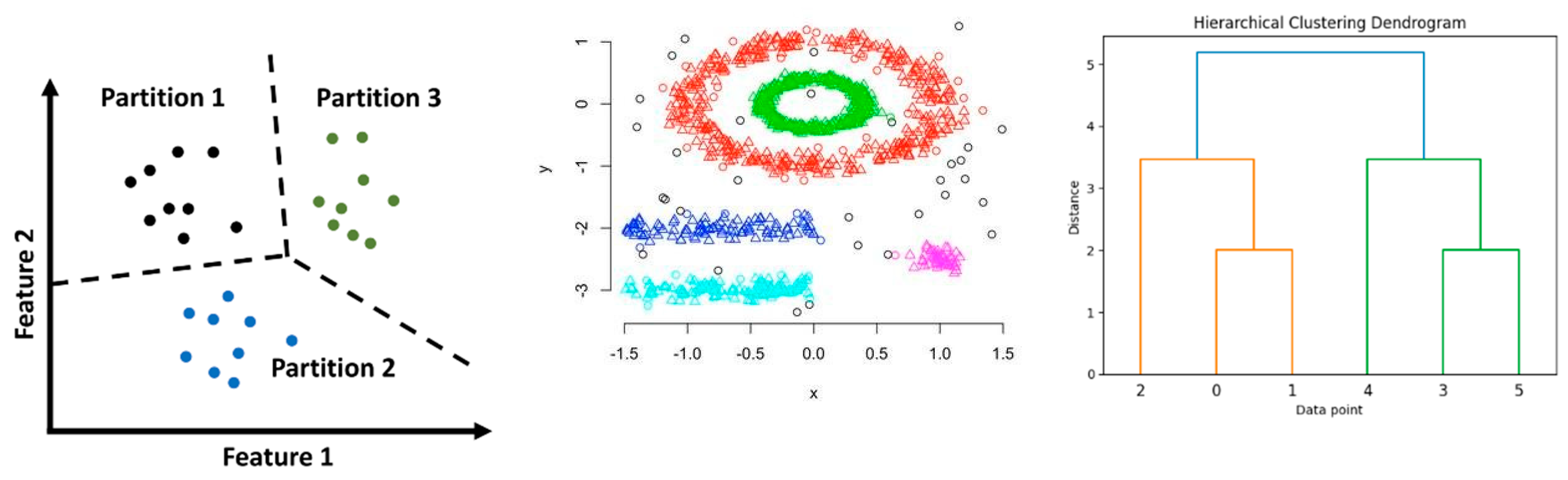
Clustering has been defined as an unsupervised learning method that detects patterns and groups similar data objects in unlabeled data. Within this thesis, its various methods are explored as clustering methods that are appropriate at objective level to different data properties.

Partitioned clustering such as K-Means algorithm has the capability of partitioning data to produce non-overlapping subsets. K-Means is the most efficient as it tries to group data points while minimizing the variance across clusters. K-Means limitations primarily include the prefixed number of clusters and the assumption that data clusters are spherical, which may not be very close to reality.

DBSCAN is an example of density-based clustering, a technique that has advanced to HDBSCAN (Hierarchical Density-Based Spatial Clustering of Applications with Noise), which can discover clusters in arbitrary shapes by finding regions with high densities of points. HDBSCAN builds such a hierarchical structure over an execution of the DBSCAN algorithm in order to select the most stable clusters based on variation in density levels; thus, offering a much better robustness concerning complex data.

Figure 1. Clustering Method.

Figure 1. Clustering Method.

Used Algorithms for the Study

The aim of this study is to analyze the profiles of victims of accidental drug-related deaths by classifying them based on demographic information and patterns of drug use. The data set has both categorical (e.g., race, drug type) and numeric (e.g., age) features, and hence it is suitable for clustering analysis despite its complex nature.

K-Means Clustering is employed due to its speed and efficiency in clustering large data. It effectively clusters individuals quickly based on demographic and drug use characteristics, which helps in the Elbow Method and Silhouette Score being employed to determine the optimal number of clusters, allowing for the identification of substantial high-risk populations. K-Means assumes, however, that the clusters are spherically shaped and of equal size, which may not always be true for real-world mortality data.

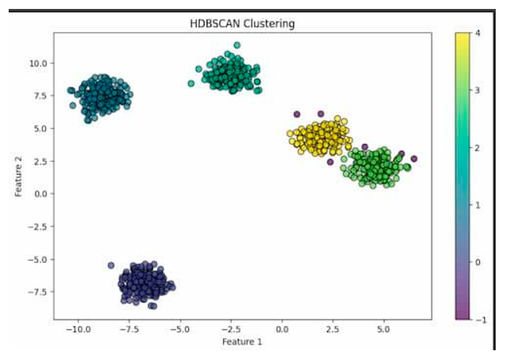
HDBSCAN, however, offers a more flexible solution in that it discovers clusters of various densities and performs well with noise. It is particularly well-suited to study drug-related deaths, which normally display uneven and complex patterns of distribution. HDBSCAN does not require the user to specify the number of clusters in advance, unlike K-Means. This makes it more natural to apply in unstructured and heterogeneous real-world data. Its ability to identify invisible and meaningful structures makes it appropriate in public health uses, in which the victim profiles' clumping may be far from linear or geometric patterns (McInnes et al., 2017).

In this study, a hybrid cluster approach is adopted by combining K-Means and HDBSCAN. By doing so, the computational complexity of K-Means and the robustness and resilience of HDBSCAN are leveraged to assist in the identification of sweeping and subtle trends in the data on accidental drug-related deaths.

Figure 2. KMeans Clustering.

Figure 2. KMeans Clustering.

Figure 3. HDBSCAN.

Figure 3. HDBSCAN.

Pre-Processing Clustering

A thorough pre-processing phase initiated the entire clustering pipeline, which was focused on rendering the dataset clean, consistent, and appropriate for giving out reasonable clusters. Denoising, irrelevant information removal, redundancy, and transformation were initiated to enable similarity-based clustering for datasets. First, the data frame was filtered upon allowed values. Multiple types of dates were included in the dataset: date of death, reported date, and injury date. It was considered analytical consistency; hence, instances were filtered down to only those with a "date of death." With regard to sex, entries accepted as valid were "male" and "female." For categorizing race, “White,” “Black,” and “Black or African American” were retained, which had predominated the records and thus provided a sufficient data base for modeling. Specific cities for residence and death were selected for obtaining further insights into geographic patterns. The filtering procedures, thus, helped remove missing, ambiguous, and low-frequency values that would have introduced noise into and distorted the cluster.

Second, columns which were unnecessary were dropped. These included geographic information like DeathCityGeo and ResidenceCityGeo, which were not in line with the purpose of the study. Unnecessary variables like "Any Opioid" and "Other Opioid" were dropped to avoid overrepresentation of certain substances. Furthermore, non-numeric or less essential columns such as "Cause of Death" and "Description of Injury" were also dropped to maintain the focus on demographic and substance-use attributes suitable for clustering.

To reduce redundancy and improve consistency, the race column was shortened. Text forms like "Black" and "Black or African American" were merged into one category, and "White" was left as a separate group. Bringing this column into alignment with a uniform string format removed inconsistency and prevented spurious fragmentation of results in clustering caused by superficial label differences.

The second was to extract drug-related columns and carry out binary imputation. All columns related to drug use were standardized into binary: 1 indicating the presence of the substance, and 0 indicating its absence. Standardization improved readability and accuracy of similarity computation. It also avoided issues caused by varying input texts. Following that, the dataframe's index was reset so that the structural consistency was maintained and indexing mistakes were avoided during processing.

Following this, feature encoding was used to convert the categorical features into a numerical equivalent which was clustering algorithm-compatible. One-hot encoding was used to create binary flags for each unique category without creating artificial ordinal relationships. The binary columns were converted to integer types for improved memory and computational efficiency. Following the conversion, the encoded features were merged with the existing numerical attributes to produce an entirely processed and merged dataset. Once again, resetting the index guaranteed structural stability. This cautious conversion allowed all the features to contribute equally to the calculation of similarity, which made the results more accurate and interpretable.

Lastly, scaling and normalization were done in order to further refine the data. MinMaxScaler was applied in scaling the age variable so that it would be on par with the binary features and not dominate the similarity calculations. As most of the variables were binary, hamming distance was utilized to measure pairwise similarity. When the occurrence of mixed data types (binary and numeric) required to be used, Gower distance was implemented, as it is specifically optimized for that requirement. The final similarity measure utilized a weighted composite: Hamming and Gower distances both with 45% weighting, to which age only received a diminished 10% weighting in an effort to neutralize its impact. Diagonal entries in the final distance matrix were set to zero and normalized such that each instance had zero distance from itself. This advanced similarity computation method enhanced clustering precision by balancing different types of features and optimizing clustering algorithm performance.

Outlier Detection Model Implementation

Anomaly Detection Methods

Anomaly detection is one of the primary unsupervised learning methods used in this study to detect rare or unusual patterns in the data regarding drug-related deaths. Data mining techniques are critical in finding useful information from huge datasets, and anomaly detection plays a central role in identifying exceptional cases. Three primary anomaly detection algorithms were employed in this project: One-Class SVM, Isolation Forest, and Local Outlier Factor (LOF). These methods were applied particularly for the detection of geographic anomalies, where the place of occurrence was not as it should be and could reflect corridors of drug trade, emergency delays, or irregular use locations.

One-Class SVM

The One-Class SVM (Schölkopf et al., 2001) is a socially supervised algorithm used for anomaly detection that learns a decision boundary about "normal" data and flags points outside the boundary as anomalies. It can efficiently handle high dimensional data with kernel functions such as the radial basis function (RBF) and is particularly favorable of non-linear shapes in the spatial distributions (Tax & Duin, 2004). Drug-related deaths demonstrate geographical outliers that can reflect strange sites of overdose, injury, or residence and even hint systemic or behavioral deviations (Amer et al., 2013).

To implement One-Class SVM, firstly clean the dataset by removing duplicates and extracting only geographic features such as ResidenceCityLAT, ResidenceCityLON, InjuryCityLAT, InjuryCityLON, DeathCityLAT, and DeathCityLON into the drug_outlier_geo dataframe, before applying nu=0.02 to train the model against the expected relative amount of outliers, the rbf kernel for its ability to model non-linear relationships and gamma=0.001 to set how much influence each data point has. The model classifies each instance as either normal (1) or anomalous (-1). The anomaly index was then used to retrieve extreme geographic outlierswhere the death location is greatly different from the residence or injury sites.

Isolation Forest

Isolation Forest is an ensemble-based algorithm that recursively partition data using random splits to isolate anomalies (Liu et al., 2008). Because of their sparsity, anomalies are isolated faster than normal points, which makes the approach very effective for large and high-dimensional datasets without making any distance or density assumptions (Liu et al., 2012). This method is suitable in this study for identifying spatial outliers stemming from unusual travel patterns, exaggerated overdoses, or undocumented drug-use zones.

The model was trained using the same set of geographic features as used in the One-Class SVM implementation. Parameters were set with n_estimators=50 for the number of trees and contamination=0.02 for the expected proportion of anomalies. Random_state=42 was used for reproducibility. The model classified the observations as either normal (1) or anomalous (-1), thus aiding in the isolation of outlier patterns from within the spatial configuration of the drug-related death data, similar to the One-Class SVM.

Local Outlier Factor (LOF)

Local Outlier Factor (LOF) is a density-based approach that identifies anomalies by comparing the local density of each data point with that of its neighbors (Breunig et al., 2000). Unlike global anomaly detectors, LOF can identify subtle, context-dependent outliers and is therefore highly suitable to datasets with locally varying densities (Kriegel et al., 2009). This makes it a useful instrument in detecting weak geographic anomalies in drug-related mortality data, such as unexpected clusters in otherwise low-incidence areas. These may represent emerging drug-use hotspots or local trafficking routes (Campos et al., 2015).

These same geographical attributes (drug_outlier_geo) were preprocessed and trained. The LOF model was initialized with n_neighbors=20 to define the size of the neighborhood, contamination=0.03 to define the proportion of anomalies expected, and novelty=False for unsupervised anomaly detection. The model marked outliers as (-1) and inliers as (1), enabling the identification of local geographic outliers that would not be apparent with global models.

All three of these complementary approaches together present a strong paradigm for detecting spatial outliers in drug mortality data. By utilizing One-Class SVM's non-linear boundary detection capability, Isolation Forest's recursive partitioning ability, and LOF's local density variability sensitivity, the research offers complete and correct detection of geographic anomalies and their potential public health and policy relevance.

Evaluation and Validation of Models

The evaluation models—classification, clustering, and anomaly detection—were assessed through quantitative metrics as well as qualitative interpretation for the holistic understanding of their use in the drug-related overdose.

Classification Model Discussion

In the models tested for classification support vector machine (SVM) with an RBF kernel was the best-balanced and most reliable. With a 92.87% overall accuracy, it displayed almost a strong ability to generalize itself without overfitting as seen in Random Forest (98.22%) and KNN (99.97%) models exhibiting overfitting with minority class performance. Its greatest advantage lies in its ability to handle imbalanced datasets and nonlinear relationships during hyperparameter tuning (C and gamma) and class weights adjustment.

Although Random Forest worked perfectly and gave useful feature importance ideas about dominating class predictions, the model had been leaking due to the very high correlation between the input features and target variable (for example, age group encoded). KNN also had quite impressive performance metrics but could not generalize; it worked like memorization and performed poorly on minority classes and high-dimensional datasets. Execution time comparisons also showed that KNN was the fastest, while the computation time of SVM justified enough its reliability in prediction over various class distributions.

Clustering Model Discussion

For unsupervised learning, HDBSCAN and KMeans were employed to determine behavioral and demographic patterns in drug mortality. While KMeans was satisfactory with a Silhouette Score of 0.3276 and Calinski-Harabasz Index of 1913.19, it was constrained by being able to accommodate only spherical clusters and requiring predefinition of the number of clusters. HDBSCAN, on the other hand, yielded more meaningful clustering results with a better Silhouette Score of 0.5802 and greater intra-cluster similarity and inter-cluster separation. Its noise robustness and ability to handle non-convex cluster shapes made it particularly well-suited to real data with complex spatial and demographic arrangements.

Visualizations using UMAP and cluster-specific heatmaps also established that HDBSCAN identified more significant clusters, particularly in data with irregular patterns of drug use. Although KMeans had more distinct separations in PCA-reduced space, it could not deal with noise, which is inherent in overdose data. The strength of HDBSCAN was its capacity to filter out noise points and concentrate on cohesive, high-density patterns.

Anomaly Detection Model Discussion

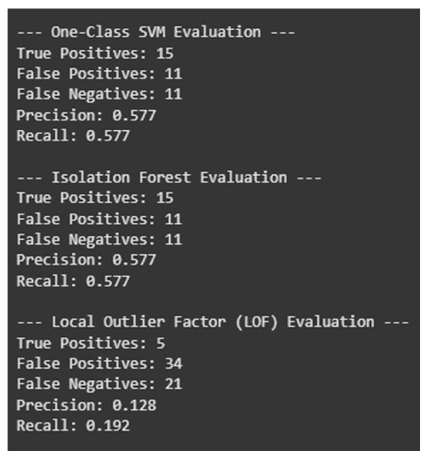
Anomaly detection models were tested on their ability to identify outliers in geographic distance—i.e., the distance between home and location of death. Three methods were compared: One-Class SVM, Isolation Forest, and Local Outlier Factor (LOF). They were compared against a statistical baseline using IQR and 3-Sigma methods.

One-Class SVM and Isolation Forest performed similarly, each identifying 26 geographic anomalies and achieving a balance between true positives and false positives (15 TP, 11 FP). LOF was most sensitive, as it detected the most anomalies (39), but this sensitivity was at the expense of more false positives (34 FP, 5 TP only), reducing its precision. Although LOF's sensitivity is useful for exploratory analysis, the lack of precision makes it less effective for real-time anomaly detection where false alarms are costly.

Geographic outlier plots indicated how these anomalies relate to potential drug trafficking pathways or medical response deserts. Flags on long-distance overdose fatalities—often from out-of-state—indicated systemic issues such as drug tourism or structural barriers to timely medical care. SVM and Isolation Forest yielded more precise, stable anomaly flags and are therefore preferable in contexts where accuracy is paramount.

VISUALIZATION FOR COMPARISON OF ANOMALIES BY EACH MODEL:

When comparing the performance of anomaly detection, the results demonstrate that One Class SVM and Isolation Forest achieve a reasonable balance between detection power (false negative rate) and precision (false alarm rate) with 15 true positives (TP) and 11 false positives (FP) for this dataset. However, the Local Outlier Factor (LOF) has a very high sensitivity and a tendency to significantly over-detect anomalies, along with a very low precision (5 TP and a respectable 34 FP). These results demonstrate the advantages of One-Class SVM and Isolation Forest in terms of accuracy and balance of reliability. They also demonstrate that, despite the fact that LOF detection covers a more general spectrum with less precision, the bridge constructed in each feature space connects these combinations [28,29].

EXECUTION TIME COMPARISON

These two charts demonstrate the comparison of the execution times of different data mining algorithms. The radar chart shows the representation of the three classification algorithms-KNN, SVM, Random Forest.

Figure 4. Execution Time Comparison.

Figure 4. Execution Time Comparison.

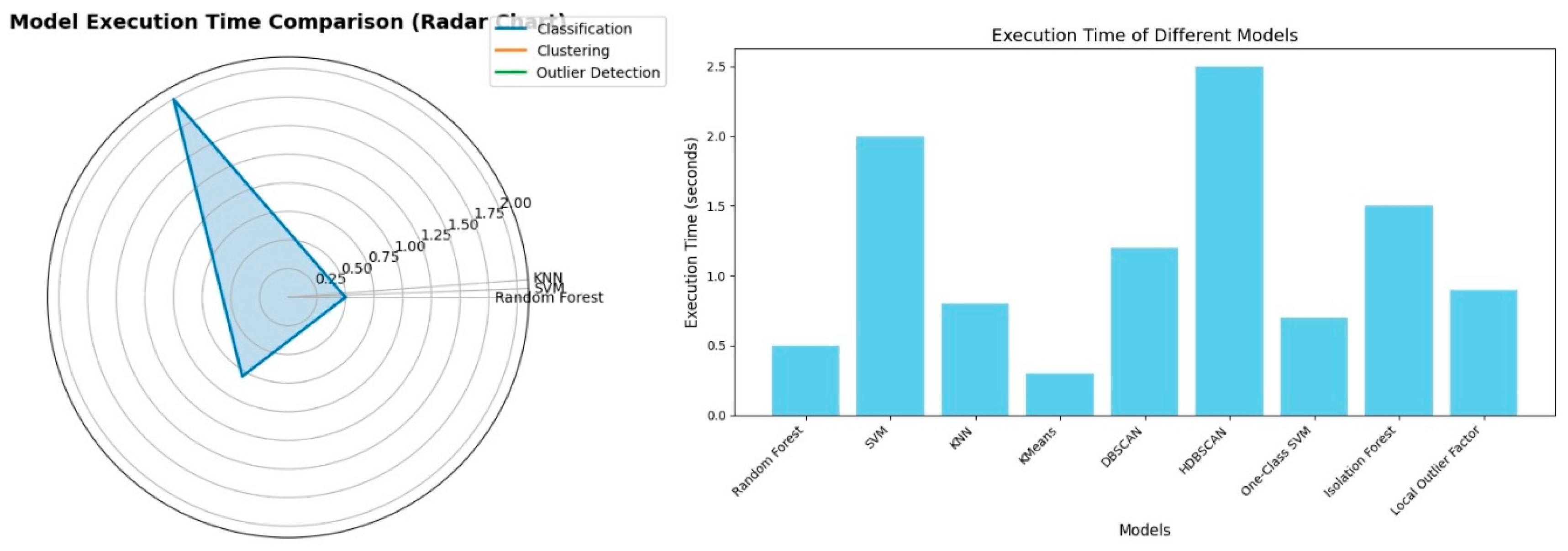
The bar chart illustrates a straightforward comparison of the execution times of all the algorithms. We can directly interpret from the chart:

• HDBSCAN has the highest execution time
• KMeans has the lowest execution time

This direct comparison helps in determining the computational costs of all these algorithms, being crucial parameter for efficient modelling.

5. Conclusions

This study employed an integrative data mining approach—embracing classification, clustering, and anomaly detection algorithms—to detect patterns in accidental drug-related fatalities. Through the utilization of a comparative machine learning model analysis, the research recognized significant demographic risk factors, spatial displacement trends, and distinct substance use clusters.

Among classification models, SVM Kernel was optimum at predicting high-risk age groups due to the fact that it possesses generalization capacity and evenly balanced performance across classes. It was successful at classifying high-risk age groups such as adolescents (10–19) and old (80–89), supporting its effectiveness in strategizing age-specific public health interventions.

Clustering analysis revealed HDBSCAN as more suitable for real-world overdose datasets that are noisy and have complex, irregular distribution patterns. It outperformed KMeans at capturing density-based clusters and did not cluster uncertain points, thereby enhancing interpretability and policy relevance.

For anomaly detection, both One-Class SVM and Isolation Forest performed strongly, identifying geographic outliers that may foreshadow underlying socioeconomic vulnerabilities, trafficking flows, or emergency response failures. LOF, while sensitive, was also subject to over-detection and thus better suited to exploratory application rather than operational implementation.

In conclusion, the combination of supervised and unsupervised machine learning algorithms has been instrumental in unraveling the complexity of drug-related mortality. The findings have immense implications in public health policy, law enforcement, and harm reduction strategies. Future studies may involve the incorporation of models in real time, consulting with domain experts for validation, and extension of analysis to include social determinants and longitudinal follow-up for policy effect assessment.

Figure 5. Venn Diagram of Outliers Detected by Different Methods.

Figure 5. Venn Diagram of Outliers Detected by Different Methods.

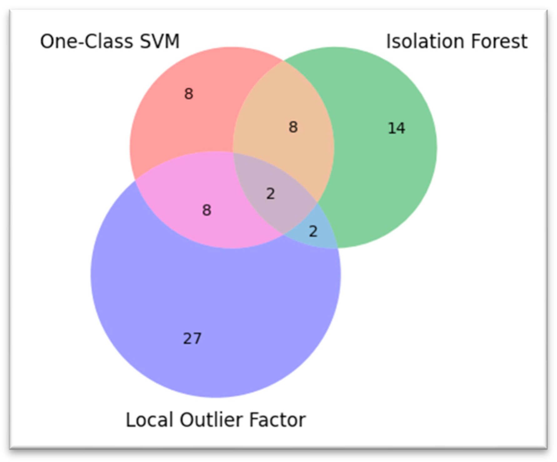
Figure 6. Performance Evaluation.

Figure 6. Performance Evaluation.

References

- Barnett, V. , & Lewis, T. (1994). Outliers in statistical data (3rd ed.). John Wiley & Sons.
- Aggarwal, C.C. Outlier Analysis; Springer Nature: Dordrecht, GX, Netherlands, 2017. [Google Scholar]
- Hawkins, D.M. Identification of Outliers; Springer Nature: Dordrecht, GX, Netherlands, 1980. [Google Scholar]
- Anselin, L. The Local Indicators of Spatial Association—LISA. Geogr. Anal. 1995, 27, 93–115. [Google Scholar] [CrossRef]
- Leys, C.; Ley, C.; Klein, O.; Bernard, P.; Licata, L. Detecting outliers: Do not use standard deviation around the mean, use absolute deviation around the median. J. Exp. Soc. Psychol. 2013, 49, 764–766. [Google Scholar] [CrossRef]
- Breunig, M.M.; Kriegel, H.-P.; Ng, R.T.; Sander, J. LOF: Identifying density-based local outliers. In Proceedings of the 2000 ACM SIGMOD International Conference on Management of Data, Dallas, TX, USA, 15–18 May 2000; pp. 93–104. [Google Scholar] [CrossRef]
- Liu, F.T.; Ting, K.M.; Zhou, Z.-H. Isolation forest. In Proceedings of the 2008 Eighth IEEE International Conference on Data Mining, Pisa, Italy, 15–19 December 2008; pp. 413–422. [Google Scholar] [CrossRef]
- Xu, D.; Tian, Y. A Comprehensive Survey of Clustering Algorithms. Ann. Data Sci. 2015, 2, 165–193. [Google Scholar] [CrossRef]
- McInnes, L.; Healy, J.; Astels, S. hdbscan: Hierarchical density based clustering. J. Open Source Softw. 2017, 2. [Google Scholar] [CrossRef]
- Al-Mejibli, I.S.; Alwan, J.K.; Abd, D.H. The effect of gamma value on support vector machine performance with different kernels. Int. J. Electr. Comput. Eng. (IJECE) 2020, 10, 5497–5506. [Google Scholar] [CrossRef]
- Semantic Scholar. (2015). Optimal γ and C for ε-Support Vector Regression with RBF Kernels. https://www.semanticscholar.org/reader/a80895eaf5a210027a10eccf265e6a8c2d22102d.
- Dogra, V. , Singh, A., Verma, S., Kavita, Jhanjhi, N. Z., & Talib, M. N. (2021). Analyzing DistilBERT for sentiment classification of banking financial news. In S. L. Peng, S. Y. Hsieh, S. Gopalakrishnan, & B. Duraisamy (Eds.), Intelligent computing and innovation on data science (Vol. 248, pp. 665–675). Springer. [CrossRef]
- Gopi, R.; Sathiyamoorthi, V.; Selvakumar, S.; Manikandan, R.; Chatterjee, P.; Jhanjhi, N.Z.; Luhach, A.K. Enhanced method of ANN based model for detection of DDoS attacks on multimedia internet of things. Multimedia Tools Appl. 2021, 81, 26739–26757. [Google Scholar] [CrossRef]
- Chesti, I. A. , Humayun, M., Sama, N. U., & Jhanjhi, N. Z. (2020, October). Evolution, mitigation, and prevention of ransomware. In 2020 2nd International Conference on Computer and Information Sciences (ICCIS) (pp. 1–6). IEEE.
- Alkinani, M.H.; Almazroi, A.A.; Jhanjhi, N.; Khan, N.A. 5G and IoT Based Reporting and Accident Detection (RAD) System to Deliver First Aid Box Using Unmanned Aerial Vehicle. Sensors 2021, 21, 6905. [Google Scholar] [CrossRef] [PubMed]
- Babbar, H.; Rani, S.; Masud, M.; Verma, S.; Anand, D.; Jhanjhi, N. Load Balancing Algorithm for Migrating Switches in Software-defined Vehicular Networks. Comput. Mater. Contin. 2021, 67, 1301–1316. [Google Scholar] [CrossRef]
- Aldughayfiq, B.; Ashfaq, F.; Jhanjhi, N.Z.; Humayun, M. YOLOv5-FPN: A Robust Framework for Multi-Sized Cell Counting in Fluorescence Images. Diagnostics 2023, 13, 2280. [Google Scholar] [CrossRef] [PubMed]
- Ashfaq, F.; Ghoniem, R.M.; Jhanjhi, N.Z.; Khan, N.A.; Algarni, A.D. Using Dual Attention BiLSTM to Predict Vehicle Lane Changing Maneuvers on Highway Dataset. Systems 2023, 11, 196. [Google Scholar] [CrossRef]
- Javed, D.; Jhanjhi, N.; Khan, N.A.; Ray, S.K.; Al Mazroa, A.; Ashfaq, F.; Das, S.R. Towards the future of bot detection: A comprehensive taxonomical review and challenges on Twitter/X. Comput. Networks 2024, 254. [Google Scholar] [CrossRef]
- Das, S. R. , Jhanjhi, N. Z., Asirvatham, D., Ashfaq, F., & Abdulhussain, Z. N. (2023, February). Proposing a model to enhance the IoMT-based EHR storage system security. In International Conference on Mathematical Modeling and Computational Science (pp. 503-512). Singapore: Springer Nature Singapore.
- Alshudukhi, K.S.S.; Ashfaq, F.; Jhanjhi, N.Z.; Humayun, M. Blockchain-Enabled Federated Learning for Longitudinal Emergency Care. IEEE Access 2024, 12, 137284–137294. [Google Scholar] [CrossRef]
- Jhanjhi, N. Z. , & Shah, I. A. (Eds.). (2024). Navigating Cyber Threats and Cybersecurity in the Logistics Industry. IGI Global.
- Srinivasan, K.; Garg, L.; Chen, B.-Y.; Alaboudi, A.A.; Jhanjhi, N.Z.; Chang, C.-T.; Prabadevi, B.; Deepa, N. Expert System for Stable Power Generation Prediction in Microbial Fuel Cell. Intell. Autom. Soft Comput. 2021, 29, 17–30. [Google Scholar] [CrossRef]
- Saeed, S. , Abdullah, A., Jhanjhi, N. Z., Naqvi, M., & Ahmad, M. (2022). Optimized hybrid prediction method for lung metastases. In Approaches and Applications of Deep Learning in Virtual Medical Care (pp. 202-221). IGI Global Scientific Publishing.
- Saeed, S.; Jhanjhi, N.; Abdullah, A.; Naqvi, M. Current Trends and Issues Legacy Application of the Serverless Architecture. Int. J. Comput. Netw. Technol. 2013, 6, 100–108. [Google Scholar] [CrossRef]
- Shah, I.A.; Jhanjhi, N.; Brohi, S. (2024). Cybersecurity issues and challenges in civil aviation security. Cybersecurity in the Transportation Industry, 1-23.
- Zaman, D. N. , & Memon, N. A. ( 3(2), 120–127.
- Zaman, N. , Rafique, K., & Ponnusamy, V. (Eds.). (2021). ICT Solutions for Improving Smart Communities in Asia. IGI Global.
- Shah, I. A. , Jhanjhi, N. Z., & Ray, S. K. (2024). IoT Devices in Drones: Security Issues and Future Challenges. In Cybersecurity Issues and Challenges in the Drone Industry (pp. 217-235). IGI Global.
Disclaimer/Publisher’s Note: The statements, opinions and data contained in all publications are solely those of the individual author(s) and contributor(s) and not of MDPI and/or the editor(s). MDPI and/or the editor(s) disclaim responsibility for any injury to people or property resulting from any ideas, methods, instructions or products referred to in the content. |
© 2025 by the authors. Licensee MDPI, Basel, Switzerland. This article is an open access article distributed under the terms and conditions of the Creative Commons Attribution (CC BY) license (https://creativecommons.org/licenses/by/4.0/).
Copyright: This open access article is published under a Creative Commons CC BY 4.0 license, which permit the free download, distribution, and reuse, provided that the author and preprint are cited in any reuse.