Submitted:
01 September 2025
Posted:
02 September 2025
You are already at the latest version
Abstract
This research project addresses the use of data mining techniques for studying accidental opioid-related deaths in the United States using the "Accidental_Drug_Related_Deaths" dataset. More specifically, we seek to identify the distinctions in patterns and associated factors between accidental overdose incidents and intentional overdose incidents (suicide, undetermined intent, homicide). During the time period being analyzed, we determined that there were more than 90% of overdose deaths that were classified as accidental in 2022. The main goal of this project is to utilize classification models to predict whether or not opioids are likely to be involved in an incident of overdose based on the identifying features of the demographic and situational features. This prediction will allow for more timely and targeted medical interventions with the individuals experiencing an overdose incident. The analysis considers class imbalance, using SMOTE-Tomek Links, models each of the classification in a single analysis, including, Random Forest, XGBoost, Logistic Regression, SVM, and MLP Classifier, while hyper-parameter tuning the models toward maximum recall. In addition to the classification models, we applied several algorithms for anomaly detection (OneClassSVM, Isolation Forest, Elliptic Envelope) to describe the possibility of rare drug combinations that could be potentially dangerous. Overall, we demonstrated that when handled carefully, there is a range of preprocessing, feature selection, and machine learning approaches for anomaly detection that made it possible to better identify risk factors for opioid-related overdose, which could be used to support a public health-based area of intervention, data-driven programming for states that are facing the opioid crisis.
Keywords:
SMOTE-Tomek
; Links
; Class
; SVM
1. Introduction
Drug overdose deaths in the United States represent a significant and sustained public health emergency closely associated with the issue of drug addiction that is pervasive in our country. The majority of these drug overdose deaths are unintentional deaths rather than deaths from intentional self-harm. Data from 2022 show that 92.3% of reported drug-related deaths were due to "accidental" overdose deaths, in comparison to deaths by "suicide," "undetermined," or "homicide," which occur at much fewer rates. The high percentage of accidental deaths indicates the complexity and seriousness of the problem both medically and socially. In order to combat an issue of that size, addressing the issue requires more than recognizing its scale; it requires recognition of the patterns that contribute to unintentional drug-related deaths and ultimately the risk factors that occur. While unintentional deaths may seem random, once analyzed, they may show various trends, or different factors could suggest some commonality amongst them which would inform preventative measures [1,2]. The hard part is identifying these patterns systematically in large complex datasets and this is where data mining can prove useful.
In this research, we used methods from data mining to analyze the Accidental Drug Related Deaths dataset to generate valuable insights in relation to incidental overdose cases in the United States. Post a rigorous data pre-processing stage that related to class imbalance and feature creation. This study assessed the extent to which the use of predictive modelling could estimate the probability of opioid involvement in overdose cases where we had access to demographic and situational features. This is particularly salient as the current issues related to drug overdoses are becoming increasingly alarming, particularly with ever-higher doses of synthetic opioids such as fentanyl becoming available on the black market. In 2022 alone there were approximately 108,000 reported drug deaths in the U.S., with opioid involvement featured in around 76% of those cases. More accurate and time-critical identification of the substances involved in an overdose is important to the quality of any treatment by a clinician, and naloxone would be a specific intervention whereby identifying the agent(s) in a timely manner could save a life with very limited resources and time [3,4,5,6,7,8]. The addition of predictive analytics improves clinical decision-making time, and subsequently, supports the effective use of scarce resources in an emergency medical environment, potentially saving lives. Understanding the demographic, geographic, and healthcare access demographics can also improve decision-making for authorities in where it can manage resources and provide more tailored responses to act to reduce risk in the at-risk area/communities. The report will discuss the specifications and investigation of several machine learning models such as Random Forest, XGBoost, Logistic Regression, Support Vector Machine, Artificial Neural Networks, to classify opioid involvement, and any robust methodologies employed to overcome class imbalance and data leakage in the fit methods [9,10,11,12]. It will also provide an examination of the application of the previous anomaly detection algorithms' capabilities of identifying uncommon and potentially unsafe drug combinations to inform preventative actions. By meticulously implementing high-quality data mining and machine learning methods, this project could provide a better understanding of accidental drug-related deaths in the United States and could also be able to produce applied knowledge that has the potential to inform clinical practice and public health policy.
The issue of drug overdose deaths in the U.S., as it correlates with drug addiction issues, is a large problem. Drug overdose deaths can either be intentional (i.e., suicides) or unintentional. Research indicates, however, that most drug overdose deaths are unintentional (i.e. the individual was not aiming to kill themselves, however, they did it by accident). For instance, a thorough study on the subject area in 2022 showed that of the drug-related deaths in the year, 92.3% of them were classified as unintentional, while only 4.5% were classified as a suicide, and 3.0% undetermined, with under 1.0% as a homicide [13,14,15,16].
Nonetheless, the issue of drug-related deaths in the United States is not straightforward, and it has many differences when considering their investigation. Not all observations are coincidental. Yes, some do indeed fall into trends and patterns, and the question is what these patterns are, how they can be understood, and then used to help those responsible make the necessary decisions on action to take on the serious issue of drug overdose deaths in the United States [17,18,19]. This is where the various forms of data mining techniques come into play. In this report, we discussed the implementation of a small number of recognized Data Mining techniques in deriving patterns and conclusions about the problem of accidental drug-related deaths in the United States. We were supplied a dataset referred to as ' Accidental_Drug_Related_Deaths.csv', to conduct our explorations [20,21,22,23,24,25]. This dataset went through general preprocessing before we received it, and we used the cleaned version referred to as 'Accidental_Drug_Related_Deaths_Cleaned.csv 'in applying the recognized data mining techniques. This report details the implementations, results, and visualizations, and evaluates the success of each technique in achieving its intended purpose. This study also refers to the other studies, where this dataset has been used [26,27,28,29,30] directly or indirectly; furthermore, earlier studies [31,32] related to Cloud and LTE as well.
Implementation of Data Mining Techniques
This section is going to address the Python implementation of the aforementioned methods (clustering, anomaly detection and classification), as well as the obstacles involved in the implementation and resolution.
Classification
The classification problem for this problem statement can be summed up as a simple Binary Classification. The objective is to predict whether or not the `any_opioid` column returns 0 (absence) or 1 (presence) for a patient based on their demographics, which are `age`, `sex`, and `race`. The unbalanced nature of the target variable needs to be considered in determining a model focus.
Figure 1.
Target Variable Distribution before SMOTE.
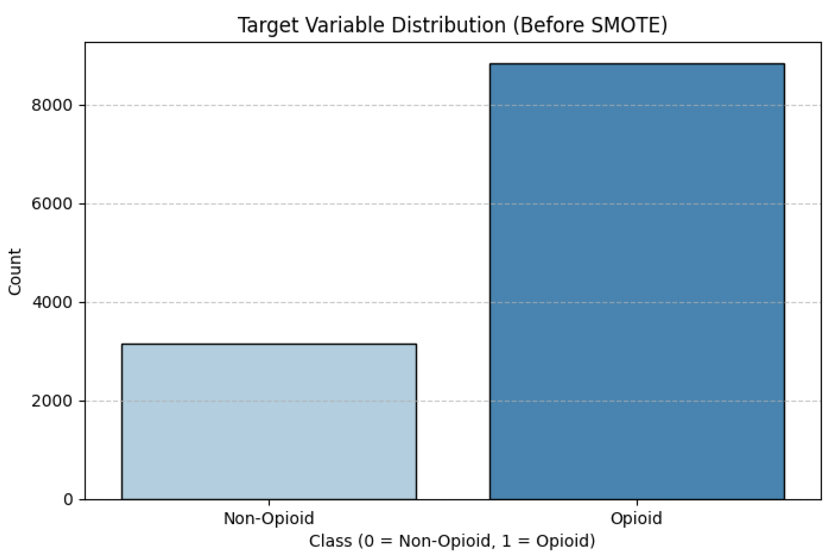
The emphasis is on keeping high recall score or sensitivity, as there are great costs associated with false negatives. A case of opioid involvement that is classified incorrectly as non-opioid related can have fatal consequences. Recall will maximize the number of correct identification of actual opioid cases. In addition, the ramifications of false positives (versus non-opioid deaths being related to opioids) are less consequential because Naloxone does not produce adverse effects in patients who have not used opioids.
Dealing with Dataset Imbalance
Class imbalance in machine learning can lead to biased models that do well on the majority class but are unable to detect the minority class. In this case, opioid related deaths (Class 1) vastly outnumber non opioid deaths (Class 0) as illustrated by the original class disribution, which could lead the model to favor the majority class by simply predicting "Opioid", as this class dominates the dataset.
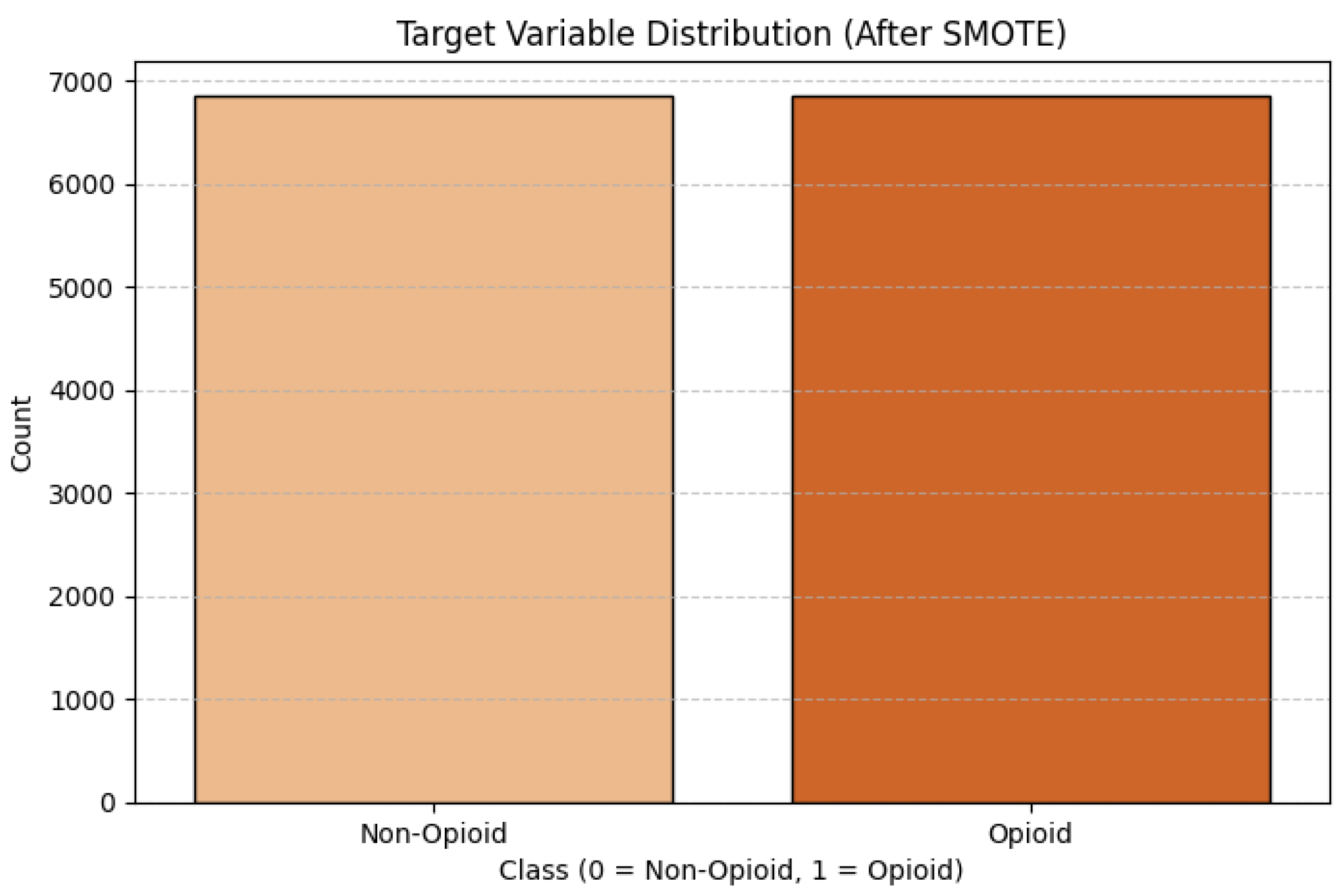
Once again, if this was the case, it is likely that the biased model would achieve optimistic results with a high accuracy by omitting the minority class. For this reason, I shifted my focus on Recall as the metric to measure the capture of opioid related deaths (the better metric to assess the performance.) To avoid these types of problems, the class imbalance must be dealt with appropriately with sampling methods. The sampling method chosen for this project was SMOTE-Tomek Links. SMOTE- Tomek Links is a hybrid sampling method that combines both SMOTE (Synthetic Minority Over-sampling Technique), that balances the data set by creating synthetic samples for the minority class, and Tomek Links (Under-sampling) which cleans up noisy data by removing samples that are close to either side of the decision boundary. This method aimed to create a well-balanced data set while allowing the model to improve generalize. The resulting target variable distribution is:
Figure 2.
Target Variable Distribution after SMOTE.
Addressing Data Leakage
Data leakage is when information from the test set is leaked into the training. Data leakage can lead to overly optimistic performance measures and reduce the model's ability to generalize, which can lead to the model not performing well when being tested with previously unseen data. To prevent this, a few steps were taken in the procedures that targeted data leakage and affect the results.
Binning Latitude & Longitude Values (Feature Engineering)
Instead of providing the actual values for the latitude and longitude the location information can later be put in bins of discrete grades. This is to mitigate the model's ability to use this information as unique identifiers and fully memorize the locations instead of learning from actual meaningful patterns. The binning of the data was conducted prior to the train-test-split to maintain the location-based inferences were generalized and did not leak actual explicit location values into the test set. This will prevent the model from overfitting location-based patterns that do not generalize to new data. The appropriate number of bins was determined using a Freedman-Diaconis rule that uses the equation below to calculate the optimal bin width:
Where IQR is the interquarile range of the dataset and (n) is the any observations in the dataset. We used this strategy to bin the death and injury latitudes but kept the residence latitudes and longitudes intact because there are too many unique values for Residence lat/longs which makes it extremely granular. If residence lat/longs were used within the binning, the model would consider each binned category as a separate feature, resulting in over-binning, which would result in bins that have too much location-specific detail. Over-binning prevents over-fragmentation of data and allows models to learn generalized location patterns rather than memorizing latitudes and longitudes. Excluding residence latitudes and longitudes has some potential disadvantages including lower interpretability of the model. However, we believe these negatives do not outweigh the positives of excluding these features.
Train-Test Split and Scaling Prior to SMOTE-Tomek Application
We split the dataset into two (train, test) prior to SMOTE-Tomek resampling and only applied SMOTE to the training data. SMOTE creates synthetic data points, and we want to avoid having synthetic samples leak, or slip into testing data. This would make testing data dependent on the data dependent learning process, ultimately contributing to the predictive accuracy of the model classifier. We split the data prior to applying SMOTE-Tomek to avoid affecting testing data by changing the training data, and the resulting train, test dataset will allow us to have an unbiased test dataset. The prior to SMOTE dataset, numerical data features were also scaled to allow more compatibility across all models and improved performance due to better stability of training.
GridSearchCV Restricted to the Training Set
Hyperparameter tuning via GridSearchCV was done only on the training set. Therefore, the test data never end up being indirectly seen by the model during training, thus ensuring theTest set remained independent from the model for unbias performance testing.
Independent Model Training for Each Version
We trained distinct model versions to assess the effects of different preprocessing steps and adjustments. Baseline models were trained on raw training data with no resampling, while "SMOTE models" were trained on resampled training data that did not adjust hyperparameters. Each model variant was trained independently (i.e., there were no cross-contaminations without an adjustment) to eliminate any accidental transfer of information or insights between models. This separation will ensure reproducibility and legitimacy for performance comparisons.
Model Selection
Because of the class imbalance in the data, it is important to identify models that work well with imbalanced data and have a balance of robustness, interpretability and prediction power. The following models were selected to provide variety of classification methods so we can compare methods and approaches to address this issue. Five models representing different classes of machine learning algorithms where selected:

Table 1.
Model Selection for Classification.
| Model | Pros | Cons |
| Random Forest | Provides feature importance insights. | Requires more tuning to prevent overfitting. |
| Works well with non-linear relationships present in opioid-related predictors. | Harder to interpret than simpler models. | |
| Less sensitive to outliers than Logistic Regression. | ||
| eXtreme Gradient Boosting (XGBoost) | Optimized for imbalanced datasets. | Prone to overfitting if parameters are not well-tuned. |
| Efficient with large feature spaces which is useful when handling medical data. | Computationally intensive. | |
| Reduces bias-variance tradeoff. | ||
| Logistic Regression | Simple and interpretable, making it easy to explain the results. | Assumes linear relationships, which limits performance due to lack of feature correlation in this dataset. |
| Computationally efficient and easy to deploy. | Struggles with class imbalance. | |
| Support Vector Machine (SVM) | Effective in high-dimensional spaces. | Computationally expensive and long execution time. |
| Finds complex decision boundaries, improving classification accuracy. | Sensitive to noisy data. | |
| MLP Classifier (ANN) | Detects complex, non-linear relationships. | Requires large training data, making it prone to overfitting if not regularized. |
| Learns hierarchical representations, making it useful for demographic correlations. | Computationally demanding, requiring significant resources. |
Feature Selection
Feature importance was done using the attribute `~.feature_importances_` and plotting a bar graph accordingly, for both the base tree-based model and the best performing tree-based models (manual tuning). These models were selected due to their better performance relative to the rest of the models. The following are the results of the graphs:
Figure 3.
Feature Importance Results for Unsampled Data (Random Forest).
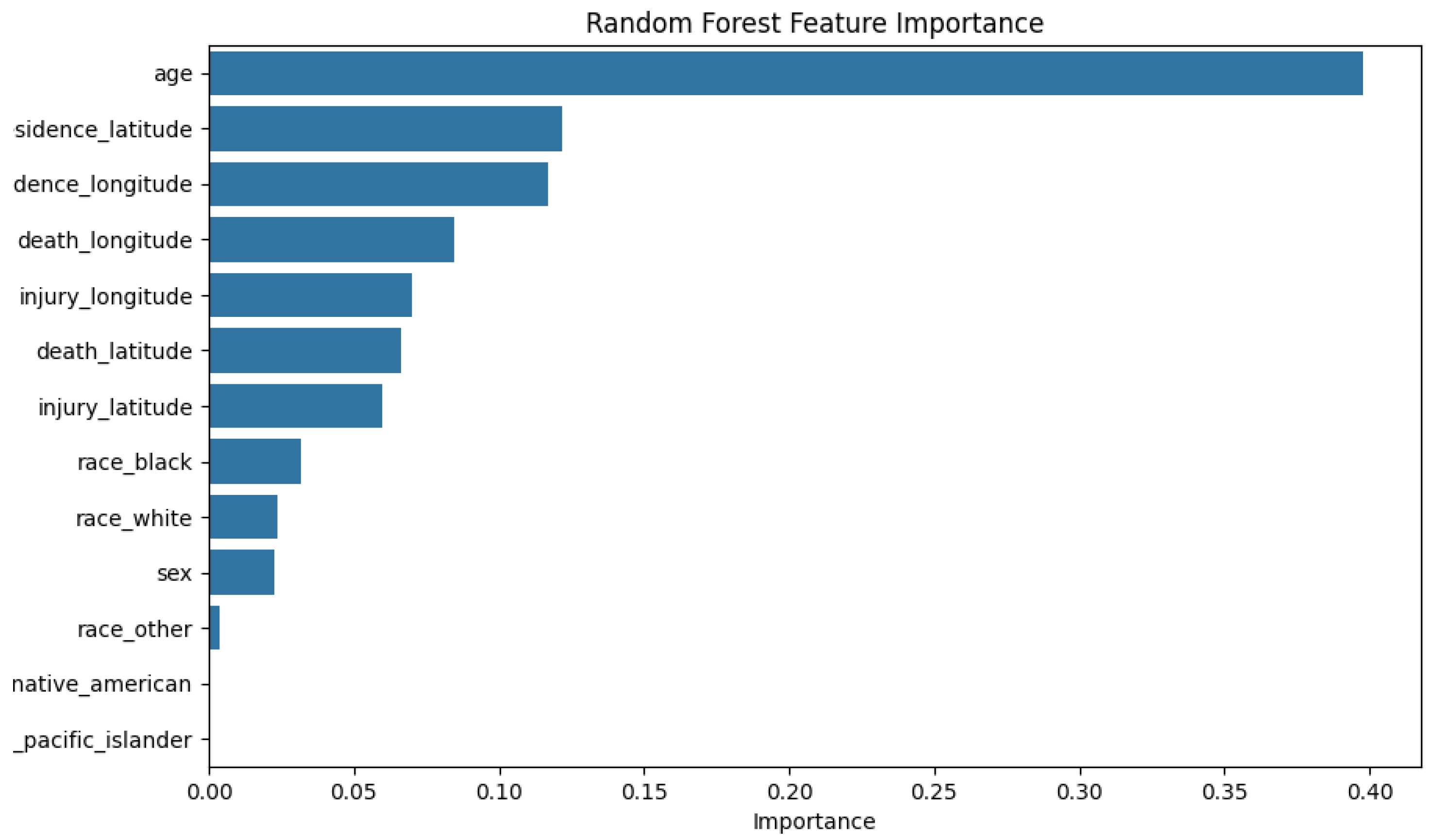
The feature importance of `race_native_american` and `race_pacific_islander` was low (< 0.00) for both models, which was expected since the dataset didn't have enough entries in those categories. With such a small sample, we cannot provide useful patterns which means we will likely ignore these features during training because they will contribute very minimally to classification. Overfitting is a risk because the model could potentially be learning random noise, and not any useful patterns. To lessen that risk these 2 features are planned to be removed. The validation will be used for the Chi-Square Test.
Supervised Model Variants
Physical fitness offers many benefits to the body, and the list of benefits includes lowering the risk for diseases, improving cardiovascular fitness, and managing stress. The office of Health, Nutrition, and Exercise Sciences in 2018, Nystoriak et al. states, regular exercise decreases the cardiovascular mortality rate and risk for cardiovascular diseases. Exercise is a natural way to control or modify many risk factors for heart disease. Things like elevated blood pressure and elevations in cholesterol levels. Additionally, aerobic and strength resistance exercises can provide physiological modification, achieve an improvement for vascular health, and metabolic health to prevent diseases.
Next, you will have trained models with GridSearchCV options, through the GridSearchCV utility used to find optimal hyperparameters to train each model, depending on the recall score used. All combinations of parameters from previously set grids were explored systematically. The best performing options were stored and are as follows: for Random Forest, max_depth=20 and n_estimators=200;for XGBoost, learning_rate=0.1 and max_depth=6; for Logistic Regression, C=10 and penalty='l2'; for SVM, C=10 and a linear kernel; for and ANN, hidden_layer_sizes=(100,), learning_rate_init=0.01 and solver='adam';
After GridSearchCV, a stage of manual tuning was carried out separately, geared towards optimizing to the max through trial and error processes. In the manual tuning processes, changing max_depth to 18, or changing min_samples_split from default of 2 to other values for Random Forest; of xgboost, changes were to gamma and colsample_bytree; of the ANN, located changes on layer size and learning rate; and similarly for logistic regression - changed the penalty term; SVM made no changes as overfitting was a risk with many changes given tuning parameters had all been optimized. Models from the manual tuning process were again evaluated, and their results extracted to a single DataFrame for comparison of new model performance versions across all changes.
Anomaly Detection Process
Data Preparation
Anomaly detection started with relevant drug-related features, including Heroin and Cocaine. Data was transformed to true/false indicator variables, to determine if any drug was present in the case (True) or not present (False). After that, the DrugCount column was created to sum the boolean columns for each row. The DrugCount variable is essentially a count of drugs detected in the case. The investigators reasoned that this binary and count-based framework provided a nice structure to model, and aided in anomaly detection of uncommon or atypical polydrug use cases.
Model Selection
Four distinct algorithms are used in order to capture different kinds of anomalies within the data set: One-Class SVM, Isolation Forest, Elliptic Envelope, and Local Outlier Factor (LOF). Each of these models represents a different approach to anomaly detection. The One-Class SVM model builds a decision boundary around the normal data points in a high-dimensional space and is the best model to manage complex, non-linear patterns, but has known issues tuned against different parameters and high computation. The Isolation Forest model detects anomalies through recursive partitioning strategies and the ability to isolate a single point from the dataset, which makes it scalable and interpretable; however, it uses the contamination parameter to determine which observation should be considered an anomaly, which should be carefully configured for some datasets in order to avoid mislabeled class. Although the algorithm Elliptic confidence assumes that all data in the dataset follow a Gaussian-like distribution, whereby all models based on an elliptical boundary boundary would be in that cluster to represent the central cluster of data, thus it will control when the data is itself follows a Gaussian distribution and elliptical; ultimately, it could be severely affected by outliers if they leak into the training set. The last method is LOF (Local Outlier Factor), this method bases its parameters on factors of local density; the LOF method is largely successful with datasets that have complex and nonuniform structures across class observable. The LOF predict method can include challenges, as it often requires special consideration for accurate deployment.
Real-world datasets tend to be too thin on anomalies to train models well, so we considered synthetic anomaly injection to construct training data. This technique had us randomly selecting 5% of the rows in the dataset, flipping the Boolean feature values to create the artificial anomalies in the dataset, and assigning were labeled -1 for the anomalies and 1 for the normal rows. The exact random seed was utilized to be able to reproduce the processes used to generate synthetic data. The produced feature matrix and label for the synthetic anomaly injection were assigned X_synthetic and y_synthetic to serve as the training and validation datasets for the anomaly detection models and enhance their ability to learn to detect only relatively rare and abnormal patterns.
Supervised Model Variants
The construction of four supervised models allowed us to examine model performance in different scenarios. The Base Models were supervised models, trained on the original dataset without the application of hyperparameter tuning or any resampling methods. The models were trained/tested following the standard 80/20 train/test split, and the performance metrics were recorded separately. The SMOTE Models were supervised models that addressed class imbalance using SMOTE-Tomek resampling, without any hyperparameter tuning; these models would follow the same training and evaluation structure noted above for the base models. The GridSearchCV Tuned Models applied grid search to the training set, where hyperparameter tuning focusing on maximizing the Recall score was performed. The best configuration for each algorithm was saved (e.g., RandomForest, max_depth=20). The Manually Tuned Models utilized slight modification after grid search was completed, in order to optimize performance (i.e., modifying the learning rate for a neural network, or the depth of the tree for ensemble models). Importantly, the SVM model was not subjected to this manual tuning process in order to avoid overfitting.
Anomaly Detection Process
The purpose of the anomaly detection process was to recognize abnormal patterns of polydrug usage in drug use with unsupervised learning techniques. In the Data Preparation Part, Boolean drug-use features from each selected drug column were created, and a DrugCount variable was created to capture the number of drugs detected in each case. In the Model Selection step, four unsupervised models were selected: One-Class SVM because of its flexibility (but highly sensitive to tuning), Isolation Forest because of its scalability and speed, Elliptic Envelope (which assumes Gaussian distribution), and Local Outlier Factor (LOF, which is useful for local anomalies but does not have a standard .predict() method).
The Synthetic Anomaly Injection added artificial anomalies by randomly flipping Boolean values in 5% of the data randomly by a fixed random seed and binary labels to create anomalies to simulate a classification task. Parameter Grids were custom created for each model to guide hyperparameter exploration. A Grid Search with a Custom F1 Scorer (which treats anomalies as the positive class) was implemented for each model using five-fold cross-validation and parallelized usage to identify the best parameter settings.
In the Grid Search Execution phase, every model was tuned on its own, using the associated parameter grid. Several exceptions were made for LOF, regarding its prediction limitations. We saved the best estimators, parameter sets, and the associated F1 scores for our reference later. The Output section indicated that Isolation Forest produced the best F1 score (~0.98), while Elliptic Envelope produced the second-best (~0.85). Both the One-Class SVM and LOF produced significantly lesser F1 scores, notably, LOF seemed to demonstrate symptoms of underfitting.
In the Refitting on Original Data section, we applied the best models of the grid search to the original, unmodified polydrug dataset. Isolation Forest, Elliptic Envelope and One-Class SVM used .fit() then .predict() to develop anomaly labels while LOF, because of the way it is constructed, used .fit_predict(). We stored our predictions within a results dictionary but also added new columns to the original DataFrame for reference against our methods.
Clustering
Clustering was examined as an additional unsupervised approach. The process started with Starting Up. In this phase, the dataset was loaded, and the relevant libraries were imported. The libraries included tools for data manipulation, visualization, clustering (K-Means, DBSCAN, HDBSCAN), preprocessing, and performance evaluation. In the Model Selection phase, K-Means clustering was selected, as it was efficient and scalable; however, it is limited by the requirement to choose k, and it is sensitive to outliers. DBSCAN was selected for its robustness to noise and the lack of need to select k; however, it is sensitive to its parameter settings. HDBSCAN was included to handle varying densities and automatically determine clusters; however, it is computationally intensive. In the Implementation segment, K-Means was performed on standardized geographic coordinates (i.e. death_latitude, and death_longitude) using StandardScaler. The k-clustering assessment involved two approaches for determining the number of clusters: The Elbow Method and the Silhouette Score to determine how well each point fit in its assigned cluster. The two approaches were deemed suitable and were used to determine the best number of clusters for the dataset.
Figure 4.
Elbow Method Graph.
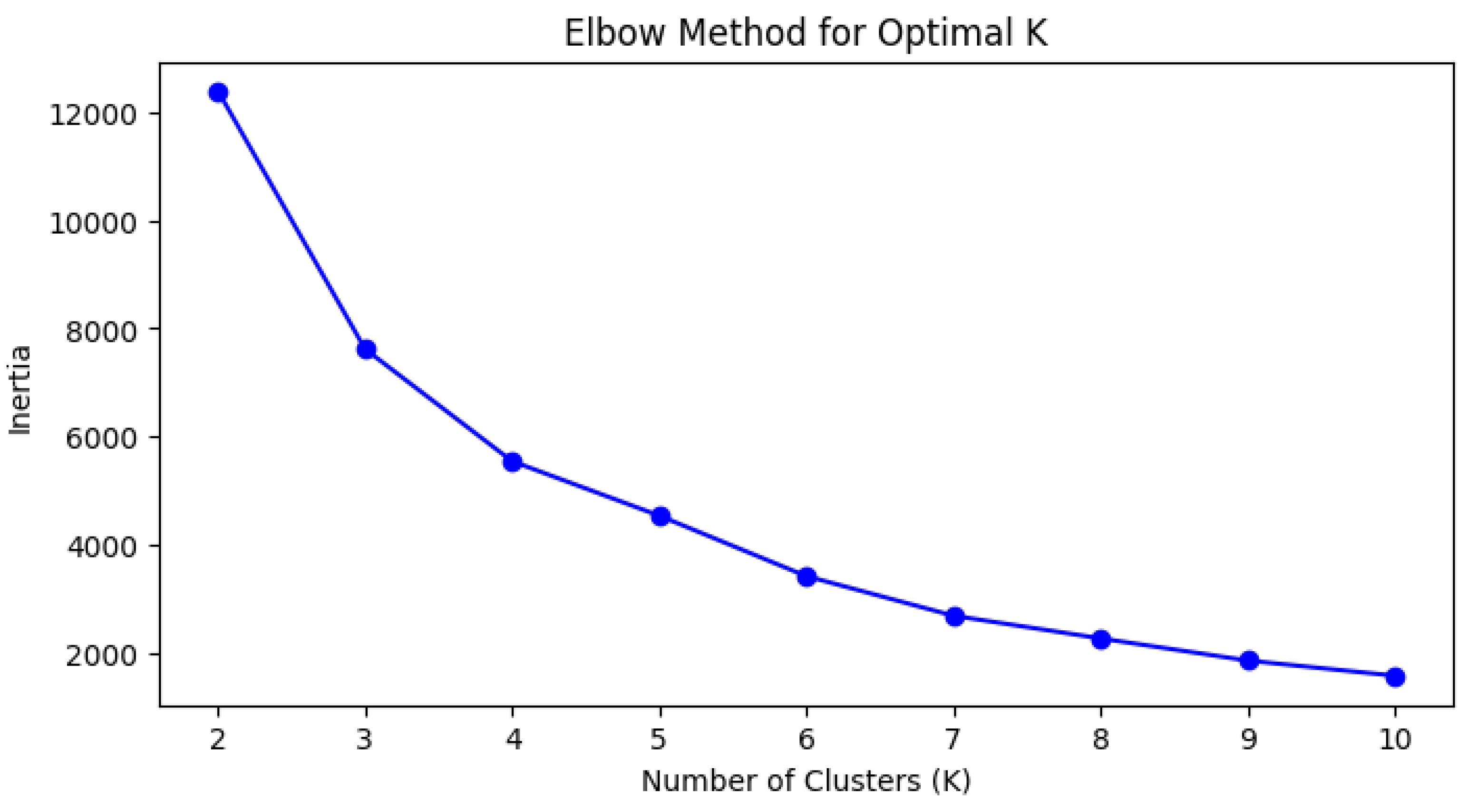
Figure 5.
Silhouette Score Graph.
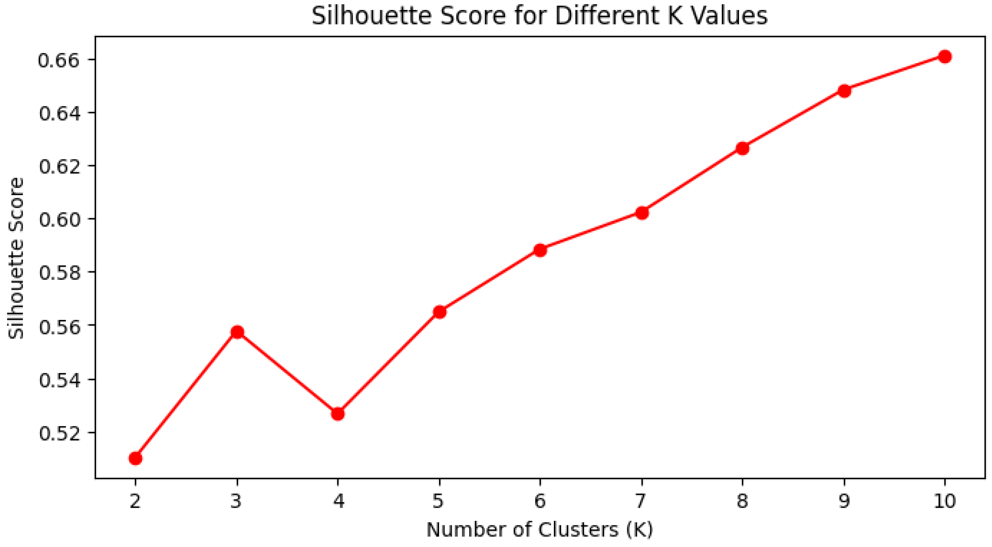
The choice of clustering models and methods was primarily driven by the need to connect the designs to identifiable patterns within the geospatial data with coordinates indicating specific deaths. Given that the number of clusters in K-Means is arbitrary, the Elbow Method and the Silhouette Score were both used to help determine the optimal number of clusters. For example, the inertia was continuously decreasing although the inertia outputs from the Elbow Method and the Silhouette Score fluctuated across different numbers of clusters. The inertia was decreasing as the number of clusters was increasing while the Silhouette Score increased from k = 2 to k = 3, decreased at k = 4, and then increased again from k = 5 and higher. The evaluation of clusters considered both compactness and separation, while also corroborating with other distance-based metrics, including the Calinski-Harabasz Index. Because of the clusters of k = 4 and k = 5, each were evaluated further to determine the number of clusters that were preferable.
Next, we applied DBSCAN, a density-based clustering procedure, because it can work with arbitrary shapes, noise, and does not require the need to be aware (pre-define) how many clusters to expect. Since the model's coordinate space is different from the dataset, we standardized the geographic coordinates prior to implementing the model. We created a k-distance graph (like the Elbow Method) to determine the proper eps value-- the neighborhood radius-- then ran a grid search over eps values (0.4, 0.45, 0.5) and different min_samples values (10, 12, 15). Each variation was assessed based on Silhouette Score, Davies-Bouldin Index, and Calinski-Harabasz Score. The best parameter combination was kept.
HDBSCAN, a more advanced version of DBSCAN, was used in this study to address limitations such as the reliance on a fixed density assumption and the need for a defined eps. Unlike DBSCAN, HDBSCAN more accurately identifies stable clusters automatically without the need for manual tuning and the capacity to identify variable density clusters. HDBSCAN was run against scaled geospatial data with: min_cluster_size=10, min_samples=5, and cluster_selection_epsilon=0.2. Evaluation for density based metrics included the Silhouette Score, Davies-Bouldin Index, and the Mean Intra-Cluster Distance. Notably, the Calinski-Harabasz Index was omitted from accuracy metrics due to the incompatibility of certain models to handle noise.
For classification models (Random Forest, XGBoost, Logistic Regression, SVM, and ANN), model performance was evaluated using Accuracy, Precision, Recall, F1-Score, and AUC-ROC and Matthews Correlation Coefficient (MCC). The purpose of utilizing several metrics was to address several hurdles faced in this project, such as minimizing false negatives or the impact of imbalance in class values (if possible), and ensure each model was thoroughly evaluated and applicable within the context of the study.
Overall Model Performance Comparison
Below is a summary of model performance based on the previously stated performance metrics:
Table 2.
Summary of Metrics for Each Model Version.
| Model | Accuracy | Precision | Recall | F1-Score | AUC-ROC | MCC | Method |
| SVM | 0.718815 | 0.718815 | 1 | 0.836408 | 0.558413 | 0 | Base (Untuned) |
| Logistic Regression | 0.718815 | 0.718998 | 0.99942 | 0.836328 | 0.552389 | 0.014065 | Base (Untuned) |
| ANN | 0.717981 | 0.720421 | 0.993035 | 0.835041 | 0.629992 | 0.037113 | Base (Untuned) |
| XGBoost | 0.707134 | 0.731729 | 0.935577 | 0.821192 | 0.634434 | 0.096799 | Base (Untuned) |
| Random Forest | 0.675845 | 0.742068 | 0.841555 | 0.788686 | 0.601352 | 0.108623 | Base (Untuned) |
| XGBoost | 0.653734 | 0.744926 | 0.78816 | 0.765933 | 0.626191 | 0.103503 | SMOTE + Tomek Links |
| Random Forest | 0.647893 | 0.748445 | 0.768427 | 0.758305 | 0.594786 | 0.110615 | SMOTE + Tomek Links |
| ANN | 0.576971 | 0.802217 | 0.54614 | 0.649862 | 0.639797 | 0.181605 | SMOTE + Tomek Links |
| Logistic Regression | 0.523154 | 0.766055 | 0.48462 | 0.593672 | 0.552218 | 0.095958 | SMOTE + Tomek Links |
| SVM | 0.504798 | 0.852632 | 0.376088 | 0.521949 | 0.634489 | 0.202809 | SMOTE + Tomek Links |
| XGBoost | 0.659574 | 0.750968 | 0.78758 | 0.768839 | 0.633237 | 0.125162 | SMOTE + GridSearchCV Tuned |
| Random Forest | 0.639967 | 0.752644 | 0.743471 | 0.748029 | 0.616118 | 0.117752 | SMOTE + GridSearchCV Tuned |
| SVM | 0.526491 | 0.720721 | 0.557168 | 0.628478 | 0.502913 | 0.004740 | SMOTE + GridSearchCV Tuned |
| ANN | 0.573217 | 0.786885 | 0.557168 | 0.652396 | 0.623393 | 0.15415 | SMOTE + GridSearchCV Tuned |
| Logistic Regression | 0.523571 | 0.765782 | 0.485781 | 0.59446 | 0.552002 | 0.095645 | SMOTE + GridSearchCV Tuned |
| XGBoost | 0.664581 | 0.749322 | 0.801509 | 0.774537 | 0.625481 | 0.123765 | SMOTE + GridSearchCV + Manual Tuning |
| Random Forest | 0.652065 | 0.747909 | 0.778294 | 0.762799 | 0.604701 | 0.111496 | SMOTE + GridSearchCV + Manual Tuning |
| SVM | 0.526491 | 0.720721 | 0.557168 | 0.628478 | 0.502913 | 0.004740 | SMOTE + GridSearchCV + Manual Tuning |
| ANN | 0.540259 | 0.797699 | 0.482879 | 0.601591 | 0.61748 | 0.153998 | SMOTE + GridSearchCV + Manual Tuning |
| Logistic Regression | 0.521902 | 0.768372 | 0.479396 | 0.590422 | 0.551539 | 0.0994 | SMOTE + GridSearchCV + Manual Tuning |
The models demonstrated a high level of recall, but a low level of precision, meaning they detected opioid-related cases well but had more false positives, which is the downside of a recall-focused approach. Base models reached a recall of almost 0.95 (on average) but created a condition of overfitting based upon an imbalanced dataset. Applying SMOTE + Tomek Links addressed both issues by reducing overfitting (bias), while improving recall. Average AUC-ROC scores remained stable or ironically improved, which indicates an overall improved generalization ability.
Random Forest and XGBoost were the highest performing and had the best scoring model. Random Forest was very balanced in terms of precision and recall, while XGBoost was focused on recall at the cost of some precision. Logistic Regression and SVM were equivalent in that they did not provide consistent results despite tuning; all of the models in these genres performed poorly and lacked reproducibility. ANN provided moderately beneficial results but was behind ensemble methods and showed room for more advanced versions of deep learning models.
MCC scores confirmed the superior performing with ensemble models, but overall, they demonstrated better predictive quality overall. While GridSearchCV assisted in tuning and improving results due to hyperparameter searches, the manual assignment of hyperparameters outperformed GridSearchCV indexes, suggesting that to some degree of subjectivity, the value of human and subject-matter expert input is still extremely valuable.
Model Validation Strategy
To ensure robustness an 80/20 train-test split was utilized to cope with data leakage and to enable pragmatic forecasting of performance. In addition, 3-fold cross-validation with GridSearchCV allowed for additional validation of the models by making sure the models were validated on different subsets of data which helps prevent overfitting. Due to the degree of class imbalance, MCC and AUC-ROC were applied along with standard metrics recall and precision to give a better picture of model behaviour. The application of SMOTE + Tomek Links was essential to ensure that a more balanced dataset was achieved without an over-reliance on the majority class. Finally, confusion matrix analysis was valuable in developing an understanding for the types of errors made by each model and to identify the occasions when an opioid-related case was misclassified.
Key Takeaways and Future Recommendations
The study emphasized the significance of applying a recall-first approach in the detection of opioid-related fatalities because of the dire consequences of missed cases. Techniques such as SMOTE + Tomek Links improved the reliability of the models further addressing data imbalance. Across all algorithms studied, and regardless of programming language, Random Forest and XGBoost consistently returned superior generalization and classification results, outperforming the traditional classifiers. Logistic Regression and SVM were less effective and thus less appropriate for this highly consequential classification task. There were also distinct ways the validation methods the different teams used -- for example cross validation, MCC, confusion matrix analysis -- to ensure results were robust and reliable. In the future, the same dataset could be used to investigate deep learning architectures (such as CNNs, LSTMs), enhanced feature engineering approaches including better optimization of precision-recall to reduce false-positives while maintaining good recall.
Anomaly Detection Overview
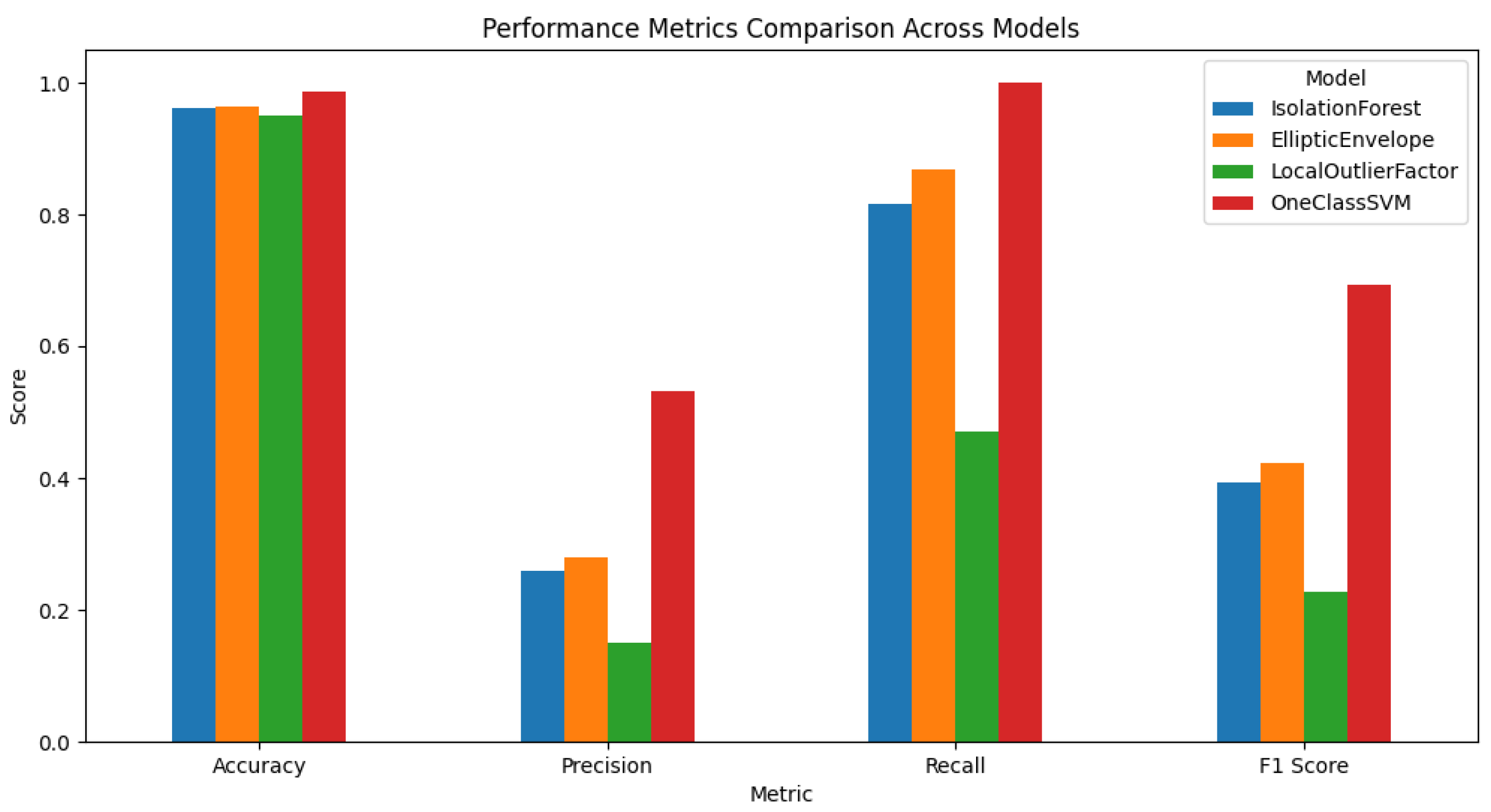
Anomaly detection was accomplished through an ensemble logic, where a data point was deemed anomalous only when 2 or more models deemed it as anomalous. Essentially, this was hedging against the risk of using any model too heavily, while preventing the opportunity to misclassify the data point as an anomalous point. Rare combinations were flagged using a threshold of 2% frequency, whereby the rare combinations were considered potential anomalies. The recorded data for the point would each receive an anomaly score, expressed as the number of models that classified the combination as an anomaly. In the case that two or more models agreed that a data point represented an anomaly, the data point was labelled with ground_truth = -1 (anomaly). Otherwise, the data combination was labelled as normal. This enabled a conservative labelling approach where it was more confident in the labels, and the false positive anomaly rate was also low. Following the labelling of anomalies, the models were finally evaluated on Accuracy, Precision, Recall, and F1-Score, treating anomalies as the positive class. The One-Class SVM was the best of all metrics that were evaluated, with the highest precision, recall, and F1-Score. This demonstrated to be the best model at detecting rare, potentially dangerous combinations, while having the least number of false positives. The Elliptic Envelope and Isolation Forest were very close behind. Local Outlier Factor was shown to be the worst model at correctly identifying true anomalies.
Figure 6.
Performance Comparison Bar Plot.
A separate numeric output (Figure ??) identifies the One-Class SVM as having a low F1 score, and however the bar chart shows One-Class SVM performing the best. This contradiction often occurs when the two sets of results were produced under different scenarios, or with different labeling rules, for example:
- Different Scenarios or Datasets Synthetic vs Real Data - the numeric results might have been produced in a grid search with synthetic anomalies where 5% of the data points have been flipped, while the bar chart may have used the final real dataset or a different version of an existing dataset with labels that were differential.
- Different Labeling Rules GroundTruth Logic - the bar chart may have been produced from a more stringent methodology (for instance, if it required that at least two models agreed on an anomaly) while the numeric F1 score was computed with respect to synthetic labels. These divergences result in different classifications and therefore different performance number. So, the bar chart represents one specific labeling or data scenario where One-Class SVM is the best, with the separate numeric printout coming from another scenario (or as a result of a different labeling approach), which results in a different finding for One-Class SVM.
Clustering
Evaluation of Models
This section discusses the evaluation of Clustering models in terms of metrics. The metrics used in this evaluation are as follows:
Table 4.
Metrics used in evaluating the clustering models.
| Metric | Which one is better |
| Silhouette Score | Measures how well each point fits in its cluster. The Higher the Better |
| Davies-Bouldin Index | Means Separation of Clusters. The Lower the Better |
| Calinski-Harasbasz Index (not for HDBSCAN) | Measures Cluster Variance. Higher is Better |
| Mean Intra-Cluster Distance (HDBSCAN only) | Measures Compactness between clusters |
The evaluation of all 3 models can be summarized in table format as follows:
Table 5.
Results of evaluation of the three models in terms of aforementioned metrics.
| Metric | K-Means (K=4) | K-Means (K=5) | DBSCAN (Best) | HDBSCAN |
| Silhouette Score | 0.5267 | 0.5649 | 0.2439 | 0.8983 |
| Davies-Bouldin Index | 0.7013 | 0.6512 | 0.4893 | 0.3650 |
| Calinski-Harabasz Score | 13252.17 | 12801.27 | 106.58 | N/A |
| Mean Intra-Cluster Distance | N/A | N/A | N/A | 0.0505 |
Evaluation of K-Means Clustering
The previous implementation section discussed the way the model for K-Means clustering was implemented. Now it is time to evaluate the results of the implementation.
The Elbow method, as explained earlier in the implementation, gave k = 4 and k = 5 as possible candidates for the optimal number of clusters.The above-mentioned code compares the two values k = 4 and k = 5 versus the Silhouette Score, Davies-Bouldin Index, and Calinski-Harabasz Score. Testing is done to check on these values as the Elbow method is not 100% accurate. The interpretation of the above results is as follows:
- Silhouette Score: better for k = 5
- Davies-Bouldin Index: better for k = 5
- Calinski-Harabasz Score: better for k = 4
Hence, it can be seen from the above results that the Calinski-Harabasz Score is better for k = 4 with a score of 13252.169174 whereas Davies-Bouldin Index and Silhouette Score are better for k = 5. There is a trade-off here, and the better choice is k = 5 since as per the above it is better than k = 4 for the former metrics, as well as providing better inter-cluster separation than k =4. Best conclusions can, therefore, be made that k = 5 is an optimal value of k.
Evaluation of DBSCAN Clustering
The implementation of DBSCAN Clustering has been discussed earlier under the (Implementation) section. This section evaluates the results of that implementation. As discussed earlier the Elbow method graph showed that the optimal ‘eps’ value lay somewhere between 0.4 and 0.5. As a result, the values of 0.4, 0.45, and 0.5 each were tried with combinations of min_samples_values of 10, 12, and 15 to find the optimal ‘eps’ and the output of the code (discussed in Implementation section) revealed that 0.4 was in fact the optimal ‘eps’ value. We can evaluate these results as follows:
- Silhouette Score (0.2439) is significantly lower than K-Means or HDBSCAN, indicating less defined clusters.
- Davies-Bouldin Index (0.4893) is lower than K-Means, meaning clusters are more distinct, but the result is still suboptimal.
- Calinski-Harabasz Score (106.58) is significantly worse than K-Means, highlighting a lack of clear structure in clusters.
- Key Strength: Can detect noise and outliers, which other methods struggle with.
From this we can conclude that ‘eps’ = 0.4 is the optimal ‘eps’ value for the model.
3.3.1.3. Evaluation of HDBSCAN Clustering
The implementation of HDBSCAN Clustering has been discussed earlier under the (Implementation) section. We can evaluate the results as follows:
- Silhouette Score (0.8983) is the highest, meaning the clusters are extremely well-defined.
- Davies-Bouldin Index (0.3650) is the lowest, confirming that clusters are well-separated.
- Mean Intra-Cluster Distance (0.0505) suggests tight, compact clusters.
- Conclusion: HDBSCAN outperforms both K-Means and DBSCAN in terms of overall quality of clustering.
We can conclude from these observations that the best model is HDBSCAN for clustering as it outperforms both K-Means and DBSCAN when it comes to overall clustering quality.
Validation of Models
This section discusses the validation of models used for clustering. Validation is needed to ensure the model runs as intended and does not face errors and provides consistent results. To measure how consistent the results are over multiple runs, two metrics needed to be computed namely Adjusted Rand Index (ARI) and Normalized Mutual Information (NMI).
Data Visualization and Interpretation
This section mentions all the visualizations created by the models and then interprets their meaning (i.e. discusses what they mean, what trends and patterns they indicate, etc)
Classification
Confusion matrices, ROC and Precision-Recall curves were used to visualize the classification results.
Confusion Matrices
The confusion matrices provide a visualization of each model’s classification performance, highlighting how well they distinguish between opioid-related and non-opioid-related cases. By analyzing these matrices, we can assess key trends such as true positives (TP), false positives (FP), false negatives (FN), and true negatives (TN) across both the base and manually tuned models.
The base and manually tuned models were chosen due to the base models being the worst performing (due to overfitting) and manually tuned models being the best performing which can be used to highlight the more apparent comparisons.
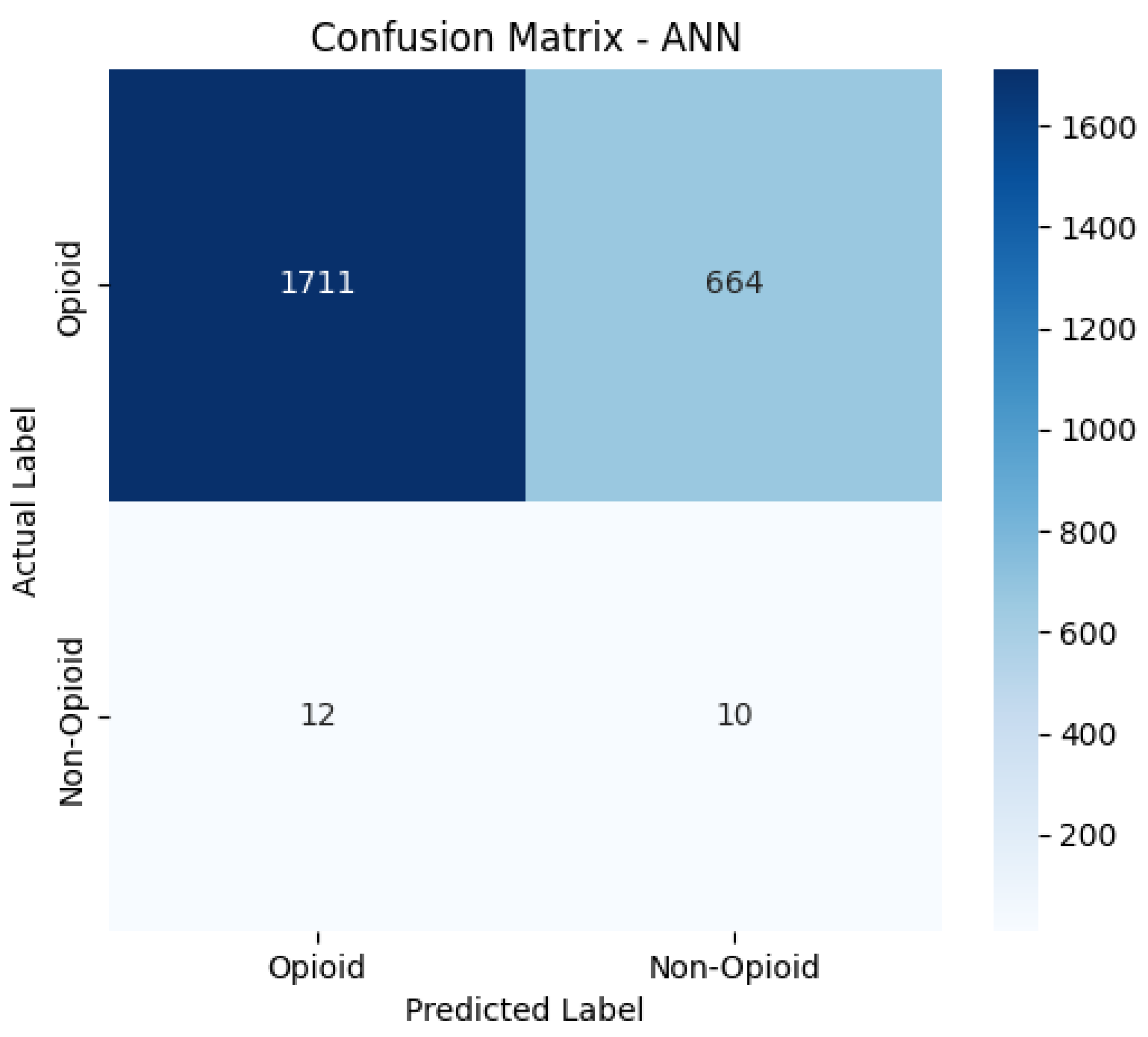
Base Model Performance
The base model performances all show exceptionally high true positives and false positives, meaning they classify nearly all opioid-related cases correctly. However, this comes at the cost of many false positives, leading to poor precision. It is apparent that the base models are biased towards the majority class and are mostly predicting the majority class.
Figure 7.
Confusion Matrix for Random Forest (base).
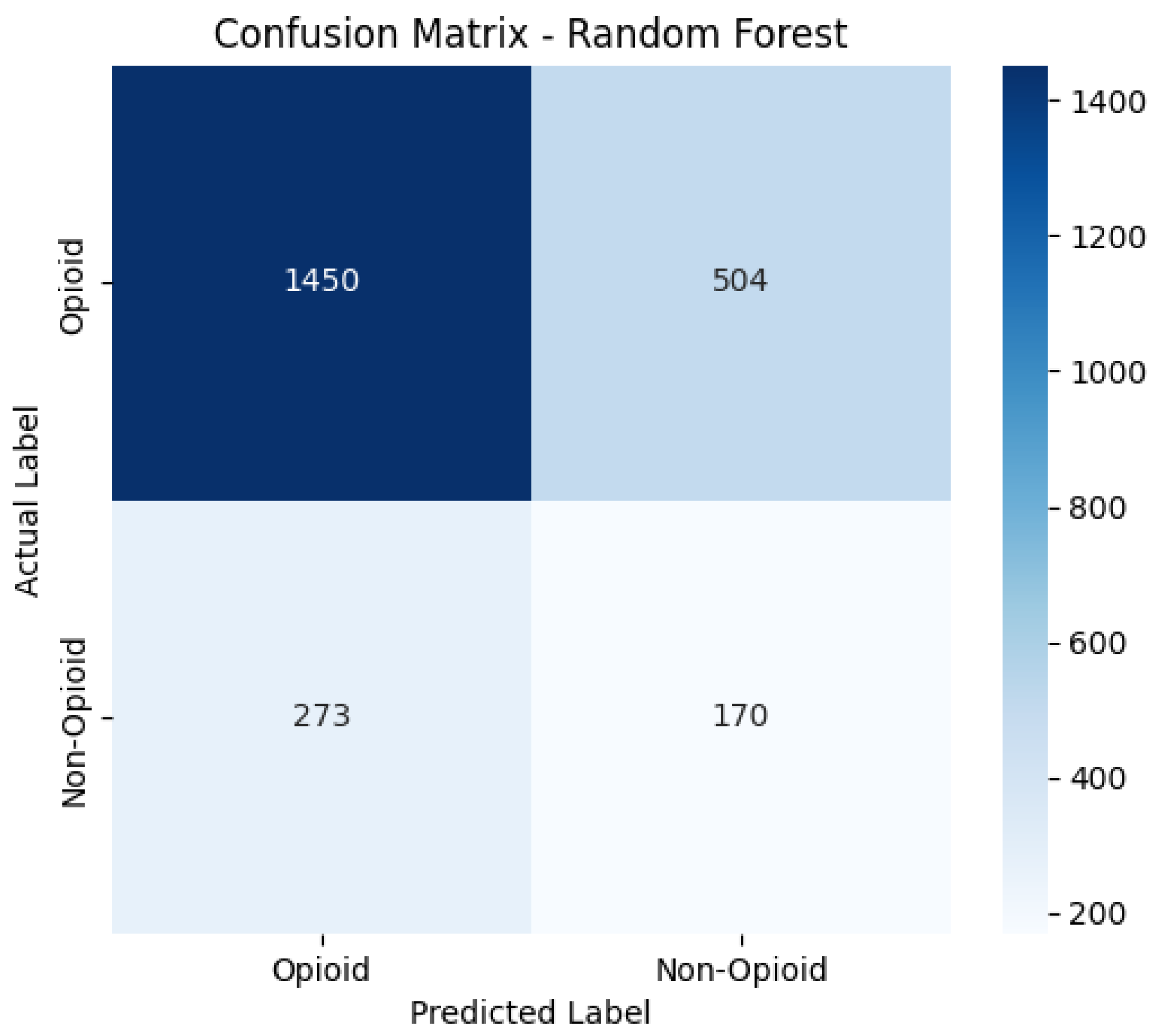
Figure 8.
Confusion Matrix for XGBoost (base).
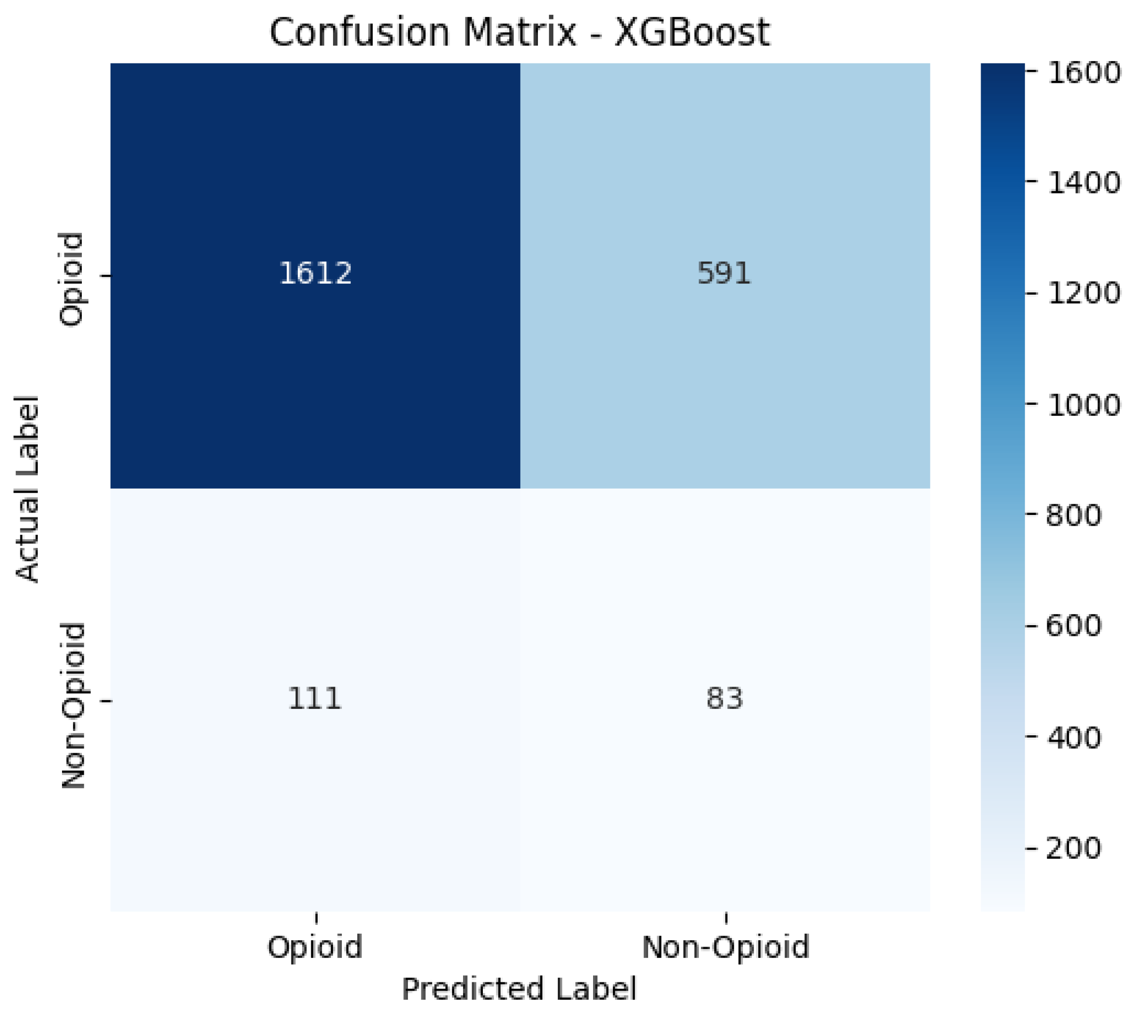
Figure 9.
Confusion Matrix for Logistic Regression (base).
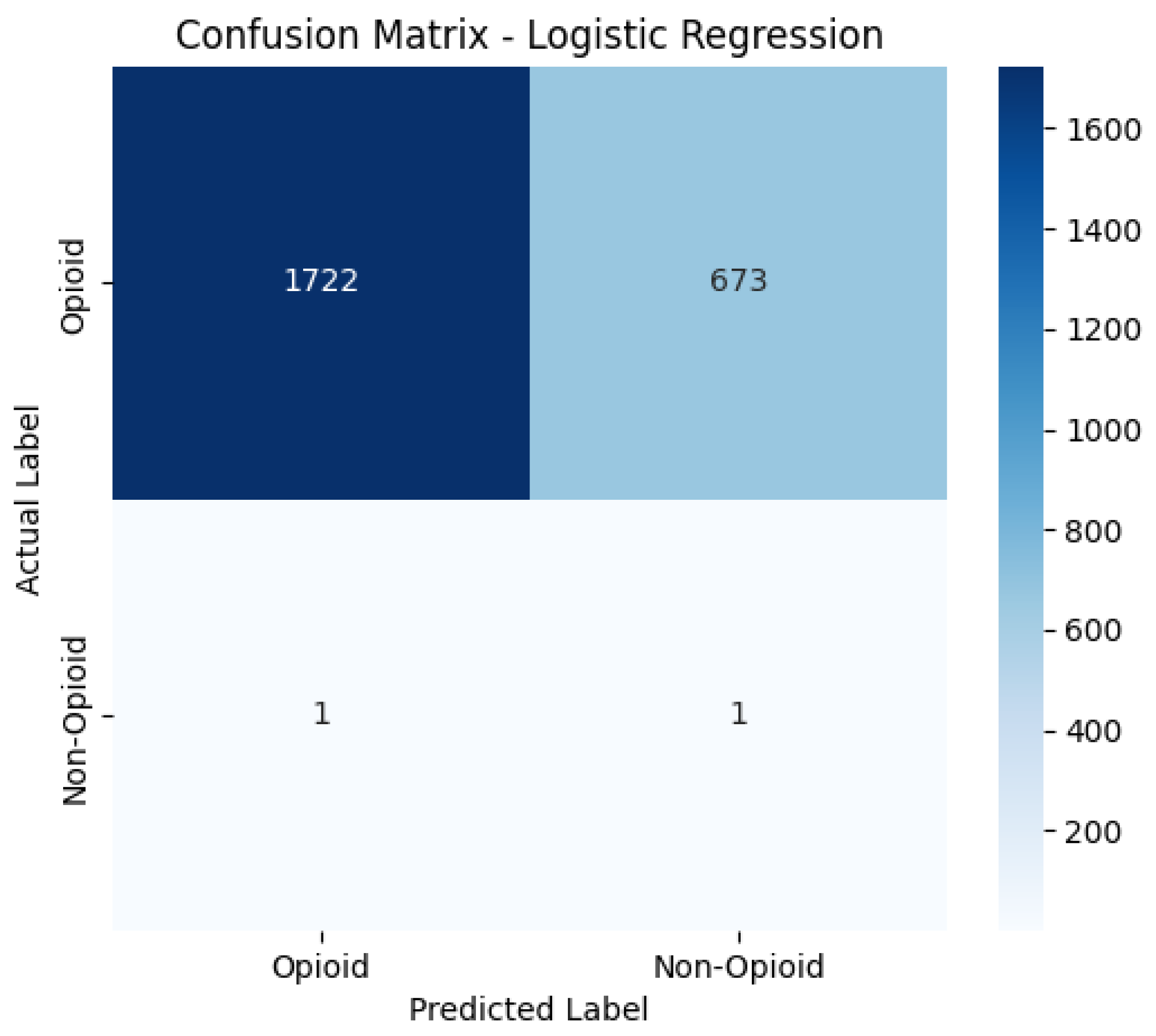
Figure 10.
Confusion Matrix for SVM (base).
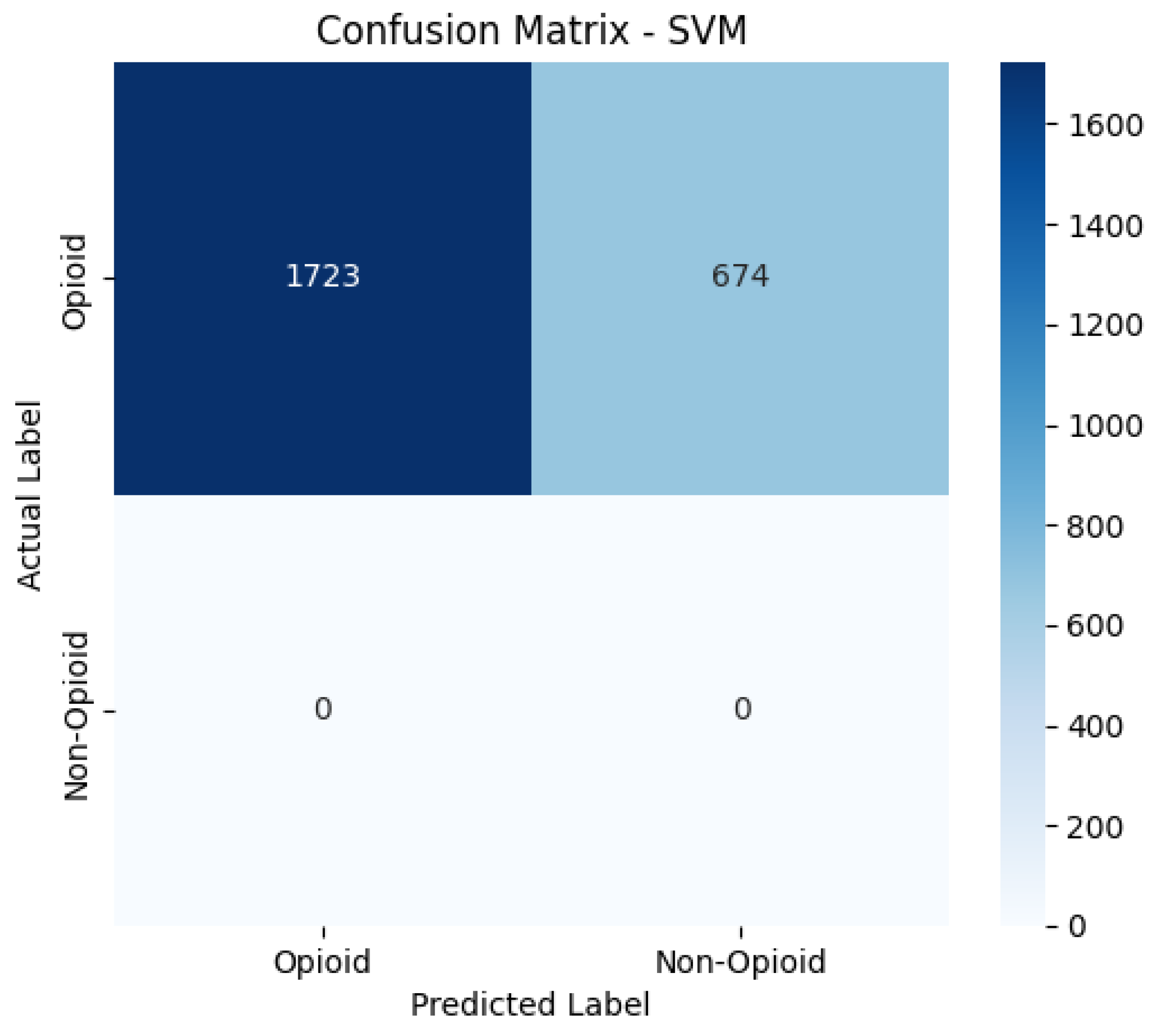
Figure 11.
Confusion Matrix for ANN (base).
4.1.2. ROC Curve Analysis
The Receiver Operating Characteristic (ROC) curves evaluate the trade-off between True Positive Rate (TPR) and False Positive Rate (FPR) at various thresholds. The dashed diagonal reference line represents a random classifier (a model making totally random predictions). Ideally, a good classifier should curve away from this line towards the top-left corner.
Figure 12.
Base ROC Curve.
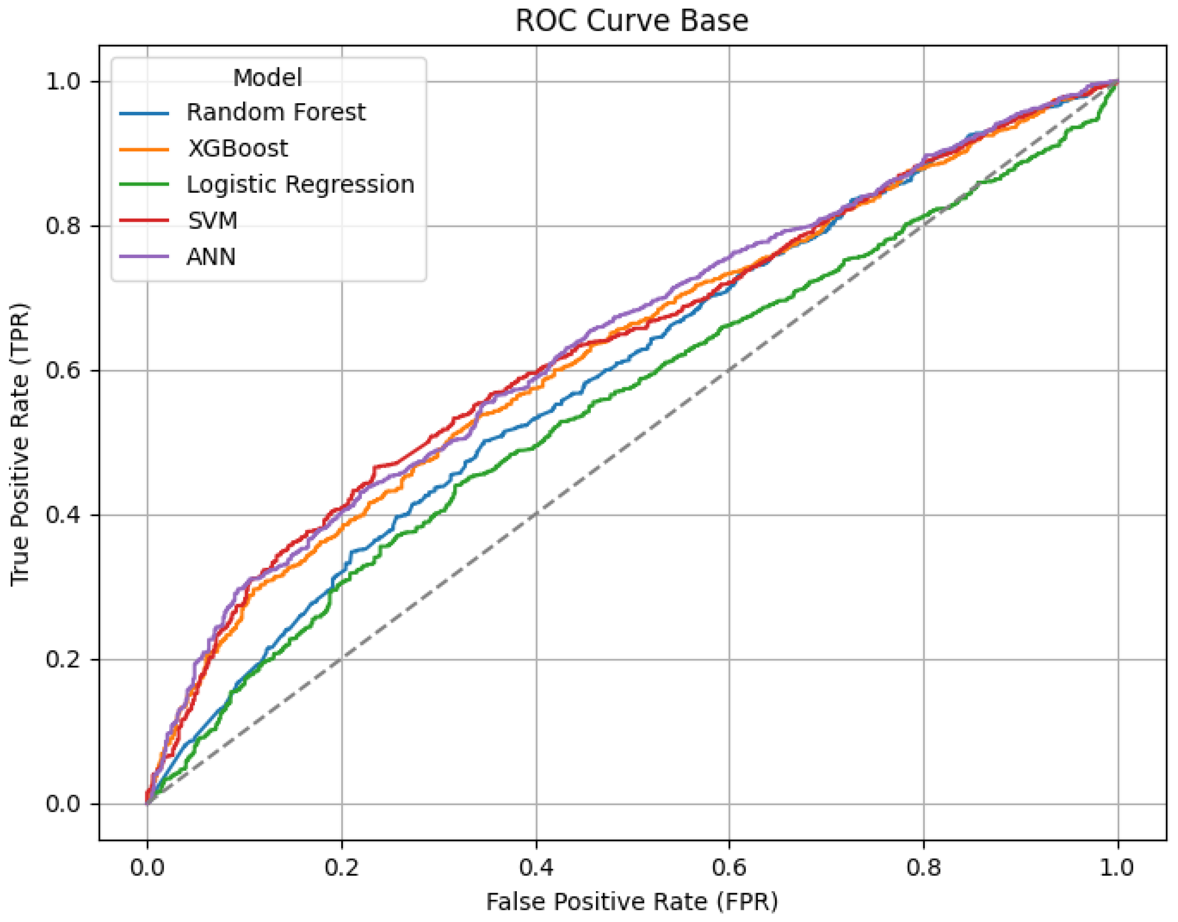
XGBoost and SVM show the highest lift over the random classifier line, showing better discrimination ability. Random Forest also shows a reasonable curve about as steep as XGBoost. ANN performs moderately while Logistic Regression performs the worst, with curves close to the diagonal. Moreover, Logistic Regression appears closest to random, as it struggles to distinguish between opioid and non-opioid cases effectively. The ROC curve for the manually tuned models is more distinctly separated from the diagonal dashed line as they curve more towards the top-left corner as shown below.
Figure 13.
ROC Curve for Tuned Models.
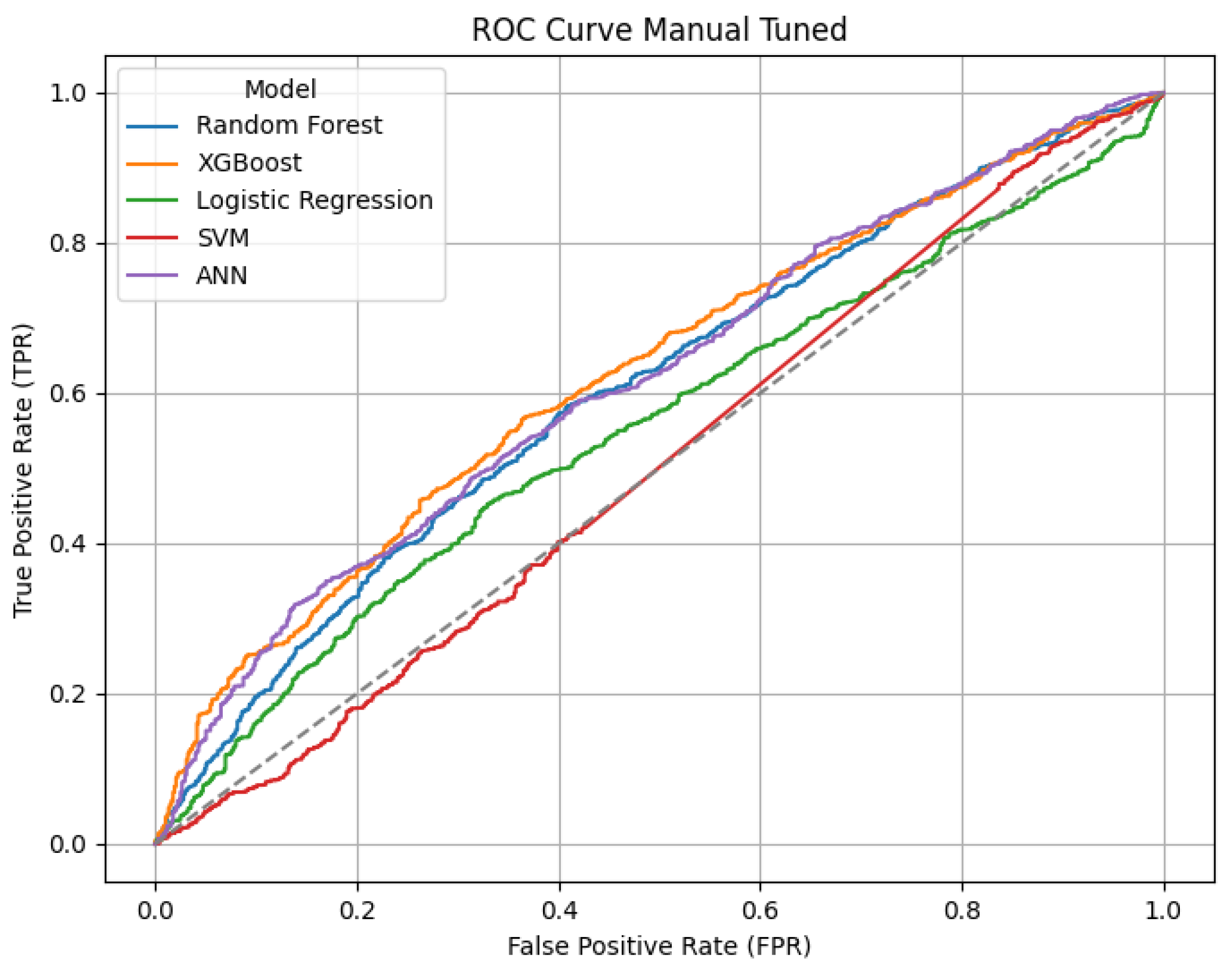
XGBoost and Random Forest show consistent improvements while SVM and Logistic Regression remain weaker classifiers, with SVM now performing almost randomly. XGBoost and Random Forest maintain the farthest distance from the random classifier line, indicating that they are the best at distinguishing between opioid and non-opioid cases. Random Forest has also improved, achieving a better trade-off between TPR and FPR. Most models now follow a stable curve.
Precision-Recall Curve Analysis
The below Precision-Recall (PR) curve visualizes the performance of the base models before dataset balancing and hyperparameter tuning.
Figure 14.
Base PR Curves.
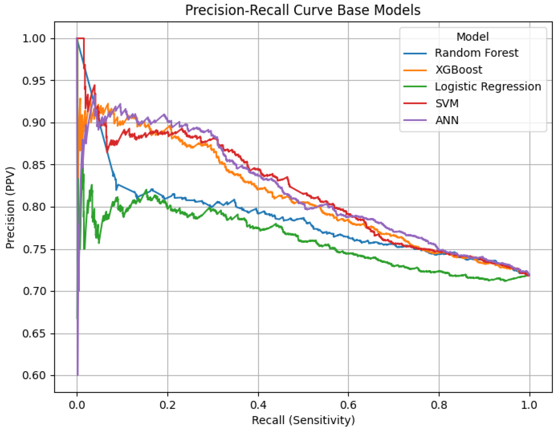
As recall increases, precision tends to decrease, which is expected. XGBoost, Random Forest and XGBoost maintain higher precision even at lower recall values, meaning they are better at identifying opioid cases correctly while avoiding false positives. Similar to the previous visualizations, Logistic Regression consistently performs the worst, staying significantly below the other models showing extreme instability.
Unlike the ROC curve, which evaluates performance across all classification thresholds, the PR curve is more informative for imbalanced datasets like this one. The gap between the models is much clearer in this graph, with XGBoost and Random Forest demonstrating superior precision-recall trade-offs. The model’s stability is apparent due to the smoother curves, meaning the precision does not drop too sharply with increasing recall. The following Precision-Recall (PR) curve shows the performance of the manually tuned models trained on the sampled dataset.
Figure 15.
PR Curves for Tuned Models.
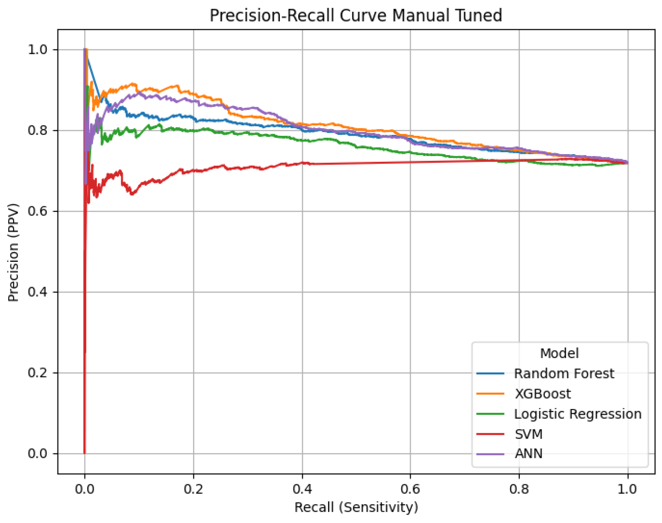
The precision at lower recall values have stabilized compared to base models. XGBoost maintains the highest precision over a wide recall range. Random Forest shows improved stability, though slightly behind XGBoost. ANN remains in an intermediate position while SVM performs the worst despite tuning and balancing. Random Forest and XGBoost demonstrate the most consistent performance across all recall values. ANN follows a smooth declining trend, showing better generalization. SVM and Logistic Regression perform consistently but show poor results as the curves are lower.Compared to the base models, the manually tuned models maintain higher precision across all recall levels. The improved precision-recall trade-off across all models show that dataset balancing and tuning significantly enhanced performance. The optimal model selection should prioritize models that maintain high recall while mitigating false positives. Overall, these improvements highlight the effectiveness of SMOTE and hyperparameter tuning.
Anomaly Detection
Isolation Forest: Opioid and Depressant Combinations
The Isolation Forest algorithm detected several rare and high-risk combinations, with the first being heroin, fentanyl, fentanyl analogue, benzodiazepine, and methadone in about 14 cases. Such a cocktail drastically increases the risk of overdose due to the aggregate CNS depressant effect. Another noted combination was oxycodone, oxymorphone, and ethanol in 10 cases, where mixing of the opioids and alcohol produces a grievous respiratory hazard. One pattern that emerged from this model was the mixing of opioids with benzodiazepines or ethanol, often involving fentanyl analogues-warranting the evolution of overdose threats.
Elliptic Envelope: Prescription Opioid Abuse Patterns
According to the elliptical envelope methodology, uncommon and hence dangerous combinations pointed to 25 cases involving oxycodone, oxymorphone, and benzodiazepine, giving insights into problematic prescription opioid misuse with tranquilizers. The second most infrequent combination of oxycodone and oxymorphone (24 cases) illustrates their conjoint use as a high-power and overdose-risk situation. Other observations, such as the frequent appearance of benzodiazepine with opiate_nos and ethanol with opioids, reveal so-to-say-safe dangerous combinations. And perhaps some stimulant-involved combinations-e.g., meth cuts the clinical picture with their opposing pharmacologic effects.
Local Outlier Factor: Speedballs and Unregulated Substances
The Local Outlier Factor model pointed out cocaine with gabapentin (12 cases) and heroin, cocaine, fentanyl, xylazine (10 cases) as especially concerning. These combinations paint a visage of dangerous polydrug use that involves both stimulants and opioids (alias speedballs). The presence of xylazine, a veterinary sedative being found increasingly in street drugs, signals a move toward cheap and unregulated experimentation.
One-Class SVM: High-Risk Depressant Combinations
One-Class SVM identified oxycodone, oxymorphone, ethanol, and benzodiazepine (6+ cases) as a leading rare but deadly combination, followed by heroin, fentanyl, fentanyl analogue, ethanol, benzodazepine, and methadone (5 cases). These combinations reflect a synergy of multiple potent opioids with alcohol and sedatives, greatly amplifying overdose risks. Notably, this model pinpointed the mixed use of prescribed and illicit opioids with depressants, which concurs with new overdose crisis patterns. These findings justify the need for interventions for combined opioid-benzodiazepine or opioid-alcohol use.
General Observations Across All Models
Across the four models, there were several recurring themes—most prominently the combination of opioids with benzodiazepines or ethanol, a long-known driver of fatal overdoses. The fact that fentanyl analogues and xylazine were present also shows the growing role of novel and unregulated drugs in overdose cases. Top 10 lists differed across the models based on their detection rationale, with some picking up more opioid-depressant combinations and others picking up stimulant-opioid combinations. These results collectively underscore the urgent need for targeted surveillance and interventions against the complex and fatal phenomenon of polydrug abuse.
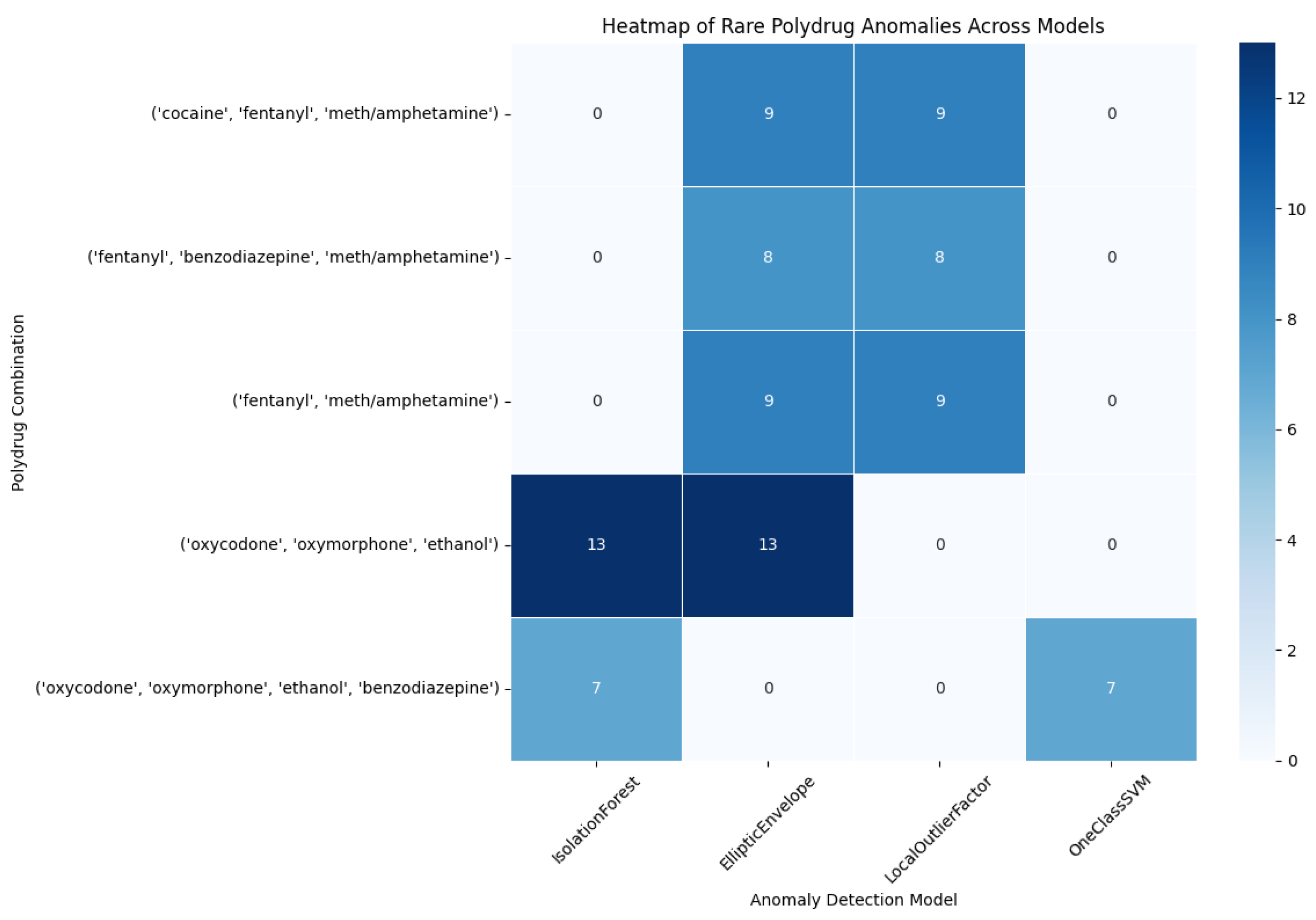
4.2.2. Heatmap
This heatmap shows the frequency of flagging of each of several infrequent polydrug combinations by four anomaly detection algorithms: IsolationForest, EllipticEnvelope, LocalOutlierFactor and OneClassSVM. The rows represent a particular polydrug combination, for instance, ('cocaine', 'fentanyl', meth/amphetamine') while the columns represent one of the four models.
- The scale of colors starts from the light color for fewer flagged cases to the dark color for more flagged cases.
- The count of how many times that combination was labeled as anomalous by the respective model is shown in the values present inside the cells.
These polydrug combinations are referred to as ‘rare’ since they are not common in the dataset but are dangerous (for example, risk of overdose).
Figure 16.
Heatmap Rare Polydrug Anomalies Across Models.
Anomaly Detection Comparison
This bar plot illustrates the predictions of the four anomaly detection models based on the normal labeled dataset (label = “1”) and anomalous labeled dataset (label = “-1”). The classification labels are on the x-axis, and the frequency (or number of data points) are shown on the y-axis.
Figure 17.
Comparison of Normal (1) vs. Anomalous (-1) Classifications by Four Anomaly Detection Models.
Figure 17.
Comparison of Normal (1) vs. Anomalous (-1) Classifications by Four Anomaly Detection Models.
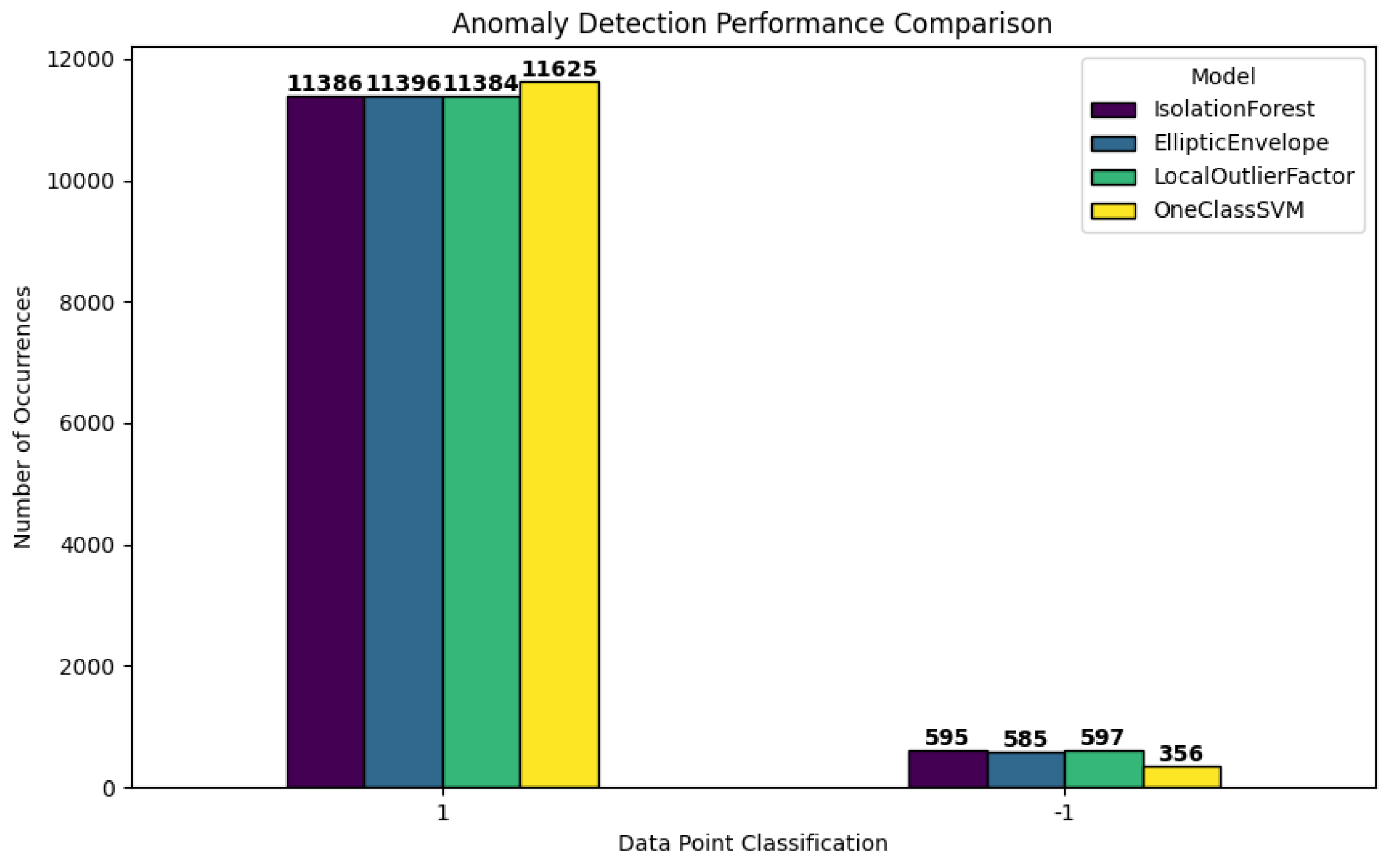
Normal Class (1)- All models have correctly detected most of the records as normal from the highest bars of approximately 11,000 each for the normal class. This is due to most of the data points being a typical polydrug use pattern that is being expected by the models.
Anomaly Class (-1) - Each model has flagged different amounts of points as outliers on the right-hand side of the figure by the smaller bars which were 595 (IsolationForest) to 356 (OneClassSVM). The reason is that each algorithm has its own way of explaining what is unusual in the data based on the algorithms internal working and the parameters.
In general, the chart shows that all models agree that there were approximately 500 anomalies in the data set, but all models’ bands are quite small compared to the normal class; however, the number of anomalies changes depending on the model.
Drug Presence in Normal Vs Anomalous Cases
This bar graph Figure 18 provides a comparison of average prevalence of each drug occurring (in normal cases (represented with blue bars) and anomalous cases (represented with orange bars)). The horizontal axis identifies specific drugs, and the vertical axis demonstrates average prevalence -- the frequency of occurrence of the identified substance in each group's records -- either normal or anomalous. A few patterns observed:
Clustering
This section describes the visualizations created based on the Clustering models and interprets their significance as shown in Figure 19.
K-Means Scatter Plots
The two graphs Figure 19 and Figure 20 above present K-Means clustering of geographical data (‘death_latitude’ and ‘death_longitude’ columns from dataset) done using two separate K values of 4 and 5.
When K = 5, there are 5 clusters represented by a distinct colour (the points are all of 5 distinct colours each colour representing a cluster). The clustering seems to be well oriented as it exemplifies the spatial pattern. The points inside some of the clusters are more tightly packed, while those in other clusters are more dispersed, which means that K = 5 aims to segment the data into a more detailed subdivision. However, when K = 4, there are 4 clusters each represented with a distinct colour (the points are all of 4 distinct colours each colour representing a cluster). The fewer number of clusters suggest that the data points have been grouped in a more general way than in the K = 5. Some of the clusters were independent clusters in the K = 5 have now merged indicating that fewer clusters may suggest less distinct segmentation. the structure of the clusters is still present but there is more generalization compared to the k = 5 scenario. The K=5 clustering offers a finer granularity thus having more specific and smaller groups in comparison to K= 4. The K=4 clustering had fewer groups and the groups are larger; this may be beneficial if broad segmentation is desired, but not if specific segments are desired. The decision between K=4 and K=5 is dependent on the detail desired for the analysis. If the researcher wishes to better distinguish the groups, K=5 is the better choice whereas K=4 if the study is requesting generalized segmentations.
This graph Figure 21 shows Optimized DBSCAN Clustering of geographical data (‘death_latitude’ and ‘death_longitude’ columns from the dataset) with ‘esp’ = 0.4 and min_samples = 10 parameters.
The points in dark blue are labelled –1 (i.e. noise). They are non-core points that are not part of any cluster and as you can see there are hosue noise points in the graph. There are a small number of clusters (yellow, green, purple, teal), which have been identified in areas where the points were at higher density. These clusters are small indicating that there are only a few areas of sufficient point density to be grouped. Epsilon (eps=0.4), is used to determine the range of neighbours where a point can have a neighbouring point (to cluster), a smaller value indicates that only very near points could be considered as part of a cluster. At the same time, min_samples=10, means that, to form a cluster, there must be a minimum of 10 points within that radius, this does limit small random groups, but runs the risk of leaving a lot of points un-clustered. The colour bar (on the right) shows that most points are labelled noise (-1) and only a few small dispersed (scattered) clusters were identified, suggesting that there are limited areas within the data-set to demonstrate dense neighbourhoods.
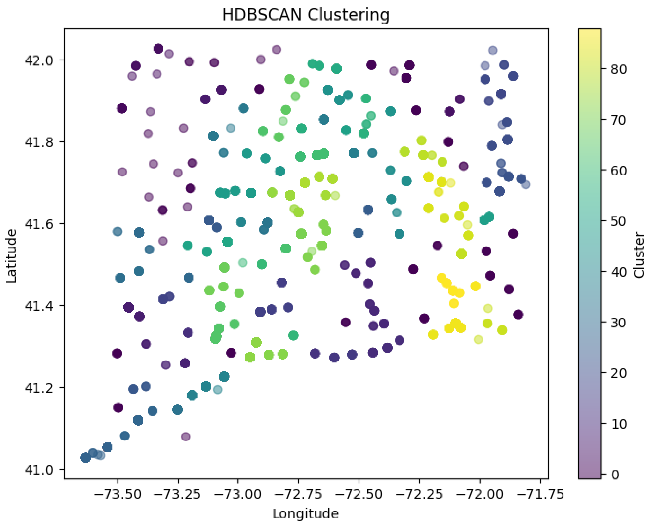
This plot Figure 22 shows HDBSCAN Clustering applied to spatial data (the columns in the data set labelled 'death_latitude' and 'death_longitude').
The colours correspond to clusters. The colour scale on the right indicates quite a few unique clusters (with more than 80 labelled). This means fine-grained cluster detection was possible. The dark-green cluster on the far right has a majority of its points assigned to it while the yellow, green and teal cluster have larger concentrations of points. The far-left regions of purple and blue indicated more sparse assignments. The implied clustering structure suggests a density-based grouping that suggests clustering is oriented on where points are dense rather than strictly groups to partitioning data. HDBSCAN does not require each point to be assigned to a cluster so there are a lot of low-desnity regions and noise points both as well as cluster points. And because HDBSCAN is a density-based clustering algorithm, it works to create clusters for where data points are already densely grouped naturally as opposed to arbitrarily partitioning space. This suggests a lot of confidence for the identification of complex spatial multi-patterns and structural hierarchy.
Conclusions
This study examined the use of data mining techniques, classification, clustering, and anomaly detection, to investigate accidental deaths related to drugs and learn meaningful lessons for the purpose of predictive modeling. The application of the various study techniques guided us to identify areas of high-risk, dangerous combinations of substances, and demographic factors associated with opioid use.
The major results of the study demonstrated the power of many machine learning techniques for finding patterns in the dataset: Classification models robustly predicted opioid involvement in an overdose, with Random Forest and XGBoost being the best-performing models, as these models must provide a balance of precision and recall for use in practice for an overdose risk decision support model. Anomaly detection models were able to identify rare, sometimes lethal, polydrug combinations and may serve as an early warning sign of new overdoses in a geographical area. Clustering models (K-Means, DBSCAN, HDBSCAN) segmented geographical location based on overdose incidence rates. HDBSCAN was the most robust clustering model because it was able to provide useful detail on high incidence-risk areas that may be targeted later for intervention.
These findings provide a data-driven approach to overdose prevention by highlighting the most vulnerable populations and geographical hotspots where intervention strategies—such as law enforcement measures, public awareness campaigns, and healthcare resource allocation—can be optimized.
Challenges and Limitations
Although this research was successful, it was limited in a few ways:
The dataset lacked socioeconomic and healthcare variables, limiting the ability to fully explain overdose trends. Future research could include socioeconomic variables (for example income levels and healthcare access) as well as law enforcement presence, which may make the predictions more accurate. There were challenges with the models' tunings, particularly with DBSCAN and HDBSCAN that needed careful selection of hyperparameters to produce good clustering models. Also, the classification models had impacts on the predictions due to data class imbalance and whether or not I was able to use techniques like SMOTE or SMOTE-Tomek resampling which may make models more fair and reliable.
Future Recommendations
To improve the accuracy and usability of our results, future research can include more socioeconomic data ( demographic, economic, etc.) so that overdose patterns can be interpreted more clearly, allowing policymakers to make better-targeted decisions. Also, developing an automated for model optimization using Bayesian Optimization or Genetic Algorithms can improve clustering because the need for manually tuning hyperparameters would be diminished. Creating real-time risk predictions through classification or anomaly detection to issue alerts for high-risk cases could allow those in healthcare and law enforcement to intervene earlier. Lastly, exploring advanced deep learning approach (e.g. Long Short-Term Memory networks, Convolutional Neural Networks) could help improve predictive accuracy of prescription opioid classification models and provide richer information regarding overdose trends that could help decision-making.
References
- Agyemang, E. F. (2024). Anomaly detection using unsupervised machine learning algorithms: A simulation study. Scientific African, e02386–e02386. [CrossRef]
- Arora, S., Hu, W., & Kothari, P. K. (2018). An Analysis of the t-SNE Algorithm for Data Visualization. PMLR, 1455–1462. https://proceedings.mlr.press/v75/arora18a.html.
- CDC. (2024). Understanding the opioid overdose epidemic. Overdose Prevention. https://www.cdc.gov/overdose-prevention/about/understanding-the-opioid-overdose-epidemic.html.
- Chandola, V., Banerjee, A., & Kumar, V. (2009). Anomaly Detection: A Survey. ACM Computing Surveys, 41(3), 1–58. [CrossRef]
- Com, L., & Hinton, G. (2008). Visualizing Data using t-SNE Laurens van der Maaten. Journal of Machine Learning Research, 9, 2579–2605. https://www.jmlr.org/papers/volume9/vandermaaten08a/vandermaaten08a.pdf.
- Durgesh Samariya, Ma, J., Aryal, S., & Zhao, X. (2023). Detection and explanation of anomalies in healthcare data. 11(1). [CrossRef]
- G.Malarselvi. (2024). A Multifaceted Approach for Enhancing Anomaly Detection in Industrial Systems with Adaptive Synthetic Sampling and Machine Learning Evaluation. Journal of Electrical Systems, 20(5s), 2124–2131. [CrossRef]
- https://www.facebook.com/thoughtcodotcom. (2019). Is Springfield the Most Common Place Name in the United States? ThoughtCo. https://www.thoughtco.com/place-name-in-all-fifty-states-1435154?utm_.
- in. (2015, March 26). Optimal number of bins in histogram by the Freedman–Diaconis rule: difference between theoretical rate and actual number. Cross Validated. https://stats.stackexchange.com/questions/143438/optimal-number-of-bins-in-histogram-by-the-freedman-diaconis-rule-difference-be.
- Johns Hopkins Medicine. (2022, October 19). Opioids. Www.hopkinsmedicine.org; John Hopkins Medicine. https://www.hopkinsmedicine.org/health/treatment-tests-and-therapies/opioids.
- Krawiec, P., Junge, M., & Hesselbach, J. (2021). Comparison and Adaptation of Two Strategies for Anomaly Detection in Load Profiles Based on Methods from the Fields of Machine Learning and Statistics. Open Journal of Energy Efficiency, 10(2), 37–49. [CrossRef]
- Matharaarachchi, S., Domaratzki, M., & Muthukumarana, S. (2024). Enhancing SMOTE for imbalanced data with abnormal minority instances. Machine Learning with Applications, 18, 100597. [CrossRef]
- Naarayanan, B., Franklin, C., Gouvtham, N., & Femi, S. (n.d.). Comparing the Performance of Anomaly Detection Algorithms. https://www.ijert.org/research/comparing-the-performance-of-anomaly-detection-algorithms-IJERTV9IS070532.pdf.
- Nguyen, A., Wang, J., Holland, K. M., Ehlman, D. C., Welder, L. E., Miller, K. D., & Stone, D. M. (2024). Trends in Drug Overdose Deaths by Intent and Drug Categories, United States, 1999‒2022. American Journal of Public Health, 114(10), 1081–1085. [CrossRef]
- Saeed, S. (2019). Analysis of software development methodologies. IJCDS. Scopus; Publish.
- Saeed, S. (2019). The serverless architecture: Current trends and open issues moving legacy applications. IJCDS. Scopus.
- Saeed, S., & Humayun, M. (2019). Disparaging the barriers of journal citation reports (JCR). IJCSNS: International Journal of Computer Science and Network Security, 19(5), 156-175. ISI-Index: 1.5.
- Saeed, S. (2016). Surveillance system concept due to the uses of face recognition application. Journal of Information Communication Technologies and Robotic Applications, 7(1), 17-22.
- Nkugwa Mark William. (2023, October 31). How to Determine Bin Width for a Histogram ( R and Python). Medium. https://nkugwamarkwilliam.medium.com/how-to-determine-bin-width-for-a-histogram-r-and-pyth-653598ab0d1c.
- Sadeq Darrab, Harshitha Allipilli, Ghani, S., Harikrishnan Changaramkulath, Koneru, S., Broneske, D., & Saake, G. (2023). Anomaly Detection Algorithms: Comparative Analysis and Explainability Perspectives. Communications in Computer and Information Science, 90–104. [CrossRef]
- sklearn.metrics.matthews_corrcoef. (n.d.). Scikit-Learn. https://scikit-learn.org/stable/modules/generated/sklearn.metrics.matthews_corrcoef.html.
- Spencer, M. R., Garnett, M. F., & Miniño, A. M. (2024). Drug Overdose Deaths in the United States, 2002–2022. Www.cdc.gov. https://www.cdc.gov/nchs/products/databriefs/db491.htm.
- The Lancet. (2023). Opioid crisis: addiction, overprescription, and Insufficient Primary Prevention. The Lancet Regional Health- Americas, 23(100557), 100557–100557. [CrossRef]
- Wolff, J., Gitukui, S., O’Brien, M., Mital, S., & Noonan, R. K. (2022). The Overdose Response Strategy: Reducing Drug Overdose Deaths Through Strategic Partnership Between Public Health and Public Safety. Journal of Public Health Management and Practice, 28(Supplement 6), S359–S366. [CrossRef]
- World Health Organization. (2023, August 29). Opioid overdose. World Health Organization. https://www.who.int/news-room/fact-sheets/detail/opioid-overdose.
- Jhanjhi, N.Z. (2025). Investigating the Influence of Loss Functions on the Performance and Interpretability of Machine Learning Models. In: Pal, S., Rocha, Á. (eds) Proceedings of 4th International Conference on Mathematical Modeling and Computational Science. ICMMCS 2025. Lecture Notes in Networks and Systems, vol 1399. Springer, Cham. [CrossRef]
- Humayun, M., Khalil, M. I., Almuayqil, S. N., & Jhanjhi, N. Z. (2023). Framework for detecting breast cancer risk presence using deep learning. Electronics, 12(2), 403.
- Gill, S. H., Razzaq, M. A., Ahmad, M., Almansour, F. M., Haq, I. U., Jhanjhi, N. Z., ... & Masud, M. (2022). Security and privacy aspects of cloud computing: a smart campus case study. Intelligent Automation & Soft Computing, 31(1), 117-128.
- Aldughayfiq, B., Ashfaq, F., Jhanjhi, N. Z., & Humayun, M. (2023, April). Yolo-based deep learning model for pressure ulcer detection and classification. In Healthcare (Vol. 11, No. 9, p. 1222). MDPI.
- N. Jhanjhi, "Comparative Analysis of Frequent Pattern Mining Algorithms on Healthcare Data," 2024 IEEE 9th International Conference on Engineering Technologies and Applied Sciences (ICETAS), Bahrain, Bahrain, 2024, pp. 1-10. [CrossRef]
- Ray, S. K., Sirisena, H., & Deka, D. (2013, October). LTE-Advanced handover: An orientation matching-based fast and reliable approach. In 38th annual IEEE conference on local computer networks (pp. 280-283). IEEE.
- Samaras, V., Daskapan, S., Ahmad, R., & Ray, S. K. (2014, November). An enterprise security architecture for accessing SaaS cloud services with BYOD. In 2014 Australasian Telecommunication Networks and Applications Conference (ATNAC) (pp. 129-134). IEEE.
Figure 18.
Average Drug Presence in Normal Versus Anomalous Polydrug Cases.
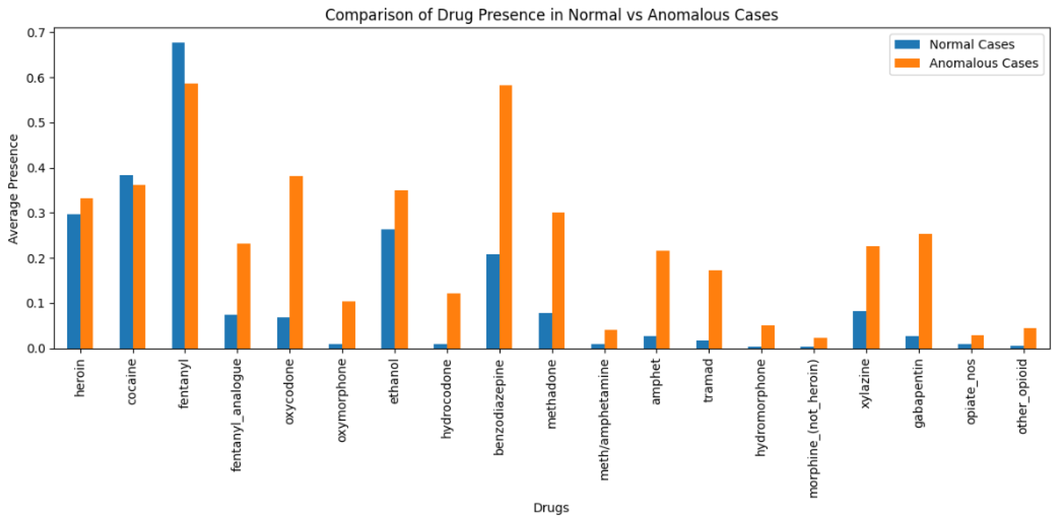
Figure 19.
Scatter Plot for K=4.
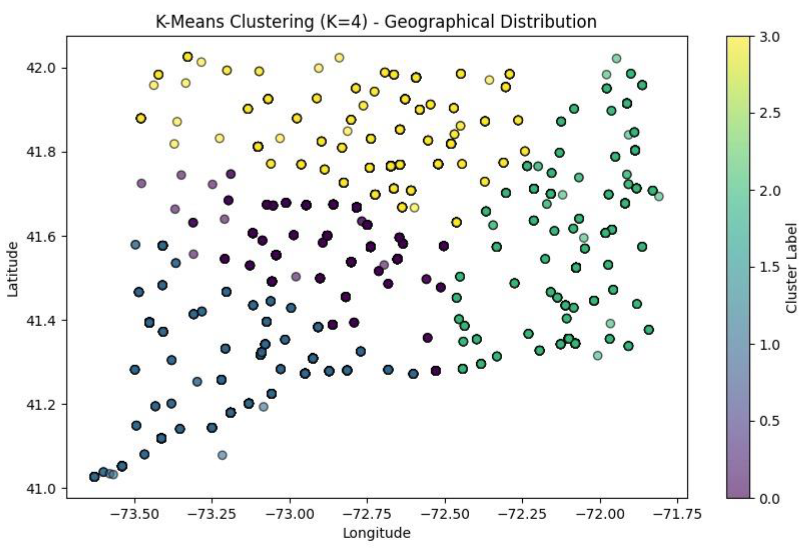
Figure 20.
Scatter Plot for K=5.
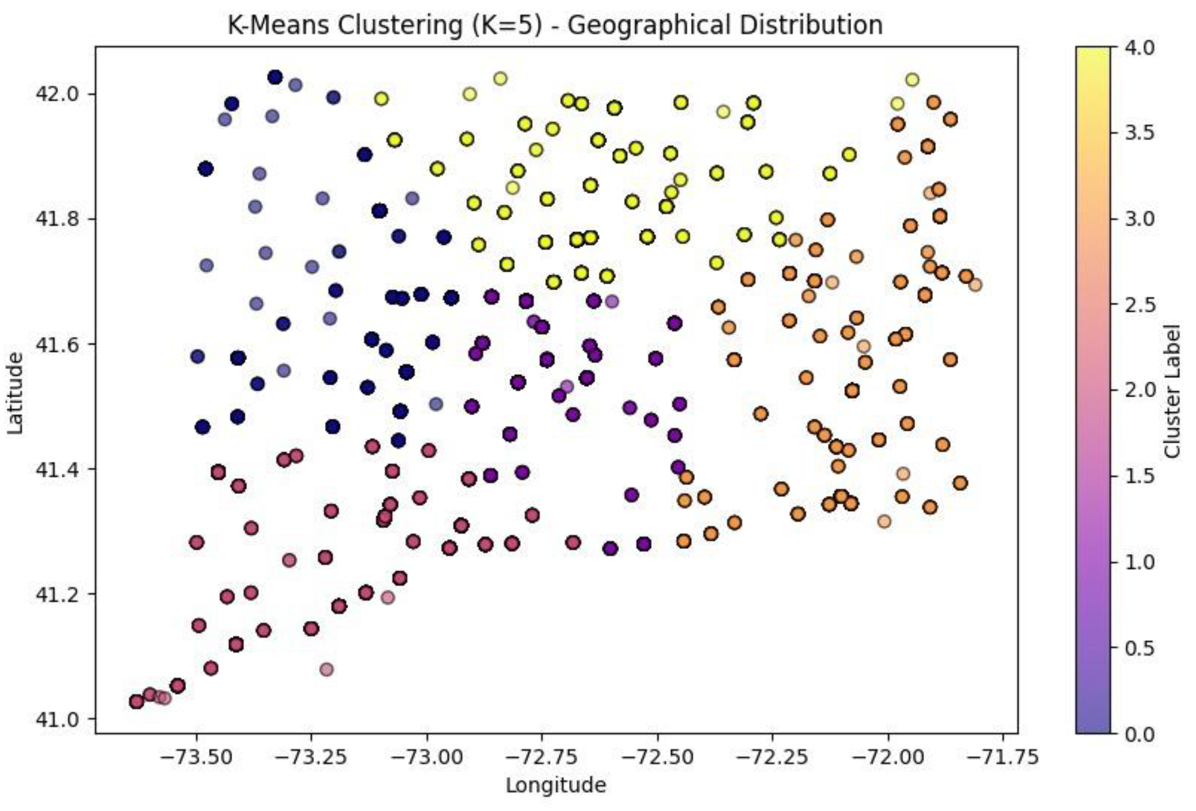
Figure 21.
Scatterplot Optimized DBSCAN Clustering Results.
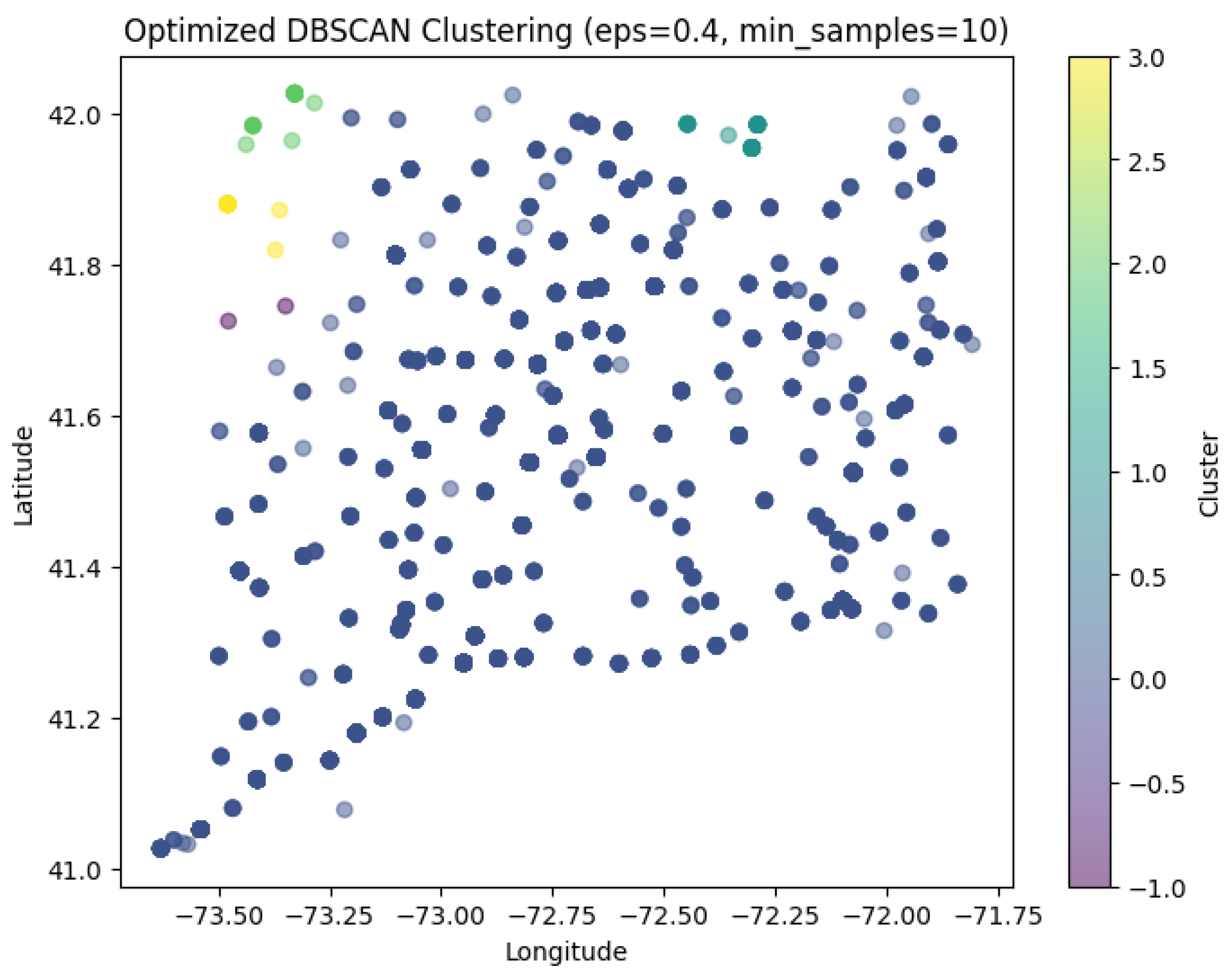
Figure 22.
Scatterplot showing HDBSCAN Clustering Results.
Disclaimer/Publisher’s Note: The statements, opinions and data contained in all publications are solely those of the individual author(s) and contributor(s) and not of MDPI and/or the editor(s). MDPI and/or the editor(s) disclaim responsibility for any injury to people or property resulting from any ideas, methods, instructions or products referred to in the content. |
© 2025 by the authors. Licensee MDPI, Basel, Switzerland. This article is an open access article distributed under the terms and conditions of the Creative Commons Attribution (CC BY) license (http://creativecommons.org/licenses/by/4.0/).
Copyright: This open access article is published under a Creative Commons CC BY 4.0 license, which permit the free download, distribution, and reuse, provided that the author and preprint are cited in any reuse.


