
Submitted:
29 April 2025
Posted:
30 April 2025
You are already at the latest version
Abstract
Recent advances in Artificial Intelligence (AI)-driven wireless communication demand innovative Sixth Generation (6G) solutions, particularly in hospitals where reliability and secure communication are crucial. Visible Light Communication (VLC) leverages existing lighting systems to deliver high data rates while mitigating electromagnetic interference. However, VLC systems in medical settings face fluctuating signal strength and dynamic channel conditions due to patient movement, necessitating advanced optimization techniques. This paper employs a site-specific ray tracing technique in Medical Body Sensor Networks (MBSNs) channel modeling within hospital scenarios to derive channel impulse responses (CIRs) and model path loss (PL) and Root Mean Square (RMS) delay spread in two distinct hospital settings. In the first section, we evaluate Machine Learning (ML)-based adaptive modulation in VLC-enabled MBSNs and introduce a Q-learning technique enabling real-time adaptation without prior environmental knowledge. In the second section, we propose a Long Short Term Memory (LSTM) based approach to estimate PL and RMS delay spread in dynamic hospital environments. The Q-learning method consistently achieved the target symbol error rate (SER), though spectral efficiency (SE) was sometimes lower than optimal due to quantization limits and a cautious approach near the SER threshold. For LSTM-based channel estimation algorithm, simulation studies show that in the Intensive Care Unit (ICU) ward scenario, D1 has the highest Root Mean Squared Error (RMSE) for estimated path loss (1.6797 dB) and RMS delay spread (1.0567 ns), whereas in the Family-Type Patient Rooms (FTPR) scenario, D3 exhibits the highest RMSE for estimated path loss (1.0652 dB) and RMS delay spread (0.7657 ns).
Keywords:
adaptive modulation
; Artificial Intelligence (AI)
; channel modeling
; channel parameter estimation
; Machine Learning (ML)
; Visible Light Communication (VLC)
1. Introduction
The recent rapid development of wireless communication applications, especially those supported by Artificial Intelligence (AI), necessitates revolutionary advancements in communication technologies. While Fifth Generation (5G) systems are being deployed globally, industry and academia are exploring the potential of Sixth Generation (6G) systems [1]. Although 5G introduced substantial advancements, it still faces challenges related to reliability, latency, bandwidth, and data rate, which 6G aims to address. The 6G communications evolution introduces a major leap in wireless connectivity since it upgrades network capabilities with Ultra-Reliable Low Latency Communications (URLLC), Enhanced Mobile Broadband (eMBB), Massive Machine-Type Communications (mMTC), and phenomenal terabit-per-second data speed communication, which opens the door for innovative services and applications. Major service comparisons for both 5G and 6G using various sets of key performance indicators (KPIs) are illustrated in Table 1. Moreover, 6G utilizes AI and Machine Learning (ML) [2,3] to simplify and optimize network management, dynamically allocate spectrum, enhance security, and enable context-aware communication. This integration of ML ensures intelligent, adaptive networks that efficiently allocate resources, support autonomous systems, and deliver personalized communication experiences, making 6G a transformative leap in wireless technology [4,5].
A technology that shows promise for 6G and beyond is Optical Wireless Communication (OWC), which involves optical transmission in unguided media categorized by operating frequency [6]. OWC addresses spectrum shortages with ultra-high bandwidth, unregulated spectrum, and high data rates. Furthermore, Visible Light Communication (VLC)—a subset of OWC that uses the visible light spectrum for indoor data transmission and positioning—optimizes traditional indoor applications and is therefore a promising candidate for the 6G communications landscape. Moreover, integrating VLC within 6G networks addresses wireless connectivity challenges by presenting hybrid communication systems that take advantage of combining both Radio Frequency (RF) communication and VLC to deal with network problems within high Electromagnetic Interference (EMI) areas or dense urban environments. These hybrid communication takes in favor VLC abilities, such as enhancing the security within line-of-sight environments for essential 6G applications like the Internet of Things (IoT) and healthcare environments [7], providing more enhanced data rates and reliability. 6G healthcare applications will support efficient home care and manage large patient volumes by utilizing different 6G technologies in a smart sensor layer, a smart access layer, and a smart cloud layer, as depicted in Figure 1 [8]. The figure illustrates the 6G healthcare network’s architecture utilizing several key enabling technologies for 6G.
Furthermore, utilizing VLC within 6G technology with Medical Body Sensor Networks (MBSNs) represents an extraordinary advancement in the realm of healthcare since VLC-based MBSN will enable seamless wireless communication between medical detectors and external devices. Healthcare environments such as hospitals and clinics show increasing demand and reliance on various technologies like Wireless Sensor Networks (WSNs), the Internet of Medical Things (IoMT), Telemedicine, and Biomedical Signal Processing, which employ real-time physiological parameters monitoring for patients that grant timely interventions and early detection of health deterioration. Integrating a VLC-based MBSN system plays a crucial role in the 6G ecosystem, particularly for applications such as eHealth, indoor accuracy, underwater communication, and sensing systems. In these environments, VLC-based MBSNs enable precise localization and sensing technologies with a strong emphasis on supporting 6G massive IoT and URLLC, as shown in [9]. Additionally, the integration of AI/ML with VLC-based MBSNs addresses challenges like LED nonlinearities, environmental effects, and security vulnerabilities. It improves position tracking, phase estimation, channel estimation, and modulation detection as illustrated in Figure 2 [10]. This combination not only ensures efficient, high-throughput, and reliable communication but also supports the broader 6G goals of optimized resource allocation, security, and intelligent connectivity.
Different essential requirements are tasked with designing multiple hospital setting scenarios, such as the Intensive Care Unit (ICU), semi-private patient rooms, Family-Type Patient Rooms (FTPR), and clinics. In healthcare environments, VLC-based MBSN systems address critical challenges such as latency, security, EMI from medical equipment, and health risks associated with exposure to RF technologies. VLC offers significant advantages, including immunity to RF interference, non-interference with medical devices, and enhanced security through eavesdropping prevention. To showcase the practicality of VLC in hospital settings, the authors in [11] implemented a Manchester On-Off-Keying (OOK)-based VLC system in an ICU environment. This system achieved Eye Opening Penalty (EOP) values of 0.89, 0.96, and 2.67 dB over transmission distances of 1.5 m, 5 m, and 15 m, respectively, while successfully monitoring vital parameters such as heart rate, oxygen saturation, and blood pressure, thereby aiding in preventing disease spread. Furthermore, MBSNs collect specific data from wearable sensors placed on the patients’ bodies by harnessing WSNs worn on critical parts like the shoulder, wrist, or ankle to obtain optimal vital signs, minimize interference, guarantee comfort, and provide biomechanical stability. Exploiting VLC can help optimize the reliability, efficiency, and security of medical data exchange within healthcare technologies in remote and continuous patient monitoring, personalized healthcare, real-time health data transmission, and implantable medical device development applications. Therefore, providing better diagnostics, treatments, and overall healthcare outcomes representing a major leap toward innovative and patient-centric healthcare solutions [12].
Employing IoT within healthcare brings transformative benefits, such as real-time monitoring and improved health management, but also introduces critical ethical challenges. Key concerns include security, access control, privacy, informed consent, and data integrity. In order to mitigate these risks, solutions such as robust access control, secure platforms, proper server configurations, and strict regulatory policies are essential as shown in [13]. Designing VLC-based MBSNs should also address such challenges by leveraging their secure communication features to safeguard patient data and ensure ethical compliance in healthcare settings.
In addition, diverse VLC channel parameters such as DC channel gain and Root Mean Square (RMS) delay spread are seriously important in properly acting the overall system performance. Recent advancements in VLC modeling, such as the proposed 3D space-time-frequency geometry based stochastic model (GBSM), have demonstrated the ability to capture unique indoor VLC channel characteristics, including non-stationarities and the influence of light-emitting diode (LED) radiation patterns and receiver movements, as shown in [14]. The first parameter which is DC channel gain represents transmitted signal attenuation, which has a direct impact on the strength of the received signal and thus affects the essential signal-to-noise ratio (SNR) factor. A higher DC channel gain can reduce path loss, but it also leads to more significant signal attenuation over longer distances, affecting the system’s performance by diminishing the received signal power. Additionally, the RMS delay spread characterizes the propagation effect of the multipath within the communication channel, which reflects the received signal temporal dispersion. This temporal dispersion is a direct indicator of multipath effects, where delayed replicas of the transmitted signal interfere with the primary signal, causing Intersymbol Interference (ISI) and degrading communication quality. In VLC-based MBSNs, this parameter provides insight into channel behavior and helps in designing equalization techniques to minimize ISI, enabling higher data rates and reliable transmission in dynamic environments. By understanding and mitigating both parameters, VLC systems can achieve enhanced reliability and efficiency.
In the realm of VLC, multiple developed methodologies are utilized to design robust along efficient communication systems however to tackle this challenge, precise estimations of the crucial channel parameters within the VLC environment are a must [15]. That is why VLC presents different valuable approaches, one of them is the channel sounding techniques, where the training sequences or the pilot signals are transmitted to characterize the channel response at the receiver.
Moreover, the channel impulse response (CIR) estimation technique can be used to analyze the channel’s response, which is represented as known impulses and transmitted as training sequences or pilot signals. Additionally, different methods like statistical modeling using Rayleigh or Rician distributions, along with time-domain and frequency-domain analyses are commonly utilized to estimate crucial parameters such as SNR ratio, delay spread, and multipath propagation. Furthermore, integrating ML to learn intricate mapping and derive channel characteristics in transmitted and received signals has remarkable capabilities for estimating channel parameters in VLC systems. These innovative methods have demonstrated promise in precisely computing channel parameters, therefore enhancing the reliability and efficiency of VLC systems. Utilizing ML-based channel estimation operations offers a data-driven approach that deals with difficult communication environments, which eventually yields more robust and adaptive VLC systems.
1.1. ML Approaches for Adaptive Modulation
Based on the aforementioned statements, VLC is a highly promising technology for MBSNs, offering reliable, secure, and high-bandwidth communication. However, challenges persist, particularly signal weakening in dynamic environments. In particular, the body movements of the patient, variations in the distance separating the transmitter and receiver, shadowing, and obstructions can all affect the channel DC gain. Due to these fluctuations, the received signal strength varies, which can introduce errors in the transmitted data [16,17,18].
Adaptive modulation, which dynamically alters the modulation order based on the current channel conditions, is a potential approach to overcome such challenges. This approach enhances spectral efficiency (SE) while ensuring that MBSNs have sufficient communication reliability. With adaptive modulation, modulation schemes can be easily modified to strike an optimal balance between reliability and data rate. While other adaptive modulation methods have been introduced for VLC, this paper focuses on those that use machine learning algorithms. Such approaches that integrate ML use data-based learning and real-time adaptation to dynamic environments, enabling superior system performance optimization. It is important to recognize, however, that ML technique performance might vary over time due to communication channels’ dynamic characteristics.
1.2. ML Approaches for Channel Parameter Estimation
Implementing ML algorithms is essential for enhancing the efficiency and robustness of cutting-edge technologies such as VLC systems, addressing real-world challenges including nonlinear distortion, security vulnerabilities, localization accuracy, jitter, and channel estimation. By leveraging various techniques, ML effectively mitigates fading effects, improves convergence rates, and enhances network resilience against eavesdropping. These algorithms also analyze vast amounts of data to uncover relationships between factors influencing signal propagation, thereby minimizing signal distortion, scattering, and illumination noise. As a result, such models enable systems development with superior location precision, reduced errors, and improved overall performance in VLC deployments [10].
Among these challenges, accurate channel parameter estimation is particularly critical as it directly influences the system’s ability to model transmission environments, optimize efficiency, and maintain consistent communication under varying conditions. Therefore, in this subsection, we explore several key ML-based approaches that have proven effective in estimating channel parameters for wireless systems. These methods including complex techniques such as K-Nearest Neighbors (KNN) along with Support Vector Regression (SVR), and advanced architectures of Recurrent Neural Network (RNN) with their variances like vanilla RNN, Gated Recurrent Unit (GRU), and Long Short-Term Memory (LSTM). Each method offers unique advantages, ranging from straightforward interpretability to sophisticated sequential dependencies modeling.
KNN is a supervised non-parametric ML technique used for information estimation and classification. KNN’s key concept is to categorize or forecast results according to how similar the input data points are. This is achieved by comparing data points within the feature space using distance metrics like the Euclidean, Manhattan, Minkowski, and Hamming distances [19]. The output is determined by averaging the values of the k-nearest neighbors for continuous regression tasks, while in discrete classification tasks, the result is found based on the majority class among these neighbors [20].
Moreover, SVR is a supervised ML technique that extends Support Vector Machines (SVM) to estimate both linear and nonlinear information tasks [21]. SVR minimizes the estimation error by creating a margin called epsilon-tube, which ignores deviations from true output to help the model focus on the reduction of errors outside of the margin. This approach helps SVR to handle data points more efficiently by concentrating on critical errors rather than optimizing the entire dataset. SVR maps input parameters into higher-dimensional spaces to discover optimal hyperplanes for accurate predictions [22].
Furthermore, RNNs are deep neural network classes frequently utilized in applications that involve sequential data estimation, such as language modeling, text production, speech recognition, time-series forecasting, and video analysis. One of the key features of RNNs is their memory component, which enables them to use previous sequence information to produce new outputs in a sequence [23]. The fundamental form of this architecture is known as the vanilla RNN [24], which performs adequately for short sequences where generating depends on the most recent inputs. However, because vanilla RNNs only store data from the most recent few steps, they experience limitations in capturing long-term dependencies when working with longer sequences. This restriction is referred to as the vanishing gradient problem, which prevents the network from effectively propagating information across longer sequences.
In addition, another efficient variant of RNN that has a simplified gate structure is GRU [25]. The gate structure of GRU consists of an update gate () and a reset gate () that maintains the efficiency and performance. Both gates decide the information flow within the ML since they are responsible for how much previous information to use in the next state or ignore from the past output, respectively [26].
1.3. Related Works
Existing research on ML for Link Adaptation (LA) has primarily focused on communication technologies such as RF [27,28,29,30,31] and underwater acoustic communication systems [32,33,34,35]. While some research has explored learning in VLC, only [36] has specifically examined adaptive modulation in VLC-based MBSNs. However, the author did not consider channel parameter estimation.
The author in [27] implemented the KNN technique in a Multiple-Input Multiple-Output Orthogonal Frequency Division Multiplexing (MIMO-OFDM) system, where a sub-carrier ordering technique was proposed to reduce the feature space dimensions. However, [31] overcame the preprocessing requirement described in [27] through the implementation of a deep convolutional neural network. Studies such as [27,28], together with other LA based on supervised learning studies, utilize offline training algorithms. As emphasized by [29], this dependency restricts their real-time functionality and requires a thorough training dataset that accurately reflects the database. In response to these challenges, [29] implemented a Q-learning technique for LA in RF systems. Likewise, [30] employed deep Q-learning, defining rate region boundaries as states within the Reinforcement Learning (RL) framework. Building on this, [28] tackled delay propagation in indoor RF systems by proposing a deep Q-learning method for adaptive modulation, which accounts for outdated channel state information (CSI).
In the domain of Acoustic Underwater Communication (AUWC) systems, they face substantial challenges due to prolonged propagation delays, which render current CSI obsolete. To mitigate this, [32] proposed a Dyna-Q algorithm for channel state prediction and throughput computation, whereas [33] designed a Q-learning method incorporating multiple transmission parameters. Additionally, [34] demonstrated that SNR and Bit Error Rate (BER) exhibit weak correlation in underwater channels. In response to the LA issues in AUWC systems, [35] implemented a deep Q-learning technique. Table 2 and Table 3 present previous ML-driven LA research in RF and AUWC systems, respectively [36].
Furthermore, recent research have explored VLC implementations for MBSNs and hospital settings. For instance, [37,38] investigated examined patient monitoring systems and MBSNs that utilize VLC and IR data transmission. Investigated data transmission in VLC and IR for patient monitoring and MBSNs. Meanwhile, [15] focused on assessing VLC system performance for smart patient monitoring. In a different study, [39] examined VLC performance for indoor localization in hospital settings. Furthermore, [40] surveyed recent developments in channel coding and modulation methods, noting that adaptive technologies play a critical role in boosting both reliability and efficiency in dynamic hospital scenarios.
Building on previous work, [36] developed an ML-driven adaptive modulation framework for VLC-enabled MBSNs, specifically targeting the challenges posed by dynamic hospital conditions and patient movement. Their methodology incorporated a sophisticated ray tracing technique to derive CIRs across diverse hospital environments. The author investigated various modulation schemes, including both adaptive and non-adaptive approaches, as benchmarks to improve SE performance. A Q-learning-based modulation approach was chosen for its adaptability to variations in the system and environment, offering dynamic adjustment without requiring explicit CSI. However, the study focused exclusively on modulation techniques and did not address channel parameter estimation.
In order to investigate channel estimation using ML-based VLC systems, [41] explores the usage of an Extreme Learning Machine (ELM) for channel estimation and equalization in VLC systems used in underground mining environments. The proposed ELM-based scheme utilizes single-layer feedforward Networks (SLFN) to improve BER performance. Furthermore, the authors in [42] explore the error performance of visible light positioning (VLP) that employs both VLC and indoor positioning systems for 3D indoor drone localization using artificial neural network (ANN) based ML. The results demonstrate significant accuracy enhancement in drone localization. Similarly, [43] proposes an ML-based VLP system for faster deployment compared to ML-regression techniques within Industrial Internet-of-Things (IIoT) applications by employing an XGBoost-based position estimator. The work in [44] utilizes LSTM to enhance indoor channel estimation within VLC systems. The results demonstrate that the LSTM-based estimator outperforms the traditional Kalman filter (KF) estimator, providing better channel estimation and improved BER. In addition, [45] presents an LSTM-based channel estimation for an optical Intelligent Reflecting Surface (IRS) non-linear VLC application. Simulation results demonstrated that the LSTM-based method outperforms traditional channel estimation techniques in improving signal detection and reliability, which points out the strong potential for mitigating distortions and maintaining effective communication in realistic VLC environments. Furthermore, the authors in [46] introduce a channel estimation performance comparison of three ML algorithms in a multi-wavelength VLC system. The study showed that the Sparse Autoencoders (SAEs) technique provides the best channel estimation performance compared to other algorithms. Moreover, [47] utilized a hybrid Deep Neural Network (DNN) consisting of multilayer perceptron (MLP), bidirectional LSTM, and GRU for estimation of path loss and jamming detection in vehicular-based V-VLC environment. Evaluations demonstrated satisfying results in terms of accuracy and error reduction, outperforming current models. Further studies in [48] improved channel estimation by reducing the BER in indoor VLC systems using a comparison between DNN, YOLO v3, and Kalman Filter algorithms with three different modulation techniques. Results show that DNN performs well over KF and YOLO v3 optimization enhances channel estimation better than conventional methods. In [49], authors introduce new Random Fourier Features (RFF) based ML within a nonlinear VLC channel. Results show that RFF-based ML performs with lower training approximation and better classification accuracy, particularly in data-scarce environments. In addition, [50] overviews the utilization of Federated Learning (FL) within VLC systems to address challenges like privacy concerns and communication performance in traditional centralized ML approaches, outlining key design aspects aimed at improving system robustness and efficiency. Table 4 presents a summary of the existing ML-based VLC channel estimation techniques.
1.4. Contributions
Building upon this groundwork, the key contributions of this paper are summarized as follows:
- We employ a sophisticated ray tracing technique to model channels [51]. Within this framework, we obtain CIRs tailored to real hospital settings, seamlessly incorporating user-random mobility model parameters and artificial structures into the channel model while meeting illumination standards. Additionally, our approach considers physical factors such as wavelength-dependent reflection characteristics, diffuse and specular reflections, actual light sources, and up to 10 reflection orders.
- This study also tackles the challenge of meeting various quality of service (QoS) demands in 6G VLC-enabled healthcare monitoring systems by developing a Q-learning-based adaptive modulation technique. Our focus is on a VLC transmission technique utilizing DC-biased optical OFDM (DCO-OFDM) paired with intensity modulation and direct detection (IM/DD). Simulation findings indicate that our proposed method provides superior SE in comparison with traditional fixed modulation schemes across multiple hospital settings, demonstrating impact on system performance enhancement.
- We design ML-based algorithms to estimate PL and RMS delay spread in VLC-based MBSNs, improving reliability and supporting robust 6G health monitoring applications.
2. System Model
2.1. Mobile Channel Model for VLC-Based MBSNs
In order to accurately model VLC channel characteristics, various methods are utilized, with Zemax® ray tracing software being a prominent approach [51]. Within the software, the sequential ray tracing method traces rays between the transmitter and receiver through a sequence of surfaces, with each surface being hit only once, making it ideal for imaging systems. On the other hand, the non-sequential ray tracing technique allows rays to reflect and scatter multiple times in any order throughout the environment. This flexibility enables the modeling of more realistic propagation scenarios that account for complex interactions with human bodies, furniture, and medical equipment. By accurately capturing these interactions, the non-sequential approach provides a more comprehensive estimation of the CIR, leading to higher accuracy and reliability [52].
Therefore, this paper adopts a site-specific non-sequential ray tracing method described in [53] and summarized within Figure 3. The 3D hospital scenarios demonstrated in Figure 4 are initially constructed using real-life data by arranging CAD objects to reflect realistic hospital environments. Additionally, the reflectances of CAD object surfaces are specified to account for wavelength dependence. The layout of luminaires and photodetectors (PDs) is then organized with specifications tailored to VLC applications. The orientation parameters of sensor nodes coupled with detectors on the shoulder, wrist, and ankle, respectively, are adjusted based on the body position at each sample point along a trajectory.
A random trajectory generator is also utilized to produce the realistic mobility patterns of a user within the considered scenarios. While the model focuses on two specific hospital settings, it can be designed to accommodate various other hospital settings as well. The trajectories are represented as multiple sample points across different paths, considering random step lengths, directions, and starting points. This ensures the output model’s performance is reliable across different assumptions, including varying user mobility and hospital settings.
In order to mitigate the photodetector saturation effects caused by exposure to various ambient light sources, such as artificial lighting and sunlight, robust techniques have been explored. In [54], the authors used direct current optical orthogonal frequency division multiplexing with adaptive bit and energy loading, along with optical bandpass blue filters for VLC systems under solar irradiance. Results showed data rates exceeding 1 Gb/s under solar illuminance of 50350 lux without optical filtering. Furthermore, using off-the-shelf blue filters enhanced the SNR ratio by at least 6.47 dB, compensating for approximately 50% of the reduced data rate. This technique could be adapted within our model to address potential photodetector saturation effects and ensure reliable performance under high ambient light conditions.
Ray tracing simulations provide data on total travel distance and received power for each launched photon from a source to a PD. These simulations are processed using MATLAB® to compute CIRs as
where represents the detected power of the ray, denotes its travel duration, and M is the total number of collected rays.
In MBSN systems, due to strict power and size limitations, on-body sensor nodes must be designed with minimal complexity. Therefore, selection of the modulation order is handled on the transmitter side in the proposed system model, Figure 5. This VLC system uses M-ary pulse amplitude modulation (PAM) with a realistic CIR, expressed as [18].
where is the modulated signal, indicates the average optical power, is the amplitude of the symbol, is the pulse shape with and for , and T is the symbol duration. Transmitted light is modulated by and then passes through the channel. PD’s received signal can be mathematically represented by the following expression
The noise component, , accounts for background interference and shot noise, both assumed to be white and Gaussian in nature. Consequently, ISI is eliminated at the receiver end. The photocurrent received at the PD output is expressed as follows
Here, R represents the responsivity of the PDs. Since no explicit mathematical expression exists for the indoor VLC channel model, simulation under specific conditions is required. The simulation in [53] was performed by utilizing a site-specific non-sequential ray tracing approach across two different hospital settings. Figure 4 demonstrates the placement of three photodetectors on the mobile patient’s ankle, shoulder, and wrist across FTPR and ICU ward environments. The patient moves along random trajectories, and the received CIR is simulated for every PD. Maximizing throughput while maintaining the symbol error rate (SER) within a specified constraint along these paths is the primary objective. This is done by strategically modifying the order of PAM. Thus, the optimization problem for adaptive modulation can be defined as follows
where represents the throughput achieved with a specific modulation order. The set I encompasses all possible modulation orders, represented by . represents the instantaneous symbol error rate for , whereas denotes the maximum acceptable symbol error rate.
The VLC channel for MBSNs is characterized through its DC gain, given by
Then, the path loss is calculated using
The RMS delay spread, representing the standard deviation of the delays, is another key channel characteristic, defined as
where denotes the mean excess delay
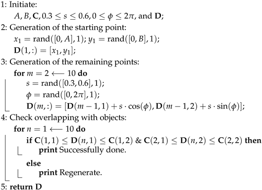
The statistical models proposed in [55] for PL and RMS delay spread for realistic ICU ward and FTPR settings. Specifically, Twenty random trajectories were analyzed, each consisting of 10 consecutive points per scenario. Successive steps in a trajectory were created using randomly chosen starting points, directions, and step lengths. Furthermore, the mobile user advances toward the next sample point at each position along the trajectory [53]. The width A and length B of the considered scenario and the matrix C2×2, which stores the boundaries of the valid area in a hospital room, are initialized. It is crucial to note that the step direction angle is chosen uniformly. The matrix D10×2 stores the coordinates of each sample point randomly generated along the trajectory. The algorithm then verifies whether the points on the trajectory lie within the eligible region. Then, the CIR at each sample point is determined for every photodetector on the mobile user. The extracted CIRs are used to compute the PL and RMS delay spread. The author [55] then visualized the obtained PL and RMS delay spread through histograms accompanied by best-fit curves for D1–D3 in both the ICU ward and FTPR. The random trajectory generator algorithm is described in Algorithm 1.
Extensive simulation studies as described in [55] demonstrate that the log-normal distribution provides a good fit for both path loss and RMS delay spread histograms as given by
where and denote location and scale parameters, respectively.
| Algorithm 1: Random Trajectory Generator |
 |
2.2. Proposed Q-Learning-based Adaptive Modulation Scheme
Adaptive modulation presents a complex challenge within the context of RL due to the volatile and dynamic characteristics of the VLC-driven MBSN system. We start by providing a brief overview of RL and then delve into the Q-learning-based adaptive modulation scheme.
2.2.1. Reinforcement Learning-Based Adaptive Modulation
Reinforcement learning is an ML approach focused on an agent’s dynamic engagement with its surroundings, aiming to develop optimal decision-making strategies that accumulate maximum rewards over time. Unlike supervised learning’s reliance on comprehensive labeled datasets, RL agents acquire knowledge through continuous trial and error.
Among popular RL algorithms, Q-learning is frequently employed to handle Markov Decision Processes (MDPs). Grasping Q-learning starts with understanding its foundational components. S represents the state space, which includes the perceived states s that the agent observes in the environment. Also, A defines the action space, specifying the set of possible actions a that the agent is able to perform in every state. Then, the immediate reward function, , determines the reward acquired right once the agent performs a specific action in a given state. Furthermore, represents the policy, which defines the mapping between observed states and the corresponding actions for the agent. According to the selected policy, the Q-function estimates the cumulative future reward, discounted over time, that results from taking a particular action in a given state. The algorithm then updates the Q-values through the following process.
where represent the learning rate, denotes discount factor, denotes the next state, and represent the possible actions. At its core, Q-learning strives to to derive an optimal policy such that over time, the expected cumulative reward is maximized. This optimal policy is using the following expression
One widely used method for balancing exploration and exploitation is the -greedy strategy.
2.2.2. Q-Learning-Based Adaptive Modulation
For the adaptive modulation optimization problem, the tuple (, ) is defined as the state space, where the action space comprises the available modulation orders, and denotes the quantized received signal-to-noise ratio. Consequently, when the agent modifies the modulation order for a specific channel state, it encounters a new state within the state space. By formulating the problem as an MDP, it becomes suitable for solution using the Q-learning algorithm. Figure 6 demonstrates how patient mobility and agent actions jointly drive state transitions.
Our model does not account for state changes resulting from human movements. Instead, the MDP for Q-learning-based adaptive modulation involves state transitions driven solely by the decisions made by the agent under the current CIR. It is important to emphasize that the speed of the patient is slow enough to allow the agent to explore each state thoroughly. Moreover, after training is completed, the modulation order is chosen by the agent based on initial channel observations. The received SNR is given by
Here, P denotes the transmitted optical power, represents the noise power, and refers to the channel DC-gain, which can be expressed as
where M and are as defined in Eqn. 1.
represents the reward function, which measures the throughput resulting from taking action a in state s within the given environment and is given as follows
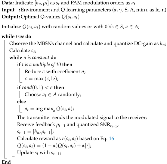
Here, represents the required target symbol error rate. Furthermore, the -greedy approach is used, with a high initial value to facilitate exploration in the early learning stages. During the early stages of learning, the agent selects random actions, gaining valuable insights into the environment. Over time, is decreased to favor exploitation over exploration, encouraging the agent to follow the learned policy. Algorithm 2 outlines the introduced Q-learning-based adaptive modulation scheme.
| Algorithm 2: Q-learning-based Adaptive Modulation for VLC-based MBSN |
 |
2.3. Proposed LSTM-Based Channel Parameter Estimation
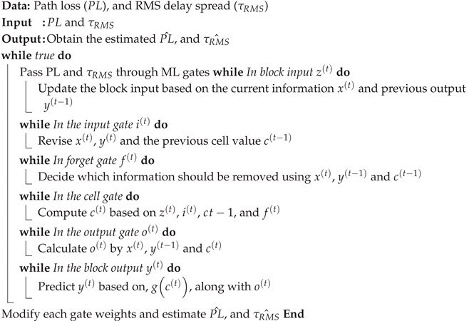
Long Short-Term Memory (LSTM) is a special RNN type consisting of an input gate , forget gate , cell gate , and output gate [56]. This algorithm allows for the prediction of random walks by the user mobile over random trajectories without knowing the sample points, and it also resolves the vanishing gradient problem. The general structure is illustrated in Figure 7. Furthermore, LSTM is capable of handling complex and dynamic propagation environments with higher prediction accuracy, adaptability, and performance, unlike traditional methods [57]. LSTM networks excel in handling sequential data, where the order of data points is both significant and highly correlated. They are designed to iteratively learn these correlations, enabling them to estimate future data points based on past observations. This capability, combined with their memory cell and gating mechanism, allows LSTMs to effectively capture long-range temporal dependencies and adapt to the continuous fluctuations of wireless communication channels. Even in scenarios with high variability over time, their ability to selectively remember or forget information makes them an ideal choice for modeling dynamic channel conditions and user mobility in VLC-based MBSNs. LSTM starts by updating the block input using the current information together with the last LSTM output in the form of
where , , and are the weights with the input, output, and the bias weight vector, respectively. The estimated information could be found by the current cell value and the output gate as follows
where ⊙ is the point-wise multiplication of two vectors along with . The algorithmic details are outlined in Algorithm 3, which calculates the gradients necessary for adjusting the weights within each gate.
| Algorithm 3: ML LSTM-based Path Loss and RMS Delay Spread Estimation for VLC-based MBSNs |
 |
In evaluating the performance of the ML-based system, we utilized Root Mean Squared Error (RMSE) as the loss function. RMSE is widely favored in VLC-based MBSNs for its ability to directly quantify the accuracy of channel parameter estimations, such as path loss and RMS delay spread. By highlighting errors in the estimated values, RMSE provides crucial insights into how well the system models real-world conditions. The RMSE function is mathematically defined as follows
where , , and n represent the actual data, estimated data, and number of data points respectively.
Furthermore, the path loss and RMS delay spread were used as input features for training the LSTM. The dataset was split into an 80% training set and a 20% validation set. Data preprocessing, including normalization, was applied to improve training stability and enhance the model’s performance. Moreover, the LSTM architecture consists of 55 neurons in the hidden layer, designed to balance model complexity and the capacity to represent patterns in the sequential data. A dropout layer with a rate of 0.4 was introduced to mitigate overfitting, followed by a fully connected layer and a regression layer to estimate real value output. The model was trained using the Adam optimization algorithm, which effectively controls training speed, convergence, and generalization performance. The training was conducted over 400 epochs to ensure robust learning. These parameters were selected based on the practical implementation of ML in VLC systems, ensuring their relevance and applicability to real-world scenarios, such as [58]. Other design characteristics of the LSTM are presented in Table 5
To determine the time complexity of the designed LSTM model, let B represent the effective batch size during training, H the number of hidden units, and F the number of input features. The total number of operations performed per iteration is approximately given by .
3. Simulation Results
A site-specific non-sequential ray tracing technique [51] is employed within the ICU ward and FTPR hospital scenarios to find the CIRs. Both scenarios utilized CAD objects to obtain the dependent wavelength reflectances and the specific luminaries on the ceilings and PDs arranged within the human body. The luminaries selected are distributed to ensure the minimum uniformity illuminance ratio and minimum average illumination level. Moreover, three node sensors are attached to the mobile human where (D1) is positioned on the shoulder, (D2) on the wrist, and (D3) on the ankle to form the MBSNs [51]. The first room is an ICU ward with four patients in their beds, a healthcare provider who walks randomly within the room, a chair, and a desk. Furthermore, the second scenario is an FTPR with a patient in the bed, a healthcare provider who is also considered walking randomly in the room, furniture, a sofa, and a restroom. The ICU ward has 11.5 m × 6.5 m × 3 m room dimensions with 15 luminaries on the ceiling, whereas the FTPR has 7 m × 5 m × 3 m dimensions with 8 luminaries. Furthermore, 20 random trajectories with 10 successive points in each scenario are considered while the step length and direction are uniformly selected. After generating the random trajectory movements, path loss and RMS delay spread are obtained from the CIR, which considers real-life specifications and serves as inputs for different ML algorithms to estimate PL and RMS delay spread.
3.1. Q-Learning-Based Adaptive Modulation
In this study, the CIRs obtained from a previous work [53] were used. The evaluation focused on SE performance across multiple schemes: the Q-learning-based adaptive modulation, the KNN-based adaptive modulation, a non-adaptive scheme, and the optimal achievable SE. Additionally, for all channels, a flat fading channel model is used, given its relevance for the low data rates characteristic of MBSN applications, which has demonstrated satisfactory results for the study. The parameters for the adaptive modulation algorithm and a summary of the system model are presented in Table 6.
The Q-learning-based modulation scheme does not require CSI for its model training; instead, it acquires knowledge by extensively exploring its environment. Even as the exploration factor gradually diminishes, exploration continues, allowing dynamic adjustment to changes in both the system model and its environment. The algorithm fundamentally relies on these two properties. As depicted in Figure 8, during the initial stages of training, the Q-learning-based adaptive modulation starts with an exploration phase, which results in an initial that is higher than the intended target. Over time, the steadily declines. After accumulating sufficient information in the Q table, the agent shifts to making more deterministic choices through the use of a greedy strategy. Furthermore, When the system adopts greedy decision-making the does not experience a significant drop; instead, it fluctuates just below the . Since excessively low values are not considered ideal, this outcome aligns with the goal of optimizing SE.
The SE performance of various methods is depicted in Figure 9. Optimal SE—defined as the maximum SE that still fulfills the necessary —is the benchmark for performance. In this scenario, the KNN approach is configured to utilize 60% of the CIRs, corresponding to 12 trajectories, with K set to 3 for nearest neighbor calculation. Unlike the non-adaptive method that resorts to binary PAM to achieve the target , both the KNN and Q-learning strategies bring about considerable improvements in SE. As illustrated in Figure 9 (a), Figure 9 (b), and Figure 9 (e), there are instances where the KNN method’s SE surpasses the optimal level, suggesting that the desired is not achieved in those occurrences.
Unlike other methods, the Q-learning approach consistently satisfies the desired in all figures. Nonetheless, the SE may fall short of the optimal value in some instances as a result of quantization level limitations, particularly when the optimal is near . In these cases, the method favors meeting the target, taking a more conservative approach. Although raising the quantization levels improves precision, it comes at the cost of greater complexity. Additionally, the continuous exploration process contributes to this behavior.
In addition, Significant SE improvements are observed when employing a Q-learning-based adaptive modulation scheme over a non-adaptive approach. In the ICU ward, the observed increases are 151%, 178%, and 81% for D1, D2, and D3, respectively. Additionally, our model exhibits substantial SE gains within the FTPR scenario, specifically achieving 304%, 303%, and 151% for D1, D2, and D3, respectively. This higher SE improvement in the FTPR scenario, in contrast to the ICU ward, indicates that the channel DC gain range in FTPR is significantly broader, consistent with the results reported in [53].
Moreover, PDs placed on the Shoulder (D1) and Wrist (D2) show greater SE improvements with the learning-based adaptive modulation approach, in contrast to those placed on the Ankle (D3), across both scenarios. The disparity results from the sinusoidal pattern of the DC gain in D1 and D2, produced by their line-of-sight (LOS) rays. Unlike D1 and D2, D3 is mostly influenced by NLOS rays, producing a smoother DC gain pattern. Due to the narrow range of DC gain, D3 exhibits decreased SE compared to other nodes.
3.2. LSTM-Based Path Loss and RMS Delay Spread Estimation
After comprehensive simulation results using various ML techniques, the estimated path loss and RMS delay spread for D1–D3 in both ICU ward and FTPR scenarios were obtained. The observed RMSE values for these scenarios are detailed in Table 7 and Table 8. The LSTM algorithm consistently outperforms other models in both hospital settings, achieving the lowest RMSE for path loss and RMS delay spread, as illustrated in Figure 10 and Figure 11. This demonstrates LSTM’s superior performance in minimizing prediction errors.
Based on Table 7, it is observed that the estimated path loss for D1 within the ICU ward scenario has the highest RMSE compared to D2 and D3, confirming the results in [55], where the log-normal distribution of D1 has the highest variance value of 0.0262 compared to D2 and D3 with variances of 0.0176 and 0.0169, respectively, since higher variance results in higher estimated RMSE. Furthermore, based on Table 8, it is observed that D3 has the highest RMSE compared to D1 and D2 within the FTPR scenario, which also confirms the results in [55], where the log-normal distribution of D3 has the highest variance value of 0.0168 compared to D1 and D2 with variances of 0.0123 and 0.0119, respectively, since the highest detector variance shows higher estimated RMSE.
It is also observed from Table 7 that the estimated RMS delay spread for D1 within the ICU ward scenario has the highest RMSE compared to D2 and D3, which is expected as the log-normal distribution of D1 obtained in [55] has the highest variance of 0.0975, while D2 and D3 have variances of 0.0847 and 0.0780, respectively, indicating that the higher variance of D1 contributes to its increased estimated RMSE. However, based on Table 8, it is observed that D3 has the highest RMSE compared to D1 and D2, confirming the results in [55], where the log-normal distribution of D3 has the highest variance value of 0.0967 compared to D1 and D2 with variances of 0.0659 and 0.0747, respectively, further illustrating that the higher variance leads to a higher estimated RMSE.
A practical complexity analysis is presented to verify the selection of LSTM, evaluating both training and prediction times within the ICU ward and FTPR settings, as shown in Table 9 and Table 10, respectively. The focus is directed toward LSTM, GRU, and RNN, given their advantages and extensive use in MBSN applications. These models as we stated before are designed for sequential data regression tasks, excelling at capturing temporal dependencies, making them well-suited for time-series prediction and real-time health monitoring.
Based on Table 9, it is found that within the ICU ward, LSTM outperforms GRU and RNN in terms of execution time for D1-D3 across both PL and RMS delay spread, thereby verifying the choice of LSTM. The execution times for D1-D3 PL within the ICU ward were 68.051 s, 65.854 s, and 66.229 s, respectively, while the RMS delay spread execution times for the ICU ward were 69.946 s, 68.786 s, and 68.948 s, respectively. Similarly, based on Table 10, the analysis results indicate that LSTM is also preferable within the FTPR for D1–D3 in terms of execution time for both PL and RMS delay spread. The execution times for D1-D3 PL within the FTPR were 69.112 s, 70.484 s, and 69.919 s, respectively, whereas for the RMS delay spread within the FTPR, they were 69.740 s, 70.220 s, and 69.650 s, respectively.
These results align with expectations, as LSTM’s architecture, with its long memory, cell states, and ability to capture long-term sequential correlations, is particularly well-suited for VLC-based MBSN path loss and RMS delay data. Even though the RMSE was relatively comparable to other methods like GRU, our design achieved low complexity, moderate parameter tuning, and faster training times compared to other models while ensuring the same standard practices. LSTM’s performance demonstrates a superior alignment with the intricate temporal dependencies in our data, solidifying its position as the most effective and reliable model for this purpose.
When implemented in real hospital settings, LSTM models face practical challenges, including energy consumption, system integration, computational complexity, and the dynamic nature of healthcare environments. To address such challenges, authors in [59] applied LSTM to optimize Hospital Management Systems performance, analyzing historical and real-time data across two resource allocation scenarios. The model demonstrated a strong alignment between predicted and actual outcomes, with residual errors tightly around zero. Whereas in [60], the authors used LSTM to predict patient visits at a community health center based on 43 months of historical data. The results showed that LSTM outperformed the other models, achieving a Mean Absolute Percentage Error (MAPE) of 4.714, Mean Absolute Error (MAE) of 154.796, and an RMSE of 167.631. This indicates that the LSTM model can maintain high operational accuracy and robustness while adapting to dynamic scenarios. Furthermore, the results suggest that challenges such as computational complexity can be mitigated by the model’s ability to learn temporal patterns efficiently. These findings highlight the potential of LSTM models to overcome key challenges in real hospital environments, including reducing patient wait times, improving staff scheduling, and enhancing overall patient outcomes.
Therefore, throughout this paper, we established ML algorithms to estimate channel characteristic parameters, namely PL and RMS delay spread, in indoor VLC-based MBSNs within two hospital environments. This work contributes to the overall understanding of the IoMT and its integration into 6G networks. These findings underline the significance of ML-driven channel modeling for advancing MBSN technologies in hospital environments, paving the way for more efficient and reliable communication systems in 6G-enabled healthcare.
4. Conclusions
This paper introduces realistic statistical models for channel modeling in hospital environments and ML-based algorithms for adaptive modulation and channel parameter estimation in VLC-based MBSNs, considering wavelength dependency, random trajectories, and real-world hospital scenarios.
In our efforts to improve SE performance, we explored multiple modulation schemes: a Q-learning-based adaptive modulation, a KNN-based adaptive modulation, and a non-adaptive scheme that mainly serve as a reference point. The Q-learning-based modulation scheme demonstrated dynamic adaptability to changes in both the system model and the environment, all without the need for explicit CSI. Meanwhile, by balancing exploration and exploitation, the Q-learning algorithm gradually improved its SER performance until the required SER was reached. Compared to the non-adaptive approach, the KNN method demonstrated enhanced SE, though it occasionally did not satisfy the required SER. Conversely, although the Q-learning method reliably met the target SER, its SE occasionally lagged behind the optimal value due to quantization restrictions and a cautious strategy close to the desired SER. Enhancing precision is possible by increasing quantization levels, though this comes at the cost of added complexity. Future work should focus on refining the quantization process or adopting neural networks as a replacement. Moreover, other adaptive modulation algorithms can be explored to improve SE performance in VLC-based MBSNs. In addition, in environments with high data rates—where delay plays a key role in transmission—advanced RL models can be leveraged to monitor user mobility.
Beyond modulation, the study also explored channel parameter estimation for reliable VLC communication. The method used in this section was LSTM, which proved to be the best-performing ML technique. Simulation results show that in the ICU ward, D1 has the highest RMSE for path loss (1.6797 dB) and RMS delay spread (1.0567 ns). In the FTPR scenario, D3 shows the highest RMSE for path loss (1.0652 dB) and RMS delay spread (0.7657 ns). Accurate estimation of VLC channel parameters, such as DC gain and RMS delay spread, is vital for robust communication systems, with ML algorithms improving reliability and efficiency. These findings show that the performance of ML algorithms for estimating path loss and RMS delay spread in VLC-based MBSNs depends heavily on the photo-detector location and scenario geometry, which are key in VLC channel modeling.
Author Contributions
Conceptualization, F. Miramirkhani; methodology, F. Miramirkhani, Bilal Antaki and Ahmed Dalloul; software,Bilal Antaki and Ahmed Dalloul; validation, F. Miramirkhani, Bilal Antaki and Ahmed Dalloul; formal analysis, Bilal Antaki and Ahmed Dalloul; writing—original draft preparation, F. Miramirkhani, Bilal Antaki and Ahmed Dalloul; writing—review and editing, F. Miramirkhani, Bilal Antaki and Ahmed Dalloul; supervision,F. Miramirkhani; project administration, F. Miramirkhani. All authors have read and agreed to the published version of the manuscript.
Conflicts of Interest
The authors declare no conflicts of interest.
References
- Letaief, K.B.; Chen, W.; Shi, Y.; Zhang, J.; Zhang, Y.J.A. The Roadmap to 6G: AI Empowered Wireless Networks. IEEE Communications Magazine 2019, 57, 84–90. [Google Scholar] [CrossRef]
- Yang, P.; Xiao, Y.; Xiao, M.; Li, S. 6G Wireless Communications: Vision and Potential Techniques. IEEE Network 2019, 33, 70–75. [Google Scholar] [CrossRef]
- Mitra, P.; Bhattacharjee, R.; Chatterjee, T.; De, S.; Karmakar, R.; Ghosh, A.; Adhikari, T. Towards 6G Communications: Architecture, Challenges, and Future Directions. In Proceedings of the 2021 12th International Conference on Computing Communication and Networking Technologies (ICCCNT); 2021; pp. 1–7. [Google Scholar] [CrossRef]
- Kaur, J.; Khan, M.A.; Iftikhar, M.; Imran, M.; Emad Ul Haq, Q. Machine Learning Techniques for 5G and Beyond. IEEE Access 2021, 9, 23472–23488. [Google Scholar] [CrossRef]
- Kaur, J.; Khan, M.A. Sixth Generation (6G) Wireless Technology: An Overview, Vision, Challenges and Use Cases. In Proceedings of the 2022 IEEE Region 10 Symposium (TENSYMP); 2022; pp. 1–6. [Google Scholar] [CrossRef]
- Wang, C.X.; You, X.; Gao, X.; Zhu, X.; Li, Z.; Zhang, C.; Wang, H.; Huang, Y.; Chen, Y.; Haas, H.; et al. On the road to 6G: Visions, requirements, key technologies, and testbeds. IEEE Communications Surveys & Tutorials 2023, 25, 905–974. [Google Scholar]
- Ariyanti, S.; Suryanegara, M. Visible Light Communication (VLC) for 6G Technology: The Potency and Research Challenges. In Proceedings of the 2020 Fourth World Conference on Smart Trends in Systems, Security and Sustainability (WorldS4); 2020; pp. 490–493. [Google Scholar] [CrossRef]
- Abdel Hakeem, S.A.; Hussein, H.H.; Kim, H. Vision and research directions of 6G technologies and applications. Journal of King Saud University - Computer and Information Sciences 2022, 34, 2419–2442. [Google Scholar] [CrossRef]
- Niarchou, E.; Boucouvalas, A.C.; Ghassemlooy, Z.; Alves, L.N.; Zvanovec, S. Visible Light Communications for 6G Wireless Networks. In Proceedings of the 2021 Third South American Colloquium on Visible Light Communications (SACVLC); 2021; pp. 01–06. [Google Scholar] [CrossRef]
- Saxena, V.N.; Dwivedi, V.K.; Gupta, J. Machine learning in visible light communication system: A survey. Wireless Communications and Mobile Computing 2023, 2023, 3950657. [Google Scholar] [CrossRef]
- Zwaag, K.M.V.D.; Marinho, M.P.; Costa, W.D.S.; De Assis Souza Dos Santos, F.; Bastos-Filho, T.F.; Rocha, H.R.O.; Segatto, M.E.V.; Silva, J.A.L. A Manchester-OOK Visible Light Communication System for Patient Monitoring in Intensive Care Units. IEEE Access 2021, 9, 104217–104226. [Google Scholar] [CrossRef]
- Kurunathan, H.; Indhumathi, R.; Gaitán, M.G.; Taramasco, C.; Tovar, E. VLC-enabled monitoring in a healthcare setting: Overview and Challenges. In Proceedings of the 2023 South American Conference On Visible Light Communications (SACVLC); 2023; pp. 135–140. [Google Scholar] [CrossRef]
- Zakerabasali, S.; Ayyoubzadeh, S.M. Internet of Things and healthcare system: A systematic review of ethical issues. Health Science Reports 2022, 5, e863. [Google Scholar] [CrossRef]
- Zhu, X.; Wang, C.X.; Huang, J.; Chen, M.; Haas, H. A Novel 3D Non-Stationary Channel Model for 6G Indoor Visible Light Communication Systems. IEEE Transactions on Wireless Communications 2022, 21, 8292–8307. [Google Scholar] [CrossRef]
- Fernández, B.; Játiva, P.P.; Azurdia-Meza, C.A.; Boettcher, N.; Zabala-Blanco, D.; Gaitán, M.G.; Soto, I. Performance Analysis of a VLC System Applied to a Hospital Environment for IoT-Based Smart Patient Monitoring. In Proceedings of the 2024 14th International Symposium on Communication Systems, Networks and Digital Signal Processing (CSNDSP); 2024; pp. 615–620. [Google Scholar] [CrossRef]
- Pathak, P.H.; Feng, X.; Hu, P.; Mohapatra, P. Visible light communication, networking, and sensing: A survey, potential and challenges. IEEE communications surveys & tutorials 2015, 17, 2047–2077. [Google Scholar]
- Arnon, S. Advanced optical wireless communication systems; Cambridge university press, 2012.
- Ghassemlooy, Z.; Popoola, W.; Rajbhandari, S. Optical wireless communications: system and channel modelling with Matlab®; CRC press, 2019.
- Rahman, M.; Sarwar, H.; Kader, M.A.; Gonçalves, T.; Tin, T.T. Review and Empirical Analysis of Machine Learning-Based Software Effort Estimation. IEEE Access 2024, 12, 85661–85680. [Google Scholar] [CrossRef]
- Zhang, S. Challenges in KNN Classification. IEEE Transactions on Knowledge and Data Engineering 2022, 34, 4663–4675. [Google Scholar] [CrossRef]
- Zhou, C.; Yu, W.; Huang, K.; Zhu, H.; Li, Y.; Yang, C.; Sun, B. A New Model Transfer Strategy Among Spectrometers Based on SVR Parameter Calibrating. IEEE Transactions on Instrumentation and Measurement 2021, 70, 1–13. [Google Scholar] [CrossRef]
- Yu, H.; Lu, J.; Zhang, G. An Online Robust Support Vector Regression for Data Streams. IEEE Transactions on Knowledge and Data Engineering 2022, 34, 150–163. [Google Scholar] [CrossRef]
- Gizzini, A.K.; Chafii, M. RNN Based Channel Estimation in Doubly Selective Environments. IEEE Transactions on Machine Learning in Communications and Networking 2024, 2, 1–18. [Google Scholar] [CrossRef]
- Mao, S.; Sejdić, E. A Review of Recurrent Neural Network-Based Methods in Computational Physiology. IEEE Transactions on Neural Networks and Learning Systems 2023, 34, 6983–7003. [Google Scholar] [CrossRef]
- Zengeya, T.; Vincent Fonou-Dombeu, J. A Review of State of the Art Deep Learning Models for Ontology Construction. IEEE Access 2024, 12, 82354–82383. [Google Scholar] [CrossRef]
- Brandão Lent, D.M.; Novaes, M.P.; Carvalho, L.F.; Lloret, J.; Rodrigues, J.J.P.C.; Proença, M.L. A Gated Recurrent Unit Deep Learning Model to Detect and Mitigate Distributed Denial of Service and Portscan Attacks. IEEE Access 2022, 10, 73229–73242. [Google Scholar] [CrossRef]
- Daniels, R.C.; Caramanis, C.M.; Heath, R.W. Adaptation in convolutionally coded MIMO-OFDM wireless systems through supervised learning and SNR ordering. IEEE Transactions on vehicular Technology 2009, 59, 114–126. [Google Scholar] [CrossRef]
- Mashhadi, S.; Ghiasi, N.; Farahmand, S.; Razavizadeh, S.M. Deep reinforcement learning based adaptive modulation with outdated CSI. IEEE Communications Letters 2021, 25, 3291–3295. [Google Scholar] [CrossRef]
- Leite, J.P.; de Carvalho, P.H.P.; Vieira, R.D. A flexible framework based on reinforcement learning for adaptive modulation and coding in OFDM wireless systems. In Proceedings of the 2012 IEEE Wireless Communications and Networking Conference (WCNC). IEEE; 2012; pp. 809–814. [Google Scholar]
- Lee, D.; Sun, Y.G.; Kim, S.H.; Sim, I.; Hwang, Y.M.; Shin, Y.; Kim, D.I.; Kim, J.Y. DQN-based adaptive modulation scheme over wireless communication channels. IEEE Communications Letters 2020, 24, 1289–1293. [Google Scholar] [CrossRef]
- Elwekeil, M.; Jiang, S.; Wang, T.; Zhang, S. Deep convolutional neural networks for link adaptations in MIMO-OFDM wireless systems. IEEE Wireless Communications Letters 2018, 8, 665–668. [Google Scholar] [CrossRef]
- Fu, Q.; Song, A. Adaptive modulation for underwater acoustic communications based on reinforcement learning. In Proceedings of the OCEANS 2018 MTS/IEEE Charleston. IEEE; 2018; pp. 1–8. [Google Scholar]
- Su, W.; Lin, J.; Chen, K.; Xiao, L.; En, C. Reinforcement learning-based adaptive modulation and coding for efficient underwater communications. IEEE access 2019, 7, 67539–67550. [Google Scholar] [CrossRef]
- Byun, J.; Cho, Y.H.; Im, T.; Ko, H.L.; Shin, K.; Kim, J.; Jo, O. Iterative learning for reliable link adaptation in the Internet of Underwater Things. IEEE Access 2021, 9, 30408–30416. [Google Scholar] [CrossRef]
- Zhang, Y.; Zhu, J.; Wang, H.; Shen, X.; Wang, B.; Dong, Y. Deep reinforcement learning-based adaptive modulation for underwater acoustic communication with outdated channel state information. Remote Sensing 2022, 14, 3947. [Google Scholar] [CrossRef]
- Rizi, R.B.; Forouzan, A.R.; Miramirkhani, F.; Sabahi, M.F. Machine Learning-Driven Adaptive Modulation for VLC-Enabled Medical Body Sensor Networks. Iranian Journal of Electrical & Electronic Engineering 2024, 20. [Google Scholar]
- Cahyadi, W.A.; Jeong, T.I.; Kim, Y.H.; Chung, Y.H.; Adiono, T. Patient monitoring using visible light uplink data transmission. In Proceedings of the 2015 International Symposium on Intelligent Signal Processing and Communication Systems (ISPACS). IEEE; 2015; pp. 431–434. [Google Scholar]
- Lebas, C.; Sahuguede, S.; Julien-Vergonjanne, A.; Combeau, P.; Aveneau, L. Infrared and visible links for medical body sensor networks. In Proceedings of the 2018 Global LIFI Congress (GLC). IEEE; 2018; pp. 1–6. [Google Scholar]
- Candia, D.A.; Játiva, P.P.; Azurdia Meza, C.; Sánchez, I.; Ijaz, M. Performance analysis of the particle swarm optimization algorithm in a vlc system for localization in hospital environments. Applied Sciences 2024, 14, 2514. [Google Scholar] [CrossRef]
- Guaña-Moya, J.; Román Cañizares, M.; Palacios Játiva, P.; Sánchez, I.; Ruminot, D.; Lobos, F.V. Comprehensive survey on VLC in e-healthcare: Channel coding schemes and modulation techniques. Applied Sciences 2024, 14, 8912. [Google Scholar] [CrossRef]
- Játiva, P.P.; Becerra, R.; Azurdia-Meza, C.A.; Zabala-Blanco, D.; Soto, I.; Cañizares, M.R. Extreme Learning Machine Based Channel Estimator and Equalizer for Underground Mining VLC Systems. In Proceedings of the 2021 IEEE Latin-American Conference on Communications (LATINCOM); 2021; pp. 1–6. [Google Scholar] [CrossRef]
- Alkandari, Y.; Ijaz, M.; Ekpo, S.; Adebisi, B.; Soto, I.; Zamorano-Illanes, R.; Azurdia, C. Optimization of Visible Light Positioning in Industrial Applications using Machine Learning. In Proceedings of the 2023 South American Conference On Visible Light Communications (SACVLC); 2023; pp. 141–146. [Google Scholar] [CrossRef]
- Du, P.; Zhang, S.; Alphones, A.; Chen, C. Faster Deployment for Indoor Visible Light Positioning Using Xgboost Algorithms in Industrial Internet-of-Things. In Proceedings of the IECON 2021 – 47th Annual Conference of the IEEE Industrial Electronics Society; 2021; pp. 1–7. [Google Scholar] [CrossRef]
- Razaz, M.A.; Algaolahi, A.Q.; Makarem, M.A.; Alwardy, E.H. VLC Channel estimation for indoor environment using LSTM. In Proceedings of the 2024 4th International Conference on Emerging Smart Technologies and Applications (eSmarTA); 2024; pp. 1–4. [Google Scholar] [CrossRef]
- Sharma, A.; Keshari, P.; Bhatia, V. LSTM-based Channel Estimator for Optical IRS-Assisted non-Linear VLC Systems. In Proceedings of the 2023 IEEE International Conference on Advanced Networks and Telecommunications Systems (ANTS); 2023; pp. 114–119. [Google Scholar] [CrossRef]
- Ma, Z.; Jia, P.; Han, D.; Zhang, M.; Ghassemlooy, Z.; Wang, L. Deep-Learning-Based Channel Estimation for Multi-wavelength Visible Light Communication System. In Proceedings of the 2022 4th West Asian Symposium on Optical and Millimeter-wave Wireless Communications (WASOWC); 2022; pp. 01–04. [Google Scholar] [CrossRef]
- Ullah, A.; Choi, W.; Coleri, S. Path Loss Estimation and Jamming Detection in Hybrid RF-VLC Vehicular Networks: A Machine-Learning Framework. IEEE Sensors Journal 2023, 23, 31325–31336. [Google Scholar] [CrossRef]
- Salama, W.M.; Aly, M.H.; Amer, E.S. Deep learning based channel estimation optimization in VLC systems. Optical and Quantum Electronics 2023, 55, 79. [Google Scholar] [CrossRef]
- Mitra, R.; Kaddoum, G. Random Fourier Feature-Based Deep Learning for Wireless Communications. IEEE Transactions on Cognitive Communications and Networking 2022, 8, 468–479. [Google Scholar] [CrossRef]
- Naser, S.; Bariah, L.; Muhaidat, S.; Sofotasios, P.C.; Al-Qutayri, M.; Damiani, E.; Debbah, M. Toward Federated-Learning-Enabled Visible Light Communication in 6G Systems. IEEE Wireless Communications 2022, 29, 48–56. [Google Scholar] [CrossRef]
- Donmez, B.; Mitra, R.; Miramirkhani, F. Channel modeling and characterization for VLC-based medical body sensor networks: trends and challenges. IEEE Access 2021, 9, 153401–153419. [Google Scholar] [CrossRef]
- Gu, Z.; Yang, J.; Wang, P. Research on channel modeling technology of visible light communication system based on the ray tracing method. Journal of Physics: Conference Series 2024, 2807, 012043. [Google Scholar] [CrossRef]
- Donmez, B.; Miramirkhani, F. Channel Modeling and Characterization for VLC-based MBSNs Impaired by 3D User Mobility. In Proceedings of the 2021 13th International Conference on Electrical and Electronics Engineering (ELECO). IEEE; 2021; pp. 485–489. [Google Scholar]
- Islim, M.S.; Videv, S.; Safari, M.; Xie, E.; McKendry, J.J.D.; Gu, E.; Dawson, M.D.; Haas, H. The Impact of Solar Irradiance on Visible Light Communications. Journal of Lightwave Technology 2018, 36, 2376–2386. [Google Scholar] [CrossRef]
- Donmez, B.; Miramirkhani, F. Path Loss and RMS Delay Spread Model for VLC-based Patient Health Monitoring System. In Proceedings of the 2022 4th West Asian Symposium on Optical and Millimeter-wave Wireless Communications (WASOWC); 2022; pp. 1–5. [Google Scholar] [CrossRef]
- Guo, J.; Zhang, Q.; Zhao, Y.; Shi, H.; Jiang, Y.; Sun, J. RNN-Test: Towards Adversarial Testing for Recurrent Neural Network Systems. IEEE Transactions on Software Engineering 2022, 48, 4167–4180. [Google Scholar] [CrossRef]
- Van Houdt, G.; Mosquera, C.; Nápoles, G. A review on the long short-term memory model. Artificial Intelligence Review 2020, 53, 5929–5955. [Google Scholar] [CrossRef]
- Shu, Y.H.; Chang, Y.H.; Lin, Y.Z.; Chow, C.W. Real-Time Indoor Visible Light Positioning (VLP) Using Long Short Term Memory Neural Network (LSTM-NN) with Principal Component Analysis (PCA). Sensors 2024, 24, 5424. [Google Scholar] [CrossRef]
- Saxena, A.K.; Dixit, R.R.; Aman-Ullah, A. An LSTM Neural Network Approach to Resource Allocation in Hospital Management Systems. International Journal of Applied Health Care Analytics 2022, 7, 1–12. [Google Scholar]
- Karsanti, H.T.; Ardiyanto, I.; Nugroho, L.E. Deep Learning-Based Patient Visits Forecasting Using Long Short Term Memory. In Proceedings of the 2019 International Conference of Artificial Intelligence and Information Technology (ICAIIT); 2019; pp. 344–349. [Google Scholar] [CrossRef]
Figure 1.
Healthcare network architecture within 6G.
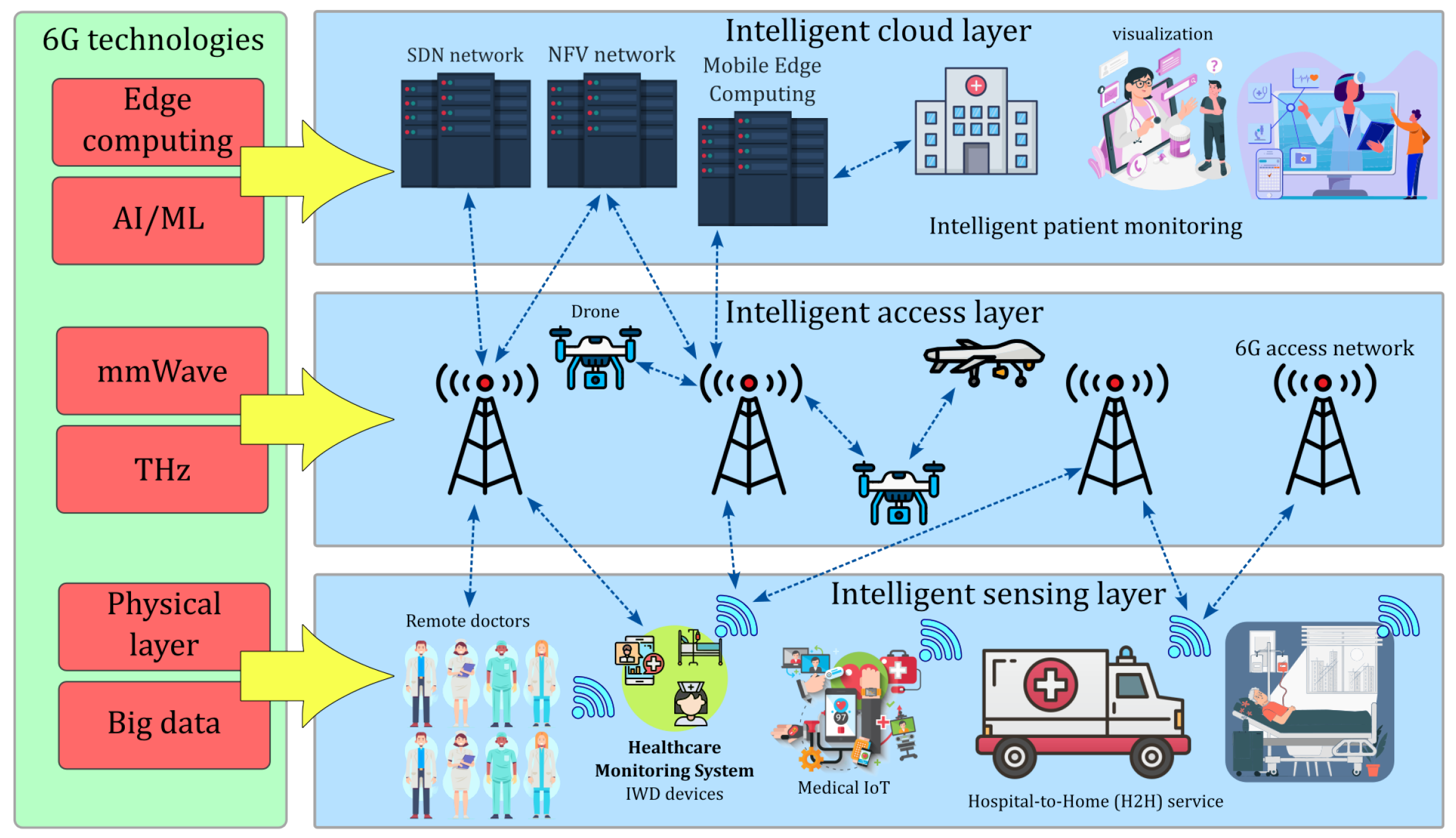
Figure 2.
ML applications in a VLC-Based MBSNs system.
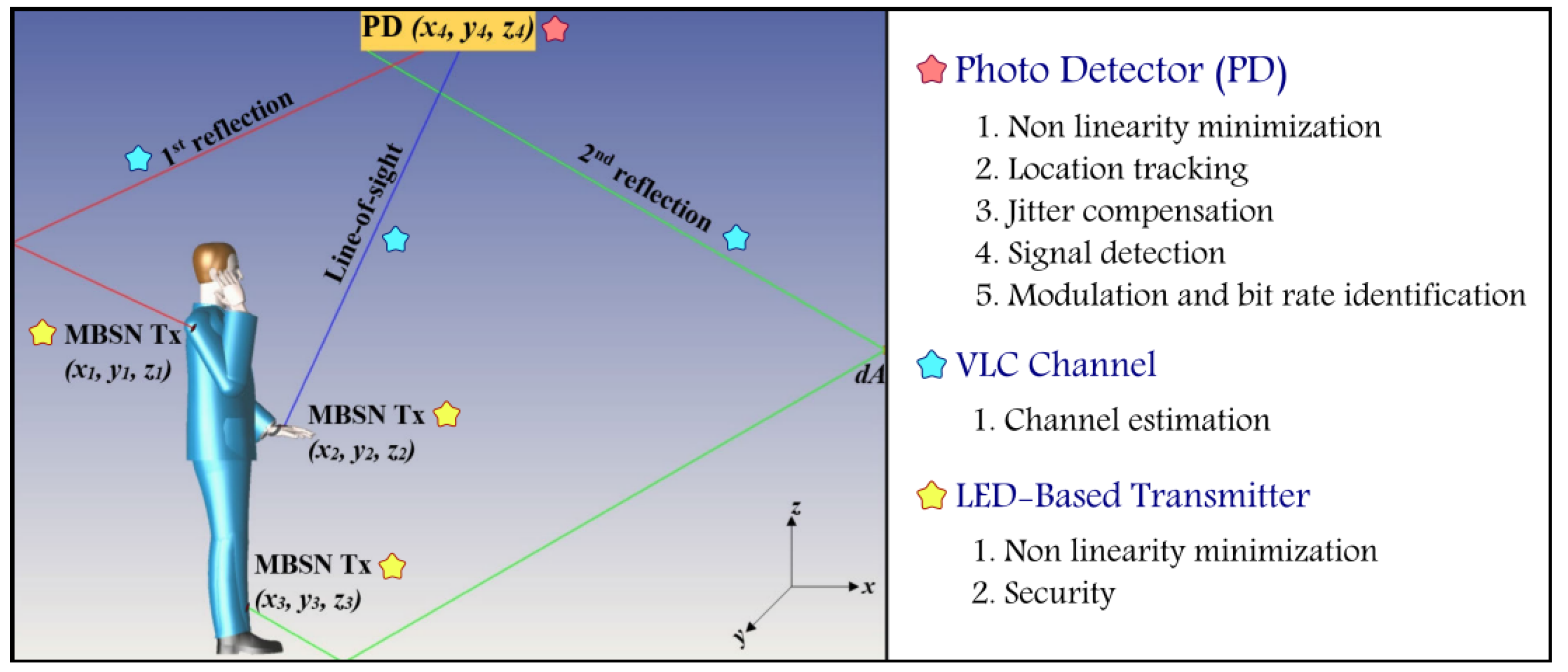
Figure 3.
Site-specific channel modeling steps for VLC-based MBSNs.
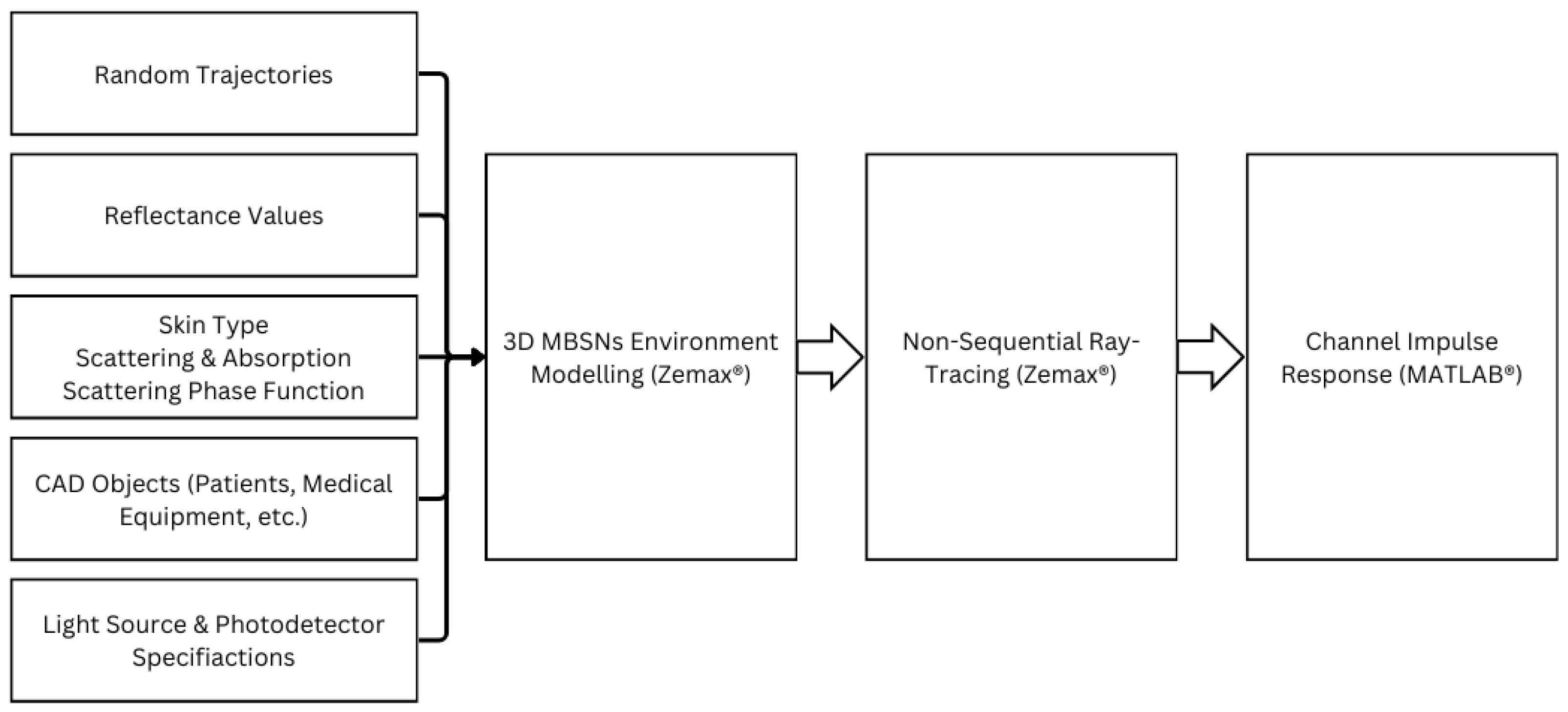
Figure 4.
Hospital settings (a) ICU ward and (b) FTPR. [55].
Figure 4.
Hospital settings (a) ICU ward and (b) FTPR. [55].
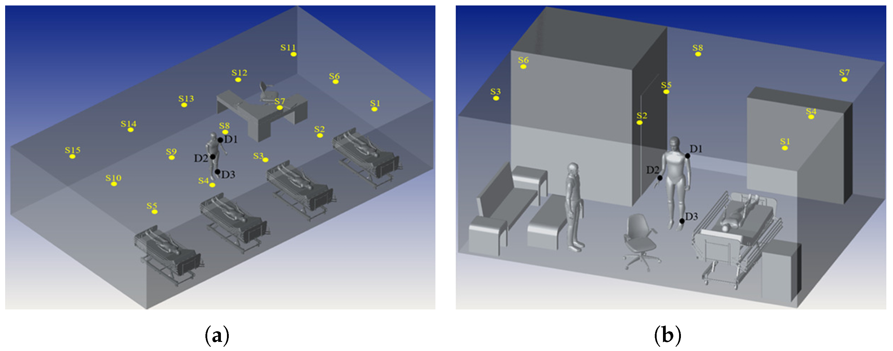
Figure 5.
VLC-based MBSNs system model [36].
Figure 5.
VLC-based MBSNs system model [36].

Figure 6.
Reinforcement learning model applied to adaptive modulation in VLC-based MBSNs [36].
Figure 6.
Reinforcement learning model applied to adaptive modulation in VLC-based MBSNs [36].
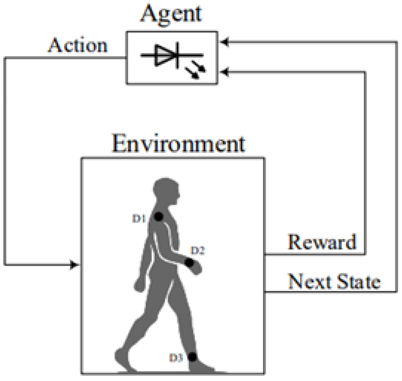
Figure 7.
LSTM architecture to estimate PL and of VLC-based MBSNs.
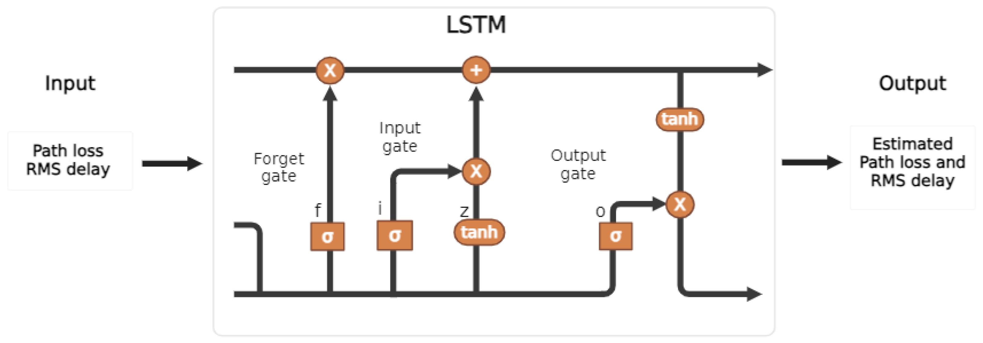
Figure 8.
Training stage of Q-learning based adaptive modulation scheme in ICU ward. (a)-(c) correspond to D1-D3, respectively.
Figure 8.
Training stage of Q-learning based adaptive modulation scheme in ICU ward. (a)-(c) correspond to D1-D3, respectively.
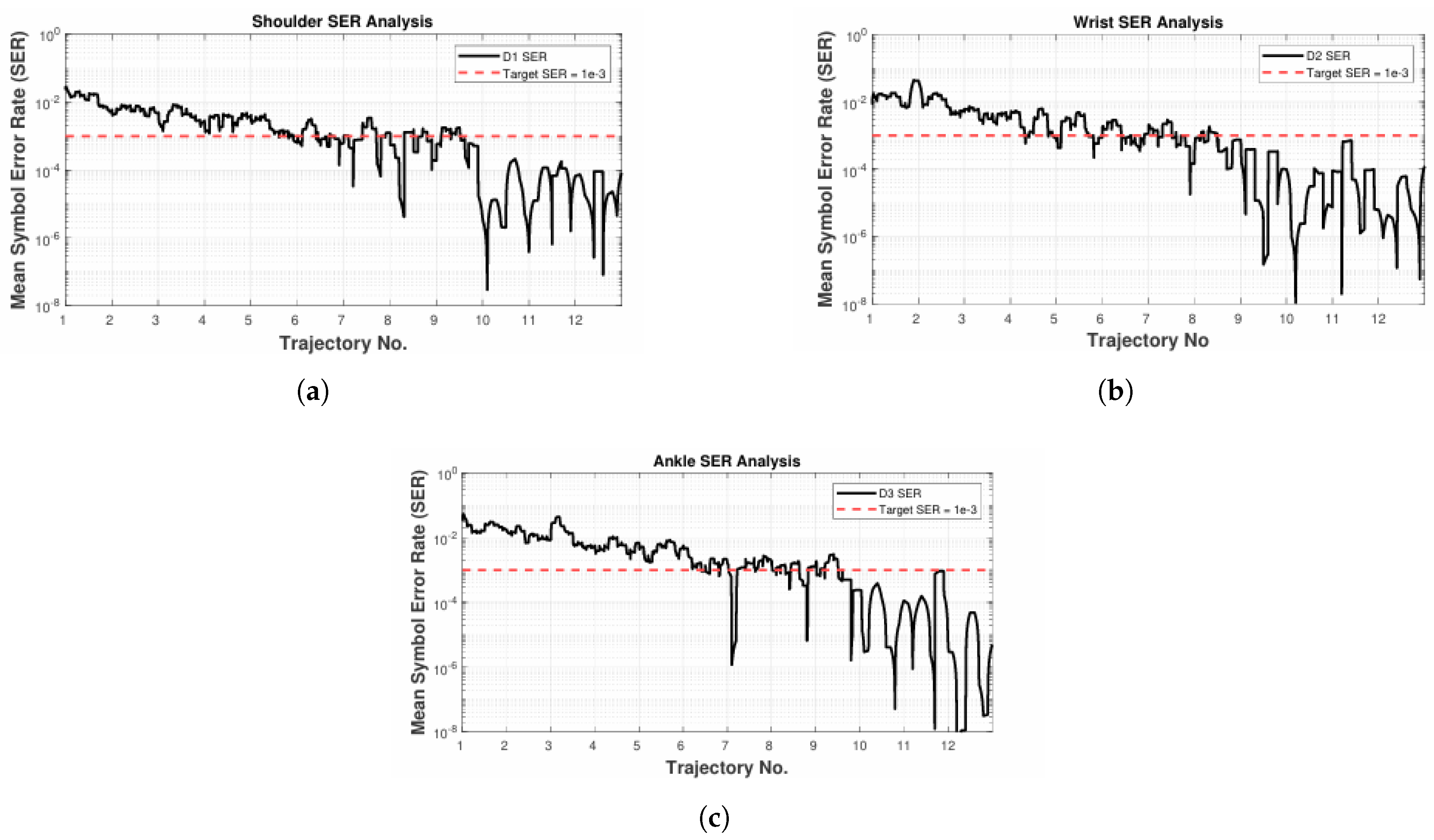
Figure 9.
Spectral efficiency analysis of various modulation schemes in (a,c,e) ICU ward and (b,d,f) FTPR. [36].
Figure 9.
Spectral efficiency analysis of various modulation schemes in (a,c,e) ICU ward and (b,d,f) FTPR. [36].
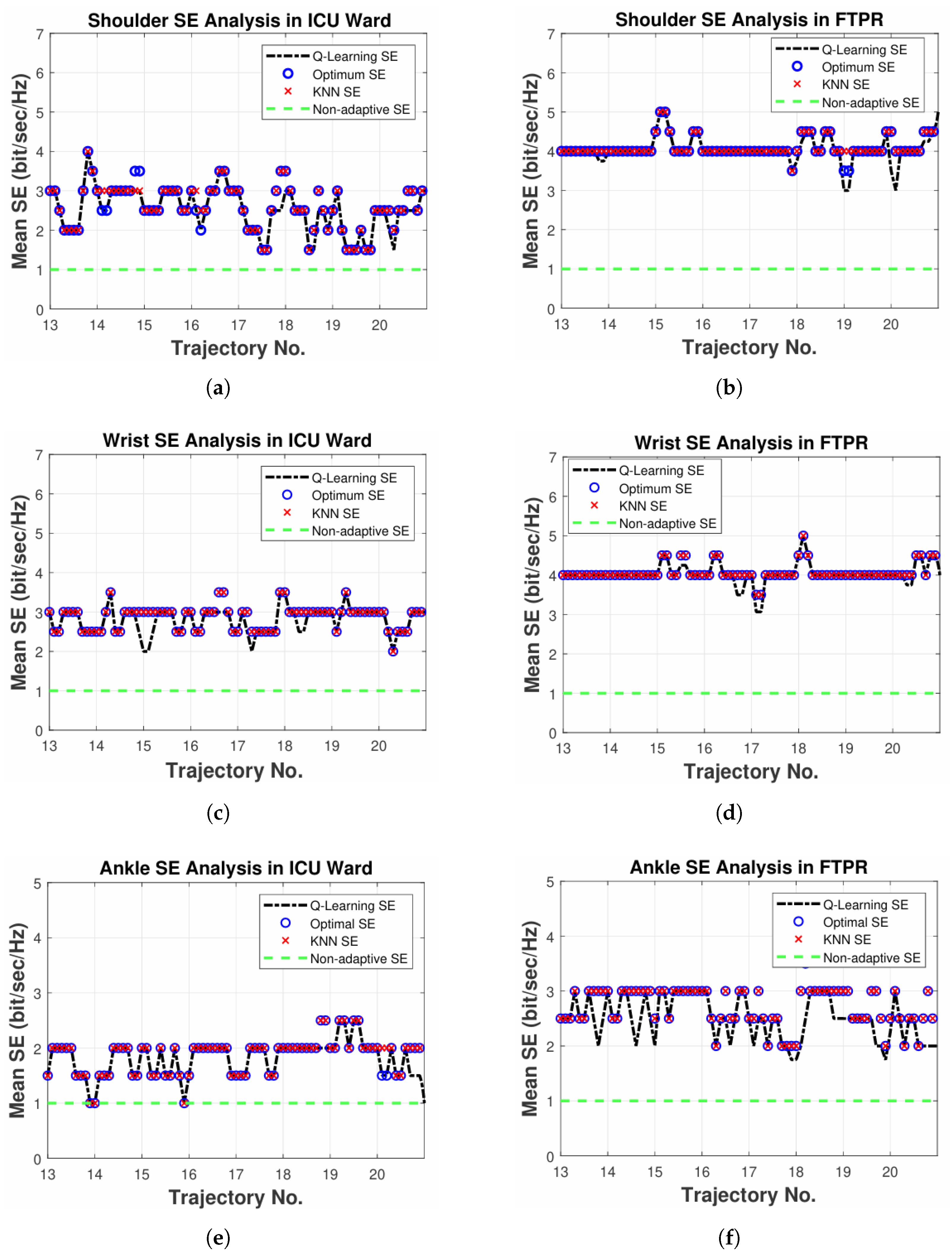
Figure 10.
(a,c,e) estimated path loss and (b,d,f) RMS delay distribution in ICU ward.
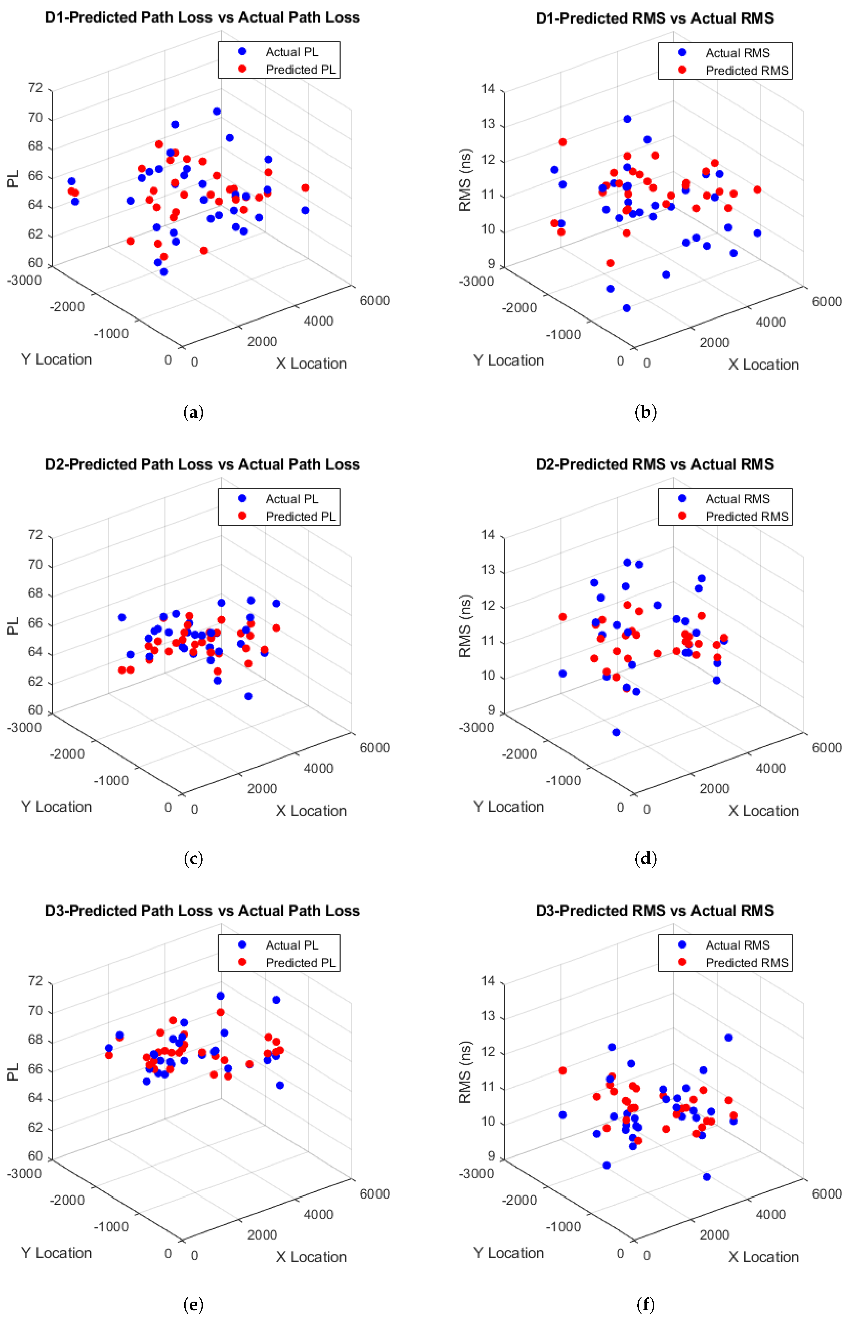
Figure 11.
(a,c,e) estimated path loss and (b,d,f) RMS delay distribution in FTPR.
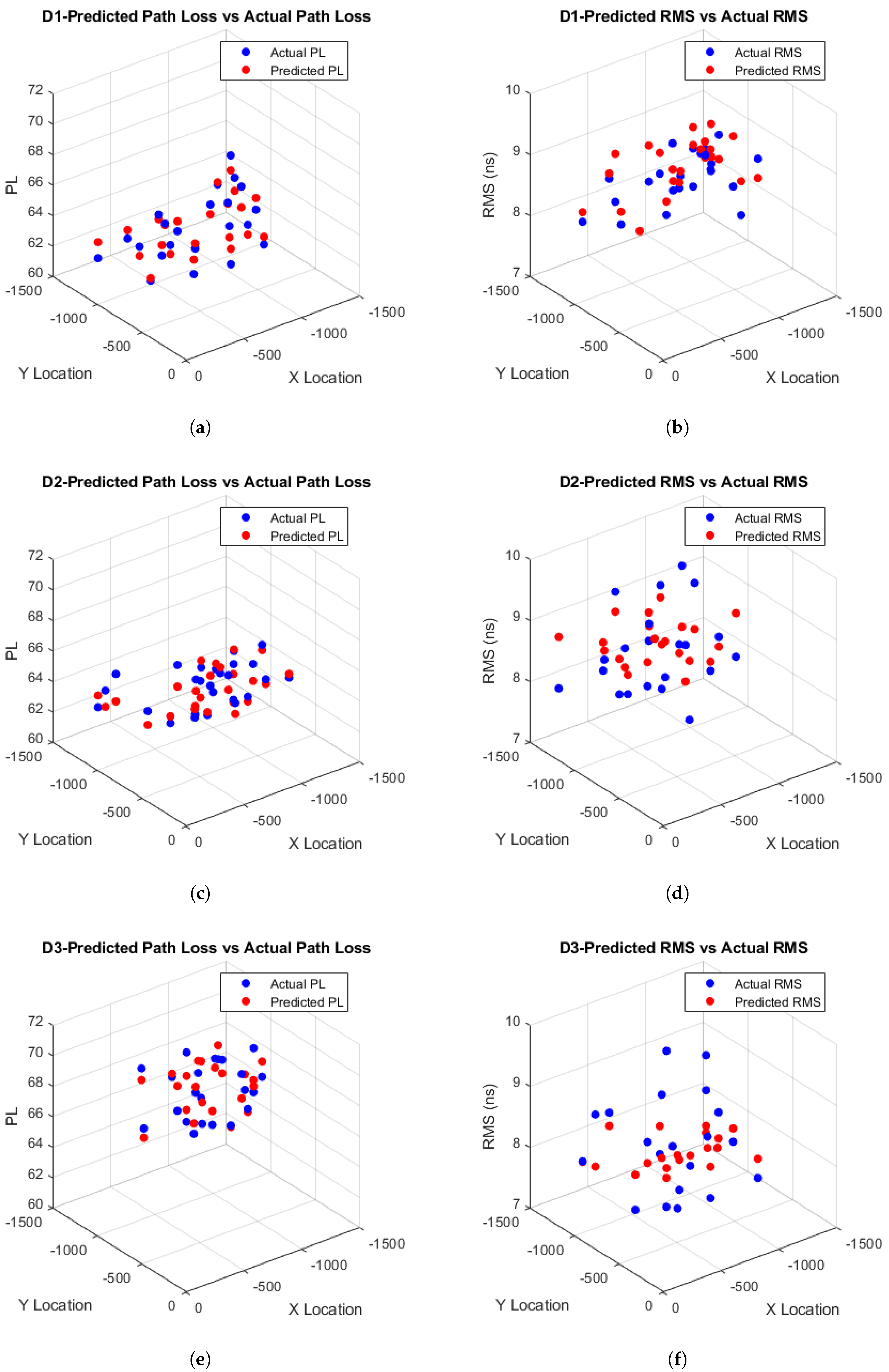

Table 1.
A comparison between 5G and 6G KPIs.
| KPI | 5G | 6G |
|---|---|---|
| Traffic Capacity | 10 Mb/s/m2 | ≈1-10 Gb/s/m3 |
| Data rate: downlink | 20 Gb/s | 1 Tb/s |
| Data rate: uplink | 10 Gb/s | 1 Tb/s |
| Uniform user experience | 50mb/s, 2D | 10Gb/s, 3D |
| Latency (radio interference) | 1 ms | 0.1 ms |
| Jitter | Not Specified | 1 µs |
| Reliability (frame error rate) | 1-10-6 | 1-10-9 |
| Energy/bit | Not Specified | 1 pJ/b |
| Localization precision | 10 cm in 2D | 1 cm in 3D |
Table 2.
Comparative Analysis of ML-Driven Approaches for Link Adaptation in RF Systems.
| Ref | Method | System Model | Proposed ML Model |
|---|---|---|---|
| [27] | K-nearest neighbour method (SL) | Conventionally coded MIMO-OFDM wireless system | - Maps between feature sets and MCS. - Feature space: the SNR of every subcarrier - Large data set is required to learn the function - Increased complexity due to high feature dimensionality. - Ordering subcarriers to minimize feature dimensionality. |
| [28] | Deep Q-learning (RL) | Indoor single-input single-output (SISO) wireless system | - Predicts current CSI and performing link adaptation using outdated CSI. - State space: the most recent transmitted frames are utilized for received signal strength (RSS) measurements - Action space: Several QAM modulation orders - Eliminates quantization errors - Prior environment knowledge not required |
| [29] | Q-learning (RL) | Conventionally coded MIMO-OFDM wireless system (3GPP-LTE standard) | - Identifies the most suitable MCS - State space: Average SNR calculated across all OFDM subcarriers - Action space: Various QAM schemes and coding rates utilized - Quantization-induced throughput degradation - Prior environment knowledge not required |
| [30] | Deep Q-learning (RL) | Wireless system over Rayleigh-faded channel model | - Adaptive modulation using deep Q-network with a trial strategy - State space: Segmentation of the SNR range to establish rate regions. - Action space: Utilizes Gray-coded MPSK schemes for modulation - Eliminates quantization errors - Prior environment knowledge not required |
| [31] | Deep convolutional neural network (SL) | Conventionally coded MIMO-OFDM wireless system | - Establishes relationships between MCS and feature sets - Feature space: Includes SNR for each subcarrier along with noise variance. - Increased complexity due to high feature dimensionality. - Functions without preprocessing steps - Demands significant dataset size for proper learning |
Table 3.
Comparative Analysis of ML-driven Link Adaptation Approaches in AUWC Systems.
| Ref | Method | System Model | Proposed ML Model |
|---|---|---|---|
| [32] | Dyna-q algorithm (RL) | Autonomous underwater vehicle (AUV) | - Predicts the current channel state and adapts modulation based on the predicted current CSI - State space: effective SNR - Action space: QPSK, 8PSK, and BPSK |
| [33] | Hot-booting Q-learning algorithm (RL) | Underwater acoustic | - Dynamically adjusts modulation and coding schemes to optimize QoS by evaluating multiple transmission parameters. - State space: Several transmission factors of present and prior packets - Action space: MFSK and coherent single carrier modulation |
| [34] | Multi-layer perceptron (MLP) network (SL) | Acoustic Internet of underwater things (IoUT) | - Key Challenge: Substantial propagation loss and extreme channel variations - Conventional AMC: Depends on SNR-BER correlation - Link quality parameters: SNR, BER, frequency shift, and delay spread - Demonstrated weak SNR-BER correlation in underwater channels |
| [35] | LSTM-enhanced DQN-based adaptive modulation (RL) | Underwater acoustic | - Key Challenge: Limited observability of acoustic channel - Hybrid RL-LSTM architecture - Improved underwater communication model - Outdated CSI-based link adaptation - State space: Effective SNR derived from preceding time slots - Action space: 8PSK, QPSK, 16QAM, and BPSK - Eliminates quantization errors - Prior environment knowledge not required |
Table 4.
Existing ML-based VLC channel estimation studies.
| Ref | Method | System Model | Machine Learning Improvements |
|---|---|---|---|
| [41] | Extreme Learning Machine (ELM) | Underground mining based VLC system | Improved BER under harsh conditions results in performance close to perfect channel estimation case and outperforms traditional methods. |
| [42] | Artificial Neural Network (ANN)-based ML | Industry channel conditions in a 3D VLP system. | Minimize positioning errors and enhance system accuracy under the smoke channel. |
| [43] | ML-based XGBoost | Indoor VLP system to track the smart trolley’s position | Enhanced deployment speed by reducing training time and maintaining comparable positioning accuracy. |
| [44] | Long Short Term Memory (LSTM) | Indoor VLC channel | Superior BER performance compared to KF, which improves accuracy and system robustness. |
| [45] | Long Short Term Memory (LSTM) | IRS-aided non-linear VLC system | LSTM outperform traditional methods in performance. |
| [46] | LSTM, GRU, and Sparse Autoencoders (SAEs) | Multi-wavelength VLC system with tricolor LED sources | SAEs achieves the best channel modeling performance among other ML algorithms. |
| [47] | Hybrid DNN | Vehicular (V-VLC) and IEEE 802.11p network systems | Outperform traditional models in terms of higher detection accuracy and lower error estimation |
| [48] | DNN, YOLO v3, and Kalman Filter | Indoor VLC system using different modulation techniques. | DNN effectively reduces BER more effectively than KF for all proposed modulation techniques |
| [49] | Random Fourier Features (RFF) based ML | Nonlinear VLC systems | Provides lower training complexity while improving accuracy. |
| [50] | Federated Learning (FL) | Overview VLC networks based on various applications | Reduces data transfer cost, improve privacy and performance. |
Table 5.
LSTM Architecture Parameters.
| Parameters | Specification |
|---|---|
| Optimizer | ADAM |
| Number of iterations | 800 |
| Learning Rate | 0.001 |
| Number of Epochs | 400 |
| Number of Hidden units for LSTM layer | 55 |
Table 6.
System Model and Q-Learning Model Parameters.
| Simulation Parameters | Value |
|---|---|
| Modulation Scheme | M-PAM |
| Min | 0.001 |
| Max Episodes | 500 |
| 0.5 | |
| 0.5 | |
| Responsivity of PDs | 1 |
| 10 dBm | |
Table 7.
Estimated path loss and RMS delay within ICU Ward through different techniques.
| Technique | ICU Ward | |||||
|---|---|---|---|---|---|---|
| RMSE of (dB) | RMSE of (ns) | |||||
| D1 | D2 | D3 | D1 | D2 | D3 | |
| LSTM | 1.6797 | 1.1679 | 1.1464 | 1.0567 | 0.9348 | 0.8784 |
| GRU | 1.7060 | 1.1808 | 1.1774 | 1.0794 | 0.9593 | 0.8840 |
| RNN | 1.7398 | 1.2647 | 1.1785 | 1.0904 | 0.9734 | 0.9039 |
| SVR | 1.8470 | 1.3671 | 1.2654 | 1.1774 | 0.9769 | 0.9107 |
| KNN | 2.3142 | 1.8848 | 1.7834 | 1.8088 | 1.5987 | 1.4401 |
Table 8.
Estimated path loss and RMS delay within FTPR through different techniques.
| Technique | FTPR | |||||
|---|---|---|---|---|---|---|
| RMSE of (dB) | RMSE of (ns) | |||||
| D1 | D2 | D3 | D1 | D2 | D3 | |
| LSTM | 0.7210 | 0.7327 | 1.0652 | 0.5830 | 0.6230 | 0.7657 |
| GRU | 0.7359 | 0.7832 | 1.1480 | 0.6183 | 0.6352 | 0.8555 |
| RNN | 0.7663 | 0.7929 | 1.1886 | 0.6237 | 0.6509 | 0.8509 |
| SVR | 0.7829 | 0.8184 | 1.1762 | 0.6277 | 0.6753 | 0.8834 |
| KNN | 0.9110 | 0.9770 | 1.7908 | 0.8199 | 0.9602 | 1.2166 |
Table 9.
Time complexity of ICU ward.
| Technique | ICU Ward | |||||
|---|---|---|---|---|---|---|
| Execution time of (s) | Execution time of (s) | |||||
| D1 | D2 | D3 | D1 | D2 | D3 | |
| LSTM | 68.051 | 65.854 | 66.229 | 69.946 | 68.786 | 68.948 |
| GRU | 70.197 | 72.190 | 68.958 | 72.711 | 69.671 | 73.468 |
| RNN | 70.368 | 72.578 | 73.488 | 73.018 | 72.917 | 73.787 |
Table 10.
Time Complexity of FTPR.
| Technique | FTPR | |||||
|---|---|---|---|---|---|---|
| Execution time of (s) | Execution time of (s) | |||||
| D1 | D2 | D3 | D1 | D2 | D3 | |
| LSTM | 69.112 | 70.484 | 69.919 | 69.740 | 70.220 | 69.650 |
| GRU | 72.531 | 71.791 | 70.652 | 70.491 | 71.849 | 70.650 |
| RNN | 73.353 | 72.299 | 71.616 | 71.625 | 73.173 | 75.559 |
Disclaimer/Publisher’s Note: The statements, opinions and data contained in all publications are solely those of the individual author(s) and contributor(s) and not of MDPI and/or the editor(s). MDPI and/or the editor(s) disclaim responsibility for any injury to people or property resulting from any ideas, methods, instructions or products referred to in the content. |
© 2025 by the authors. Licensee MDPI, Basel, Switzerland. This article is an open access article distributed under the terms and conditions of the Creative Commons Attribution (CC BY) license (http://creativecommons.org/licenses/by/4.0/).
Copyright: This open access article is published under a Creative Commons CC BY 4.0 license, which permit the free download, distribution, and reuse, provided that the author and preprint are cited in any reuse.


