
Submitted:
28 April 2025
Posted:
29 April 2025
You are already at the latest version
Abstract
Atmospheric corrosion of aluminum alloys is a significant damage case that can occur in many industrial sectors, such as aircraft. To ensure the structural integrity of the affected mechanical structures, structural health monitoring (SHM) is considered a powerful tool. The acoustic emission (AE) method is therefore promising, as it is well suited to localize damage such as corrosion and has already shown to be able to estimate the extent of corrosion. However, the localization and quantification of low-amplitude AE events, such as those caused by atmospheric corrosion of aluminum alloy structures, have not been addressed. The present experimental study investigates the potential of the AE method to localize, quantify, and also characterize the type of atmospheric corrosion of thin-walled aluminum structures by so-called AE-based corrosion imaging, i.e., investigates the potential of AE for full corrosion identification. This AE-based corrosion imaging combines precise AE source localization results from a large number of individual AE events during corrosion to create images for the evaluation of the occurring corrosion. Such AE-based corrosion images can not only be used to localize corrosion, but it is shown that they can assist in estimating the spatial extent of it and also have the potential to characterize corrosion types by considering the temporal evolution of the corrosion images. Through the conducted study, the high potential of the AE method to enable full corrosion identification for future SHM applications for corrosion of aluminum structures is demonstrated.
Keywords:
acoustic emission
; atmospheric corrosion
; localization
; corrosion imaging
; structural health monitoring
1. Introduction
Although aluminum alloys are known for their corrosion resistance, they are not completely immune to degradation in corrosive environments. In various industries such as automotive, transportation, marine, offshore and aviation, aluminium components are often exposed to conditions where complete protection against corrosion is not feasible. Therefore, in aircraft, for example, structural integrity is currently assessed by defined inspection protocols. However, inspections, either visual or supported by non-destructive testing techniques, can be time-consuming and therefore expensive, and may only identify existing corrosion damage of a certain size. Structural health monitoring (SHM) is considered as a powerful tool for earlier and enhanced identification and assessment of ongoing degradation processes such as corrosion [1,2]. SHM is commonly divided into levels that provide different detailed information of a damage. A common distinction is made by the four levels: level 1 detection, level 2 localization, level 3 quantification and level 4 characterization of damage [3]. Among a variety of methods, the acoustic emission (AE) method already showed its excellent suitability for reaching higher level SHM in several applications, including also the monitoring of corrosion [4]. The AE method has already demonstrated its ability for detection (SHM level 1) of different types of aluminum corrosion, predominantly under immersion-like and electro-chemically accerlerated conditions or for stress corrosion cracking (SCC) [1,5,6,7]. In such scenarios, the underlying mechanism causing AE either are artificially amplified or are caused by propagating cracks in loaded mechanical structures. However, it has also been demonstrated that AE is capable of detecting atmospheric corrosion in unloaded aluminum structures. This type of corrosion involves only little amounts of electrolyte, such as small droplets or thin films and the predominant mechanism generating AE is suggested to be low-energy hydrogen bubble activity [5,8]. Atmospheric corrosion frequently occurs under operating conditions in various industrial fields, including plant engineering, transportation, automotive and aviation [9,10,11]. These circumstances result in low signal-to-noise ratio (SNR) AE signals which makes especially higher level SHM of atmospheric corrosion more complex. However, to still enable higher level SHM for atmospheric corrosion of aluminum alloys, recently an AE-based concept for full corrosion identification (i.e., up to SHM level 4) of thin-walled aluminum structures was proposed by the authors. This concept includes precise AE source localization for visualization of corrosion as a key tool for the further quantification and characterization of the corrosion [12]. AE source localization has been a research topic for five decades resulting in a variety of approaches and algorithms. Early work on AE source localization used the triangulation method, which is still a common approach today. Other popular methods include beamforming approaches, modal acoustic emission (algorithms that account for wave physics in thin-walled structures), or more recently also data-driven approaches using machine learning and deep learning models [3,13,14]. Most algorithms that have shown the ability to leading to robust and accurate localization results require information of the time of arrival (TOA), i.e., the time when the AE signal reaches the sensor, which is therefore also a crucial parameter for accurate localization results [15]. However, there are also other sources of localization error. A very comprehensive identification and statistics-based effect quantification analysis was done in [16]. The work used known AE sources on a pressure vessel to quantify the different effects on the localization accuracy. On this thin-walled structure, the scattering of the TOA estimation was found to be the largest. Therefore, to reduce scattering in TOA estimation and thereby enhance localization accuracy, the authors recently proposed a model-based AE source localization algorithm that uses multiple frequency-dependent TOA values instead of a single TOA value [17]. However, no specific research on AE source localization for corrosion of aluminum alloys was found by the authors. Numerous studies, however, have been conducted on the localization and quantification of corrosion of other metals using AE. For example, AE source localization was successfully implemented for localized corrosion of a magnesium alloy plate [18]. Numerous research was done on AE monitoring of steel corrosion reaching also higher SHM levels. In [19] localization of uniform, pitting and crevice corrosion as well as SCC of thin steel plates was shown. In [20], accelerated steel corrosion was investigated, and mass loss estimates were related to the time evolution of different AE features to predict the severity level of the corrosion. And [21] found a linear relationship between cumulative hits and the increasing crack length in SCC. AE monitoring of corrosion in reinforced concrete is another prominent area where successful localization and quantification of the corrosion has been demonstrated. For example, in [22] besides localization of the steel reinforcement corrosion also the amount of corrosion damage in the reinforced concrete was quantified. The cumulative AE energy was used and compared with the mass loss estimate of the steel reinforcement. In addition, AE-based differentiation between pressure or friction of corrosion products and concrete cracking due to corrosion could be shown. In [23] so-called corrosion level estimation in reinforced concrete was investigated by AE. This approach used short term AE monitoring to conduct AE source localization combinded with selective crack length measurements to obtain corrosion level estimates which were validated with mass loss measurements. For comprehensive reviews on corrosion monitoring of reinforced concrete structures it is referred to literature [24,25]. The studies presented above showed localization and also approached quantification of specific corrosion scenarios or damage, with the common feature that precise AE source localization was also an essential part of corrosion quantification. However, approaches to further characterize the type of corrosion and thus to fully identify corrosion by AE have not yet been addressed. During atmospheric corrosion of thin-walled aluminum alloy structures different types of corrosion can occur and interact. All of them require a different severity assessment, so the knowledge of corrosion characteristics especially the corrosion type is essential.
The aim of this paper is to investigate the potential of the AE technique for the characterization of corrosion type and ultimately the full identification of corrosion of aluminum alloys. In particular, localized atmospheric corrosion of thin-walled structures is investigated. To this end, a recently published concept for full corrosion identification is followed [12]. A key tool therefore is the so-called AE-based corrosion imaging, which employs precise AE source localization of the individual corrosion-induced AE events. An experimental study is conducted where localized atmospheric corrosion is induced at four sites on a large AA5754 aluminum alloy plate. Macroscopic photographs of these corrosion sites are taken and processed to extract details about the occurred corrosion. AE monitoring is done by using four piezoelectric wafer active sensors (PWASs) applied to the aluminum alloy plate. A model-based AE source localization algorithm is implemented, particularly intended to be used for low SNR AE signals such as caused by small hydrogen bubbles. The individual localization results are fused to create AE-based corrosion images that visualize the monitored corrosion. Potential corrosion characteristics are identified by analyzing the final state as well as a temporal evolution of these AE-based corrosion images and verified by comparing them to the macroscopic photographs of the corrosion sites.
2. Material and Methods
This section contains a description of the methodology and algorithms used to generate AE-based corrosion images, followed by a specification of the experimental setup and procedure.
2.1. AE-Based Corrosion Imaging
The basis for the generation of AE-based corrosion images are localization results of the individual AE events that occur during the corrosion process. For the corrosion of aluminum, hydrogen bubble activity is considered to be main AE source. When a sufficiently large amount of electrolyte is present, huge numbers of bubbles may occur within a short duration [8]. Plotting the corresponding localization results of such large numbers of AE events naturally results in scattered point clouds as exemplarily shown in Figure 1a. These can be better interpreted by cumulating specific signal features per discrete area at the source location. The proposed AE-based corrosion imaging approach does this by visualizing the localization results in the form of a heat map weighted by the signal energy. Consequently, scattered point clouds are transformed into a spatial distribution of the total measured AE signal energy, which is assumed to represent the spatial distribution of the monitored corrosion, including information on its intensity. In addition to assessing the location of the corrosion, this provides valuable information for corrosion characterization. Figure 1b shows exemplarily the AE-based corrosion image corresponding to the localization results given in Figure 1a. This example shows that the region of the densest localization results can also be seen in the AE-based corrosion image, indicating the general corroded area. However extremely concentrated accumulations of localization results or spots of high AE energy can only be made visible in the AE-based corrosion image. Such localized spots are assumed to indicate very localized corrosion, such as pits.
However, the energy of the measured signals does not directly reflect to the energy at the source position, but is strongly affected by geometric attenuation. For thin-walled structures this geometric attenuation can be approximated by a decrease of the signal amplitude which is inversely proportional to the square root of the propagation distance from the source to the sensor [26,27], i.e., by
where is the peak amplitude of the measured signal from sensor j, the peak amplitude at the source location, and the distance between the source location and the sensor j. Since the signal energy is calculated by the integral of the squared signal amplitude [28], the geometric attenuation for the signal energy can be modelled by an inverse dependence on the propagation distance, i.e., by
where is the signal energy of the measured signal from sensor j and the signal energy at the source location. Therefore Equation 2 is reformulated to obtain values for energy at the source for each sensor . Theoretically this calculated energy at the source should be equal for all sensors. However, due to inaccuracies in the localization, i.e., in , and other uncertainties these obtained values for the energy at the source
differ between the sensors. Therefore the mean value according to
is used for the weighting.
2.2. Model-Based AE Source Localization Algorithm
The proposed AE-based corrosion imaging approach is not bound to a specific AE source localization algorithm. However, the more accurate the individual localization results are, the better the corrosion images become, which can be crucial for corrosion characterization. Therefore a model-based AE source localization algorithm, which reduces uncertainties of state-of the art algorithms is used in the present contribution. This algorithm was already presented in a recent publication of the authors and significant improvements in localization accuracy compared to state-of-the-art triangulation method using Akaike information criterion (AIC) for TOA estimation were shown [17]. In its present form this algorithm considers an infinite thin-walled structure of isotropic and homogeneous materials. The algorithm assumes wave propagation in the form of dispersive guided waves and a predominant excitation of the A0 wave mode, which is typical for AE sources located near the surface of a thin-walled structure [29].
In general, the model-based algorithm is designed as a forward problem. Potential localization results are defined in advance, and an optimization approach is used to find the localization result that best fits the measurement data.
A key aspect of this algorithm is to consider a frequency dependent time of arrival instead of just one single value for TOA. This frequency dependent TOA is a result of the dispersive behavior of the A0 wave mode, which can be obtained in the time-frequency representation of an AE signal calculated by continuous wavelet transform (CWT) [30,31]. This frequency dependency is used to extract multiple values for TOA, i.e., one value per discrete frequency in the spectrogram. Assuming that the distribution of TOA uncertainties follows a Gaussian distribution [16], it is expected that the overall uncertainty will be reduced through averaging when multiple TOAs (one per discrete frequency) are considered. In addition, the frequency-dependent TOA values are determined based on the peak values per discrete frequency in the spectrogram, rather than using a threshold method. Therefore, this approach is also expected to enhance robustness, which is particularly crucial for low SNR AE signals. Another key aspect implemented in the model-based localization algorithm is a coupling of the sensor signals, i.e., the algorithm considers that every sensors receives a signal from exactly the same location and time of origin. This can be considered because the algorithm is designed as a forward problem, i.e., the algorithm always assumes a potential source location and tests how good this location fits to the measurement data. Since also the sensor locations are known, a unique coupling between the sensor signals results. This coupling is expected to further reduce uncertainties and increase robustness of the TOA estimation. However, to get the localization result the following steps are performed. Figure 2 exemplarily illustrates this procedure for the case in which three sensors are used. At the beginning, triangulation using AIC TOA estimation is conducted to get a inital guess for the localization result. Around this inital localization result a quadratic grid of potential localization results is defined, see Figure 2a. Next, for every grid point i the distances from the location of this grid point to the sensor positions are calculated. With this distances the curve of the group velocity of the A0 mode can be transformed into the time-frequency domain for every sensor, see Figure 2b. These transformed curves of the group velocity reflect the frequency dependent TOA for every sensor. Furthermore it also contains the coupling between the sensors, the relative time differences between the transformed dispersion curves are given with this. To find the absolute position in time of the transformed dispersion curve, the curves are shifted together in time until they best fit to the spectrograms of the measured signals. The location of the grid point for which the best overall fit is found, is the final localization result. For a detailed explanation of the algorithm, see [17].
If the best fit lies on a grid point at the edge of the predefined grid, or has a time shift at the upper or lower boundary, this indicates that there may be a better fit, and thus a more accurate localization result. This scenario is used as a further filtering criterion to increase robustness, where all localization results that meet these conditions are excluded from consideration.
2.3. Experimental Setup and Procedure
The experimental setup is shown in Figure 3. The experimental investigation was conducted on a circular plate of AA5754 aluminum alloy with 1 m diameter and 1.46 mm thickness. The edge of the plate was covered with wedge-shaped clay to supress the effect of boundary reflections. Four circular PWAS of 10 mm diameter and 0.5 mm thickness of Pi Ceramic PIC151 material type were adhesively bonded (loctite EA 9466) to thebottom side of the plate, arranged in a quadratic grid of 100 mm × 100 mm, with one sensor positioned in the center of the plate. The first free radial resonance frequency of the PWASs was 194 kHz.
The PWAS were connected via preamplifiers with 40 dB amplification (type Vallen AEP5) to the AE data acquisition system (type Vallen AMSY-6). The atmospheric corrosion was induced on the top side of the plate within the sensor array. Different corrosion sites and scenarios were investigated during the experiment. Generally, corrosion was induced by 0.05 mL droplets of a 50 g/L sodium chloride (NaCl) solution (solution according to DIN EN ISO 9227) at four defined sites and at different times. The sites where corrosion was induced are shown in Figure 4. These corrosion sites were also visually observed by an industrial camera (type IDS UI-3370CP Rev. 2). To observe the different corrosion sites, the camera position was adjusted multiple times throughout the experiment, as only one site could be monitored at a time. In Figure 4 the small circles at sites DLT1, DLT2 and DLT3 with diameters 8.1 mm, 6.7 mm and 7.5 mm represented localized corrosion due to small droplets of the NaCl solution that were placed on the plate. At site CREV a rectangular piece of glass (resistant to corrosion) of dimension 28 mm × 16 mm × 2 mm was placed on the aluminum alloy plate.
Droplets of the NaCl solution were applied to the edges of the glass plate, representing crevice corrosion. However, after the droplets were placed on the plate full evaporation of the solution under room conditions (22-25 °C and 24-36 %RH) was avoided by repeatedly adding approximately 0.03 mL of the NaCl solution or of distilled water, respectively, to the already existing droplets or the edges of the glass piece. This wet phase was followed by a dry phase, i.e. complete evaporation of the droplets under room conditions, leaving NaCl crystals on the plate. After full evaporation, re-wetting of the NaCl crystals was enforced. This was done by an increase of the relative humidity (RH) over the deliquescence relative humidity of NaCl which is 75 %RH [32]. The setup for creating and holding such a high RH is depicted in Figure 5. Three wet sponge cloths were attached to an acrylic glass (PMMA) plate measuring 1.1 m × 1.1 m using adhesive tape. In addition, on the same side of the PMMA plate, distilled water was sprayed onto the plate in a circular band with an inner diameter of about 0.8 m and an outer diameter of about 1 m around the center of the plate. The PMMA plate was placed on the wedge-shaped clay at the edge of the aluminum alloy plate, creating a closed cell of about 10 mm height with high RH around the corrosion sites. To observe RH and temperature inside this cell, a DHT22 sensor was attached on the PMMA plate as well. The chronological sequence of inducing corrosion during the experiment is summarized below.
- A droplet of the NaCl solution was placed at site DLT1. To avoid evaporation, 0.03 mL of the NaCl solution was added hourly to the droplet. After about 9 h from the start no more solution was added. The droplet evaporated. Re-wetting was forced after about 30 h from the placement of the first droplet, the wet state was maintained for about 18 h. Afterwards the evaporation was initiated by removing the PMMA plate from the aluminum alloy plate resulting in exposure to room conditions.
- One droplet was placed at site DLT2 and another one at site DLT3. 0.03 mL of distilled water were added hourly to each droplet to avoid full evaporation. After 8 h no more water was added to allow full evaporation. The re-wetting phase started after 24 h resulting in electrolyte accumulations at sites DLT1, DLT2 and DLT3. This wet state was kept for another 24 h. Afterwards the evaporation was initiated by removing the PMMA plate.
- Several droplets were given to the edges of the glass plate at position CREV. The solution was soaked under the glass plate. Small droplets of distilled water were applied on the edges of the glass plate half-hourly due to the warm and dry conditions (27 °C and 15 %RH) in the laboratory. After about 8 h no more water was added to allow the evaporation. The re-wetting phase started after about 22 h resulting in electrolyte accumulations at sites DLT1, DLT2, DLT3 and around CREV. The wet state was maintained for 24 h. Afterwards final evaporation was initiated by removing the PMMA plate.
2.4. Acoustic Emission Data Acquisition and Pre-Filtering
AE data acquisition (DAQ) was done in hit-based mode and with a sampling frequency MHz. DAQ was started each time after the first electrolyte droplets were placed at the site DLT1, DLT2+DLT3 or at CREV. DAQ was stopped after the subsequent forced evaporations and restarted after the start of the corresponding re-wetting phases. DAQ was briefly interrupted during the times when the PMMA plate was removed and then stopped after the final evaporations. Such periods during the experiment when the DAQ was not running are excluded from the later analysis. For the hit-based DAQ an amplitude threshold of 26 dB with a reference voltage µV [15] was used. The threshold was chosen to be 3 dB above the noise level (proved to suppress small noise outliers), which was approximately constant at 23 dB during the experiment. Prior to the data processing of the proposed model-based AE localization algorithm a pre-filtering procedure was performed to sort out invalid AE events. Invalid AE events were on the one hand assumed to be caused by electrical interferences. Such interferences typically show spike like signals of high amplitude. Furthermore, electrical interferences occur nearly simultaneously at all four sensors. Therefore, the two following criteria were used for AE data cleaning of such interfering signals, (i) if the peak amplitude exceeded 12.5 mV (95 % of the used voltage input range of AMSY-6), or (ii) if threshold based TOA at two or more sensors of an event was smaller or equal the sampling period . This pre-filtering may also eliminate valid AE events that occur e.g., exactly between two sensors. However, since there are large numbers of individual AE events in corrosion, which typically have a natural source location spread, this is not considered relevant in the final AE-based corrosion imaging result. On the other hand, invalid AE events were caused by the repeated manual addition of the NaCl solution. These events resulted in signals with significantly disproportionate energy, which could be easily identified and sorted out.
3. Results and Discussion
The analysis of the measurement data and the implementation of the algorithms described above were done in python. The CWT was calculated using the package ssqueezepy [33] and the required A0 dispersion curves were obtained using the package lambwaves [34].
Visual observations during the experiment confirmed that corrosion occurred only in the areas where the NaCl solution was placed. The forced high RH resulted in the intended deliquescence of the dried NaCl crystals. There were no other accumulations of water or electrolyte on the plate that, e.g., could have been caused by the forced high RH. Further details of the corrosion that occurred are presented in the following sections.
3.1. Environmental Conditions and AE Correlation
Figure 6a shows the environmental conditions, i.e., the temperature and RH during the experiment. The temperature during the experiment varied insignificantly between 22 °C and 25 °C. The periods of time during which a NaCl solution was present on the plate, either by manual addition (see exemplarly Figure 6f) or by deliquescence of NaCl crystals (see exemplarly Figure 6g-j), are indicated by the blue areas with the corresponding descriptions (e.g., ’wet@DLT1’ for manual addition at DLT1, or ’re-wet@DLT1’ for deliquescence at DLT1) in the diagram. The efficiency to force high RH (as presented in Figure 5), is demonstrated by the three rapid increases in the trend of RH (grey dashed curve). No dripping of water droplets from the PMMA plate or the sponge cloths was observed, that could have caused disturbing AE signals. The AE activity at each corrosion site (DLT1, DLT2, DLT3, and CREV) during the experiment is presented separately in Figure 6b-e by the normalized AE hit count and the normalized cumulative AE energy (mean value of the four sensors). The normalization was done by the total AE hit count or the total cumulative AE energy of all four corrosion sites. The assignment of AE hits to the corrosion sites was based on the distances between the corrosion site centers and the localization results obtained by the model-based AE source localization algorithm. Each hit was assigned to its nearest corrosion site (localization results will be discussed in Section 3.2). The periods of time when electrolyte was present on the plate are again indicated in Figure 6b-e by the blue areas and corresponding descriptions in the diagrams. In general, AE activity was detected only during these wetting and re-wetting phases, as indicated by the increases in the cumulative AE activity curves during these time periods. During the remaining phases, i.e., when no liquid electrolyte was present on the plate all these curves stagnate. Except for corrosion site CREV, where after the last re-wetting phase (’re-wet@DLT1/2/3+CREV’) a short increase in the cumulated AE activity can be observed, see Figure 6e. This could be due to slower electrolyte evaporation in the artificial crevice and therefore slightly more AE activity due to corrosion compared to the other three corrosion sites.
In total valid hits were detected during the whole experiment, where were assigned to site DLT1, to site DLT2, to site DLT3, and to site CREV. Corrosion site DLT1 was exposed to electrolyte for the longest time, additionally at this site also the NaCl concentration was higher compared to the other sites, see Section 2.3. It could therefore be expected that most of the AE hits occurred at this site. The sites DLT2 and DLT3 were exposed to the electrolyte for the second longest time, the site CREV for the shortest. The results confirm this for site DLT2, as significantly more hits were detected for this site compared to site CREV. It was expected that site DLT3 would show similar behavior. However, fewer hits were detected at site DLT3 than at site DLT2 and also fewer than at site CREV. The largest increases in AE activity per period when electrolyte was present can always be seen at the corrosion sites that were actually exposed to the electrolyte. However, some AE activity could also be observed in periods when no electrolyte was present at the corresponding site, e.g. during the period ’wet@DLT1’, where slight AE activity was also shown at sites DLT2, DLT3 and CREV. This can be explained by assignments based on inaccurate localization results. In general, for all corrosion sites the trends of the hit count and the cumulative AE energy are very similar, which indicates that in average all hits were of similar energy. Comparison of the wetting phases (e.g., ’wet@DLT2/3’, etc.) and the re-wetting phases (e.g., ’re-wet@DLT1/2/3’) shows that in general more AE activity occurred during re-wetting, i.e. during phases where deliquescence of the NaCl crystals took place. However the re-wetting phases were also of a longer duration. An exception was the first re-wetting phase (’re-wet@DLT1’), where only a few hits (5,020) were detected. During the re-wetting phases, except for ’re-wet@DLT1’, a time delay can be observed between the start of the phase and a noticeable increase in AE activity. This delay can be explained by the time required for deliquescence to produce a sufficient amount of electrolyte, enabling the generation of measurable AE signals due to corrosion [8]. The deliquescence of salt crystals at site DLT2 and during phase ’re-wet@DLT1/2/3’ is exemplary depicted in Figure 6g-j. Slight visual changes due to the deliquescence can be observed after ten minutes (see Figure 6h) and significant deliquescence after one hour (see Figure 6i). In the present example, however, it took about seven hours of deliquescence (see Figure 6j) before a noticeable increase in AE activity occurred.
3.2. AE Source Localization Results
The basis for the proposed AE-based corrosion imaging are AE source localization results of the individual AE events. Therefore, in this subsection the obtained localization results using triangulation approach with AIC for TOA estimation and the proposed model-based AE source localization algorithm are briefly presented. The initially required localization results as starting points for the model-based localization algorithm were calculated by triangulation using the AIC TOA estimator [35]. As expected, the signals were of low amplitude and, as noted above, the identifiable signals were assumed to represent the A0 wave mode due to AE sources at or near the surface of the plate. Therefore, the wave speed of the A0 wave mode was used for triangulation, which was experimentally determined by PLBs to be m/s. The localization results obtained by triangulation are presented in Figure 7a as scatter plot. The spatial resolution for triangulation was set to 0.5 mm × 0.5 mm, which is considered reasonable based on previous research [17]. As expected, the localization of the corrosion shows a large spread. The individual localization results cover the entire plot area, which does not allow a meaningful interpretation. These triangulation results were used as the initially required starting points for the model-based AE source localization algorithm [17]. In the present investigation, a grid of potential localization results around the starting point with a grid resolution of 0.5 mm × 0.5 mm were used for the model-based localization. The coupled time shifting procedure considered 80 time increments ranging from -5.3 µs to +2.7 µs, which is considered reasonable based on previous research [17]. Figure 7b shows the results obtained by the model-based AE source localization algorithm. As described above, the model-based localization algorithm provides an additional filtering criterion to increase its robustness. This criterion discards localization results that could potentially be more accurate if the predefined parameters of the algorithm (grid of potential localization results and time shift range) were different. In present case, applying this criterion resulted in valid localization results, i.e., about 60 % less localization results compared to triangulation. Although this eliminates a large number of AE events, it still leaves a large enough number of AE events to be representative of the corrosion that occurred. Comparison of Figure 7a-b indicate an accuracy improvement of the model-based localization algorithm, by more concentrated and less scattered point clouds of localization results around the sites where the corrosion was triggered (indicated by the white dashed circles and rectangle).
3.3. Corrosion State Imaging
More information can be obtained by visualizing the localization results as heat maps (two-dimensional histogram) weighted by AE energy. The bin size is set to , i.e. the bin size matches the spatial resolution of the localization results. The resulting AE based corrosion images enable visualization of the spatial distribution of the AE activity due to the corrosion, which is not possible for the scatter plots. Figure 8a shows the AE-based corrosion image generated from the results obtained by triangulation using the AIC TOA estimator. Figure 8b shows the AE-based corrosion image generated from the results obtained by the model-based localization algorithm. To highlight AE activity accumulations of lower intensity, a specific scaling method is applied to the corrosion images in Figure 8. For bins with values up to of the integrated energy represented by the heat map, a linear scaling is used. For bins with higher values, a logarithmic scaling is applied. In the present analysis, the scaling is realized by using a symmetric logarithmic scale [36].
Comparison of the two corrosion images in Figure 8 shows that using the model-based localization algorithm regions of highest AE activity are of less scatter and move more towards the actual corrosion sites, i.e., indicating the improvement in robustness and localization accuracy. For site DLT1 Figure 8b shows a concentrated accumulation mainly inside and below the dashed circle, which fits well with the observed corrosion (see macroscopic photograph in Figure 9a). In contrast, Figure 8a shows an accumulation at the left edge of the circle, which is less consistent with the observed corrosion. Moreover, a distinct accumulation is also observed approximately 17 mm to the left. No NaCl solution was placed at this location, and no corrosion could be identified through visual inspection, i.e., the corrosion image based on triangulation indicated a non-existent corrosion at this location. More distinct and accurate corrosion imaging results are also obtained at the other corrosion sites when the model-based localization algorithm is used instead of triangulation. For sites DLT2 and DLT3, Figure 8b shows small but concentrated accumulations inside the white dashed circles, while in Figure 8a these accumulations are less intense, more scattered, and located outside the white dashed circles. For corrosion site CREV Figure 8b shows a small accumulation of very low intensity near the top right corner of the white dashed rectangle. However, in Figure 8a such a accumulation is not visible near this corrosion site. In general, both corrosion images show that most of the AE activity originated from site DLT1, less from sites DLT2 and DLT3, and hardly any activity at or near site CREV. However, Figure 6 shows that more AE activity was detected at site CREV than at site DLT3. A closer look at site CREV revealed that the detected AE activity was more spatially scattered compared to site DLT3 and therefore appears less in the corrosion images.
To verify the AE-based corrosion images with respect to the occured corrosion, macroscopic photographs of the sites DLT1-3 and CREV were taken at the end of the experiment. Before these photographs were taken, the corrosion sites were first rinsed with distilled water and then cleaned with isopropyl alcohol. In order to remove the remaining corrosion products, the corrosion sites were etched with nitric acid according to standard DIN EN ISO 8407. The captured photographs of the cleaned plate surface of sites DLT1-3 and CREV are shown in Figure 9. In addition, Figure 9 shows the corresponding detail views of sites DLT1-3 and CREV of the AE-based corrosion image given in Figure 8b. To better highlight the AE activity per corrosion site, the AE activity in the detail views is normalized by the cumulative AE energy of the corresponding corrosion site. Furthermore, a linear scaling is applied to the corrosion images in Figure 9. The macroscopic photographs clearly show uniform areal corrosion by the uniform discoloring in the areas where the droplets of NaCl solutions were initially placed (DLT1-3) and in the rectangular area where the glass plate was placed (CREV). They also show pitting corrosion by numerous pits of different sizes both within and outside these areas of uniform areal corrosion. To better highlight the occured corrosion in the photograph, the photgraph is additionally converted from red green blue (RGB) color system into the hue saturation brightness (HSB) color system, followed by thresholding. This method is commonly used for visual analysis of corroded surfaces [37,38]. It turned out that, in particular, the thresholded hue channel effectively highlights the uniform areal corrosion, while the thresholded brightness channel highlights pitting corrosion. The used thresholding method sets an upper and a lower threshold for each, the 8-bit hue and the 8-bit brightness channel. In the used analysis the lower threshold was set to 0 and the upper threshold was set to include a certain percentage of the corresponding pixel histogram of the channel. For the hue channel, this percentage value was set to be 30% and for the brightness channel this value was set to be 1%.
In the detail views of the AE-based corrosion image the sites where the NaCl droplets were initally placed and the area where the glass plate was placed are again marked by the white dashed circles and the white dashed rectangle. Figure 9a represents site DLT1. A large part of the detected AE activity is inside the white dashed circle, which correlates well with the uniform areal corrosion, but also with the pitting that can be seen in the macroscopic photograph and the thresholded brightness channel. However another large part of the detected AE activity is located at the bottom edge and also outside of the white dashed circle. This accumulation of AE activity also includes the spot of highest spatial AE intensity for the corrosion site DLT1. The macroscopic photograph and the thresholded brightness channel show significant pitting corrosion in this region. However, less uniform areal corrosion occured in this region as indicated by the thresholded hue channel. In this area on the aluminum alloy plate, the droplet gradually expanded beyond its circular shape beginning during the second drying phase (hours 42-46 in Figure 6). During the subsequent re-wetting and drying phases, this area expanded even more. Therefore, corrosion could also occur in these areas where a corrosive solution was never applied. It is assumed, that the higher amount of NaCl at this site (compared to sites DLT2-3) absorbed more water during the deliquescence process. As a result, it was no longer possible to concentrate this larger amount of NaCl solution into a single droplet. Figure 10 shows the result of this behavior at the end of the experiment, that is, before the cleaning procedure to remove the NaCl crystals and the corrosion products.
Figure 9b represents site DLT2. Inside the left half of the white dashed circle of the AE-based corrosion image, uniformly scattered AE activity is found. The most intense AE activity is found in the right half of the circle with the most intense spot located around the bottom right edge of the circle. Similar behavior can be seen in the macroscopic photograph and the thresholded hue and brightness channel of this corrosion site. Uniform areal corrosion is given by the circular area where the droplet of the NaCl solution was initially placed. In addition, most of the pitting is found in the region around the bottom right edge of the circular area, but less pitting is seen in the other regions of this corrosion site. These results are also supported by the visual observation of this corrosion site during the experiment. During the ’re-wet @ DLT1/2/3’ phase, the deliquescence of the NaCl crystals occurred predominantly in the right half of the circular area where the droplet was initially placed, see exemplary Figure 6j. For corrosion site DLT2, also most of the AE activity was detected during this re-wetting phase, see Figure 6c. These observations confirm the large accumulation of intense AE activity in the AE-based corrosion image of Figure 9b. Figure 9c represents site DLT3. The corrosion image of this site is dominated by a very localized hotspot located at the bottom left edge of the white dashed circle. Uniformly scattered AE activity is found inside the white dashed circle, from the above described hotspot until the right edge of the white dashed circle. The macroscopic photograph shows a large pit at nearly the same position as indicated by the hotspot in the AE-based corrosion image. The macroscopic photograph and the thresholded brightness channel show areas of numerous small pits where scattered AE activity is found in the corrosion image. Figure 9d represents site CREV. In general very scattered AE activity is found for this corrosion site. However, the region of most intense AE activity is not located inside the white dashed rectangle but more outside this rectangle, that represents the area where the glass plate was placed. The most AE activity is given by an accumulation near the top right corner of this rectangle. The macroscopic photograph and the thresholded hue and brightness channel show slight uniform areal corrosion in a rectangular shape, and in addition next to its top right corner. Pitting can also be seen in this region. This region fits well with the accumulation of AE activity in the corresponding AE-based corrosion image. The thresholded brightness channel also indicates pitting along the bottom edge of the rectangular corroded area. However, a closer look at the macroscopic image shows no significant pitting in this area, so this indication is considered a misinterpretation. In general, the macroscopic photographs and the thresholded hue and brightness channel show less corrosion at site CREV than at the other corrosion sites.
All these results have in common that the most intense AE activity spatially correlates with regions where pitting occurred. Moreover, in Figure 9c, it was also found that a very localized AE hotspot correlates very well with a significant pit in the macroscopic photograph. However, this is not always the case. There are large or significant pits that cannot be clearly assigned to hotspots of AE activity. Possible reasons for this could be systematic errors in the experimental setup, such as imperfect sensor placement. Furthermore, it is expected that repeated AE events from the same location, e.g., AE events from the same pit, result in similar AE signals. Therefore, it is expected that the localization error will be similar. This means that the localization error can vary from pit to pit. Consequently, this could mean that some pits were detected by AE but not clearly shown in the AE-based corrosion image, e.g., because the corresponding hotspots of AE activity overlap in the corrosion image. It should also be mentioned that the overall localization accuracy obtained in the present experiment is already very good. The results in Figure 9 show that the general corrosion sites are very well identified, and even some localized hotspots within these sites (diameters from to for DLT1-3, and for CREV) can be found with with small spatial deviations in the low single-digit millimeter range.
The agreements found above between the observed corrosion and the AE-based corrosion images highlight the applicability of the proposed corrosion imaging approach. Specifically, the high accuracy of the model-based localization algorithm is of high value, as it enables detailed images of corrosion sites. This enables to accurately estimate the spatial extent of corrosion and also may allow to characterize different forms of corrosion, such as pitting corrosion and uniform areal corrosion for the present investigation.
3.4. Corrosion Evolution Imaging
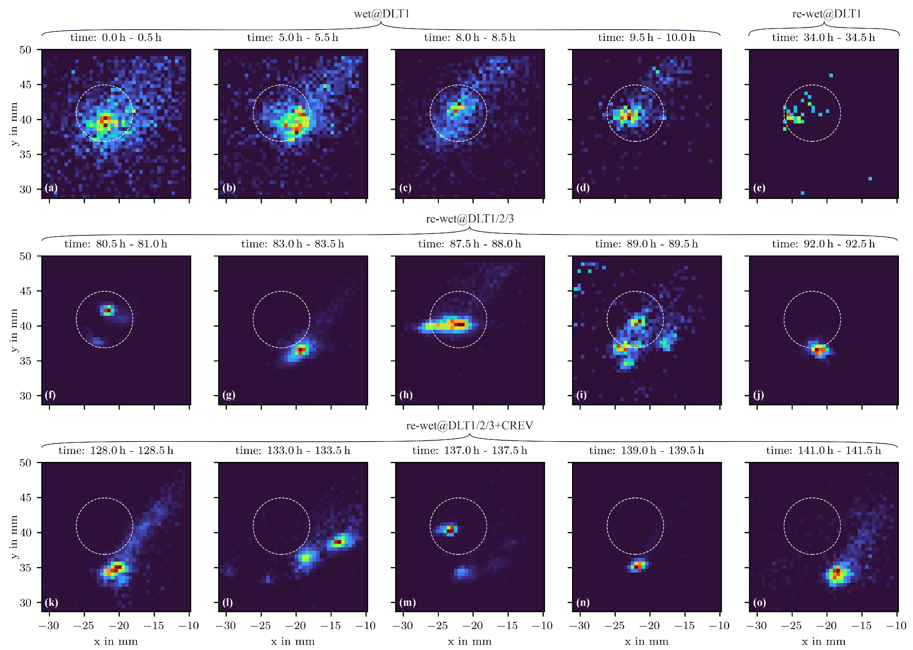
The results presented above describe the final corrosion state after the entire experiment, i.e. a cumulative result after approximately 150 hours. However, the proposed corrosion imaging approach also allows the investigation of the temporal evolution of the corrosion that occurred by evaluating not only one, but multiple and shorter consecutive time windows of the detected and localized AE activity. This provides additional information about the corrosion occurred, and thus could make a valuable contribution to corrosion identification. This investigation yielded very similar results for all corrosion sites. Exemplary results of this corrosion evolution imaging are presented for the AE activity measured at corrosion site DLT1. For this purpose, a video was created with consecutive corrosion images, each showing the AE activity in a 30 minute time window. This duration proved to be a sensible and practicable value for visualizing the temporal evolution of AE-based corrosion images. The heat maps behind the corrosion images were normalized by the cumulative energy of hits that occurred during the corresponding 30 minute time window. Figure 11 shows representative video frames, i.e., corrosion images with the corresponding time window information. Figure 11a-d show corrosion images during phase ’wet@DLT1’, i.e., when a droplet was placed and maintained at site DLT1. These short time corrosion images show very scattered AE activity at and around the white dashed circle that represents the initially wetted surface. However, the most intense regions of these scattered AE activity lies always inside this circle. Figure 11e shows a corrosion image during the first re-wetting phase (’re-wet@DLT1’). This representative corrosion image shows hardly any AE activity, as it was already indicated by the cumulative AE trends of site DLT1 in Figure 6b. Figure 11f-j show corrosion images during the second re-wetting phase (’re-wet@DLT1/2/3’). During this phase a lot of AE activity was measured. The resulting corrosion images show spatially very concentrated and hardly scattered accumulations. These concentrated accumulations occurred at many different positions within the white dashed circle and also outside the circle close to the bottom edge. The accumulations outside the circle and close to the bottom edge fit very well in space and time with the visual observations during the experiment. During this re-wetting phase, electrolyte was formed at these areas for the first time, allowing corrosion to take place. These concentrated accumulations of AE activity differ significantly from the scattered AE activity of Figure 11a-d, i.e., also suggesting different corrosion characteristics or corrosion types.
Figure 11k-o show corrosion images during the third and last re-wetting phase (’re-wet@DLT1/2/3 +CREV’). Very concentrated accumulations of AE activity at different positions are shown again. However, during this phase almost all of these accumulations were located outside the white dashed circle, near the bottom right edge. Again these accumulations correlate very well with the visual observations during the experiment. The deliquescence of the NaCl crystals began during this re-wetting phase at this area and also in general more electrolyte was formed at this area outside the circle compared to the area within the circle.
Two different corrosion characteristics are suggested by the investigation of the temporal evolution of the AE-based corrosion images. First, at the beginning, spatially very scattered AE activity can be observed, predominantly within the white dashed circle, see Figure 11a-d. It is suggested that these corrosion images represent general corrosion that took place uniformly distributed within the white dashed circle. Second, corrosion images obtained in later phases showed spatially concentrated accumulations in many different positions. These accumulations suggest localized corrosion, such as pitting, and may even indicate the formation or growth of individual pits. These suggestions are supported by the macroscopic photograph and the thresholded hue and brightness channel of Figure 9a. As described above, these images show uniform areal corrosion at the circular surface where the droplet of NaCl solution was initially placed, and pitting corrosion in the same region, but also below and to the right of this circular region. These results demonstrate the ability of the AE-based corrosion imaging approach to support corrosion type characterization and are therefore considered to be a valuable contribution to full corrosion identification by AE.
4. Conclusions
This experimental study investigates the potential of so-called AE-based corrosion imaging for quantification (SHM level 3) and type characterization (SHM level 4) of atmospheric corrosion in thin-walled aluminum alloy structures. The presented AE-based corrosion imaging approach combines a large number of AE source localization results caused by corrosion to a heat map weighted by the AE energy to enable visualization and evaluation of corrosion. An area of 100 mm × 100 mm on a large AA5754 aluminum alloy plate was monitored by AE using four PWASs. Localized atmospheric corrosion was induced at four positions within this area by droplets of a 50 g/L NaCl solution, resulting in corrosion sites ranging in size from 6.7ṁm to 28ṁm. AE source localization was performed using a model-based algorithm, resulting in significant improvements over localization using the state-of-the-art triangulation method based on AIC TOA estimation. In the AE-based corrosion image, especially the localized corrosion sites caused by single NaCl solution droplets were clearly identified, showing very good spatial agreement with the actual corroded areas on the plate. The AE-based corrosion images were verified by macroscopic photographs of the occurred corrosion on the plate. In order to better highlight the corrosion, these photographs were also transformed and analyzed in the HSB color system. Detail views of the AE-based corrosion image showed that the general corroded areas on the plate were well represented by scattered but less intense AE activity. However, the most intense accumulations of AE activity correlated well with regions where predominantly pitting occurred, with only small spatial deviations in the single-digit-millimeter range. The AE-based corrosion imaging approach also allows for evaluation of the temporal evolution of corrosion by generating consecutive corrosion images based on AE data of short-duration time windows. Initially, more spatially scattered AE activity was observed, indicating uniform areal corrosion. In later phases, various small localized hotspots of AE activity appeared, suggesting pitting corrosion. The macroscopic photographs show these two corrosion types as well with very good spatial agreements to the described AE activity in the AE-based corrosion images.
To conclude, it was shown that AE-based corrosion imaging accurately localized (SHM level 2) atmospheric corrosion of a thin-walled aluminum alloy structure. Moreover, it was shown that it can assist quantification (SHM level 3) of corrosion by estimating the general corroded area. Finally, the evaluation of the temporal evolution of AE-based corrosion images highlights certain corrosion characteristics, such as temporal corrosion hotspots. This suggests that AE-based corrosion imaging may also enable corrosion type characterization (SHM level 4). All these results clearly demonstrate the potential of AE-based corrosion imaging as a key tool for future identification of corrosion of mechanical structures for SHM applications.
In future research, noisier environments shall be considered, e.g., through a standardized salt spray chamber test, to validate the robustness of the approach. Quantification of corrosion by AE will further be investigated by comparison of mass loss measurements during corrosion with AE signal characteristics and features. Characterization of the corrosion types will be enhanced by considering a-priori knowledge such as geometry and material of the investigated mechanical structure.
References
- P. D. Mangalgiri, Corrosion issues in structural health monitoring of aircraft, ISSS Journal of Micro and Smart Systems 8 (1) (2019) 49–78. [CrossRef]
- R. F. Wright, P. Lu, J. Devkota, F. Lu, M. Ziomek-Moroz, P. R. Ohodnicki, Corrosion Sensors for Structural Health Monitoring of Oil and Natural Gas Infrastructure: A Review, Sensors 19 (18) (2019) 3964. [CrossRef]
- M. G. R. Sause, E. Jasiūnienė (Eds.), Structural Health Monitoring Damage Detection Systems for Aerospace, Springer Aerospace Technology, Springer International Publishing, Cham, 2021. doi: 10.1007/978-3-030-72192-3.
- M. Wevers, K. Lambrighs, Applications of Acoustic Emission for SHM: A Review, in: Encyclopedia of Structural Health Monitoring, John Wiley & Sons, Ltd, 2009. [CrossRef]
- F. Bellenger, H. Mazille, H. Idrissi, Use of acoustic emission technique for the early detection of aluminum alloys exfoliation corrosion, NDT & E International 35 (6) (2002) 385–392. [CrossRef]
- C. Abarkane, A. M. Florez-Tapia, J. Odriozola, A. Artetxe, M. Lekka, E. García-Lecina, H. J. Grande, J. M. Vega, Acoustic emission as a reliable technique for filiform corrosion monitoring on coated AA7075-T6: Tailored data processing, Corrosion Science 214 (2023) 110964. [CrossRef]
- L. Calabrese, E. Proverbio, A Review on the Applications of Acoustic Emission Technique in the Study of Stress Corrosion Cracking, Corrosion and Materials Degradation 2 (1) (2021) 1–30. [CrossRef]
- T. Erlinger, C. Kralovec, M. Schagerl, Monitoring of Atmospheric Corrosion of Aircraft Aluminum Alloy AA2024 by Acoustic Emission Measurements, Applied Sciences 13 (1) (2023) 370. [CrossRef]
- F. Ostermann, Anwendungstechnologie Aluminium, Springer Berlin Heidelberg, Berlin, Heidelberg, 2014. [CrossRef]
- C. Vargel, Corrosion of Aluminium, 2nd Edition, Elsevier, Amsterdam, 2020. [CrossRef]
- A. du Plessis, Studies on Atmospheric Corrosion Processes in AA2024, Ph.D. thesis, University of Birmingham (2015).https://etheses.bham.ac.uk/id/eprint/5642/5642.
- T. Erlinger, C. Kralovec, M. Schagerl, Acoustic emission-based structural health monitoring concept for corrosion of aluminum aircraft structures, e-Journal of Nondestructive Testing 28 (1) (2023). [CrossRef]
- T. Kundu, Acoustic source localization, Ultrasonics 54 (1) (2014) 25–38. [CrossRef]
- F. Hassan, A. K. B. Mahmood, N. Yahya, A. Saboor, M. Z. Abbas, Z. Khan, M. Rimsan, State-of-the-Art Review on the Acoustic Emission Source Localization Techniques, IEEE Access 9 (2021) 101246–101266. [CrossRef]
- C. U. Grosse, M. Ohtsu, D. G. Aggelis, T. Shiotani (Eds.), Acoustic Emission Testing: Basics for Research – Applications in Engineering, Springer Tracts in Civil Engineering, Springer International Publishing, Cham, 2022. [CrossRef]
- S. Kalafat, M. G. Sause, Acoustic emission source localization by artificial neural networks, Structural Health Monitoring 14 (6) (2015) 633–647. [CrossRef]
- T. Erlinger, C. Kralovec, C. Humer, M. Schagerl, Impact of Model Knowledge on Acoustic Emission Source Localization Accuracy, e-Journal of Nondestructive Testing 29 (2024). [CrossRef]
- M. Mandel, M. Fritzsche, S. Henschel, L. Krüger, Lamb wave-based corrosion source location on a plate of magnesium alloy WZ73 using the acoustic emission technique, Corrosion Communications 13 (2024) 60–67. [CrossRef]
- C. Jomdecha, A. Prateepasen, P. Kaewtrakulpong, Study on source location using an acoustic emission system for various corrosion types, NDT & E International 40 (8) (2007) 584–593. [CrossRef]
- M. F. Sheikh, K. Kamal, F. Rafique, S. Sabir, H. Zaheer, K. Khan, Corrosion detection and severity level prediction using acoustic emission and machine learning based approach, Ain Shams Engineering Journal 12 (4) (2021) 3891–3903. [CrossRef]
- Z. Zhang, Z. Zhang, J. Tan, X. Wu, Quantitatively related acoustic emission signal with stress corrosion crack growth rate of sensitized 304 stainless steel in high-temperature water, Corrosion Science 157 (2019) 79–86. [CrossRef]
- C. Van Steen, L. Pahlavan, M. Wevers, E. Verstrynge, Localisation and characterisation of corrosion damage in reinforced concrete by means of acoustic emission and X-ray computed tomography, Construction and Building Materials 197 (2019) 21–29. [CrossRef]
- E. Vandecruys, C. Martens, C. Van Steen, G. Lombaert, E. Verstrynge, Corrosion level estimation in reinforced concrete beams by acoustic emission sensing and selective crack measurements, Structural Concrete n/a (n/a) (2024). [CrossRef]
- A. Zaki, H. K. Chai, D. G. Aggelis, N. Alver, Non-Destructive Evaluation for Corrosion Monitoring in Concrete: A Review and Capability of Acoustic Emission Technique, Sensors 15 (8) (2015) 19069–19101. [CrossRef]
- E. Verstrynge, C. Van Steen, E. Vandecruys, M. Wevers, Steel corrosion damage monitoring in reinforced concrete structures with the acoustic emission technique: A review, Construction and Building Materials 349 (2022) 128732. [CrossRef]
- K. Asamene, L. Hudson, M. Sundaresan, Influence of attenuation on acoustic emission signals in carbon fiber reinforced polymer panels, Ultrasonics 59 (2015) 86–93. [CrossRef]
- K. Ono, Review on Structural Health Evaluation with Acoustic Emission, Applied Sciences 8 (6) (2018) 958. [CrossRef]
- D. G. Aggelis, M. G. R. Sause, P. Packo, R. Pullin, S. Grigg, T. Kek, Y.-K. Lai, Acoustic Emission, in: M. G. R. Sause, E. Jasiūnienė (Eds.), Structural Health Monitoring Damage Detection Systems for Aerospace, Springer Aerospace Technology, Springer International Publishing, Cham, 2021, pp. 175–217. doi: 10.1007/978-3-030-72192-3_7.
- M. A. Hamstad, On Lamb Modes As a Function Of Acoustic Emission Source Rise Time, Journal of Acoustic Emission (28) (2010) 41–58.
- J. Jiao, C. He, B. Wu, R. Fei, X. Wang, Application of wavelet transform on modal acoustic emission source location in thin plates with one sensor, International Journal of Pressure Vessels and Piping 81 (5) (2004) 427–431. [CrossRef]
- F. Ciampa, M. Meo, Acoustic emission source localization and velocity determination of the fundamental mode A0 using wavelet analysis and a Newton-based optimization technique, Smart Materials and Structures 19 (4) (2010) 045027. [CrossRef]
- E. Schindelholz, R. G. Kelly, Wetting phenomena and time of wetness in atmospheric corrosion: A review, Corrosion Reviews 30 (5-6) (2012) 135–170. [CrossRef]
- J. Muradeli, Ssqueezepy, GitHub repository, https://github.com/OverLordGoldDragon/ssqueezepy/ (2020). [CrossRef]
- F. Rotea, Lambwaves, GitHub repository, https://github.com/franciscorotea/Lamb-Wave-Dispersion (2020).
- J. H. Kurz, C. U. Grosse, H.-W. Reinhardt, Strategies for reliable automatic onset time picking of acoustic emissions and of ultrasound signals in concrete, Ultrasonics 43 (7) (2005) 538–546. [CrossRef]
- Matplotlib, Matplotlib.colors.SymLogNorm (2025). https://matplotlib.org/stable/api/_as_gen/matplotlib. colors.SymLogNorm.html (accessed: 22 April 2025).
- V. Bonamigo Moreira, A. Krummenauer, J. Zoppas Ferreira, H. M. Veit, E. Armelin, A. Meneguzzi, "Computational image analysis as an alternative tool for the evaluation of corrosion in salt spray test ", Studia Universitatis, Babes-Bolyai Chemia 65 (3) (2020) 45–61. [CrossRef]
- I. Ivasenko, V. Chervatyuk, Detection of Rust Defects of Protective Coatings Based on HSV Color Model, in: 2019 IEEE 2nd Ukraine Conference on Electrical and Computer Engineering (UKRCON), 2019, pp. 1143–1146. [CrossRef]
Figure 1.
Illustration of the AE-based corrosion imaging. (a) Scatter plot of localization results only roughly indicates the potential corroded, (b) the corresponding AE-based corrosion image also makes localized corrosion spots visible.
Figure 1.
Illustration of the AE-based corrosion imaging. (a) Scatter plot of localization results only roughly indicates the potential corroded, (b) the corresponding AE-based corrosion image also makes localized corrosion spots visible.
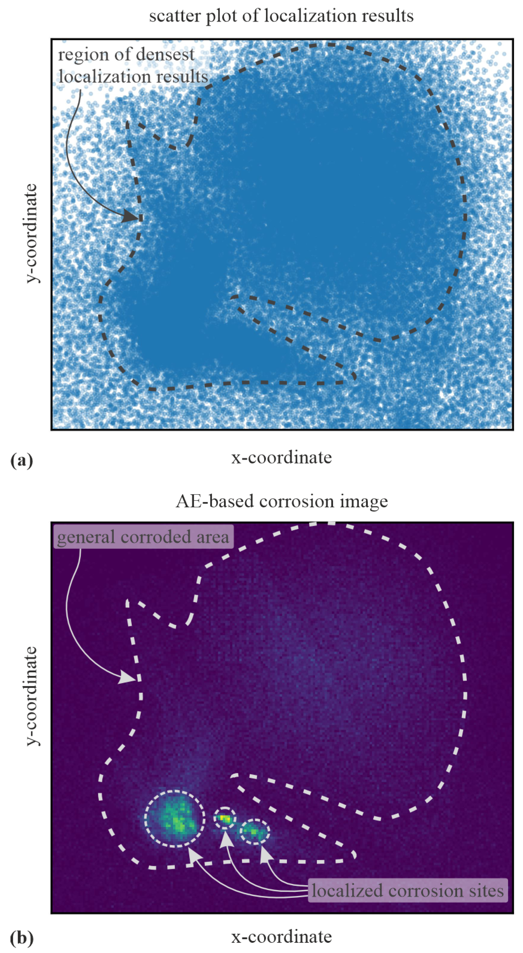
Figure 2.
Explanation of the model-based AE source localization algorithm. (a) Exemplary thin-walled structure with three sensors ch1…ch3, and predefined grid points i as potential localization results. (b) Procedure to find the best common fit of the transformed dispersion curves to the spectrograms resulting from the measurement data.
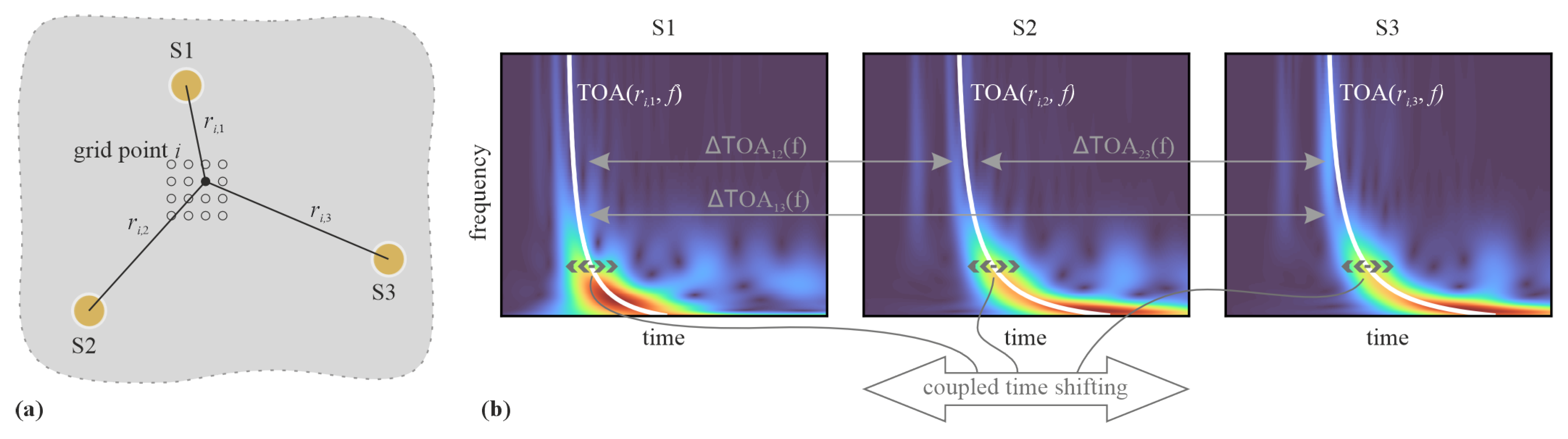
Figure 3.
Experimental setup for the investigation. Wedge-shaped clay is put on the edge of the circular AA5754 plate. AE monitoring is conducted by four PWAS adhesively bonded to the underside of the plate. In addition, video recordings and measurements of temperature and relative humidity are made.
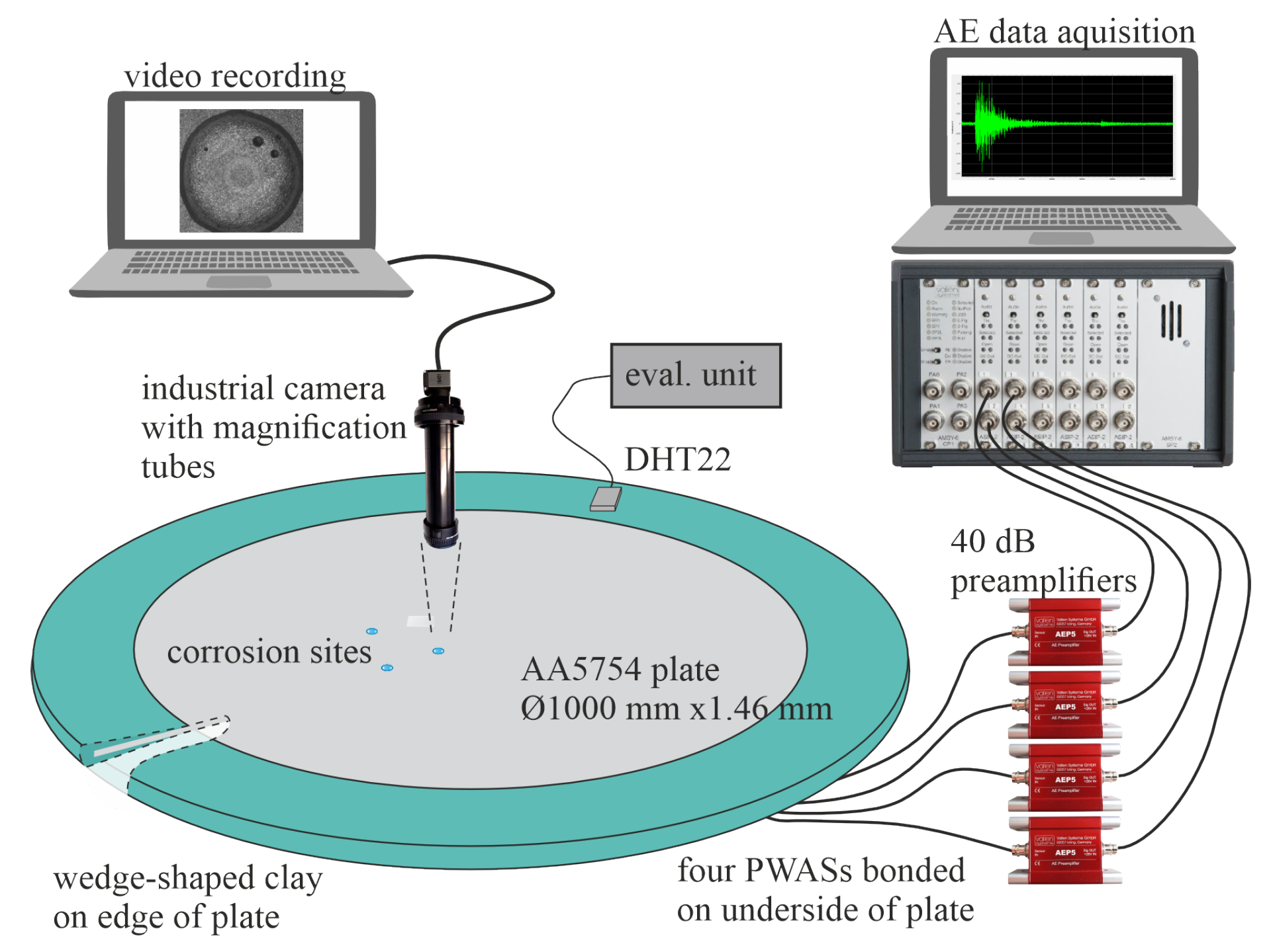
Figure 4.
Positions of corrosion sites DLT1, DLT2, DLT3 and CREV on top side of plate (dimensions in mm). The sensor S1-S4 are placed on the underside of the plate in a quadratic arrangement with side length 100 mm with S3 in the center of the plate.
Figure 4.
Positions of corrosion sites DLT1, DLT2, DLT3 and CREV on top side of plate (dimensions in mm). The sensor S1-S4 are placed on the underside of the plate in a quadratic arrangement with side length 100 mm with S3 in the center of the plate.
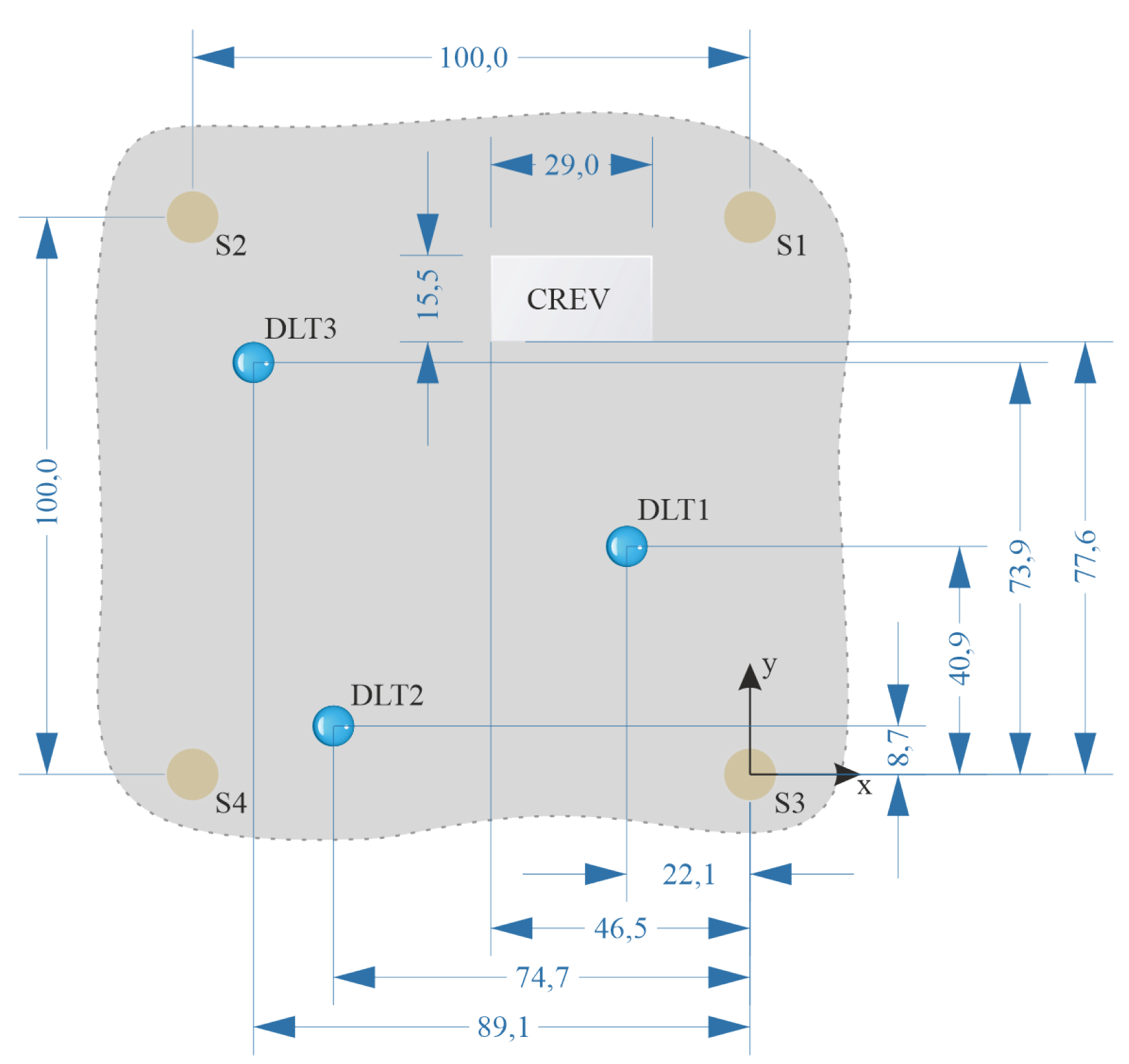
Figure 5.
A PMMA plate with three wet sponge cloths on its underside is placed on top of the wedge-shaped clay, creating an approximately 10 mm high closed cell of high RH. The DHT22 sensor is also attached to the underside of the PMMA plate. Neither the DHT22 nor the sponge cloths are in contact with the aluminum surface.
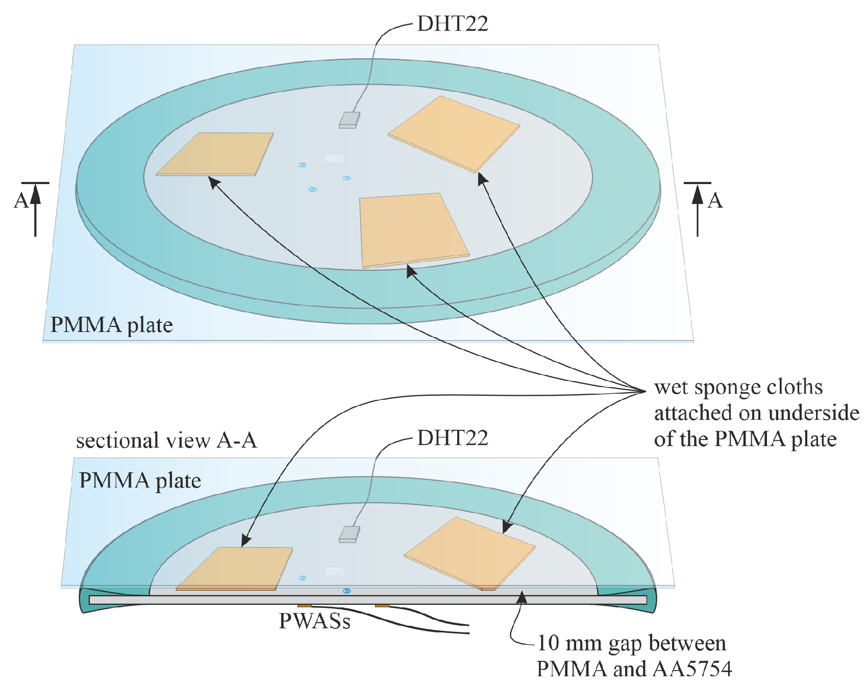
Figure 6.
Correlation between the phases when electrolyte was present on the aluminum plate and the AE activity detected. (a) Trends of the environmental conditions during the experiment, (b-e) normalized AE hits and cumulative AE energy of the corrosion sites DLT1, DLT2, DLT3, and CREV, and (f-j) exemplary pictures of site DLT2 at different times during the experiment.
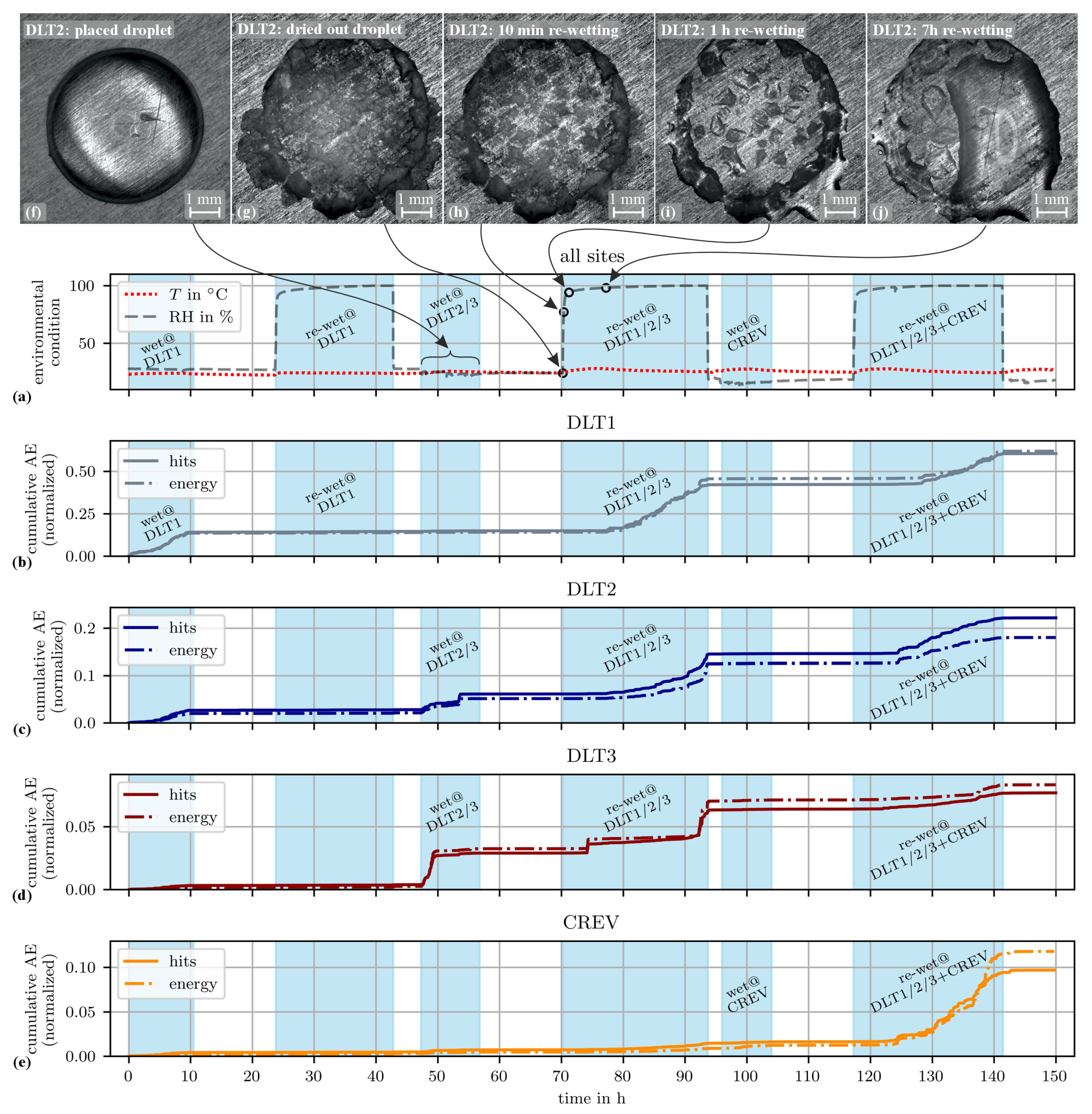
Figure 7.
Localization results (a) obtained by triangulation using AIC TOA estimation, and (b) obtained by the model-based AE source localization algorithm.
Figure 7.
Localization results (a) obtained by triangulation using AIC TOA estimation, and (b) obtained by the model-based AE source localization algorithm.
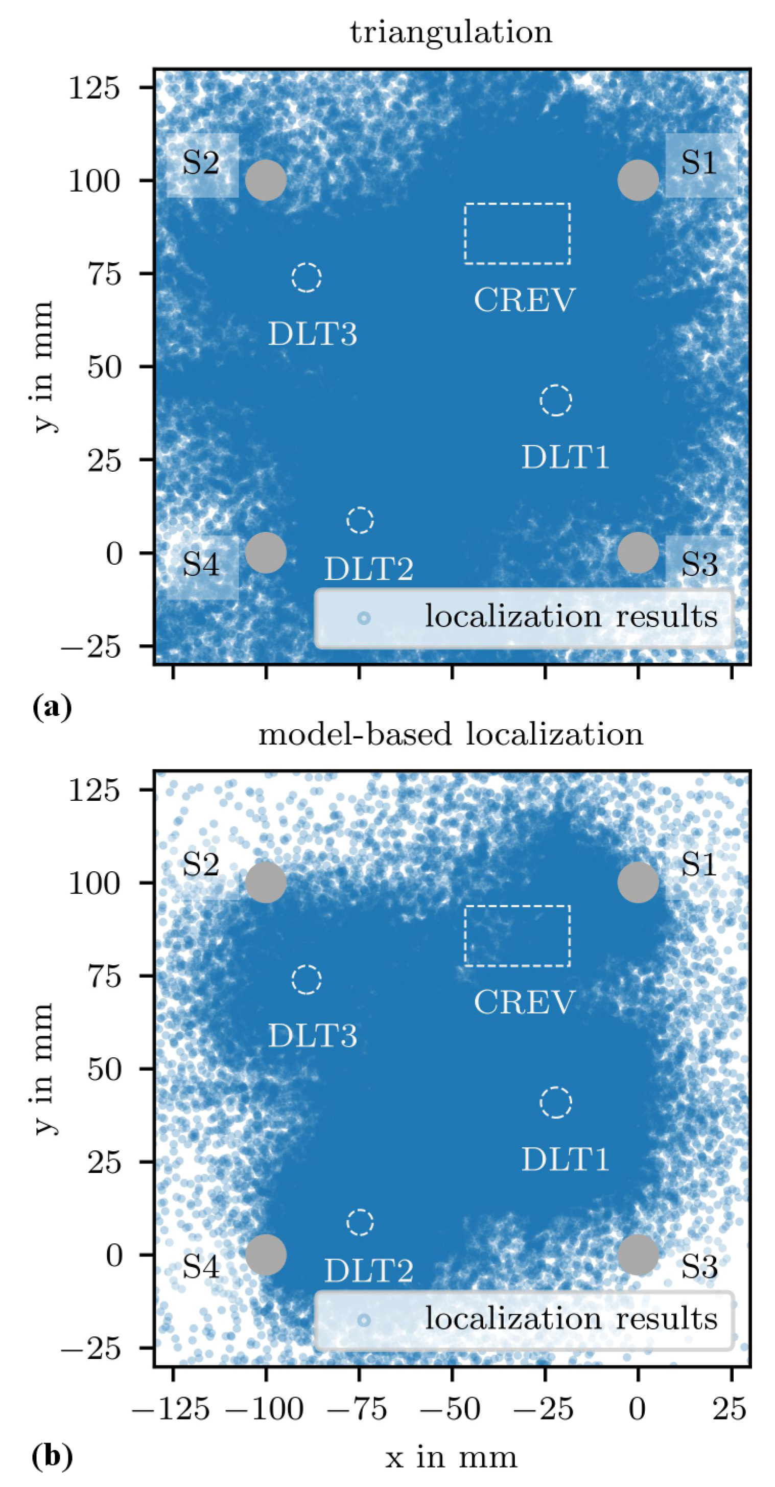
Figure 8.
Heat maps of localization results weighted by AE energy, referred to as AE-based corrosion images, (a) based on localization results obtained by triangulation using AIC TOA estimator, and (b) based on localization results obtained by model-based localization.
Figure 8.
Heat maps of localization results weighted by AE energy, referred to as AE-based corrosion images, (a) based on localization results obtained by triangulation using AIC TOA estimator, and (b) based on localization results obtained by model-based localization.
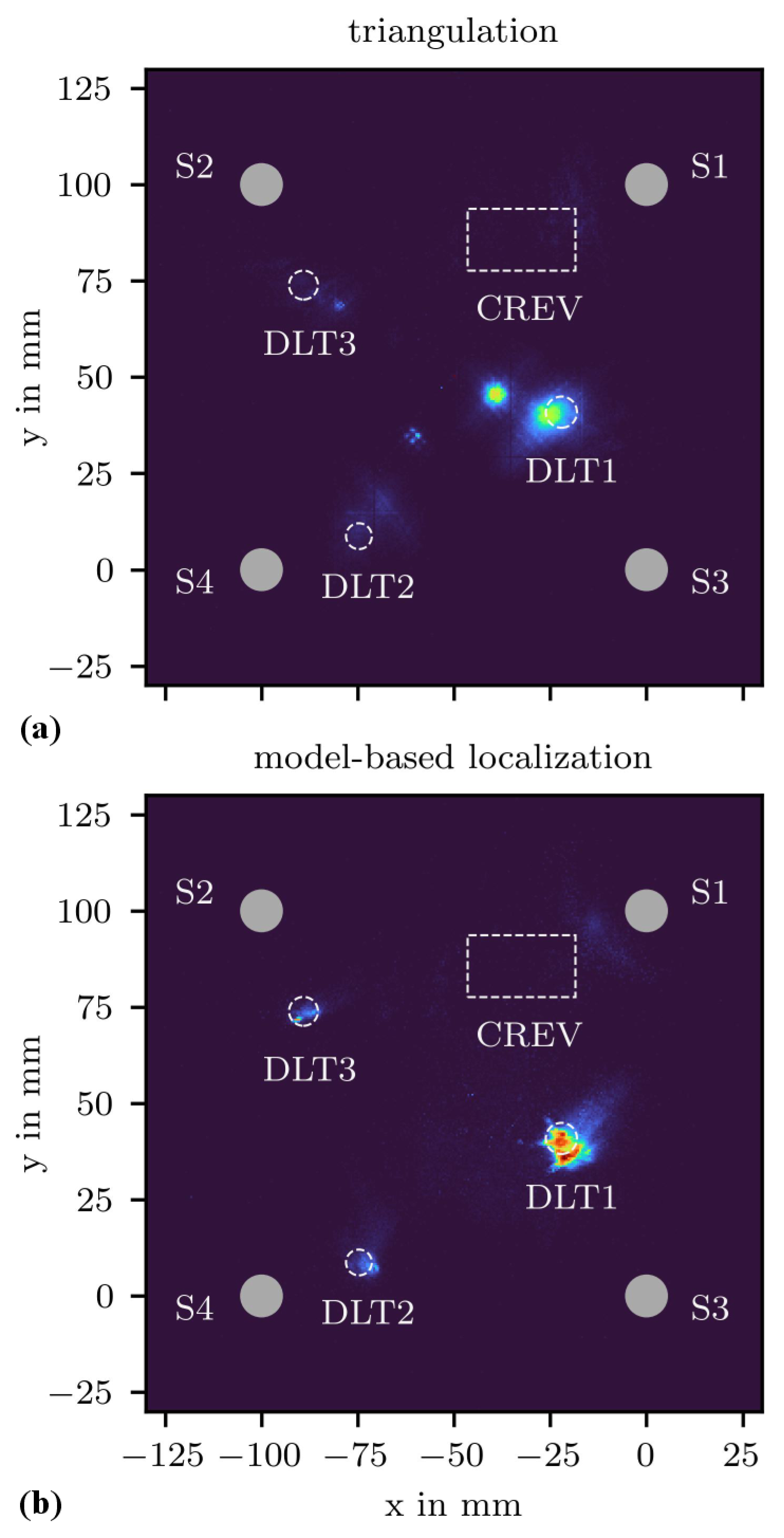
Figure 9.
Detail views of the AE based corrosion image, macroscopic photographs and the thresholded hue and brightness channel of corrosion sites (a) DLT1, (b) DLT2, (c) DLT3, and (d) CREV. The white dashed circles and rectangle in the corrosion images indicate the initially wetted surfaces. Spatially scattered AE activity corresponds to regions of uniform areal corrosion and accumulations of high AE activity to pitting corrosion or even specific pits.
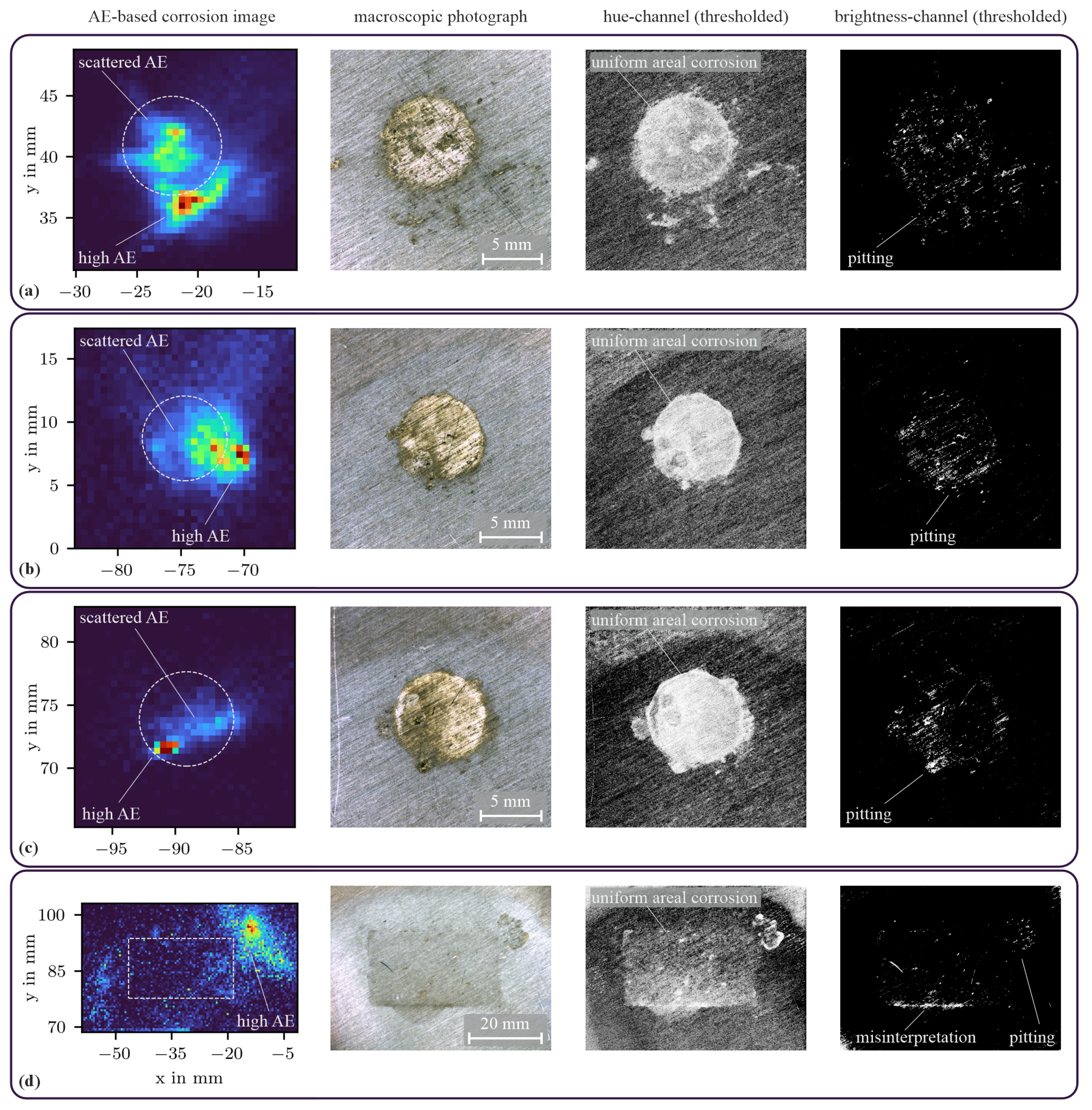
Figure 10.
Photograph of corrosion site DLT1 taken at the end of the experiment. The large amount of NaCl crystals, the repeated drying and re-wetting caused deliquescence over a larger area than the initially wetted area.
Figure 10.
Photograph of corrosion site DLT1 taken at the end of the experiment. The large amount of NaCl crystals, the repeated drying and re-wetting caused deliquescence over a larger area than the initially wetted area.
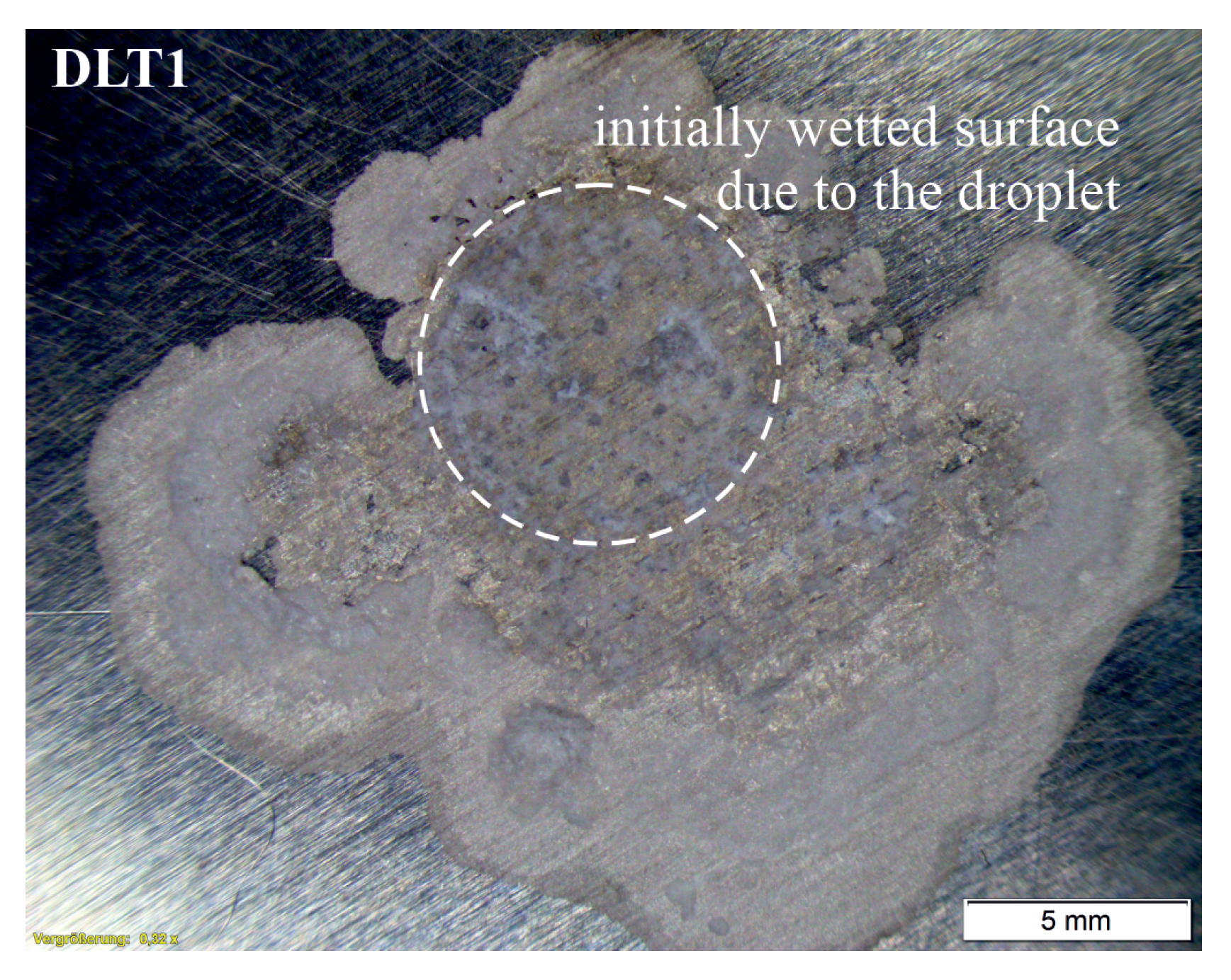
Figure 11.
Representative AE-based corrosion images of corrosion site DLT1, each considering AE activity within different 30-minute time windows during the experiment, as indicated above each image. (a-d) Representative corrosion images for phase ’wet@DLT1’, (e) representative corrosion image for phase ’re-wet@DLT1’, (f-j) representative corrosion images for phase ’re-wet@DLT1/2/3’, and (k-o) representative corrosion images for phase ’re-wet@DLT1/2/3+CREV’.
Disclaimer/Publisher’s Note: The statements, opinions and data contained in all publications are solely those of the individual author(s) and contributor(s) and not of MDPI and/or the editor(s). MDPI and/or the editor(s) disclaim responsibility for any injury to people or property resulting from any ideas, methods, instructions or products referred to in the content. |
© 2025 by the authors. Licensee MDPI, Basel, Switzerland. This article is an open access article distributed under the terms and conditions of the Creative Commons Attribution (CC BY) license (https://creativecommons.org/licenses/by/4.0/).
Copyright: This open access article is published under a Creative Commons CC BY 4.0 license, which permit the free download, distribution, and reuse, provided that the author and preprint are cited in any reuse.


