Submitted:
29 April 2025
Posted:
29 April 2025
You are already at the latest version
Abstract
Daily load following operation for a Molten Salt Reactor (MSR) was simulated by a DYMOS code. It simulates the reactor core by one-point kinetic equations considering the circulation and transit time of molten salt, also it simulates all plant components including a heat exchanger, a steam generator and a turbine/generator. The authors have verified the DYMOS code for transient results performed at the US experimental reactor MSRE, and results of accident analyses for a 700 MWt molten salt fast reactor based on a combined of detailed 3D thermal/hydraulic code and one-point point kinetic equations. In this paper, daily load-following operation of 100% to 50% (14-1-8-1 hour) for MSR-FUJI is simulated by the DYMOS code. It is shown that MSR-FUJI can be operated only by changing fuel salt flow rate without control rod motion. Also, since xenon poison effect is negligible in MSR-FUJI, the flow rate adjustment pattern is simple.
Keywords:
molten salt reactors
; load following operation
; reactivity control
; DYMOS code
1. Introduction
Molten Salt Reactor (MSR) is one of the 6 advanced reactors in the Generation-IV International Forum (GIF), and developmental efforts of MSR have been in progress in many countries [1,2,3]. The advantages of this concept are improved safety, proliferation resistance, resource sustainability, and waste reduction. MSR under consideration in this study uses high temperature molten fluorides salts as nuclear fuel and secondary cooling system. One of these developments is to evaluate plant system behaviors during normal operations and accidents, which is indispensable for MSR design and licensing. From this point of view, many analytical codes have been proposed [4,5]. Some studies have been reported on transient behavior for Molten Salt Fast Reactor (MSFR) [6,7]. They are built using mainly neutronics and thermal-hydraulics coupled computational fluid dynamics (CFD) code, e.g. COUPLE code [8], HEAT code [9], COMSOL code [10,11], OpenFOAM code [12,13,14,15]. In some cases, system code like TRACE [16] is used. Recently, the PROTEUS-NODAL code, which is a 3D nodal transport code, has been developed at Argonne National Laboratory and benchmarked with TRACE and CFD [17].
As discussed in the references [1,2,3], MSR has various advantages owing to liquid fuel concept. One of the advantages is that the MSR has excellent load-following capability, as discussed in an early study by Mitachi et al. [18]. However, previous analyses did not take into account a power generation system, and assumed instantaneous power changes, which do not accurately reflect actual daily load-following operation.
Recently, a transient analysis code DYMOS was developed by the authors, and validated by comparing its results with experimental data from the U.S. experimental reactor MSRE showing good agreement [19]. Besides that, comparison with results of accident analyses for a 700 MWt MSFR based on a combination of detailed 3D thermal/hydraulic code and one-point kinetic equations [20] showed good agreement [21]. Based on these validation results, the present study simulates daily load-following operation using the DYMOS code. As transients like daily load-following operation, reactor power and reactivity change quite slowly in comparison with accident transients, it is expected that the DYMOS code can evaluate load-following operation with the same accuracy as in the accident analyses.
The DYMOS code can evaluate system transient with enough accuracy in a very short computing time, for example, in a few seconds for a full day load-following calculation on an ordinary PC, when it is run without plotting the results at the same time. Such capability is quite useful for control system optimization, sensitivity study for various system parameters and so on. The objective of this study is to show applicability of the DYMOS code to analyses of daily load-following operation.
2. Description of the DYMOS Code [21] and the Reference Model [22]
A plant model, a reactor kinetics model, and a heat transfer model in the DYMOS code are described in Appendix A [21], in order to clarify the configuration of the plant and the simple lumped parameter model in the DYMOS code. Also, the model presented in the reference [22] is explained in Appendix B, in order to clarify the difference of our simple model and the detailed model in the reference study.
2.1. Remarks in the Proposed Study
There are two remarks in the DYMOS model for load-following simulations. The first one is that xenon (Xe-135) behavior is not considered in the model. In LWR daily load-following operation, Xe-135 affects reactivity and its compensation is required [23,24,25,26]. For example, in PWRs, control rods and boron concentration have to be adjusted all the period of daily load-following [25,26]. As for BWRs, core flow rate has to be always adjusted even within a narrow power change [23,24]. Meanwhile, in MSRs, gaseous fission products (FPs) such as xenon are continuously removed from the reactor core by the FP gas removal system [27]. Based on our evaluation, reactivity of Xe-135 in MSR-FUJI is 0.6 %Δk [28], and assuming 90% removal of Xe-135 efficiency, then its reactivity is only 0.06 %Δk, which can be neglected in the analyses. That is, Xe-135 behavior can be neglected in reactor operation during daily load-following cycles.
The second remark is as follows. In general, MSRs are designed to inject helium (He) bubbles in order to remove FP gas [27,29], and the amount of He injected is assumed to be approximately 0.5% of the fuel salt volume [30]. In the present analysis, it is assumed that the amount of He injected is proportional to the core flow rate. This design assumption is based on the consideration that, if the core flow rate is reduced while maintaining the same He injection rate, the volume of He within the core would increase and cause void reactivity change. The above assumption is intended to avoid such a complicated situation.
3. Verification of DYMOS Results for Daily Load Following Analysis
Since there are no preceding papers for MSR daily load-following operation, comparison was performed between the DYMOS code and a reference study for Molten Salt Breeder Reactor (MSBR) load-following in shorter time interval as 25 minutes [22]. This load-following operation is faster and shorter than daily load-following case (in 24 hours). As is described in Section 2.1, Xe-135 behavior is not necessary to be included, and then this faster operation is appropriate to verify the DYMOS code.
3.1. Comparison of DYMOS Results with a Detailed Model Study
Present study focuses on validation of the DYMOS code for applying to daily load-following operation. From this point of view, detailed model results for a linear load change transient, in which the load demand decreases from 100% Rated Power (RP) to 40% RP at a speed of 10% RP/min. after the steady-state operation for 100 sec., and then, the load demand returns to 100% RP at the same rate after equilibrium has been established at 40% RP [22]. Xenon transient is not included in the reference, because of the same reason explained in Section 2.1. In the reference study, it is not described clearly that the primary loop flow rate is constant (Primary loop flow rate controller is not shown in control diagrams.). In our study with the DYMOS code, the primary loop flow rate is assumed to keep constant.
The transient responses of the main system parameters are compared with DYMOS results in Figure 1, Figure 2, Figure 3 and Figure 4. The DYMOS code simulates the transient of this operation simply as follows. The main objective of the comparison here is to evaluate transient behavior of the DYMOS code for the primary loop, the simulation was performed and the results are shown as follows. That is, the secondary loop is not concerned here, because the parameters are control system dependent
Figure 1 shows reactor power and load demand as required (% of rated value). This is accomplished as the reference results are obtained with full control systems, the reactor power is controlled to follow the load demand.
Figure 2 shows control rod reactivity used to achieve required reactor power. The reason of small discrepancy seen in Figure 2 (also Figure 3 and Figure 4) would be due to the time delay of control system and the transport delay in the secondary loop.
Figure 3 and Figure 4 show transients of reactor inlet and outlet temperatures (Tin and Tout), respectively. These figures show that the results by the DYMOS code are in good agreement with those of the reference study.
As can be seen from the above description, the DYMOS model is a much simpler lumped parameter model than that presented in the reference. Even so, DYMOS analyses show similar results for daily load-following operations as explained above. As the conclusion of this section, the DYMOS code based on a lumped parameter model can be used for load-following operation for actual power plant.
4. Application of the DYMOS Code for Daily Load-Following Operation in MSR FUJI
As is described in Section 3, the DYMOS code is verified by the detailed model. Then, the DYMOS code is applied to daily load-following operation for MSR-FUJI. Plant description of MSR-FUJI and evaluation results are shown in this section.
4.1. Plant Description of MSR-FUJI
MSR-FUJI is designed as a graphite moderated thermal MSR. The power output is reduced to 350 MWt, but all of the characteristics are similar to that of the referenced 2250 MWt MSBR [27]. In this study, the reactor core under consideration is FUJI-12 [31]. Main design parameters are listed in Table 1
4.2. Evaluation of Daily Load-Following Operation Without Control Rod
In this study, a representative example of daily load-following operation, known as the “14-1-8-1” mode, was considered. That is, the reactor operates at 100% output for 14 hours during the daytime, reduces output to 50% for 8 hours at night, and transitions linearly between these states in a 1-hour period. To achieve this operational mode, the DYMOS code was used to maintain reactor criticality while adjusting the fuel salt flow rate accordingly. The generator output was also assumed to follow the same pattern.
Figure 5 shows power and flow rate. It is shown that flow rate is kept higher than the relative power to adjust reactivity. Figure 6 shows the temperature transitions at various points in the system, including the core inlet and outlet, graphite, heat exchanger, and steam generator.
The results indicate that the core outlet temperature remains nearly constant even during the low-power operation at night, while the inlet temperature exhibits a slight increase. These results show that MSR can operate daily load-following only by changing flow rate, and does not need to use control rod movement. Furthermore, as is described in Section 2.1, since reactivity change due to Xe-135 is negligible in MSR-FUJI, flow rate at day-time or night-time is maintained almost constant.
5. Conclusion
The DYMOS code is a very simple lumped parameter model, however, it can evaluate daily load-following operations with similar accuracy obtained by much detailed distributed parameter models. The reason that such a simple model can evaluate reactor transient is due to the simplicity of the reactor design. In other words, the reactor can be treated as a homogeneous system and fuel has no burnup distribution within the reactor core, thus the reactor can be treated as a simple homogeneous heat source. Reactivity coefficients are negative, which can support stable reactor operation.
From the above results, it was demonstrated that daily load-following operation with a large variation between 100% and 50% power can be achieved only by adjusting the fuel salt flow rate, without control rod operation. Furthermore, since FP gas such as xenon is always removed in MSRs, Xe-135 reactivity change is negligible in load following operation. Owing to this advantage, the required flow rate pattern is very simple during load-following operation.
Author Contributions
Conceptualization, Ritsuo Yoshioka.; methodology, Yoichiro Shimazu.; software, validation, Yoichiro Shimazu.; investigation, Ritsuo Yoshioka.; resources, Ritsuo Yoshioka.; data curation, Ritsuo Yoshioka.; writing—original draft preparation, Yoichiro Shimazu.; writing—review and editing, Yoichiro Shimaz., Ritsuo Yoshioka. All authors have read and agreed to the published version of the manuscript.
Funding
This research received no external funding.
Data Availability Statement
We encourage all authors of articles published in MDPI journals to share their research data. In this section, please provide details regarding where data supporting reported results can be found, including links to publicly archived datasets analyzed or generated during the study. Where no new data were created, or where data is unavailable due to privacy or ethical restrictions, a statement is still required. Suggested Data Availability Statements are available in section “MDPI Research Data Policies” at https://www.mdpi.com/ethics.
Conflicts of Interest
The authors declare no conflicts of interest.
Appendix A. Description pf the DYMOS code [21]
Appendix A.1. Plant Model in the DYMOS Code
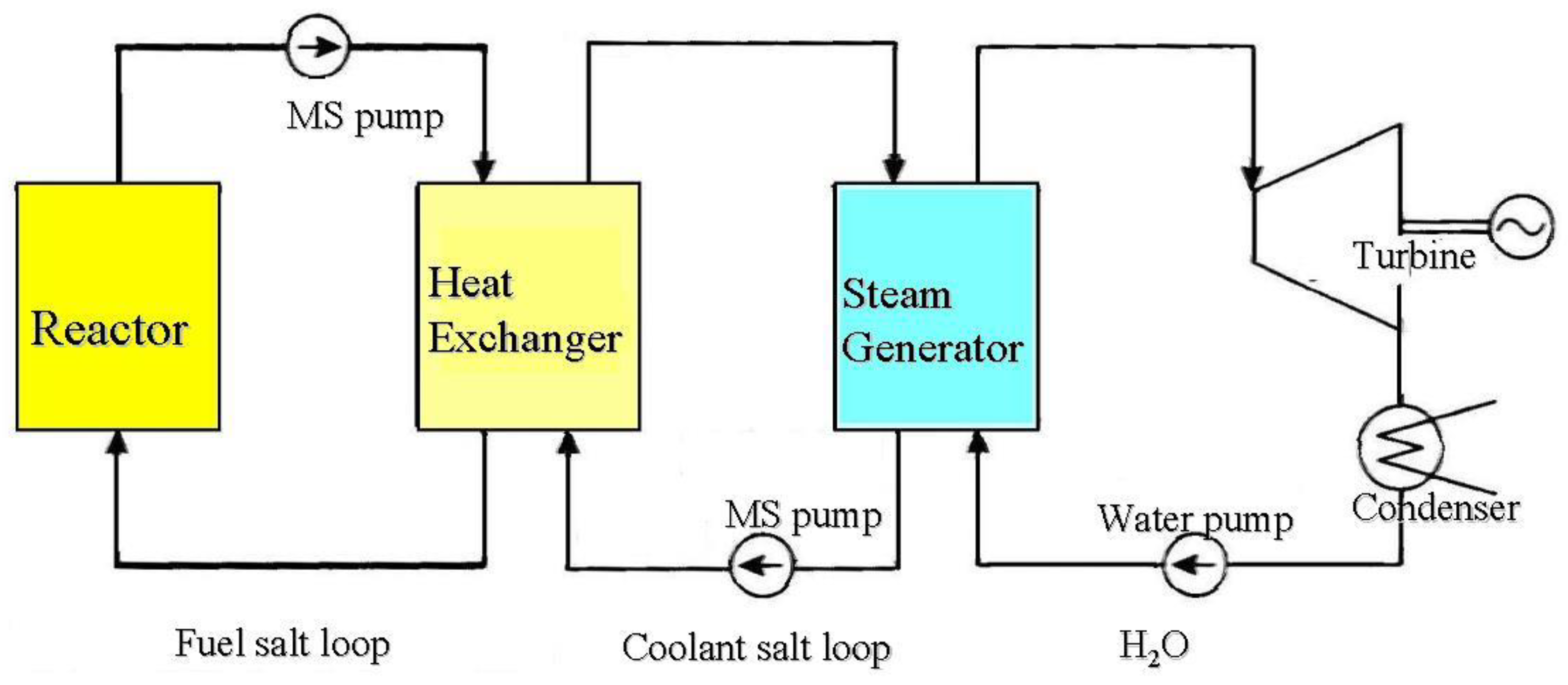
Figure A1 illustrates a simplified plant configuration as represented in the DYMOS code. The operational concept of Molten Salt Reactors (MSRs) significantly differs from that of conventional reactors such as light water reactors (LWRs), which typically employ solid-type nuclear fuel. Meanwhile, MSR adopts liquid-type nuclear fuel such as molten salt. As outlined in references [1,2,3], MSRs offer several key advantages, including enhanced safety features, reduced risk of nuclear proliferation, improved sustainability of fuel resources, and decreased production of radioactive waste.
The MSR examined in this study utilizes high-temperature molten fluoride salt, which serves as the nuclear fuel in a primary loop, and serves as the medium for heat transfer in a primary loop and a secondary loop. The fuel salt contains fissile and fertile materials as fluoride. Within the reactor, the circulating fuel salt sustains criticality, and undergoes fission reactions to produce thermal energy. This nuclear heat is carried from the reactor core to a primary heat exchanger (HX) via the primary fuel salt loop. From there, thermal energy is conveyed to a steam generator (SG) through the secondary coolant salt loop, and ultimately converted to mechanical energy in a turbine-generator, provided the plant operates with a steam turbine system.
Due to the circulation of the fuel salt in the primary loop, a portion of delayed neutron precursors exits within the reactor core, with some eventually returning. This dynamic behavior is a distinctive aspect of MSR neutron kinetics. Beyond the point where heat is transferred to the secondary loop, however, the system operates similarly to a conventional thermal energy transport system.
Based on the above considerations, each component and loops such as the fuel salt loop (primary loop) and subsequent loops of the DYMOS code are shown in Figure A1.
Appendix A.2. Reactor Kinetics Model
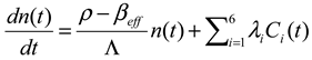
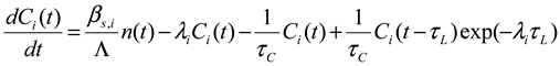
The DYMOS code employs one-point kinetic equations to model reactor power, as outlined below. These equations are almost consistent with those traditionally used in the licensing analysis of LWRs. In fact, Equations (A1) and (A2) closely resemble the standard one-point kinetic equations found in classical reactor physics literature [3]. What sets the MSR model apart is the explicit consideration of delayed neutron precursor behavior within the circulating fuel salt. This is reflected in the third and fourth terms of the second equation, originally introduced by ORNL [32]. In other words, the conventional kinetics model, which has been developed for reactors using solid fuel, was modified to account for both the loss of precursors that exit the core with the flowing salt and the gain as some precursors return. To facilitate simplification of Equation (A1), two new parameters have been introduced: βeff and βloss. These definitions are intended to streamline the mathematical treatment while preserving the physical meaning of precursor dynamics in flowing fuel systems. These equations are solved, assuming the reactor is operated at constant before time-zero.
: Number of neutrons
: Number of delayed neutron precursor of i-th group
: Decay constant of i-th group delayed neutron precursor
: Effective delayed neutron fraction
: Delayed neutron fraction for static reactor of its group
βloss: Loss fraction of delayed neutron by fuel salt flow
: Neutron generation time
τC: Fuel transit time in the reactor core
τL: Fuel transit time in the primary loop outside the reactor core
: Reactivity
; Fuel temperature and its rated value
; Graphite temperature and its rated value
; Fuel temperature reactivity coefficient
; Graphite temperature reactivity coefficient
; External reactivity
Appendix A.3. Heat Transfer Model
The thermal energy produced by nuclear fission is first carried to a (primary) heat exchanger via the circulating fuel salt loop. From there, it is transferred to a steam generator (SG), and ultimately to the power generation system. The corresponding temperatures throughout these stages can be determined by analyzing the energy balance across the system. The current plant model adopts a simplified, lumped-parameter approach, representing each subsystem as a single point. The governing equations used to describe this model are provided below. These expressions are either directly adapted from, or further simplified versions of, the models discussed in reference [32].
: Fuel salt temperature at reactor outlet, reactor inlet, heat exchanger, and steam generator
: Fuel mass
: Specific heat of fuel salt
: heat transfer area and heat transfer coefficient in respective system
: Fuel flow mass rate
: Thermal power output (=fission power + decay heat)
: Heat generation in graphite moderator
: Heat sink in the steam generator
Here, the term C(t-) in Equation (A2) accounts for the transit time, associated with the circulation of molten salt within the loop. Various modeling approaches have been proposed to describe salt transport through piping. In this study, the simplest approach, which is a first-order time-lag model with a delay time of , is adopted, following the methodology outlined in the reference [33]. The transfer function of this treatment is shown below.
This model is also applied to the temperature of returning fuel salt in the above Equation (A6).
The set of differential Equations (A1) through (A10) is solved using numerical integration. A time step of 0.1 seconds is employed. Since a shorter time step of 0.01 seconds provided identical results, the above 0.1 seconds was confirmed to be sufficiently small for accurately calculating the dynamics involved in daily load-following operations. The simplicity of the nuclear and thermal models contributes to their transparency, that is, the models are readily comprehensible to safety experts and can be easily replicated for regulatory or licensing assessments.
Appendix B. Description of the Model in the Referenced Study [22]
Appendix B.1. Description of the Reference Model
Description of the reference model is re-listed briefly here. It explains how well the plant is modeled in detail, compared with the DYMOS code.
The objective of the referenced study is to develop a comprehensive simulation platform capable of evaluating the control characteristics of a MSR plant under both normal and accident conditions. For this purpose, the 2250 MWt MSBR concept [27] was adopted as the reference design for system modeling and controller development. The simulation platform incorporates a nonlinear distributed-parameter model of the entire system, which includes a liquid-fueled reactor core with a graphite moderator, an intermediate heat exchanger, and a steam generator. Meanwhile, the DYMOS code adopts a lumped parameter model, which is simple but is verified having enough accuracy [21].
A novel control strategy is introduced, integrating both feedforward and feedback control schemes. This strategy is designed to respond to load variations by coordinating reactor power and steam temperature control systems, while accounting for input saturation and dead zones. Meanwhile, the DYMOS code does not include the delay by the control systems. This difference might affect the results of load-following simulations, as is shown in Section 3.
To accurately capture the temperature distributions within the system, the reactor core is discretized into N axial nodes and two radial zones for both the liquid fuel and the graphite moderator. Similarly, the molten fuel salt, heat exchanger tube walls, and secondary coolant salt are divided into N axial nodes. The steam generator is discretized in a comparable manner to ensure consistency in the thermal-hydraulic modeling. Meanwhile, the DYMOS code adopts one-point model for the reactor core. For example, since the reactor core of MSR is simple, that is only molten fuel salt and graphite exist in MSR-FUJI, the influence of temperature distribution is very small for transient behavior, as is verified in the previous study [21].
Table A1 shows main design parameters of the reference plant, and Table A2 shows parameters of heat transfer systems.

Table A1.
Main design parameters [22].
Table A1.
Main design parameters [22].
| Parameters | Values |
|---|---|
| Total thermal power (MW) | 2250 |
| Core height (m) | 3.96 |
| Central zone/Outer zone diameters (m) | 4.39/5.15 |
| Total delayed neutron fraction (pcm) | 264 |
| Core transit time of fuel salt τc (s) | 3.57 |
| External loop transit time of fuel salt τL (s) | 6.05 |
| Reactivity coefficient of fuel (1/K) | −2.4 × 10⁻⁵ |
| Reactivity coefficient of graphite (1/K) | 1.9 × 10⁻⁵ |
| Primary fuel salt | LiF-BeF2-ThF4-UF4 |
| Core inlet temperature (K) | 838.7 |
| Core outlet temperature (K) | 977.6 |
| Fuel salt flow rate (kg/s) | 11945 |
| Secondary salt | NaBF4-NaF |
| Secondary salt cold-leg temperature (K) | 727.6 |
| Secondary salt hot-leg temperature (K) | 894.3 |
| Secondary salt flow rate (kg/s) | 8971 |
| Feed water inlet temperature (K) | 644.3 |
| Steam outlet temperature (K) | 810.9 |
| Steam flow rate (kg/s) | 1487 |
| Steam pressure (MPa) | 24.82 |
Table A2.
Parameters of heat transfer systems [22].
Table A2.
Parameters of heat transfer systems [22].
| Parameters | Values |
|---|---|
| Fuel salt specific heat (J·kg−1·K−1) | 1357 |
| Graphite density (kg·m−3) | 1843 |
| Graphite specific heat (J·kg−1·K−1) | 1760 |
| Fuel-graphite heat transfer coefficient (W·m−2·K−1) | 6047 |
| Secondary salt density (kg·m−3) | 2252 − 0.711(T − 273) |
| Secondary salt specific heat (J·kg−1·K−1) | 1507 |
| Tube wall density (kg·m−3) | 8671 |
| Tube wall specific heat (J·kg−1·K−1) | 569 |
| IHX fuel salt-wall heat transfer coefficient (W·m−2·K−1) | 13,786 |
| IHX secondary salt-wall heat transfer coefficient (W·m−2 ·K−1) | 9533 |
| Supercritical water/steam density (kg·m−3) | 2.144 × 10⁻²T2 − 33T + 12,748 |
| Supercritical water/steam specific heat (J·kg−1·K−1) | 1.797T2 − 2802T + 1.095 × 10⁶ |
| SG secondary salt-wall heat transfer coefficient (W·m−2·K−1) | 4860 |
| SG water inlet-wall heat transfer coefficient (W·m−2·K−1) | 10,055 |
| SG steam outlet-wall heat transfer coefficient ( W·m−2·K−1) | 8265 |
Appendix B.2. Molten Salt Reactor
The neutron kinetics of the reactor are modeled using one-point kinetic equations, incorporating the drift of delayed neutron precursors as well as temperature reactivity feedbacks from both the molten fuel salt and the graphite moderator, as described in the previous section. That is, the reactor kinetics model is identical to the DYMOS code.
Appendix B.3. Heat Exchanger
The heat exchanger (HX) is designed as a shell-and-tube type, in which the primary fuel salt flows downward through the tube side, while the secondary salt flows upward through the shell side, which is divided to N axial nodes. Meanwhile, the DYMOS code regards the HX as a simple lumped parameter (one-point) model. But, as far as heat transfer in the loop, this simple model can be used.
Appendix B.4. Steam Generator
The steam generator (SG) adopts a U-tube counter-current flow configuration, which is divided to N axial nodes. High-temperature secondary salt enters the shell side, while feedwater is introduced into the U-tube side, where it is converted into superheated steam via heat exchange with the secondary salt. The SG system is modeled in detail to accurately capture its thermal behavior. Meanwhile, the DYMOS code regards the SG as a simple lumped parameter (one-point) model. But, as far as heat transfer in the loop, this simple model can be used.
Appendix B.5. Transport Time Delay Between Various Systems
To account for the transport time of fluid between subsystems, transport delay equations are incorporated into the dynamic simulation platform. For the primary loop, the delays between the reactor core and the HX are modeled same as MSBR plant:
where Tp,in and Tp,out are the corresponding temperatures in the HX. And, Tf,in and Tf,out represent the inlet and outlet temperatures of the primary fuel salt in the reactor core. The delay times are τd1=2.0 sec. and τd2=2.3 sec.
For the secondary loop, transport delays in the hot and cold legs are similarly defined as:
where Tss and Ts are the secondary-salt temperatures in the heat exchanger and the steam generator, respectively, the values of delay times and are 14.5 sec. and 11.9 sec. [33]. Meanwhile, the DYMOS code does not take into account of these time delay except the equation (A12), because the time delay is compensated by the controller and thus the effect of the simplification on the primary system is negligible. Also, in this study, since primary system behavior is mainly focussed, this simple model can be used.
Appendix B.6. Reactor Power Control System
In response to variations in the electric grid load, the desired reactor power output is determined and translated into a corresponding set-point for the neutron flux. The deviation between this set-point and the measured neutron flux is input to a PID (Proportional Integral Derivative) controller. The resulting control signal is processed to generate an adjustment command, which is then sent to the control rod drive mechanism to determine the appropriate speed and direction of rod movement. Additionally, the feedwater control system and the steam generator control system are integrated into the overall control strategy to ensure coordinated plant operation. Also, the feed water controller and steam generator control system are taken into account. As is discussed in B.1, the DYMOS code does not include the delay by the control systems. This difference might affect the results of load-following simulations, as is shown in Section 3.
References
- Serp, J.; et al. The Molten Salt Reactor (MSR) in Generation IV: Overview and Perspectives. Progress in Nuclear Energy 2014, 77, 308–319. [Google Scholar] [CrossRef]
- IAEA. Status of Molten Salt Reactor Technology. TRS-489. 2023. [Google Scholar]
- Dolan, T.J. (Ed.) Molten Salt Reactors and Thorium Energy; Woodhead Publishing (Elsevier), 2017 & 2024. [Google Scholar]
- Krepel, J. Dynamics of Molten Salt Reactors. Ph.D. Thesis, PSI, 2006. [Google Scholar]
- Wooten, D.; Powers, J.J. A Review of Molten Salt Reactor Kinetics Models. Nucl. Sci. Eng. 2018, 191, 203–230. [Google Scholar] [CrossRef]
- Brovchenko, M.; Heuer, D.; Merle-Lucotte, E.; et al. Design-related studies for the preliminary safety assessment of the molten salt fast reactor. Nucl Sci Eng. 2013, 175, 329–339. [Google Scholar] [CrossRef]
- Brovchenko, M.; Merle-Lucotte, E.; Heuer, D.; et al. Molten salt fast reactor transient analyses with the COUPLE code, Proc. of the ANS Annual Meeting, Atlanta, USA. 2013. Available online: https://www.researchgate.net/publication/275019982.
- Zhang, D.; Zhai, Z.-G.; Rineiski, A.; et al. COUPLE. A time-dependent coupled neutronics and thermal- hydraulics code, and its application to MSFR, Proc. of the 2014 22nd International Conference on Nuclear Engineering (ICONE22), Prague, Czech, ICONE22–30609. 2014. [Google Scholar] [CrossRef]
- Fiolina, C. The molten salt fast reactor as a fast- spectrum candidate for thorium implementation. Ph.D. Thesis, Politechnico di Milano, 2013. [Google Scholar]
- Comsol Multiphysics®. COMSOL Multiphysics programming reference manual. 2018. Available online: https://doc.comsol.com/5.4/doc/com.comsol.help.comsol/COMSOL_ProgrammingReferenceManual.pdf.
- Laureau, A.; Heuer, D.; Merle-Lucotte, E.; et al. Transient coupled calculations of the molten salt reactor using the transient fission matrix approach. Nucl Eng Des. 2017, 316, 112–124. [Google Scholar] [CrossRef]
- Gérardin, D. Développement de méthodes et d’outils numériques pour l’étude de la sûreté du réacteur à sels fondus MSFR. Ph.D. Thesis, Grenoble Institute of Technolog, 2019. Available online: https://tel.archives-ouvertes.fr/tel-01971983/document.
- Wan, C.; Hu, T.; Cao, L. Multi-physics numerical analysis of the fuel-addition transients in the liquid-fuel molten salt reactor. Ann Nucl Energy 2020, 144, 107514. [Google Scholar] [CrossRef]
- Gonzalez Gonzaga de Oliveira, R. Improved methodology for analysis and design of molten salt reactors, PhD thesis, École Polytechnique fédérale de Lausanne, Thèse No 8618. 2021. [Google Scholar]
- OpenFOAM®. OpenCFD Release OpenFOAM® 1912. 2019. Available online: https://www.openfoam.com/news/main-news/openfoam-v1912.
- Pettersen, E.E. Coupled multi-physics simulations of the molten salt fast reactor using coarse- mesh thermal-hydraulics and spatial neutronics. Master’s Thesis, Paris-Saclay University, 2016. Available online: https://www.psi.ch/sites/default/files/import/fast/PublicationsEN/FB-DOC-16-016.pdf.
- Jaradat, M.K.; Park, H.; Yang, W.S.; et al. Development and validation of PROTEUS-NODAL transient analyses capabilities for molten salt reactors. Ann Nucl Energy 2021, 160, 108402. [Google Scholar] [CrossRef]
- Yamamoto, T.; Mitachi, K.; Nishio, M. Characteristics of 3-Core Molten Salt Reactor Study on Load-following Capability. The Heat Transfer Society of Japan, Proceedings 2007, 15. (In Japanese) [Google Scholar]
- Yoshioka, R.; Shimazu, Y.; Ogasawara, K.; Furukawa, M. Transient Analysis Code for Molten Salt Reactor: DYMOS (in Japanese), Proceedings of AESJ Autumn conference. 2021. [Google Scholar]
- Mochizuki, H. Neutronics and Thermal-hydraulics Coupling analyses on transient and accident behaviors of molten chloride salt fast reactor. Journal of Nuclear Science and Technology 2018. [Google Scholar] [CrossRef]
- Shimazu, Y.; Yoshioka, R.; Ogasawara, K. Proposal of Application of a Simple Analysis Code DYMOS for Accident Analyses of Molten Salt Reactors. Journal of Energy Research and Reviews 2023, 15, 18–33, Article no. JENRR.110642, ISSN: 2581-8368. [Google Scholar] [CrossRef]
- Luo, R.; Liu, C.; Macián-Juan, R. Investigation of Control Characteristics for a Molten Salt Reactor Plant under Normal and Accident Conditions. Energies 2021, 14, 5279. [Google Scholar] [CrossRef]
- Maruyama, H.; et al. Core Design and Operating Strategies for Better Daily Load Following Performance in BWR Cores. Journal of Nuclear Science and Technology 1984, 21, 550–557. [Google Scholar] [CrossRef]
- Tanabe, A.; et al. Daily Load Following Operation of BWR Power Plant (in Japanese). Toshiba Review 1979, 34, 832–836. [Google Scholar]
- Calic, D.; et al. Simulation of Load Following Operation with a PWR reactor. Proceedings of the International Conference Nuclear Energy for New Europe, Portoroz, Slovenia. 2022. [Google Scholar]
- Muniglia, M.; et al. Design of a Load Following Management for a PWR Reactor Using an Optimization Method. International Conference on Mathematics & Computational Methods Applied to Nuclear Science & Engineering. 2017. [Google Scholar]
- Robertson, R.C. Conceptual Design Study of a Single-fluid Molten-Salt Breeder Reactor, ORNL-4541. 1971. [Google Scholar]
- Suzuki, K. Shimazu, Evaluation of Xenon Effect for Small Molten Salt Reactor FUJI12, Private communication. 2012. [Google Scholar]
- Gabbard, C.H. Development of a Venturi Type Bubble Generator for Use in the Molten-Salt Reactor Xenon Removal System. ORNL-TM-4122. 1972. [Google Scholar]
- Suzuki, N.; Shimazu, Y. Preliminary Safety Analysis on Depressurization Accident without Scram of a Molten Salt Reactor. Journal of Nuclear Science and Technology 2006, 43, 720–730. [Google Scholar] [CrossRef]
- Mitachi, K.; Okabayashi, D.; Suzuki, T.; Yoshioka, R. Re-estimation of Nuclear Characteristics of a Small Molten Salt Power Reactor (in Japanese). Journal of Atomic Energy Society in Japan 2000, 42, 9. [Google Scholar]
- Sides, W.H. MSBR Control Studies, ORNL-TM-3102. 1971. [Google Scholar]
- Sides, W. MSBR Control Studies: Analog Simulation Program; Technical Report, ORNL-TM-2927; Oak Ridge National Lab.: Oak Ridge, TN, USA, 1971. [Google Scholar]
Figure 1.
Power change pattern.
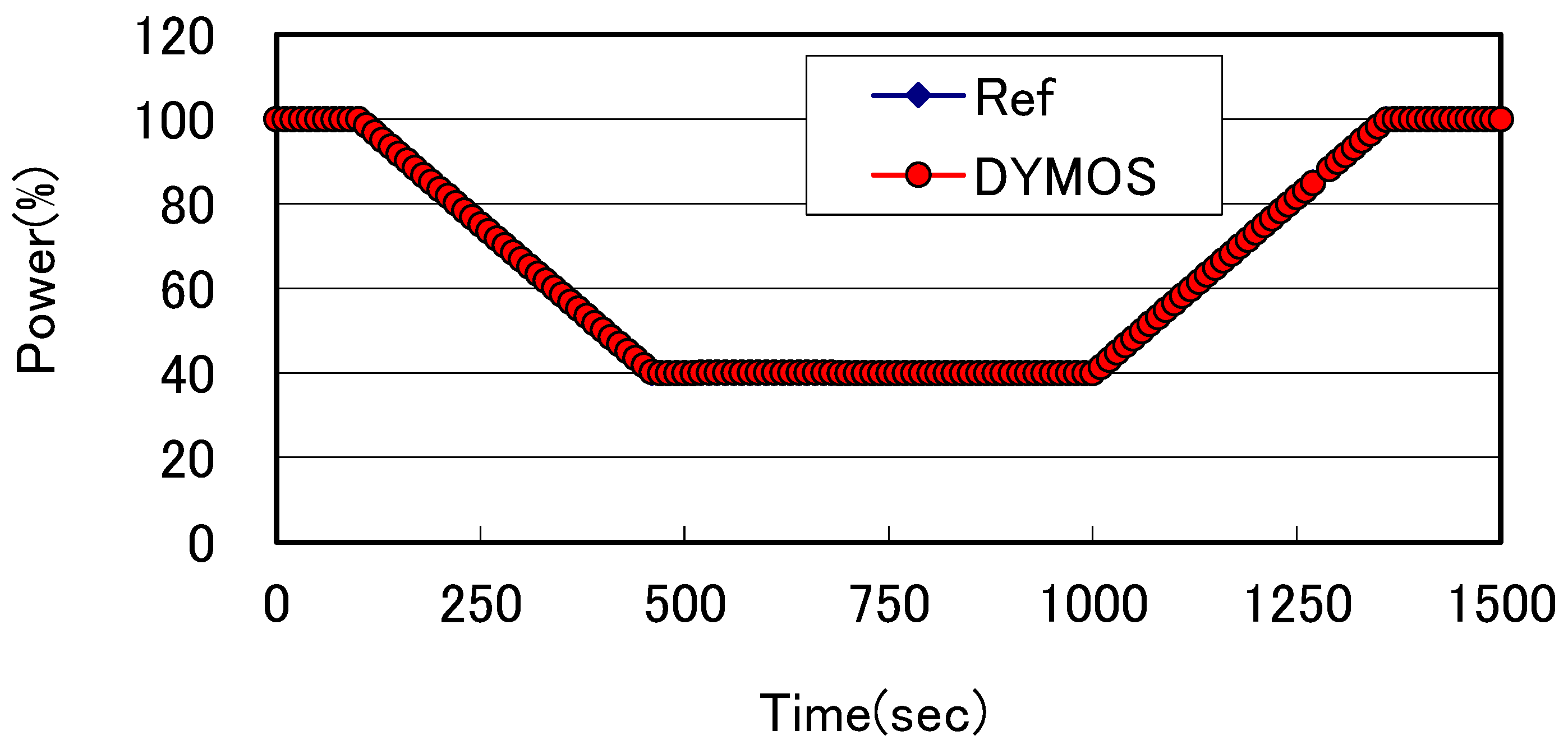
Figure 2.
Control rod reactivity.
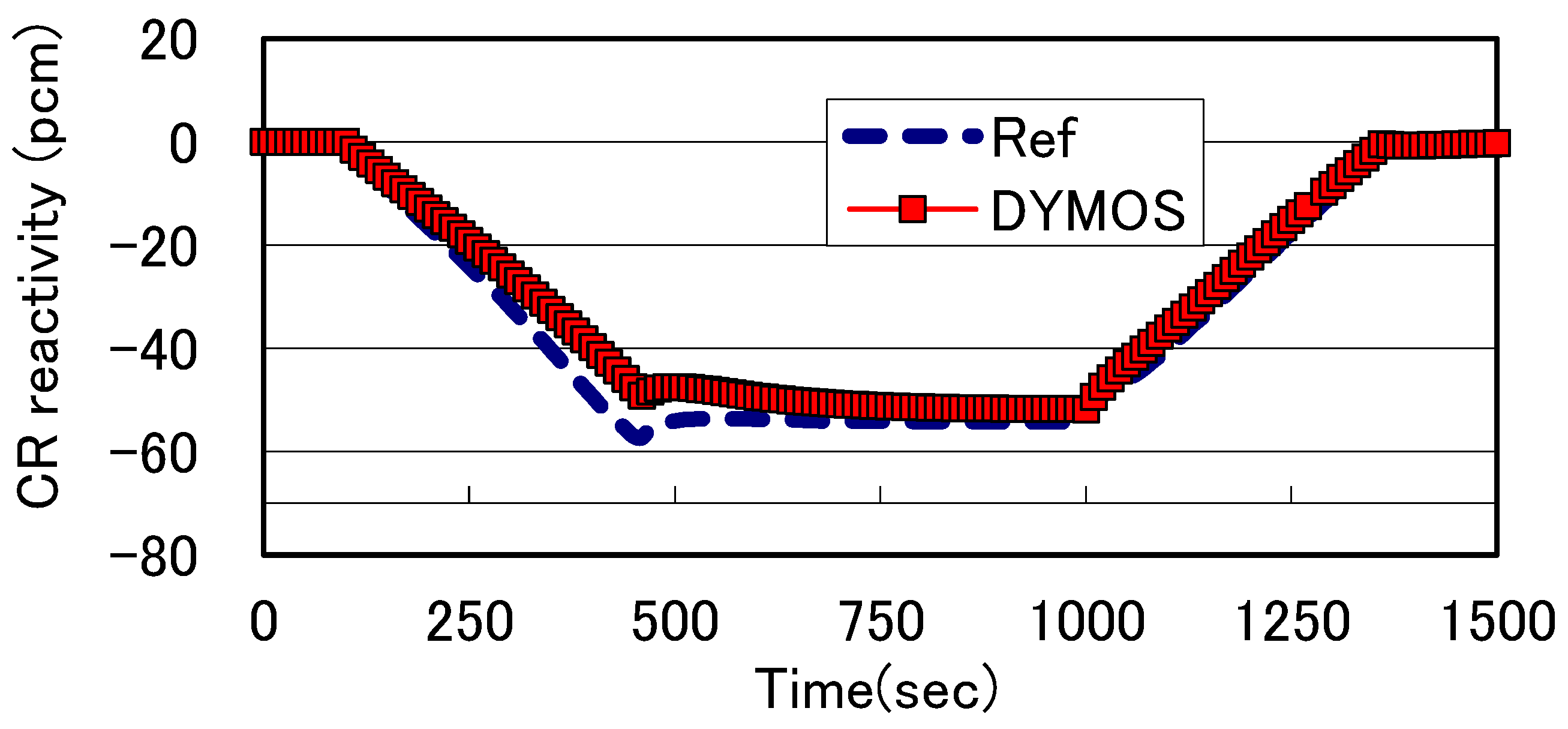
Figure 3.
Tin variation.
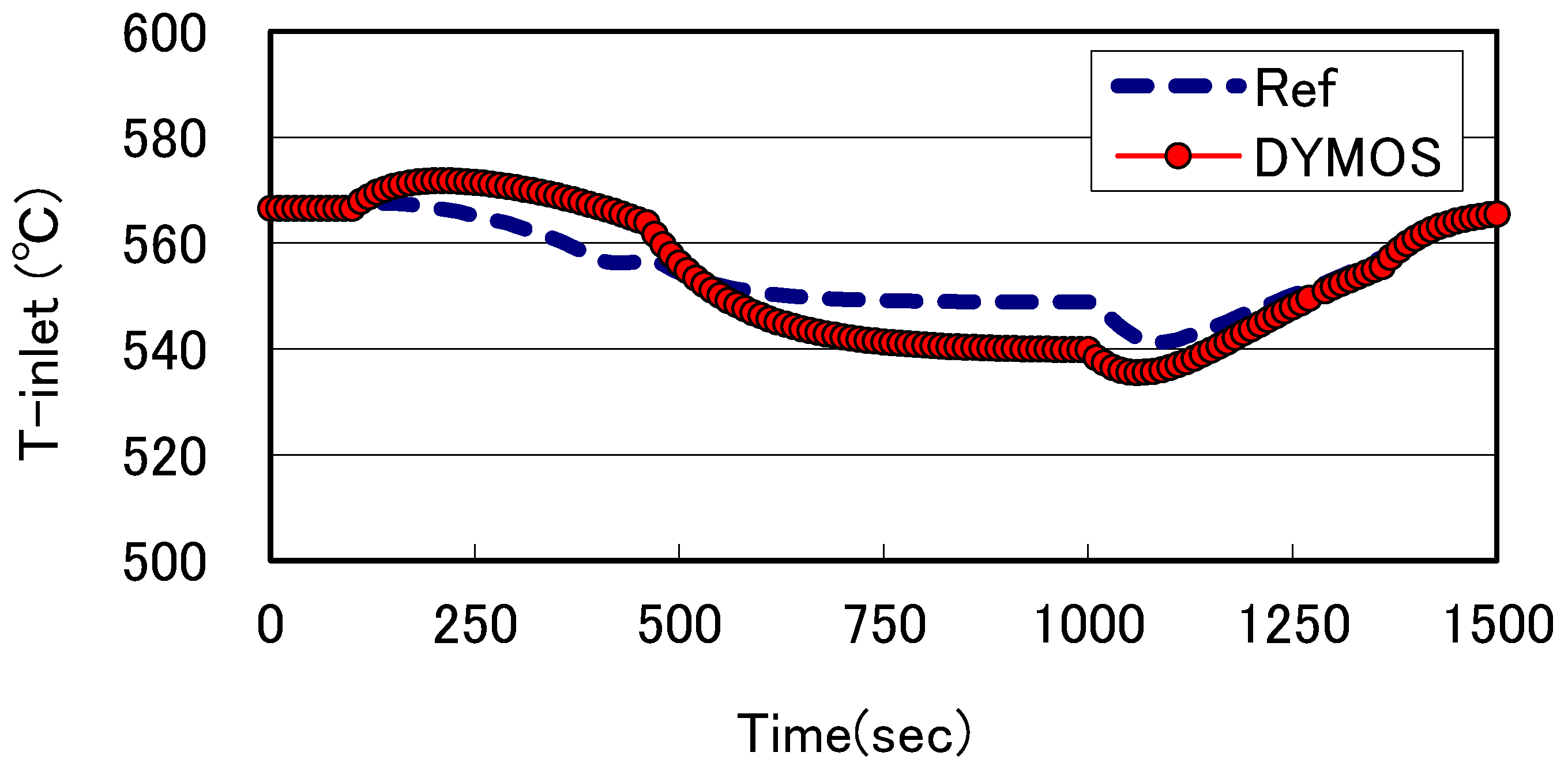
Figure 4.
Tout variation.
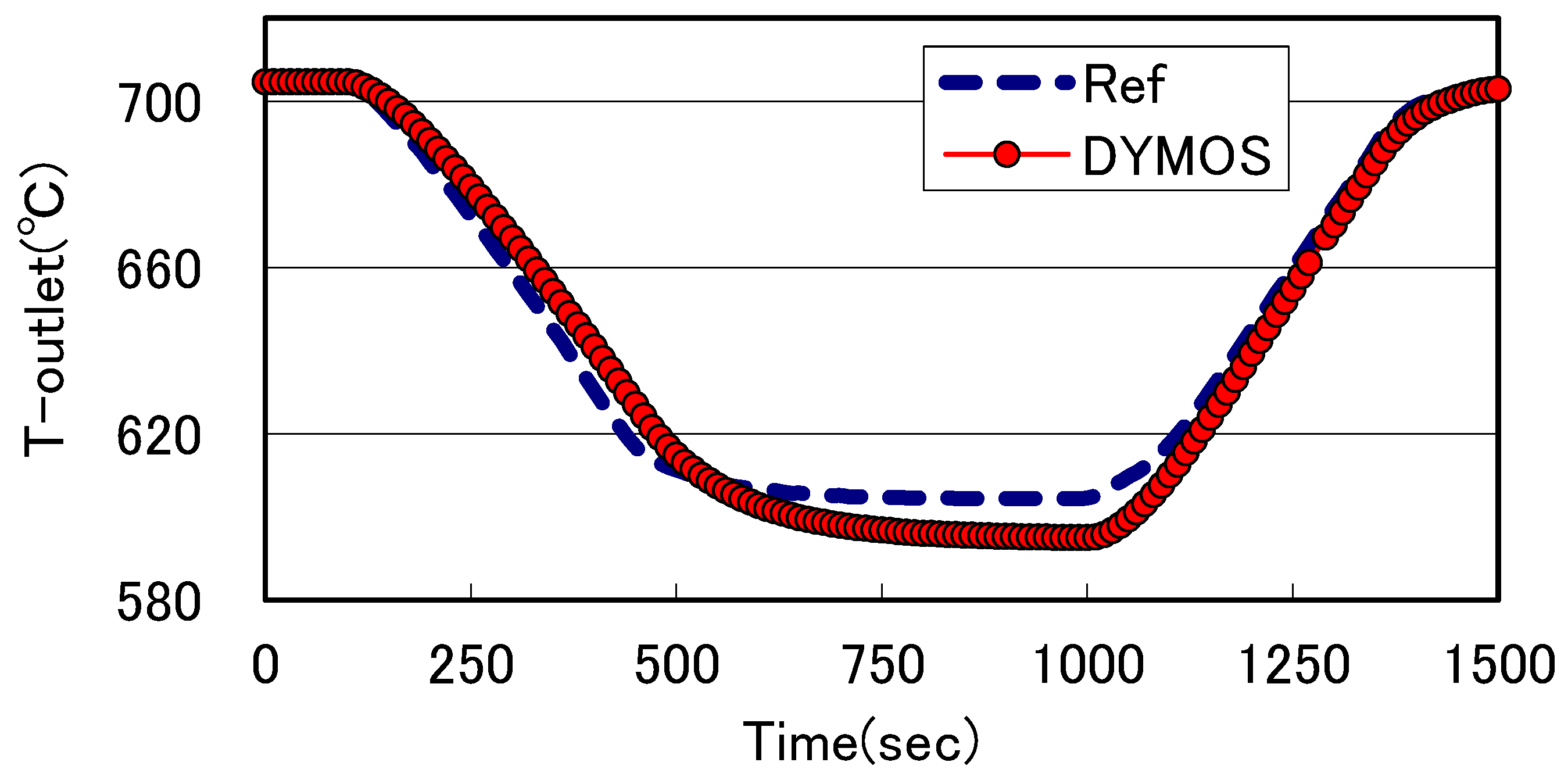
Figure 5.
Power and flow rate.
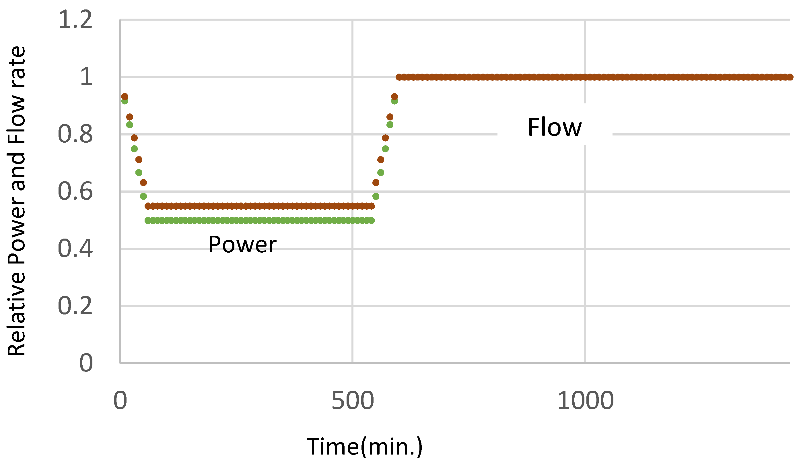
Figure 6.
System temperatures.
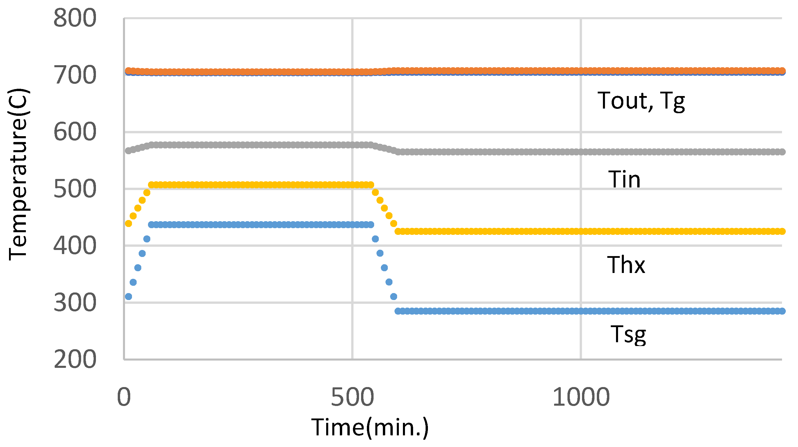
Table 1.
Main design parameters of FUJI-12 [31].
Table 1.
Main design parameters of FUJI-12 [31].
| Main Specifications of FUJI-12 |
|---|
|
Thermal power: 350 MWth Electric power output: 150 MWe Core radius/height: 2.0 m/4.0 m Graphite fraction in the core: 70 vol% Fuel salt temperature (Outlet/Inlet): 980 K/840 K Fuel salt composition: LiF (71.78 mol%), BeF2 (16.00 mol%), ThF4 (12.00 mol%), 233UF4 (0.22 mol%) Fuel salt volume fraction in the core: 30%: (15.7 m3) Primary loop fuel salt volume: 20.2 m3 (Sum of fuel salt volume in the core and the external loop) Kinetic Parameters Fuel salt temperature reactivity coefficient: -0.00295 (%Δk/k/K) Graphite temperature reactivity coefficient: +0.00130 (%Δk/k/K) Void reactivity coefficient: +0.091 (%Δk/k/%void) Delayed neutron fraction: 0.280% Mean neutron generation time: 28.5 sec. Fuel salt circulation time constant: 8.1 sec. (The above values are for rated conditions. Also, τC and τL are inversely proportional to the core flow rate.) |
Disclaimer/Publisher’s Note: The statements, opinions and data contained in all publications are solely those of the individual author(s) and contributor(s) and not of MDPI and/or the editor(s). MDPI and/or the editor(s) disclaim responsibility for any injury to people or property resulting from any ideas, methods, instructions or products referred to in the content. |
© 2025 by the authors. Licensee MDPI, Basel, Switzerland. This article is an open access article distributed under the terms and conditions of the Creative Commons Attribution (CC BY) license (http://creativecommons.org/licenses/by/4.0/).
Copyright: This open access article is published under a Creative Commons CC BY 4.0 license, which permit the free download, distribution, and reuse, provided that the author and preprint are cited in any reuse.


