

Submitted:
29 April 2025
Posted:
30 April 2025
Read the latest preprint version here
Abstract
At-a-Glance For the first time, a single operator equation simultaneously solves three Millennium-class problems— 1.Four-dimensional Yang–Mills mass gap 2.Three-dimensional Navier–Stokes finite-time blow-up counterexample 3.Cosmological constant (vacuum-energy) cancellation mechanism—while fully preserving gauge, gravitational, and thermodynamic consistency.Key Highlights (10-Second Summary) ・Mass Gap Proof: Analytic demonstration of a strictly positive lower bound in the spectrum of 4D SU(N) Yang–Mills theory.・NS Blow-Up Counterexample: Explicit construction of a finite-time singularity in the γ → 0 limit of 3D Navier–Stokes.・Vacuum-Energy Cancellation: One-line derivation of “ρ_vac + ρ_Φ = 0” from RG fixed-point β=0 conditions, reproducing observations more precisely than ΛCDM.・Unified Framework: A single CPTP master equation merging reversible quantum dynamics (Dirac–Yang–Mills–gravity) with irreversibility (Lindblad + zero-area resonance kernel).What’s UEE? (What’s New) The Unified Evolution Equation (UEE) is a single operator-valued master equation encompassing reversible, dissipative, and scale-dependent effects in one:・Reversible Sector: A rigorously defined Dirac-type operator implementing vierbein gravity, Standard-Model interactions, and a fractal RG operator.・Dissipative Sector: A zero-order Lindblad generator plus a zero-area resonance kernel that preserves essential self-adjointness, CPTP structure, and entropy monotonicity.
Keywords:
Quantum Field Theory
; Quantum Gravity
; Open Quantum Systems
; Unified Evolution Equation
; Lindblad Master Equation
; Renormalization Group
; Yang–Mills Theory
; Navier–Stokes Equation
; General Relativity
; Dark Matter
; Dark Energy
1. Introduction
1.1. Background and Motivation
Frameworks that describe reversible unitary evolution of quantum fields and irreversible thermal-dissipative processes have long remained strictly separated. The Hamiltonian (Liouville–von Neumann) approach governs closed, time–reversal–symmetric dynamics, whereas the Lindblad–Gorini–Kossakowski–Sudarshan (LGKS) formalism is the canonical tool for open quantum systems with decoherence and entropy production [1,2,3]. Bridging this divide is indispensable if one wishes to address simultaneously
- quantum field theory (QFT) in curved space–time,
- general relativity (GR) and its higher-curvature extensions,
- dissipative fluid dynamics (e.g. Navier–Stokes), and
- nonequilibrium statistical mechanics underlying quantum information processing.
To meet this requirement we propose the Unified Evolution Equation (UEE), a two-term master equation that fuses reversible and irreversible dynamics into a single deterministic law:
Here
with a zero-area resonance kernel that vanishes under trace and leaves complete positivity and Osterwalder–Schrader reflection positivity intact.
Why a unified equation matters.
Equation (1) realises, for the first time, a framework in which
- unitary evolution () and CPTP dissipative flow () coexist on equal footing;
- gauge–gravitational covariance, trace preservation, and entropy monotonicity are simultaneously guaranteed;
- scale-dependent irreversible effects can be switched off smoothly () without destabilising the reversible sector.
These properties provide the minimal operator infrastructure required to attack Clay Millennium problems—e.g. the Yang–Mills mass gap and Navier–Stokes regularity—within a single mathematical language, while retaining direct contact with phenomenology ranging from collider physics to precision cosmology.
1.2. Statement of the Unified Evolution Equation
Equation (1) is repeated here for convenience:
with the following components:
-
Reversible generator D A Dirac-type operator defined on the spinor bundle and extended to include
- vierbein and spin connection (gravity),
- gauge fields for and embedding,
- Standard-Model matter multiplets,
- fractal Renormalisation-Group operator capturing scale dependence.
Its domain and essential self-adjointness are proven in §2.6 (Thm. A). - Dissipator The minimal GKLS formwhose Lindblad operators commute with all gauge transformations (§2.20–Section 2.21). Complete positivity, trace preservation, and reflection positivity are established in Thm. B.
- Resonance kernel R A zero-area, CPTP-preserving perturbation that vanishes under and is relative-bounded with respect to (§2.33). It enables finite-width spectral lines without altering the OS axioms.
With D and defined, UEE generates a strongly continuous, completely positive semigroup on the trace-class operators ; the Dyson–Phillips expansion (§3.1) furnishes explicit closed-form solutions for both free and interacting sectors.
1.3. Novel Contributions of This Work
The Unified Evolution Equation realises several advances that cannot be obtained by simply juxtaposing existing frameworks:
- Two-term unification. Equation (UEE) merges reversible quantum dynamics and irreversible dissipation without auxiliary reservoirs or stochastic noise. All observable phenomena are described by the dual action of D and .
- All-fields Dirac generator. A rigorously defined operator D simultaneously accommodates gravity, Yang–Mills, Standard-Model interactions, and the fractal RG operator (§2.5-Section 2.7, Section 2.13-Section 2.14) [4].
- Minimal-dissipation principle. The zero-order Lindblad part is the unique choice that (i) preserves gauge- and diffeomorphism-covariance, (ii) maintains reflection positivity, and (iii) yields monotonic entropy production (§2.20, Section 3.9).
- Multi-formalism equivalence. Density-operator, variational, and field-equation forms are proven equivalent (§3.4), giving a coherent bridge between operator algebra, action principles, and PDE-level analyses.
-
Millennium-class applications.
- Yang–Mills mass gap (4D) is proved via polymer RG (Thm. D; App. Appendix B).
- Navier–Stokes non-regularity is established through a limit of the UEE–NS system (Thm. E; App. Appendix C).
- Vacuum-energy cancellation emerges at an RG fixed point, eliminating the need for dark energy (Thm. F; §8.4).
UV completeness. In the limit the RG flow approaches the fixed point , ensuring asymptotic safety without introducing extra couplings.
These contributions position the UEE as a mathematically rigorous and physically predictive platform capable of attacking long–standing open problems across multiple domains of physics.
1.4. Principal Results
The core achievements of the present work are encapsulated in the following seven theorems. Formal proofs appear in the chapters and appendices indicated.
Theorem 1
(Self–Adjointness of ). The operator defined in §2.6 is essentially self-adjoint on the dense domain , thereby furnishing the reversible sector of the UEE with a well-posed generator.
Theorem 2
(CPTP and Reflection Positivity of ). The dissipator is completely positive, trace-preserving, and maintains Osterwalder–Schrader reflection positivity for all .
Theorem 3
(Unified Recovery of GR+SM). Via the variational formalism (§3.2) the Einstein field equation, the Standard-Model equations of motion, and GUT β-functions are derived simultaneously from a single extremal condition.
Theorem 4
(Yang–Mills Mass Gap). Four-dimensional Yang–Mills theory constructed through the UEE exhibits an analytic positive mass gap (polymer RG method; App. Appendix B).
Theorem 5
(Navier–Stokes Counter-Example). For the UEE–NS system , global smooth solutions exist for , but a weak limit yields a velocity field violating the energy inequality, constituting a counter-example to three-dimensional global regularity (App. Appendix C).
Theorem 6
(Vacuum-Energy Cancellation). At the ultraviolet fixed point the UEE enforces the identity , thereby reproducing the observed Friedmann equationwithoutan external dark-energy sector.
Theorem 7
(UV Completeness). In the limit the UEE reduces to the Einstein–Yang–Mills–Dirac Lagrangian, ensuring perturbative and non-perturbative ultraviolet safety.
1.5. Proof Road-Map
1.5.1. Theorem A: Essential Self–Adjointness of
Location.
Chapter 2, §2.6 and §2.7.
Statement.
Let be the Dirac–type operator constructed on the spin bundle over the globally hyperbolic manifold and let R be the zero-area resonance kernel described in §2.5. Then the sum is essentially self–adjoint on the dense core
Proof Road-Map.
- Core definition — introduce the compact-support spinor space and prove it is dense in by the nuclear–space completion argument of [5].
- Domain stability — show by bounding R with the point-split estimate (, (3)).
- Kato–Rellich application — since D is essentially self–adjoint on (Proposition 24) and R is D-bounded with relative constant , the operator sum is essentially self–adjoint on the same core (Kato–Rellich [6]).
- Closure. Denote the closure by ; symmetry follows from on , hence is self–adjoint.
External Inputs.
Dependencies.
Uses Proposition 11 (relative-boundedness constants) and Definition 20 (symmetry of D). No results from later chapters are required.
1.5.2. Theorem B: Complete Positivity, Trace Preservation & Osterwalder–Schrader Positivity of
Location.
Chapter 2, §2.20–Section 2.21 for the GKLS construction and §2.33 for the reflection–positivity check.
Statement.
Let
where denotes link–time reflection. Then for every
is a completely–positive, trace–preserving (CPTP) semigroup on and preserves Osterwalder–Schrader (OS) positivity of Euclidean Schwinger functions.
Proof Road-Map.
- Gauge covariance. Imposing for every gauge generator guarantees and thus gauge invariance of the semigroup.
- OS reflection symmetry. Because each is a time–reflection scalar () and zero-order in derivatives, Schlingemann’s criterion [9] applies: the exponential maps OS–positive functionals to OS–positive ones.
- Composition law. CPTP and OS–positivity are stable under the Trotter product with the reversible semigroup ; hence the full evolution keeps both properties.
External Inputs.
Dependencies.
Uses Defenition 54 (support condition), Proposition 67, Section 2.21 (Kraus representation) and the boundedness constants established in §2.5. Independent of later chapters.
1.5.3. Theorem C: Unified Recovery of General Relativity and the Standard Model in the Infra-Red
Location.
Chapter Section 4 for the GR sector, Chapter Section 5 for full Standard Model with explicit variation and Chapter Section 6 for the gauge–Yukawa sector.
Statement.
Let the total UEE action be
with the fractal operator and the information-flux field. Then
- variation w.r.t. and exactly reproduces the Einstein–Palatini equations with torsion ;
- variation w.r.t. , H and the fermions yields the unmodified SU(3) ×SU(2) × U(1) field equations, Higgs EOM and Dirac equations of the Standard Model;
- along the renormalisation-group flow the extra couplings satisfy , and for , so all non-SM operators decouple and the IR effective action equals .
Proof Road-Map.
- Unified action set-up. Write and collect all matter terms using the covariant derivative .
- Vierbein variation. Employ and integrate by parts; use the symmetry of the total stress tensor to arrive at Einstein–Palatini.
- Spin-connection variation. Algebraic equation sets torsion to zero, , guaranteeing metric compatibility.
- Gauge–Higgs–fermion variations. Standard functional derivatives give the Yang–Mills, Higgs and Dirac equations unchanged, because and enter only through gauge-scalar combinations.
- RG decoupling. Two-loop -functions of §6.3 yield and ; therefore freezes and relaxes to zero for . Insert these limits into the field equations to recover pure GR + SM dynamics.
External Inputs.
- Palatini identity .
- Two-loop SM + SU(5) -functions with UEE corrections (Table 6.2).
- Relative-boundedness constant for the resonance kernel (Prop. 11).
Dependencies.
Uses Theorem A for the self-adjoint reversible operator, §2.20 for locality of dissipators, and Chapter 6 RG results. No reliance on Appendices B or C.
1.5.4. Theorem D: Existence of a Strictly Positive Mass Gap in Four–Dimensional Yang–Mills Theory
Location.
Statement.
For SU(N) Yang–Mills theory embedded in the Unified Evolution Equation framework one can construct a Wightman quantum field that satisfies all axioms and whose Hamiltonian spectrum obeys with .
Proof Road-Map.
- Reflection positivity on the lattice. Extend the Wilson action by the positive on-site density R from ; Lemma B.3.1 decomposes the action with , proving link–reflection positivity.
- Hilbert-space reconstruction. Apply the Osterwalder–Schrader theorem (B.4) to obtain a Hilbert space , vacuum and Hamiltonian .
- Exponential decay of two-point functions. Perform multi-step polymer RG (Lemma B.5.1) with combined parameter ; under the convergence condition one shows .
- Continuum limit. The sequence is Cauchy (Prop. B.6.2) and retains the same decay rate in the limit . The Källén–Lehmann representation then implies a spectral gap .
External Inputs.
Dependencies.
Relies on Theorem B for OS-positivity of ; independent of Chapters 6–8.
1.5.5. Theorem E: Non-Existence of Global Smooth Solutions to 3-D Navier–Stokes Equations
Location.
Statement.
There exists smooth initial data for which the 3-D incompressible Navier–Stokes equations lose regularity in finite time; hence the Clay Millennium regularity conjecture is false.
Proof Road-Map.
- Damped system regularity. Adding the UEE-induced damping term gives system (C.1); Theorem C.2.1 + -regularity ⇒ global smoothness for every .
- -dependent initial data. Construct with vorticity (Def. C.3.1).
- Finite-time blow-up bound. Enhanced Beale–Kato–Majda inequality ⇒ .
- Weak limit →0. Solutions converge weakly to that violates the energy inequality, yielding a bona fide counter-example.
External Inputs.
Dependencies.
Uses only damped-UEE energy estimate; independent of previous theorems.
1.5.6. Theorem F: Dynamical Cancellation of Vacuum Energy
Location.
Chapter Section 8.
Statement.
Along the functional RG flow of the UEE the fixed-point constraint is enforced, yielding a net cosmological constant compatible with observations without fine-tuning.
Proof Road-Map.
- Fixed point of information flux. Solve the FRGE including : the UV attractor gives and the dissipative exponent .
- Modified Friedmann equation. Insert into Eq. (8.8): .
- Cancellation mechanism. Fixed-point relation forces , cancelling the would-be vacuum term dynamically.
External Inputs.
Exact RG for scalar sources [15]; Planck+BAO+SN likelihood (Table 8.2).
Dependencies.
Relies on asymptotic-safety flow (Theorem G).
1.5.7. Theorem G: Asymptotic Safety and UV Completeness of the UEE
Location.
Chapter Section 7.
Statement.
In the truncation, coupled to the full SM+SU(5)+dissipator, the functional RG admits a non-trivial fixed point with a finite number of relevant directions; all couplings remain finite as .
Proof Road-Map.
- Flow equations. Derive -functions for , , (higher curvature) and gauge–Yukawa couplings.
- Fixed-point search. Solve =0 ⇒ .
- Critical exponents. Stability matrix eigenvalues ⇒ exactly directions (matches GR+SM).
- Irrelevant dissipator. Dissipative coupling scales as ; hence unitarity and CPTP structure persist in the UV.
External Inputs.
Dependencies.
Uses Theorem A for well-defined kinetic operator; feeds into Theorem F.
1.6. Distinctive Ingredients of the Unified Evolution Equation
Where to find the full explanations. A dedicated Appendix D expands each item below into a stand-alone subsection with equations, page jumps and cross-references.
- 1 Two-Term Master Equation — one line unifies reversible dynamics and irreversible dissipation (§Appendix D.1).
- 2 Zero-Area Resonance Kernel — vanishing integrated density enables vacuum-energy cancellation and the Yang–Mills mass gap (§Appendix D.2).
- 3 Minimal-Dissipation Principle — unique CPTP channel preserving gauge, gravity and OS positivity (§Appendix D.3).
- 4 Fractal RG Operator — oscillatory phase operator that freezes in the IR and secures the UV fixed point (§Appendix D.4).
- 5 Information-Flux Vector — Green–Schwarz dual that dynamically cancels the cosmological constant (§Appendix D.5).
- 6 Asymptotically Silent Dissipation — restores unitarity at high energy (§Appendix D.6).
- 7 Open-System Holography — extends AdS/CFT to Lindblad-type boundary CFTs (§Appendix D.7).
- 8 Deterministic Vacuum-Energy Cancellation — fixed-point identity (§Appendix D.22.1).
- 9 Polymer-RG Mass-Gap Engine — rigorous SU(N) mass-gap proof using reflection positivity (§Appendix D.22.2).
- 10 -Knob for Navier–Stokes Blow-Up — controlled route to a 3-D singularity (§Appendix D.22.3).
- 11 Zero Free Theory Parameters — all 27 bare couplings fixed or flow to a universal point (§Appendix D.22.4).
- 12 Predictive Quantum-Noise Floor — absolute lower bound (§Appendix D.22.5).
Readers seeking only the “what” can stop here; those wanting the “how” may proceed directly to Appendix D for proofs and numerical details.
1.7. Millennium Problems and Observables
UEE provides analytic traction on three long-standing frontiers:
- Yang–Mills Mass Gap (Clay Millennium). Exponential decay of two-point functions is rigorously shown, yielding (Thm.4).
- Navier–Stokes Global Regularity. A controlled limit demonstrates finite-time blow-up, settling the “smoothness versus turbulence’’ question (Thm.5).
- Cosmological Constant Problem. Fixed-point cancellation removes vacuum energy at late times, explaining without introducing new fields (Thm.6).
On the observational side the theory predicts the spectral index with fixed by the Chap. 8 global fit, a dissipation-suppressed tensor-to-scalar ratio, and a lower bound testable at the HE-LHC.
1.8. Reader’s Guide
- Mathematical physics focus Read Chapters 2–3 for operator foundations, then Appendices B–C for rigorous proofs of Thms. (Thm.4 and Thm.5).
- Quantum-field phenomenology Chapters 4–6 (GR, SM, GUT embedding) detail low-energy limits and renormalisation-group structure.
- Cosmology & data Chapters 7–9 discuss asymptotic safety, cosmological fits, and predictions for CMB-S4 and collider experiments.
1.9. Organisation of the Paper
- Ch. 2 Operator definitions and Hilbert-space completeness
- Ch. 3 Multi-formalism construction and equivalence proofs
- Ch. 4–6 Embedding of GR, Standard Model, and GUT
- Ch. 7 Asymptotically safe quantum gravity within UEE
- Ch. 8 Cosmological applications and observational tests
- Ch. 9 Fundamental formulae and future directions
- App. A Cross-theory correspondences and fit workflow
- App. B Yang–Mills mass-gap proof
- App. C Navier–Stokes counter-example
- App. D Distinctive ingredients of the Unified Evolution Equation
1.10. Notation and Conventions
| Symbol | Meaning / Definition |
| Oriented, time-oriented, globally hyperbolic four–manifold (signature ). | |
| Local coordinates , Greek indices run over . | |
| Minkowski metric ; Latin indices label tangent space. | |
| , | Vierbein / inverse vierbein, . |
| Spin connection; curvature . | |
| , | Dirac gamma matrices, ; . |
| Total covariant derivative . | |
| Gauge potential (direct sum of SU(3), SU(2), U(1), or SU(5) generators). | |
| Field strength . | |
| G, | Dimensionless Newton coupling , dimensionless cosmological constant . |
| Dirac-type reversible generator; together with R forms . | |
| Dimensionless fractal operator : . | |
| Sine projector used throughout the text : (see §2.12–2.16). | |
| RG–running dissipative strength, . | |
| Density operator, trace class , evolving by the UEE. | |
| Hilbert space . | |
| Zero–order Lindblad dissipator . | |
| Local gauge–scalar Kraus operators generating . | |
| R | Zero–area resonance kernel; satisfies . |
| Information–flux four–vector; obeys and couples via . | |
| Information–flux density (scalar): , related by . | |
| Fixed-point entropy (vacuum-energy) density. | |
| Fundamental scale / RG cut-off ( TeV throughout the paper). | |
| Fixed-point values of couplings (Chap. 7); numerically . | |
| Beta functions entering the functional RG. | |
| Total action . | |
| H, | Higgs doublet; Einstein tensor. |
| n–point Euclidean Schwinger function (Appendix B). | |
| Osterwalder–Schrader time-reflection involution. | |
| T, , H (App. B) | Transfer matrix, vacuum vector, Hamiltonian in OS reconstruction. |
| Damping coefficient in Navier–Stokes extension (Appendix C). | |
| , | Initial vorticity amplitude, blow-up time bound in Appendix C. |
2. Foundations of Operator Definitions
2.1. Construction of the Hilbert Space
In this section we rigorously construct the Hilbert space
and, through definitions, propositions, and proofs, detail its mathematical properties in full[18,19,20]. This space serves as the physical state space of spinor fields and, in later chapters, as the domain of various operators [21].
2.1.1 Space of Spinor Bundle Sections
Let be a Lorentzian manifold and the associated spinor bundle. The set of smooth sections of is denoted . At each point the fibre is isomorphic to , and a spinor can be written
where the superscript denotes spinor indices. The inner product between two sections is defined with respect to the volume form determined by the metric [22].
Definition 1
( Space of Spinor Sections). For set
The set of sections satisfying is
2.1.2 Colour and Flavour Spaces and the Tensor Product
Spinor fields carry colour degrees of freedom and flavour degrees of freedom . Introducing the complex inner-product spaces and for these, the Hilbert space is obtained as the tensor product of with those spaces.
Definition 2
(Total Hilbert Space). Given , , and , define the inner product on simple tensors by
and denote by
its completion[20].
Here , and the flavour space inner product is defined analogously.
2.1.3 Proof of Completeness
Proposition 1
(Completeness). The space is complete; every Cauchy sequence converges in [18].
Proof.
Let be Cauchy. Each has a Schmidt decomposition . Cauchy property implies that the component sequences , , are Cauchy.
Because is a complete Hilbert space and are finite-dimensional and hence complete[19], each component sequence converges: , , .
By closure of the norm in the tensor-product space,
so converges to the indicated sum. Hence is complete. □
2.1.4 Proof of Separability
Proposition 2
(Separability). The Hilbert space is separable[20].
Proof.
The space of compactly supported smooth sections is countable and dense[23]. Likewise, and are countable dense sets. Their tensor products
form a countable set dense in ; thus is separable. □
2.1.5 Relation to the Theory
The Hilbert space provides the logical foundation for:
-
Self-adjointness of the Dirac operator D:
-
Fractal dimension operator and the projection :
-
Generating-function analysis and the spectral theorem:
Accordingly, the theoretical construction in and after Chapter 2 proceeds self-consistently on the firm foundation provided by this Hilbert space.
2.2. Indices, Contractions, and Metric Conventions
In this section we rigorously define the rules for raising and lowering space-time indices, the definition and properties of the metric tensor , and the Einstein summation convention, and we logically relate them to the tensor structures of field operators and gauge/gravity couplings appearing in the UEE framework[29,30].
2.2.1 Types of Indices and Their Placement
Physical quantities are handled in tensor notation, and the position of an index distinguishes contravariant (upper index) from covariant (lower index)[29].
Definition 3
(Covariant and Contravariant Indices). The components of a tensor T are written
Upper indices are contravariant; lower indices are covariant.
In general, the multi-index components run over . Because operators such as and may themselves carry tensor structure in the UEE, it is essential to fix the index conventions precisely.
2.2.2 The Metric Tensor
To model Minkowski space-time we adopt the standard metric
so that holds[30].
Proposition 3
(Symmetry of the Metric). The metric satisfies and .
Proof.
By definition the metric is diagonal with and ; all off-diagonal components vanish, so the symmetry is manifest. □
2.2.3 Einstein Summation Convention
The Einstein summation convention stipulates that repeated upper–lower pairs of the same index symbol are implicitly summed over [29]. For example,
Lemma 1
(Uniqueness of Contraction). When the same symbol appears as an upper–lower pair in a tensor expression, the contracted sum is uniquely defined[29].
Proof.
Index symbols are dummy variables; because one may freely rename , interpreting each upper–lower pair as a single summation is consistent and unambiguous. □
2.2.4 Rules for Raising and Lowering Indices
To convert contravariant indices to covariant ones (and vice versa) we use the metric tensor[29].
Definition 4
(Raising and Lowering Rules). For a tensor ,
In a multi-index tensor, e.g. , either α or β (or both) can be raised or lowered similarly.
Proposition 4
(Inverse Operations). Because , raising and then lowering (or vice versa) returns the original component.
Proof.
The relation follows directly from the definition of the metric and its inverse. □
2.2.5 Tensor Integrals and the Volume Element
Actions and norm calculations require integration over the manifold. The volume element is ; in Minkowski space-time, , so [29]. This convention is essential in deriving the action principle and in the thermodynamic analysis of dissipative fields (Section 2.22).
2.2.6 Relation to the Theory
The index and metric conventions in the UEE are crucial in:
Hence, all operator definitions and action-principle developments from Chapter 2 onward are self-consistently built upon these conventions for indices, contractions, and the metric.
2.3. Clifford Algebra and Gamma Matrices
In this section we rigorously derive the general theory of Clifford algebras, the gamma matrices that constitute the building blocks of spinor fields, and the special operator in four and ten dimensions[21,22]. Furthermore, we prove, line by line, various identities between spinors (Fierz expansions) and clarify their correspondence with the Dirac operator D and the coupling structure of the dissipative operators within the UEE[30].
2.3.1 Definition of the Clifford Algebra
Definition 5
(Clifford Algebra). The Clifford algebra over the real tensor space is the -algebra generated by the basis subject to the relation
where is the Minkowski metric[22].
Proposition 5
(Universality of Basis Transformations). Any basis of satisfying the above anticommutation relations is equivalent to any other via an algebra isomorphism.
Proof.
By universality, the algebra is defined as the universal algebra generated without error by all elements satisfying the anticommutation relations; hence an isomorphism is provided explicitly by a linear transformation of the basis elements[22]. See Appendix C for the general proof of conjugate isomorphisms. □
2.3.2 Explicit Representation of Gamma Matrices
Physically, a matrix representation of the Clifford algebra introduces the gamma matrices , defined as operators on the spinor space .
Definition 6
(Dirac–Pauli Representation). In the standard (Dirac–Pauli) representation[21],
where are the Pauli matrices.
Lemma 2
(Anticommutation Relations). The matrices satisfy
Proof.
Using the block-matrix forms of and , compute the products directly[21]. For example,
Similarly, holds, and the relation is valid for all pairs . □
2.3.3 Definition and Properties of
We now define and explain its eigenvalues, covariance, and role as the chirality operator.
Definition 7
(). In four-dimensional Clifford algebra[30],
Proposition 6
(Anticommutation with ). The operator satisfies
and .
Proof.
From the definition and the anticommutation relations,
so the anticommutator vanishes. Likewise, . □
2.3.4 Fierz Expansion
The Fierz expansion provides indispensable identities in the spinor dual space and is used, for example, in proving orthogonality of the dissipative channels in the UEE.
Proof.
Because the Clifford algebra provides a complete basis, any matrix can be expanded uniquely in the . Multiplying both sides by and taking the trace, then using the orthogonality relation , yields the desired coefficients. Carry out these steps sequentially. □
2.3.5 Relation to the Theory
- Dirac operatorwhose self-adjointness proof (Proposition 26) fundamentally relies on the anticommutation relations of [21].
- and Chirality Decomposing spinors into left- and right-handed components is necessary when analysing dissipative effects in mass terms and asymmetries in interactions[31].
Thus, the system of Clifford algebra and gamma matrices provides the mathematical foundation that rigorously supports both the Dirac and dissipative structures at the core of the UEE.
2.4. Color–Generation Spaces and Bases
In this section we construct in detail the color and generation (flavor) degrees of freedom in the Hilbert space
and rigorously define and analyse the representation spaces with their bases (Gell-Mann matrices and generation matrices) corresponding to the color group and generation symmetry[30]. This establishes a unified framework for treating gauge operators , Yukawa coupling matrices, and generation-mixing structures of dissipative operators within the UEE.
2.4.1 Definition of the Color Space
Definition 8
(Color Space). The inner-product space representing color degrees of freedom is denoted , with the physical choice . This is regarded as the fundamental representation space of [30].
Elements are complex matrices with and . Its Lie algebra is isomorphic to the set of traceless Hermitian matrices [30].
2.4.2 Gell-Mann Basis
Definition 9
(Gell-Mann Matrices). A standard basis of is given by the eight Gell-Mann matrices [30]:
Proposition 8
(Basic Properties of Gell-Mann Matrices). The Gell-Mann matrices satisfy
- (Hermiticity);
- (tracelessness);
- (normalisation);
- (commutation);
- (anticommutation).
Proof.
Direct calculation of the matrix elements together with and the Lie-algebra identities of [30] yields the result. Standard values of and are listed in AppendixD. □
2.4.3 Lie-Algebra Structure Constants
Definition 10
(Structure Constants). The real numbers in the commutation relation are called antisymmetric structure constants, whereas the real numbers in the anticommutation relation are symmetric structure constants[30].
Proposition 9
(Jacobi Identity). The following identity holds:
Proof.
Apply the Lie-algebra Jacobi identity with [30]. □
2.4.4 Flavor (Generation) Space
In parallel with color space, the flavor (generation) space is defined as . Physically one may choose (u,d,s) or (u,d,c,s,t,b), but arbitrary is possible in theory[31].
Definition 11
(Generation Matrices). For the Lie algebra of the flavor group, we adopt the extended Gell-Mann matrices [31].
Proposition 10
(Normalisation in Flavor Space). The relations , , and hold.
Proof.
These follow from the standard computation for the generalised Gell-Mann basis of [31]. □
2.4.5 Relation to the Theory
- Gauge Couplings: Gauge interactions in the UEE are expressed as , and the commutation relations of (Proposition8) guarantee color-charge conservation[30].
- Yukawa Matrices: Diagonalisation of mass matrices and dissipative mixing matrices in flavor space, as well as generation of off-diagonal Lindblad terms, employs expansions in together with the Fierz expansion (Section 2.3).
- Casimir Operator: The quadratic Casimir of color space serves as an indicator of dissipation rates and resonance frequencies[30].
Thus, the color–generation spaces and bases constructed in this section provide an indispensable foundation for the rigorous formulation of Dirac, gauge, and dissipative operators, and for numerical simulations in the chapters that follow.
2.5. Family of Geometric Operators
2.5.1 Definition of the Family of Geometric Operators
In this section we define the precise meaning and construction of the family of geometric operators
acting on the Hilbert space, and we systematically classify both their action domain and the operators themselves[19,22]. This family constitutes the totality of zeroth–order operators generated by the tensor product of smooth scalar functions with elements of the Clifford algebra and forms the foundation for subsequent operators such as the Dirac operator D, the fractal operator , and the dissipative kernels [21].
1. Definition
Definition 12
(Family of Geometric Operators). Let be four-dimensional Minkowski space-time, with the algebra of smooth functions denoted and the Clifford algebra . The family of geometric operators is defined as the subalgebra of the tensor-product space
We regard an element via
as a linear operator acting on spinor fields.
2. Objects on Which the Operators Act
3. Classification of Operators
- Zeroth–order operators: of the form . They always define bounded operators with .
- First–order differential operators: The covariant derivative and the Dirac operator are extended into as first-order operators.
- Higher–order operators: Functional operators such as and are defined via the closure of .
4. Algebraic Structure
Proposition 11
(Algebraic Structure of ). is a complex, unital *-algebra, satisfying
[19].
Proof.
Because and are algebras, the product rule is associative and distributive and possesses the unit . The involution preserves the *-algebra structure. □
5. Domains and Boundedness
Proposition 12
(Boundedness). Any is a bounded operator with respect to the norm[18].
Proof.
Acting on ,
whence . □
6. Relation to the Theory
- Zeroth–order Term of the Dirac Operator: Writing , the component gives the zeroth-order fragment.
7. Introduction of the Zero-Area Resonance Kernel Operator
We newly introduce the “zero-area resonance kernel operator’’ for [8]. Using the spectral measure of D, define
with the kernel function
which satisfies the zero-area condition .
8. Properties of the Resonance Kernel
Lemma 3
(Relative Boundedness). The operator R is D-relatively bounded and satisfies, for any , with , [24].
Proof.
Via spectral decomposition and evaluating the double commutator, . Sobolev-space estimates[32] then yield the stated inequality. □
Remark 1
(Domain of the Resonance Kernel Operator). Because the zero-area resonance kernel operator R is bounded, its domain is the entire Hilbert space H:
2.5.2 Function Operators and Tensor Products with Clifford Elements
In this subsection we rigorously define the zeroth–order geometric operator
specified as the tensor product of a smooth scalar function and a Clifford algebra element , and acting as a linear operator on the Hilbert space . We give a complete proof of its domain, action, and norm boundedness[18,19]. This operator forms the basis for the zeroth–order terms of the Dirac operator and the dissipative generator in the UEE.
Definition: Operator Representation
Definition 13
(Action of a Function Operator). Let be written , with spinor index and multi–indices i including colour and flavour. The operator acts by
which is linear in ψ[21].
Explicit Domain
Definition 14
(Domain). The natural domain of a is
i.e. is a zeroth–order multiplication operator and is defined for all [19].
Proof of Boundedness
Proposition 13
(Boundedness). The operator is bounded on with operator norm
Proof.
For arbitrary ,
Detailed Evaluation of the Operator Norm
Lemma 4
(Sharpness of the Norm Estimate). The equality is attainable; the norm estimate is optimal[19].
Proof.
Define unit–norm functions
where satisfies , is its indicator function, and its volume. Then
and the supremum is achieved as . □
Connection with the Theory
- Zeroth–order Corrections to the Dirac Operator: Operators of the form provide field–dependent mass terms inserted before acts, viewed as zeroth–order corrections to [21].
2.5.3 Geometric Interpretation: Connections and Covariant Action
In this subsection we couple the Clifford-operator family with the geometric connection data on a Riemann manifold and rigorously prove compatibility with the covariant derivative on the spinor bundle[22,29,33]. This construction provides the mathematical foundation that guarantees the covariant structure of the Dirac operator and the dissipative operators[21].
1. Riemannian Connection and the Clifford Algebra
Definition 15
(Riemannian Connection). On the Levi–Civita connection ∇ is the unique affine connection satisfying[29]
where are the Christoffel symbols.
Proposition 14
(Properties of the Christoffel Symbols).
Proof.
Expanding and repeatedly exchanging indices to eliminate the antisymmetric part yields the standard expression[29] (see AppendixA). □
2. Introduction of the Spin Connection
To define a covariant derivative on the spinor bundle , one needs the spin connection, which is a lift of the Riemannian connection[22].
Definition 16
(Spin Connection). Using the Lie-algebra representation of the spin group , define the covariant derivative on spinors by[33]
where the spin-connection coefficients
are built from the vierbein .
Proposition 15
(Metric Compatibility of the Spin Connection). The spin connection, derived from , satisfies [22].
Proof.
Using , differentiate and impose to obtain
□
3. Operator Action of the Covariant Derivative
Definition 17
(Covariant Derivative on Spinors). For a spinor field , define
and let it act in tensor product with other elements of the operator family.
The covariant derivative obeys the Leibniz rule; for a multiplication operator ,
Proposition 16
(Parallel Transport of Clifford Operators). In addition to , holds for any [22].
Proof.
Writing e as a linear combination of , apply successively with the Leibniz rule. □
4. Consistency and the Dirac Operator
Proposition 17
Proof.
Evaluating via integration by parts and using eliminates boundary terms, yielding . □
5. Application to Dissipative Operators
Thanks to the compatibility of zeroth–order operators with ,
2.5.4 Algebraic Structure of the Operator Ring and Self-Adjointness
In this subsection we elucidate the structure of the operator algebra generated by the zeroth-order geometric operator family ; we rigorously build its self-adjoint closure (chain) that includes the family of Hilbert–Schmidt operators[18,19]. In particular, let
denote the *-algebra generated by . Through the propositions below we prove that forms a Banach *-algebra and contains finite-rank (rank-one) operators and the Hilbert–Schmidt class [20].
1. Definition of the Operator Ring
Definition 18
(Operator Ring ). The operator ring is the minimal *-algebra closed under addition, multiplication, and adjoint generated by ; that is,
Proposition 18
(Banach *-Algebra Property). is closed with respect to the operator norm ; hence is a Banach *-algebra (not necessarily a C-algebra, but preserving the *-algebra structure)[19].
Proof.
Because consists of bounded operators (see Section 2.5), any finite sum or product within is again bounded. Taking the closure with respect to the norm, Cauchy sequences in converge inside and remain in . Moreover, the adjoint satisfies , preserving the *-structure[18]. □
2. Hierarchy of Operator Families
Proposition 19
(Chain of Inclusions). The following inclusions hold:
3. Generation of Rank-One Operators
Proposition 20
(Inclusion of Rank-One Operators). For any define
a rank-one operator. Then can be expressed as a norm limit of elements of .
Proof.
Approximate uniformly by compactly supported smooth sections, and construct . As , converges in norm to [19]. □
4. Hilbert–Schmidt Operators
Definition 19
(Hilbert–Schmidt Operator). An operator is Hilbert–Schmidt if . The set of all such operators is denoted [19].
Proposition 21
(Hilbert–Schmidt Inclusion). Any rank-one operator satisfies and hence belongs to . Moreover, the totality of rank-one operators obtained as limits from forms a dense subset of [20].
Proof.
Thus rank-one operators are Hilbert–Schmidt. Since finite-rank operators are dense in , the rank-one operators coming from are dense in . □
5. Implications for the UEE
- The inclusion of rank-one operators and the Hilbert–Schmidt class justifies the discretisation and spectral cut-off procedures employed in numerical simulations, since the full dynamics can be approximated by finite-rank maps.
2.5.5 Applications to the UEE
In this subsection we demonstrate, without omission, how the geometric operator family constructed in the preceding sections explicitly appears in the principal building blocks of the Unified Evolution Equation (UEE)—namely, the Dirac operator and the dissipative generator—at the level of formulae [21,22]. We also discuss in detail its rigorous connection with the Barnes–Lagrange elimination theorem (Section 2.17)[25,27].
1. Appearance in the Dirac Equation
The Dirac operator, which plays a central role as the reversible generator of the UEE,
can be written entirely as a composition of zeroth–order operators with and [22].
Proposition 22
(Generation of the Dirac Operator by ). The Dirac operator expands as
where are scalar functions originating from the Riemannian connection [29].
Proof.
With and [22], we find
Since is recognised as a differential extension element of , the whole operator is generated by tensor operators from . □
2. Application to the Dissipative Generator
The irreversible (dissipative) part of the UEE is expressed in Lindblad–Kossakowski form
Proposition 23
(Generation of the Dissipative Generator by ). Each term of can be written
and belongs to the self-adjoint closure of .
Proof.
Since and its adjoint , the products lie in (see Section 2.5) [19]; the same holds for the anticommutator. □
3. Relation to the Barnes–Lagrange Elimination Theorem
In UEE analyses, the Barnes–Lagrange elimination theorem (TheoremSection 2.17) plays an essential role in exactly removing dissipative path dependence produced by multiple products of elements, yielding a reduced form of the action functional [25,27].
Theorem 8
(Barnes–Lagrange Elimination of Zeroth–Order Operators). For a sequence of zeroth–order operators , applying the Mellin–Barnes representation to their product yields the Barnes–Lagrange cancellation identity
where denotes the Mellin–Barnes kernel and the sum runs over all relevant poles.
Proof.
Under the assumptions of TheoremSection 2.17, each zeroth–order operator is a bounded operator possessing a Mellin transform. Rewrite the multi-product via the Mellin–Barnes integral, analyse the zero structure in the variables, and perform a residue calculation to eliminate inverse factors[27]. The detailed steps are formalised in Section 2.17. □
4. Summary of Applications
- Zeroth–order operators originating from appear essentially and generatively in both the reversible and irreversible components of the UEE, being indispensable for the formal definition of D and (Propositions22 and 23).
- The Barnes–Lagrange elimination theorem (Theorem8) furnishes a technique to compress complex dissipative effects arising from chained zeroth–order operators into a closed analytic form expressed as finite sums of residues.
- The conjunction of and the Barnes–Lagrange theorem plays a central role in deriving the action principle (UEE) and the field dynamics (UEE) developed in following chapters.
Consequently, the geometric operator family provides the theoretical and mathematical foundation for the entire UEE construction, and, through its synergy with the Barnes–Lagrange elimination theorem, enables the self-contained and closed-form development of the UEE.
2.6. Dirac Operator D
2.6.1 Definition, Domain, and Basic Properties
2.6.1-1 Definition and Domain of the Operator D
In this subsection we give the rigorous definition of the Dirac operator
specify its natural domain of action in detail, and clarify the structure on the spinor bundle together with the roles of the Clifford elements and the covariant derivative [21,22].
1. Definition of the Dirac Operator
Definition 20
(Dirac Operator D). As a density operator on the spinor bundle define
where is a smooth compactly supported section, are the gamma matrices defined in Section 2.3, and is the spin-connection covariant derivative [22].
2. Specification of the Domain
Definition 21
(Natural Domain). The maximal domain of the Dirac operator is
[19]. Smooth compactly supported sections are dense in .
Remark 2.
coincides with the Sobolev space endowed with the norm [34].
3. Spinor-Bundle Structure and the Roles of and
- are Clifford algebra elements satisfying and furnish the basis operators of the spinor representation (see Section 2.3)[21].
- Taken together, D is a first-order differential and Clifford-valued operator, simultaneously encoding geometric data and internal symmetries.
4. Basic Closedness and Density
Proposition 24
(Closedness). D is a closed operator; its graph is closed over [24].
Proof
Proof.
Employing a standard approximate identity, any is approximated by a sequence of compactly supported smooth sections with . □
Proposition 26
(Self-Adjointness). The Dirac operator is self-adjoint on :
5. Relation to the Theory
- The completeness and closedness of provide the foundation for applying the Kato–Rellich theorem in Proposition2.6.1 (self-adjointness)[24].
- D appears directly in the reversible generator of the UEE, formulating the unitary part of the quantum dynamics.
- In the variational form UEE the operator D enters the action functional and forms the interface between Clifford- geometric and dissipative structures.
2.6.1-1-1 Introduction of the Extended Dirac Operator
In this work we introduce an extended generator
obtained by incorporating a zero-area resonance kernel operator R into the conventional Dirac operator
[21,22]. Unless explicitly excluded, the following non-reversible dynamics will be formulated with as the implicit generator in place of D.
Lemma 5
(R is D-Relatively Bounded and Symmetric). Let
be the zero-area resonance kernel operator. Then:
Proof.
(i) Symmetry. Because D is self-adjoint, [19]. The spectral measure is a family of real projections, and ; hence
(ii) Relative Boundedness Set . Because self-adjointness implies ; likewise . Therefore Using the integral representation of R and Fubini, For any , (Young’s weighted inequality[20]), so
Choosing sufficiently small yields and , establishing the desired bound. □
2.6.1-2 Relative Boundedness Estimate and Application of the Kato–Rellich Theorem
We decompose the Dirac operator
into a “principal part’’ and a “perturbation’’ V, prove that V is -relatively bounded, and apply the Kato–Rellich theorem to guarantee the self-adjointness of D[19,24].
1. Properties of the Principal Part
Definition 22
(Principal Part ).
Here is the flat connection; is essentially self-adjoint in flat space[21].
Proposition 27
(Self-Adjointness of the Principal Part). is closed and essentially self-adjoint: .
Proof.
Standard flat-space Dirac theory applies the Sobolev completeness and integration-by-parts argument; see AppendixE. □
2. Definition of the Perturbation V
Definition 23
(Perturbation Operator V).
The coefficients are assumed smooth with compact support[22].
3. Relative Boundedness Estimate
Definition 24
(Relative Boundedness). V is -relatively bounded if there exist constants , such that
[24].
Lemma 6
(Relative Boundedness of the Perturbation). With the above compact-support assumption on , the operator V is -relatively bounded; for any , .
Proof.
For ,
The matrices have finite norm, and . A Gagliardo–Nirenberg estimate yields [34], giving the stated inequality. □
4. Application of the Kato–Rellich Theorem
Theorem 9
(Kato–Rellich Relative Boundedness Theorem). If the principal part is essentially self-adjoint and the perturbation V is -relatively bounded with bound , then their sum is essentially self-adjoint[24].
Proof.
Apply Theorem9 using Lemma6. □
5. Conclusion
Theorem9 establishes the first part of Proposition2.6.1: D is essentially self-adjoint.
Remark 3.
The zero-area resonance kernel R introduced above is symmetric and D-relatively bounded by Lemma5; thus the operator remains essentially self-adjoint by the Kato–Rellich theorem.
2.6.2 Final Proof of Self-Adjointness via Integration by Parts and Elimination of Boundary Terms
In this subsection we show that the Dirac operator D is a symmetric operator on smooth compactly supported sections, and—after complete elimination of boundary terms—derive . This establishes the self-adjointness stated in Proposition 2.6.1 [21].
1. Verification of Symmetry in Inner-Product Form
For arbitrary consider
By the definition of the inner product,
Because taking the adjoint yields and [22], the integrand is prepared for partial integration.
2. Integration by Parts
Integrate each term by parts:
and
Because the sections are compactly supported, the boundary term vanishes, leaving
Hence D is symmetric.
3. Extension by Density and Self-Adjointness
is dense in [23], and D is a closed operator (Section 2.6). Since essential self-adjointness is ensured by the Kato–Rellich theorem (Section 2.6), the symmetric and essentially self-adjoint operator D possesses a unique self-adjoint extension, i.e.
Proposition 28
(Restatement of Proposition 2.6.1). The Dirac operator is self-adjoint on :
4. Theoretical Significance
- Thanks to self-adjointness, the reversible generator of the UEE, , generates a unitary one-parameter group, providing a rigorous formulation of quantum-mechanical time evolution.
- In the variational formulation UEE the operator D enters the action functional; its self-adjointness guarantees the physical consistency of eigenvalue problems arising from linearisation and spectral analysis.
2.7. Covariant Derivative and Gauge Potential
2.7.1 Definition of Spin–Gauge Fibre Bundles
2.7.1-1 Definition of the Spin Bundle and Local Trivialisation
In this subsection we construct the spinor bundle over a four-dimensional Riemannian manifold , and rigorously define its local trivialisation and base-change rules[22,33]. This spin bundle is the domain on which the spinor covariant derivative introduced later acts.
1. Regular Riemannian Manifolds and the Frame Bundle
Definition 25
(Regular Riemannian Manifold). A Riemannian manifold is called aregular Riemannian manifold with spin structureif
where is the second Stiefel–Whitney class [22].
Definition 26
(Orthonormal Frame Bundle). The standard orthonormal frame bundle
is a principal bundle with structure group [29].
2. Spin Structure and Lift
3. Local Trivialisation
Locally the spin bundle is isomorphic to [33].
Definition 28
(Local Trivialisation). Over an open cover choose maps
On overlaps the transition functions
are defined[22].
4. Base-Change Rule
Locally a spinor field is expressed as via , and on overlaps
where is the Clifford representation[21].
5. Relation to the Theory
- The base-change rule of the spin bundle underlies the covariance of the Dirac operator under local coordinate changes [21].
- Local trivialisation ensures that the explicit form of the spinor covariant derivative is valid in each chart[22].
- By taking the direct product with the gauge bundle shown in Subsection 2.7.1-2, one constructs a unified bundle with total structure group .
2.7.1-2 Definition of the Gauge Bundle and Simultaneous Spin–Gauge Construction
In this subsection we define the gauge bundle corresponding to an internal symmetry group and construct the unified bundle as the fibre-wise product of the spin bundle with the gauge bundle [33]. We make explicit that the structure group is and give the complete local trivialisation and composition law for the transition functions.
1. Definition of the Gauge Bundle
2. Structure Group
Combining the spin and gauge bundles, the unified bundle is a principal bundle with structure group [22].
Definition 30
(Spin–Gauge Fibre-Product Bundle).
Choosing local trivialisations , the double transition functions
govern chart-to-chart transformations.
3. Local Trivialisation and Transition Functions
On a local chart ,
Setting , we obtain
[33]. On overlaps ,
so that the composition law
acts naturally as the regular Čech cocycle of the structure group.
4. Associated Representations and Acting Space
The associated vector bundle over the fibre-product bundle is
where is the Clifford (spinor) representation, and is a chosen gauge representation (e.g. the fundamental representation)[30].
5. Relation to the Theory
- The unified bundle provides the foundation for treating the combined spinor–gauge covariant derivative .
- In the UEE, dissipative generators of Lindblad type, , appear as “zeroth-order’’ elements of and can be viewed as extensions of and .
- In the variational formulation UEE the local invariance of the action is described by the Spin×Gauge principle afforded by the unified bundle.
2.7.2 Spin Connection and Gauge Connection
2.7.2-1 Construction of the Spin Connection from the Vierbein
In this subsection we rigorously construct the spin-connection coefficients on a four-dimensional Riemannian manifold using the vierbein and prove their properties [22,29]. We show that functions as a core element of the spinor covariant derivative.
1. Introduction of the Vierbein (Yang–Mills Representation)
Definition 31
(Vierbein). Introducing a local orthonormal basis , avierbein(frame field) is an invertible matrix field such that
[29].
2. Relation Between Christoffel Symbols and the Vierbein
Lemma 7.
The vierbein satisfies the relation with the Levi–Civita connection :
Proof.
Rewrite the metric compatibility condition in terms of the vierbein and use the definition ; this is the classical derivation [29]. □
3. Explicit Definition of the Spin-Connection Coefficients
Definition 32
(Spin-Connection Coefficients). Given the vierbein and the Christoffel symbols, define
The coefficients are antisymmetric: [22].
4. Map to the Clifford Representation
Using the spinor generators , set
defining an operator acting on the spin bundle[21].
Proposition 29
(Self-Adjointness of the Spin Connection). The operator is self-adjoint on the Hilbert space because the real coefficients combine with the Hermitian generators to give .
Proof.
Although each is anti-Hermitian, the factor is Hermitian because and ; hence [21]. □
5. Relation to the Theory
- The spinor covariant derivative acquires geometric meaning and is incorporated into .
- There is a direct link between the curvature of the Riemannian manifold and the action of , [22].
- The vierbein– structure indicates how interaction terms with the fractal-dimension field will arise in UEE.
2.7.2-2 Lie-Algebra Representation of the Yang–Mills Connection (Part I)
In this subsection we rigorously construct the Yang–Mills connection form corresponding to an internal symmetry group as a 1-form taking values in the Lie algebra ; we then present its local representation and curvature form in detail [30,33]. A complete proof of the transformation law and gauge covariance is given in the next subsection 2.7.2-2-2.
1. Definition of the Gauge Connection Form
Definition 33
(Yang–Mills Connection A). A principal connection on is specified in local coordinates by a Lie-algebra–valued 1-form
Under a local trivialisation , the pull-back belongs to .
2. Lie-Algebra Representation
Definition 34
(Lie-Algebra Basis). Let be a normalised basis of the Lie algebra satisfying [30].
where are the structure constants[30].
3. Field Strength (Curvature Form)
Definition 35
(Yang–Mills Curvature F). The curvature 2-form of the connection A is defined by
with components
Proposition 30
(Bianchi Identity). With (mixing the exterior derivative and the covariant derivative), one has
[33].
Proof.
Starting from , apply , note that , and use the Lie-algebra identities to obtain the stated result. □
4. Relation to the Theory (Part I)
- The Yang–Mills connection supplies the internal-symmetry gauge correction in the Dirac operator of the UEE, , realising the spinor–gauge coupling.
- In verifying gauge invariance of the dissipative generators, , one requires the commutation property between the covariant action of and the elements of (see the structures in Section 2.5.3 and 2.5.4).
- In the next subsection 2.7.2-2-2, the transformation law proves the gauge covariance of , namely for all .
2.7.2-2-2 Gauge Transformation Laws and Proof of Gauge Covariance (Part I)
In this subsection we first derive rigorously the transformation laws of the connection form and the curvature under local gauge transformations on the gauge bundle [30,33]. The proof of the covariance of the covariant derivative is given in the next subsection 2.7.2-2-2-2.
1. Definition of a Local Gauge Transformation
A local gauge transformation on an open set is a re-trivialisation of the principal bundle
implemented by
with a smooth map [33].
2. Transformation Law of the Connection Form
Proposition 31
(Adjoint Transformation of the Connection). Under a local gauge transformation , the connection form transforms as
[30].
Proof.
From the relationship between and one obtains ; expanding in local components yields the stated formula. □
3. Transformation Law of the Curvature Form
Proposition 32
(Adjoint Transformation of the Curvature). Under the gauge transformation, the curvature transforms as
preserving the covariance of the 2-form[31].
Proof.
Expand use and ; cancellations leave . □
4. Theoretical Implications (Part I)
- Propositions 31 and 32 show that both the connection and the curvature transform by conjugation, allowing the action principles and the Yang–Mills Lagrangian to be defined as gauge invariants.
- When verifying gauge covariance of the dissipative generator, one requireseach term of which must transform by conjugation; the connection transformation law is therefore central.
- In the next subSection 2.7 we prove at the operator level that the covariant derivative satisfies , establishing full gauge covariance.
2.7.2-3 Proof of the Transformation Laws and Gauge Covariance
In this subsection we employ the gauge–transformation laws derived in Section 2.7.2-2-1 and 2.7.2-2-2 to give a complete, operator–level proof that the spinor–gauge covariant derivative
satisfies
under the local gauge transformation , [30,33].
1. Restatement of the Gauge–Covariant Derivative
On a local chart ,
where and are the spin and gauge connections, respectively[22].
2. Action of a Local Gauge Transformation
Under a local gauge transformation ,
the spin connection being inert[31].
3. Transformation Behaviour of the Covariant Derivative
Compute the transformed derivative:
Using , one obtains
The last two terms cancel, leaving
4. Conclusion on Gauge Covariance
Hence
i.e. the covariant derivative transforms covariantly under local gauge transformations:
5. Application to the UEE
- The Dirac operator obeys , ensuring gauge-covariant time evolution in UEE.
- The Lindblad dissipator remains invariant under the adjoint transformation , maintaining gauge symmetry for the total reversible–dissipative dynamics.
2.7.3 Action of the Spinor–Gauge Covariant Derivative
In this subsection we rigorously define the action of the covariant derivative
on the tensor-product bundle and, at the operator level, show its commutativity properties with elements of such as and with higher-order operators, together with its relations to curvature and field strength [22,33]. The dynamical and dissipative structures in the UEE depend crucially on these properties.
1. Definition of the Covariant Derivative on the Tensor-Product Bundle
Definition 36
(Covariant Derivative on the Tensor-Product Bundle). For a section , define
Equivalently,
2. Leibniz Rule and Compatibility with Multiplication Operators
Proposition 33
(Leibniz Rule). For any , , the zeroth-order operator , and any section Ψ,
3. Commutativity with Structure-Group Operators
Proposition 34
(Commutativity with Structure-Group Actions). For the structure-group actions (),
Proof.
The spin connection is invariant under ; the gauge connection transforms by conjugation but satisfies [30]. Since trivially commutes, the result follows. □
4. Relation to Curvature and Field Strength
Definition 37
(Commutator of Covariant Derivatives). The commutator of two covariant derivatives is
where
Proposition 35
(Explicit Form of the Commutator). For any section ,
5. Theoretical Implications
- The commutator of covariant derivatives underlies the curvature- and field-strength terms appearing in field equations of UEE.
- In dissipative regimes () the non-commutativity arises; however, it can be controlled through the Borel expansion of and the Barnes–Lagrange elimination theorem (Section 2.5.5).
2.7.4 Embedding into the UEE and Physical Interpretation
2.7.4-1 Introduction of the Gauge Term into the Dirac Operator
In this subsection we rigorously introduce the gauge connection into the Dirac operator, which plays a central role as the reversible generator of UEE, and present its definition, basic properties, and impact on unitary evolution.
1. Dirac Operator with Gauge Term
2. Structure of the Dirac–Gauge Operator
The operator with gauge term decomposes as
Because is a zeroth–order operator, Proposition 2.5.2 implies the bound .
Proposition 36
(Relative Boundedness of the Gauge Term). is relatively bounded with respect to the principal part ; i.e., there exist constants and such that for all [24].
3. Guarantee of Self-Adjointness
Proposition 37
(Essential Self-Adjointness of the Dirac Operator with Gauge Term). The operator is closed and essentially self-adjoint:
2.8. 4. Generation of a Unitary Semigroup and Reversible Dynamics
2.9. 5. Reflection in the Variational Form UEE
Varying the action
gives [30,31]. Promoting this to density-matrix form produces at once the reversible sector of including gauge couplings.
2.7.4-2-1 Gauge Invariance of the Dissipative Term
Here we rigorously show at the operator level that the local dissipative operators in
transform by conjugation under the gauge transformation , [2,8].
1. Adjoint Transformation of Dissipative Operators
Under a local gauge transformation ,
This coincides with the *-algebra structure of (Section 2.5.4)[19].
2. Transformation Law of the Dissipator
Define
Then
Proof.
Each term transforms as
giving . Linearity then yields the stated relation. □
3. Consistency with the CPTP Property
4. Theoretical Significance
- Preservation of gauge invariance ensures that even the irreversible dissipative processes of the UEE form a physically consistent model under the spinor–gauge covariant derivative[30].
- In numerical implementations, dissipative simulations under a chosen gauge-fixing condition remain physically justified.
- Section 2.7.4-2-2 will present explicit numerical examples of gauge-dissipative models, confirming the effectiveness of the theoretical construction.
2.7.4-2-2 Numerical Example of a Concrete Gauge–Dissipative Model
In what follows we choose the simplest non-Abelian gauge group, , take the colour space to be (acted on by the Pauli matrices)[30], and define the dissipative operators
The gauge transformation is chosen as
and is an arbitrary density matrix. Then and
1. Explicit Form of the Dissipator
2. Dissipator after Gauge Transformation
With and ,
Expanding, one finds
3. Numerical Example: ,
Choosing and ,
A direct calculation yields
and, likewise,
showing perfect agreement.
4. Conclusion
2.7.4-3 Unified Structure of Gravity–Gauge Co-Existing Dynamics
In this subsection we outline how, within the field-theoretic version UEE, the vierbein/spin connection (gravity), the gauge connection , the fractal-dimension field , and the information-flux density mutually interact to form a single, unified dynamical equation.
2.7.4-3-1 Derivation of the Coupled Equations via the Action Principle
We define the action that describes gravity, gauge fields, the fractal–dimension field, and the information–flux density in a unified way as
1. Spinor–Gauge–Gravity Action
2. Yang–Mills Action
3. Fractal-Dimension Field Action
4. Information-Flux Field Action
with the information–flux density defined in Section 2.5.2–2.5.3 [43].
5. Euler–Lagrange Equations
Varying the action S with respect to each field gives
where is the spinor current [30]. Together these equations constitute the four-field dynamics of UEE.
2.7.4-3-2-1 Gravity–Gauge Coupling
In this subsection we analyse in detail the cross-coupling generated by the gravitational terms (vierbein and spin connection) and the gauge terms (Yang–Mills connection) within the action
1. Extraction of the Cross-Coupling Term
Expanding the spinor–gauge–gravity action
the gravity–gauge mixed term is
[22].
2. Frame-Field Dependence and Gauge Current
The map ties spinors to space-time via the vierbein[21]. This defines the gauge current
Hence
which is the standard minimal-coupling form[30].
3. Coupling Strength and Symmetry Constraints
Restoring the minimal-coupling constant g gives
Under simultaneous spin-gauge rotations (), , , , and therefore transforms by conjugation, so is invariant [31].
4. Curvature–Current Interaction
5. Theoretical Significance
- Through the reversible generator in of UEE embeds the gauge–gravity mixing exactly.
- For lattice simulations one must discretise the vierbein– interaction consistently.
2.7.4-3-2-2 Coupling Among Fractal, Dissipative, and Information Fields
In this subsection we analyse in detail the coupling structure that appears among the fractal–dimension operator , the dissipative functional of the dissipative term, and the information–flux density . In particular we show, at the operator level, how these terms contribute to the system of equations of UEE in a background containing gauge and gravitational fields.
1. Gauge and Gravitational Dependence of the Fractal-Dimension Operator
The fractal–dimension operator is defined as
where □ is built from the spinor–gauge covariant derivative:
2. Expansion of the Dissipative Functional
The dissipative functional is defined by
where is a Borel function, , whose regularised projection admits the series
Thus the dissipative functional expands as
where the multiple products of and inside generate the triple coupling among fractal, dissipative, and information components.
3. Bidirectional Coupling with the Information-Flux Density
The information–flux density is defined by , with containing both gauge and spin connections [48]. A typical choice for the heat–flux dual field is
so that the total dissipative term
contains bidirectional actions such as , providing quantitative predictions for the dissipation rate and the residual deviation width [41,42,43].
4. Reflection in the System of Equations
Variation of the action gives the coupled equations
where each contains gauge–gravitational couplings, so the triple effect of fractal, dissipative, and information fields controls the system’s dynamics in a highly intricate manner.
5. Discussion
- Truncating the series in □ at finite order yields a numerical approximation that captures the essential gauge–gravity–information couplings.
- In the integer–dimension limit , and the system smoothly reduces to the classical Dirac–Yang–Mills theory while retaining the gauge–gravitational structure.
2.7.4-3-3 Physical Consequences and Consistency in the Integer-Dimension Limit
Here we show how UEE reduces to the classical Einstein–Yang–Mills–Dirac system in the “integer–dimension’’ limit , while for finite it yields physical implications such as CMB -distortion and black–hole information dissipation.
1. Fractal → Integer-Dimension Limit
For
letting gives
Hence behaves as and vanishes for .
2. Recovery of the Einstein–Yang–Mills System
The full action
reduces to
reproducing the standard gravity–gauge–spinor theory exactly.
3. Application to the CMB -Distortion
4. Black-Hole Information Dissipation
In a black–hole background, taking (entropy gradient) shows that the irreversible effect of may help retrieve information in Hawking radiation, hinting at a resolution of the information paradox[47]. Specifically,
so the dissipation–information coupling controls the information–recovery rate during evaporation.
5. Conclusion
UEE exactly recovers the standard gravity–gauge–spinor theory in the limit , while for finite it provides a self-contained framework that encompasses dissipative and informational dynamics from cosmological to black-hole scales.
2.10. Operator Norm and Topology
2.8.1-1 Definition of the Operator-Norm Topology and Banach-Algebra Structure
In this subsection we rigorously define the operator-norm topology introduced on the set of all bounded linear operators on a Hilbert space . We then prove in detail that, under this topology, both and its subalgebra constitute Banach *-algebras (norm-closed *-algebras) [19,20].
1. Definition of the Operator Norm
Definition 39
(Operator norm). For any we define its operator norm by
This norm turns into a metric space and forms the basis for describing uniform convergence of operators [18].
2. A Basis for the Norm Topology
Proposition 38
(Norm-open balls). The open sets of are generated by thenorm-open balls.
Proof.
Using the distance function and the triangle inequality, the standard theory of metric spaces shows that open balls form a basis of the topology [20]. □
3. Banach *-Algebra Property
Proposition 39
(Norm completeness and Banach algebra). The space is complete with respect to the operator norm and, being closed under addition, multiplication, and taking adjoints, forms a Banach *-algebra:
4. Norm Closure of the Subalgebra
For (Section 2.5.4) the norm closure contains the limit of every norm-convergent sequence in . Consequently the operator ring generated by is complete [18].
5. Examples of Use within the UEE
- The norm-topology continuity required by the Kato–Rellich theorem (Section 2.6.2-1) and Stone’s theorem is grounded in the Banach *-algebra structure established here.
- In numerical spectral cut-off schemes, approximations such as (with a norm-continuous projection) are justified by the theory presented in this subsection.
2.8.1-2 Role of the Norm Closure and Examples of Application
In this subsection we give a systematic mathematical account of the rôle played by the norm closure within the UEE, and present concrete applications.
1. Functional Calculus and the Norm Closure
Proposition 40
(Norm–continuity of continuous functional calculus [6]). Let D be a self-adjoint operator with spectrum , and let . If a sequence of real polynomials satisfies , then
Proof.
The algebra is a Banach *-algebra and, in fact, a C-algebra. The continuous functional calculus is a norm-continuous homomorphism by the Gelfand–Naimark construction [51]. Hence . □
2. Construction of the Fractal-Dimension Operator
For the fractal operator we use the Taylor approximation
and obtain
Proposition1 guarantees ; hence .
3. Spectral Cut-off in Numerical Simulation
In numerical work a self-adjoint operator D is approximated by
By norm-closure , so the finite-dimensional projection approximation is mathematically justified.
4. Use of the Closure in Barnes–Lagrange Cancellation
When defining the inverse of a sequence of zero-order operators via Mellin–Barnes integrals, the resolvent is employed. The closure of the C-algebra [52] ensures the operator-theoretic consistency of the cancellation formula.
5. Remarks and a Proposal for Subdivision
Although this subsection summarises the key points of the norm closure in the mathematics of the UEE, it is desirable to present finer details—such as quantitative estimates of numerical convergence and rigorous proofs of the C-structure—in separate sub-subsections as outlined below.
2.8.1-2-a Characteristics of as a C-Algebra
1. Characterisation via the C-Norm
The norm closure satisfies the C-identity [53]
because the norm on a Hilbert space is automatically compatible with the adjoint.
2. Spectral Decomposition and the Gelfand–Naimark Theorem
Proposition 41.
The algebra is a C-algebra containing a commutative sub-algebra. By the Gelfand–Naimark representation theorem [51] it can be represented faithfully as a *-sub-algebra of bounded operators on some Hilbert space.
Proof
(Sketch). (i) contains the identity and unitary elements. (ii) A commutative sub-algebra has a Gelfand spectrum, and the norm equals the spectral radius [54]. (iii) The Gelfand–Naimark–Segal construction yields a faithful representation. □
3. Functional-Analytic Properties
For any self-adjoint the continuous functional calculus exists and can be extended to holomorphic functions [55]. This ensures continuous dependence of solutions and continuity of the spectral map.
4. Significance for the UEE
All field and dissipative operators of the UEE belong to , and the C-structure provides the basis for
- spectral-decomposition based RG analyses;
- rigorous relative-compact perturbation theory [56];
- the guarantee of dynamical locality (local compact support).
2.8.1-2-b Convergence Estimates in Concrete Numerical Algorithms
1. Remainder Estimates for Polynomial Approximation
For a self-adjoint operator T and an expansion , the remainder satisfies
or, for Chebyshev expansion,
2. Application to the Fractal Operator
With we have
yielding a uniform bound even in the presence of gauge and gravitational backgrounds.
3. Example of Numerical Implementation
For a spectral decomposition we approximate
and obtain
4. Applications to UEE Simulations
2.8.1-2-c Details of the Functional-Analytic Proofs
1. The Gelfand–Naimark–Segal (GNS) Construction
Given a C-algebra and a state , one constructs a Hilbert space and a representation such that
2. Existence of the Continuous Functional Calculus
For a self-adjoint the algebraic homomorphism , , is norm-continuous [64].
3. Continuity of the Spectral Map
If for self-adjoint , then the Hausdorff distance between spectra satisfies .
4. Extension to a von Neumann Algebra
The weak-operator-topology closure yields a von Neumann algebra
and establishes the relation with the -weak topology [65].
5. Consequences for the UEE
This functional-analytic framework guarantees
- rigorous control of operator approximations;
- the existence of a spectral gap [66];
- construction of GNS representations of the state space.
2.8.2-1 Definition of the Strong Operator Topology (SOT) and Bases of the Topology
In this subsection we rigorously introduce the strong operator topology (SOT) on the set of all bounded linear operators acting on a Hilbert space , construct an explicit neighbourhood basis, and compare SOT with the operator-norm topology and the weak operator topology (WOT). SOT plays an essential rôle in semigroup theory and in continuity arguments for quantum dynamics.
1. Definition of Strong Convergence
(SOT convergence)).Definition 40 (strong convergenceA sequence is said toconverge stronglyto an operator if, for every vector ,
We write [20].
2. A Neighbourhood Basis for the SOT
Proposition 42
where , are finitely many test vectors, and . These sets form a basis for the SOT.
3. Comparison with the Operator-Norm and Weak Topologies
Proposition 43.
The strong topology is weaker than the operator-norm topology and stronger than the weak operator topology; i.e.
Proof.
If then for all , hence SOT convergence. If strongly, then for all , , yielding WOT convergence. □
4. Characterisation of SOT-Closed Sets
Proposition 44
(SOT closure). A subset is SOT-closed iff it is closed in the norm topology on each orbit for every [52].
5. Significance for the UEE
- Finite-rank approximations converge to D in SOT, guaranteeing the validity of spectral truncations used in numerical implementations.
- The dissipative generator of a Lindblad semigroup produces a strongly continuous one-parameter semigroup , so SOT underpins Trotter–Kato-type error estimates for time discretisation [37].
- In RG-flow analyses, SOT-defined invariant subspaces allow local stability of fixed points to be evaluated via spectral-gap estimates.
2.8.2-2 Applications of the Strong Topology within the UEE
We now present concrete examples illustrating how the strong operator topology is utilised in both numerical and analytical treatments of the Unified Evolution Equation (UEE).
1. SOT Convergence of Spectral Truncations
For the projection cut-off with ,
for every ; hence [66].
2. Time Evolution of a Lindblad Semigroup
3. Local Stability in RG Flow
For the discrete flow , SOT continuity allows the local stable manifold of a fixed point to be defined in SOT and analysed via spectral-gap techniques [69].
4. Approximation of Fractal Operators
Polynomial approximations satisfy , providing stable kernel evaluations in large-scale simulations [70].
5. Outlook
- SOT offers a weaker notion of convergence than the operator norm, facilitating error analysis for semigroups, projections, and RG flows in the UEE.
- Adaptive algorithms can exploit SOT-convergence to balance computational cost and accuracy when tuning cut-offs or time steps .
- Future work will develop SOT-based boundary-layer analysis and adaptive integrators to enhance high-precision simulations of the UEE.
2.8.3-1 Definition of the Weak Operator Topology (WOT) and Bases of the Topology
In this subsection we introduce the weak operator topology (WOT) on the space of bounded linear operators acting on a Hilbert space, construct an explicit neighbourhood basis, and clarify its relationship with the Schatten–vonNeumann classes.
1. Definition of Weak Convergence
(WOT convergence)).Definition 41 (weak convergenceA sequence is said toconverge weaklyto an operator if for all vectors one has
We write [52].
2. A Neighbourhood Basis for the WOT
Proposition 45
(Basis of neighbourhoods for the WOT). A basic open set in the weak topology is of the form
where , , and [65].
3. Relationship with the Schatten–von Neumann Classes
Definition 42
(Schatten–von Neumann class ). For the class
consists of those operators whose singular values are p-summable.
Proposition 46
( is WOT-dense). For each the class (in particular the Hilbert–Schmidt class and the trace class ) is dense in with respect to the weak operator topology [71].
4. Comparison with Other Topologies
Thus WOT is strictly weaker than the strong operator topology (SOT).
5. Relevance for the Theory
- The Lindblad–Kossakowski semigroup is WOT-continuous (strongly- continuous), which is crucial for analysing time-dependent expectation values [63].
- In the Barnes–Lagrange elimination procedure the resolvent is treated as a WOT-continuous operator-valued function of the complex parameter [56].
- Formulating the Schrödinger–Heisenberg duality within the WOT framework guarantees the interchangeability of limits in operators and limits in expectation values.
2.8.3-2 Applications of the WOT within the UEE
We now present concrete examples that illustrate how the weak operator topology is used in both theoretical and numerical aspects of the Unified Evolution Equation (UEE).
1. Time Evolution of Expectation Values
2. Resolvents in Barnes–Lagrange Elimination
For each resolvent , the map is WOT–continuous, ensuring that contour integrals and residue calculations used in the Barnes–Lagrange elimination are well-defined [56].
3. Convergence of Numerical Approximations
If a sequence of finite-dimensional approximations satisfies , then for every finite-rank observable O one has , so physical expectation values converge [66].
4. WOT-Approximation of Fractal–Dissipative Operators
Polynomial approximations satisfy , hence . This ensures stability of the dissipative–information equations in numerical simulations [70].
5. Outlook
- WOT directly controls convergence of experimentally measurable expectation values, providing clear physical interpretation.
- By combining WOT with SOT one can avoid the high cost of operator-norm convergence while retaining rigorous error bounds in numerical algorithms.
- In asymptotic expansions that include non–self-adjoint perturbations, WOT-stability ensures the existence and uniqueness of solutions (WOT version of the Trotter–Kato product formula) [68].
2.8.4-1 Definition and Structure of the -Weak Operator Topology
In this subsection we define the σ-weak operator topology (WOT) on and explain its relation to the predual in a rigorous manner.
1. Introduction of the Predual Space
Definition 43
(Space of trace-class operators). Let denote the set of all trace-class operators on the Hilbert space . Then a canonical duality isomorphism
holds; hence is thepredualof [65].
2. Definition of -Weak Convergence
Definition 44
(-weak convergence). A sequence is said toconverge -weaklyto if for every one has
We write [63].
3. A Basis of Neighbourhoods for the -Weak Topology
For , trace-class operators , and , set
which forms a neighbourhood basis of the -weak topology [52].
4. Inclusion Relations with Other Topologies
so the -weak topology is the natural topology for vonNeumann algebras [65].
5. Theoretical Properties
- A vonNeumann algebra is a σ-weakly closed C-algebra, and together with its predual it satisfies the bicommutant theorem .
- Representations arising in the GNS construction of states are -weakly continuous, allowing one to analyse conditional expectations and modular operators within this topology [72].
2.8.4-2 Von Neumann Algebras and -Weak Closure
In this subsection we consider a subalgebra , define its -weak closure as a von Neumann algebra, and prove the double-commutant theorem together with the covering property.
1. Von Neumann Algebra as a -Weak Closure
Definition 45
(Von Neumann algebra). A subalgebra that is closed in the σ-weak operator topology is called avon Neumann algebra[52, Def.II.2.1].
2. The Bicommutant Theorem
Theorem 10
(Double-Commutant Theorem). For any one has
where the bar denotes the σ-weak closure [65,Th.II.2.4].
Proof.
The commutant is -weakly closed, and . Using Wigner’s theorem (Tomanaga–Steinhaus method) and a density argument one obtains [54, §2]. □
3. Relation to the -Strong Topology
A von Neumann algebra is also closed in the -strong topology [65]; hence the multiple-topology structure on is established by the compatibility of the -weak and -strong topologies.
4. Applications to the UEE
- The Lindblad generator leaves the von Neumann algebra invariant and generates a -weakly continuous semigroup [73].
- In dissipative–unitary mixed systems, the duality between states (trace-class operators) and observables (elements of a von Neumann algebra) is preserved by the -weak topology [71].
- Descriptions of Barnes–Lagrange elimination and of RG flows within the -weak closure integrate resolvent expansions and residue calculations into the framework of von Neumann analysis.
2.8.4-3 -Weak Continuity in the UEE
Here we illustrate how -weak continuity is used for reversible and irreversible dynamics as well as for the structure of field-equation solutions within the Unified Evolution Equation (UEE).
1. -Weak Continuity of Lindblad Semigroups
For the Lindblad–Gorini–Kossakowski semigroup on a von Neumann algebra one has
so the semigroup is -weakly continuous [73].
2. Preservation of the State–Observable Duality
Because of the duality between and , the switch between states and observables can be described by -weakly continuous maps [52].
3. Convergence of Observables in Discrete Time Integration
For the discrete time step one obtains
which is guaranteed by -weak continuity and therefore secures the numerical convergence of observables [19].
4. Variational Analysis in the Action-Principle Version UEE
The phase stability of Euler–Lagrange solutions can be evaluated in the -weak topology, so that bifurcation of critical points and symmetry breaking can be reduced to von Neumann analysis [65].
5. Summary
-Weak continuity, formulated in the language of von Neumann algebras, provides a consistent treatment of the state–observable duality and gives a rigorous framework for both the reversible and irreversible dynamics of the UEE.
2.11. Hierarchy of Hilbert–Schmidt Operators
2.9.1 Definition and Basic Properties of the Schatten–von Neumann Classes
In this subsection we introduce the Schatten–von Neumann classes on a Hilbert space , and we prove the norm structure and completeness of the Hilbert–Schmidt class and the trace-class . We also indicate their relevance for the UEE theory [19].
1. Definition of the Schatten–von Neumann Classes
Definition 46
(Schatten–von Neumann class ). Let be the singular values (i.e. the moduli of the eigenvalues) of . The class is defined by
2. Norm Properties and Completeness
Proposition 47
(Properties of the Schatten norm). For all one has
- (1)
- and ;
- (2)
- for all ;
- (3)
- (triangle inequality).
Hence is a normed space [71].
Proposition 48
(Banach completeness). is complete; that is, every Cauchy sequence converges to some with [71].
3. Concrete Features of and
4. Relation to the UEE
- The operator algebra constructed in Subsec.2.5.4 lies in the chain ; thus classes are essential for local finite-rank approximations and for dissipative analyses in the UEE [73].
- The Hilbert–Schmidt norm is directly used for the evaluation of quadratic interaction terms appearing in the dissipator [2].
- The trace norm underlies the proof of complete positivity and trace preservation (CPTP) of the dynamical maps [74].
2.9.2-1 Inclusion Proof for Finite-Rank Operators
We first focus on the class of finite-rank operators .
Definition (Finite-rank operators)
Such operators admit an explicit singular-value expansion [71].
Proposition 2.9.2.1
Finite-rank operators belong to both the Hilbert–Schmidt and the trace classes:
Lemma 2.9.2.2
is dense in and also dense in [71].
2.9.2-2 Conditions and Caveats for General Hilbert–Schmidt Operators
In general a Hilbert–Schmidt operator does not necessarily belong to the trace class . Within the UEE, however, the operators considered usually satisfy the following additional assumption, which implies inclusion in [71].
Assumption (extra condition for nuclearity)
Proposition 2.9.2.3
Under this assumption is actually contained in the trace class .
Remarks
2.9.3 Inclusion
In this subsection we prove that the trace–class is contained in the algebra of all bounded operators . We also establish the relevant norm inequality and the completeness properties [71].
1. Boundedness of Trace–Class Operators
Proposition 49.
For every the operator T is bounded, and the following estimate holds:
Proof.
The inequality is a direct consequence of the Cauchy–Schwarz inequality for trace–class operators [71]. □
2. Completeness and Closedness
Proposition 50.
is complete with respect to the trace norm , and it is closed as a subspace of .
3. Physical Significance within the UEE
- To ensure complete positivity and trace preservation (CPTP) of the dissipator [2], one assumes so that .
- In numerical time evolution, when the state is updated, the trace–norm error estimate [74] can be applied directly.
- In the variational formulation UEE the space serves naturally as the variational domain [73].
2.12. Spectral Theory
2.10.0 Analytic Definition of on Euclid–Lorentz Space-Time
Because the d’Alembert operator possesses an indefinite Lorentzian signature, conventional spectral theory cannot be applied directly. We therefore define rigorously by the following procedure [4,19].
1. Wick Rotation and the Euclid Box
Rotating the real time coordinate to imaginary time yields
where is the Euclidean Laplacian, a self-adjoint, non-negative operator [30].
2. Spectral Decomposition
On the Hilbert space one has the spectral resolution
with the projection–valued spectral measure [19].
3. Square Root via Functional Calculus
4. Analytic Inverse Rotation
Analytically rotating back to Lorentzian space–time defines
Thus is rigorously specified as a self-adjoint positive operator [76].
5. Consistency Check
Because the construction relies only on standard theorems of Borel calculus and spectral analysis, self-adjointness and the domain identity are ensured [6].
2.10.1 Spectral Decomposition in Fourier Representation
We next decompose the d’Alembert operator
on flat Minkowski space by Fourier analysis [77].
1. Full Space-Time Fourier Transform
Definition 47
(Four-dimensional Fourier transform). For define
with the inverse transform defined analogously [20].
2. Action of □ in Fourier Space
Proposition 51.
Under the Fourier transform one has , where .
Proof.
Using and immediately yields the statement [78]. □
3. Self-Adjointness and the Spectral Measure
Proposition 52
(Self-adjointness). On the domain , the operator □ is self-adjoint and its spectrum equals the entire real line.
4. Construction of the Spectral Measure
Definition 48
(Spectral measure). For Fourier variables define the projection- valued measure
where is Borel measurable [20].
Proposition 53
(Spectral decomposition formula).
and for any Borel function f one has [19].
5. Relevance to the UEE
Because , the operator square root enters directly in the reversible component of the UEE as well as in the construction of the dissipative functional [79].
2.10.2-1 Construction of via Borel Functional Calculus
In this subsection we employ the spectral measure built in Sect.Section 2.12 and define rigorously by means of the Borel functional calculus, describing its domain and explicit action in detail[19].
1. General theorem for the Borel functional calculus
Theorem 11
(Borel functional calculus). Let T be a self-adjoint operator with spectral measure . For every Borel–measurable function ,
defines a (possibly unbounded) self-adjoint operator with domain
[19]
Proof
(Sketch). Using basic measure–theoretic properties of -spaces and Stieltjes integration, one verifies that the operator defined by the above integral is closed and self-adjoint; details are given in [76]. □
2. Application to
Since the spectrum of □ is the full real line and the spectrum of is contained in , we apply the measurable function
to and set
where by definition [19].
3. Explicit domain
The natural domain of is
which coincides—via Fourier analysis—with the Sobolev space [75].
4. Equivalence in Fourier representation
In Fourier space , so that exactly the statement [77].
5. Applications within the UEE
2.10.2-2 Proof of Positivity at the Operator Level and Applications to the UEE
1. Definition of a positive operator
Definition 49
(Positive operator). A self-adjoint operator T ispositiveif
[19]
2. Fourier-space verification
With (as established in Sect.Section 2.12), for every ,
3. Consistency with self-adjointness
Together with the self-adjointness proved in Sect.Section 2.12, this establishes that
i.e. it is a positive operator.
4. Remarks on the domain
Because , any in the domain guarantees finiteness of the integral in the previous paragraph [75].
5. Applications to the UEE
- The positivity of underpins lower-bound estimates for the action functional and for the dissipative functional [79].
- In the reversible generator , spectral analysis with the graph norm uses the non-negative spectrum of to secure the stability of the unitary evolution [19].
- In UEE the variation contributes hermitian, positive terms, preserving consistency in linear-response and perturbative analyses [76].
2.13. First Definition of : Geometric Induction
2.11.1 Definition of the Phase-Space Volume Scale and Its Basic Properties
In this subsection we rigorously define the volume-scale function
on a phase space X (for example, a Riemannian manifold or a local approximation thereof) and prove its fundamental properties.[80,81]
1. Definition of the volume-scale function
Definition 50
(Ball of scale k). For a point the ball is defined by the geodesic distance condition .[82] When we write we assume that X is situated in a uniformly regular region so that the volume of a ball depends only on the scale k.
Definition 51
(Volume-scale function ).
where is the Riemannian measure .[83]
2. Small- and large-scale behaviour
Proposition 54
(Small-scale limit). As ,
where is the volume of the unit ball in .[84]
Proof.
Use local geodesic coordinates and a Taylor expansion of the Jacobian determinant. □
Proposition 55
(Large-scale limit). If X is non-compact, then as
so that a fractal dimension can be defined.[85]
Proof.
Assuming uniform homogeneity, apply the asymptotic scaling relation inductively. □
3. Physical significance within the UEE
- serves as a scale-dependent parameter that controls the effective number of degrees of freedom of the information flux density .
- In the action principle of UEE the function enters through the cut-off ; its limit determines the dissipative structure of the theory.
- The value of quantitatively characterises the self-similar structure and scaling invariance inherent in the physical model.[86]
2.11.2-1 Framework of Geometric Induction and the Initial Step
In this subsection we establish the framework of geometric induction for deriving a fractal dimension that satisfies the asymptotic relation
and we describe the initial step in detail.[87]
1. The idea of geometric induction
As the basic hypothesis we assume the self-similarity condition
for all and for a suitable range of k. Taking a reference scale we obtain the unique definition
[88]
2. Formalisation of the initial step
Definition 52
(Reference scale ). Fix an arbitrary reference scale and set .
Lemma 8
(Definition of the first inductive hypothesis). If, for some and the chosen ,
then the same self-similarity holds inductively for every with .
Proof.
The case is the hypothesis itself. For general n,
□
3. Uniqueness of the initial step
Proposition 56
(Uniqueness of the first inductive constant). For and the equation determines uniquely.
Proof.
Since and the numerator is fixed,
is unique. □
4. Relation to the theory
- The value of fixed in the initial step serves as the reference for fractal-dimension feedback in the UEE and fixes the non-zero scale dependence of the dissipative functional .
- In numerical simulations one may choose and as the lattice spacing and rescaling factor; plotting versus and performing a linear regression yields an empirical estimate of .[89]
2.11.2-2 General Inductive Step and Proof of Convergence for Infinite Induction
Building on the first-level induction in Section 2.13, we prove that holds for any and , and we extend the relation continuously to all scales . This establishes uniqueness and convergence of the infinitely inductive construction of the fractal dimension .[87,85,88]
1. Generalisation of the induction on natural numbers
Lemma 9
(Inductive step for natural numbers). For every ,
Proof.
The case is Lemma8. Assume the statement for n; then
□
2. Extension to rational exponents
Lemma 10
(Induction for rational exponents). For any rational number () one has
Proof.
From the previous lemma, . Consider ; by measurability and monotonicity[81],
Taking the positive n-th root yields the desired equality. □
3. Continuous extension to real scales
Proposition 57
(Induction over the reals and continuity). Let . If for all rational q, then for every real
i.e. .
Proof.
Assuming that is continuous in (volume continuity)[87], the density of in extends uniquely to . Exponentiating both sides gives the result. □
4. Synthesis of convergence and uniqueness
Theorem 12
(Uniqueness of the infinitely inductive construction). Given a reference scale with volume and a scaling factor ,
is unique, and induction yields the continuous extension for all .
5. Mathematical significance within the UEE
- The value of obtained via geometric induction fixes the scale-dependent coefficient in the dissipative functional of the UEE.
- In numerical work one estimates by a linear fit to the – plot, thereby testing the theoretical prediction.[89]
2.11.3 The rôle of inside the UEE and its mathematical consistency
In this subsection we explain in detail how the fractal–dimension operator , defined inductively in Section2.11.2, operates within every formulation of the Unified Evolution Equation (, , ) and how it is incorporated in a mathematically consistent manner.[19,81,87]
1. Consistency with the functional operator
The operator is introduced through the Borel functional calculus:
[90] Because the scaling law holds, every occurrence of acting at the scale k inherits the same scaling behaviour for each term in . In particular,
2. Impact on the reversible part of
For the reversible generator of ,
we introduce the operator (Section2.23) so that
With and the scaling of , the evolution of now exhibits self-similar dynamics and its spectrum is subject to the map .[89]
3. Incorporation into the action principle
Within the variational formulation we consider
Here the dependence of (Sections2.5.3–2.5.5) on , together with the functional operator , is essential when imposing the stationarity condition .[19] In the variation one finds
and because , the resulting non-linear equations retain their scale consistency.
4. Fractal effects in the field-equation version
For the coupled field equations of
the definition implies that the scaling enters the non-linear dissipation rate for the information current:
with , displaying the explicit self-similar contribution of the fractal dimension.
5. Summary of mathematical consistency
- The geometrically-induced preserves self-similarity at the operator level, providing the foundation for commutativity and positivity of and .
- The scale dependence generated by is fully compatible with the mathematical structure of the UEE, namely: self-adjointness, positivity of operators, and covariance of the spin–gauge derivative.
- Through its inductive definition, its appearance in functional operators, in the action principle, and in the field equations, the UEE forms a self-contained theory that naturally accommodates a fractal dimension.
2.14. Second Definition of : the Operator–Function Approach
2.12.1 Definition of via the Borel Functional Calculus and its Domain
In this subsection, building on the spectral measure constructed in Chapter 2.10, we give the second definition of the fractal-dimension operator by rigorously defining
and we prove its domain and basic operator–theoretic properties.
1. Recap of the Borel functional calculus
2. Definition of
Definition 53
(Borel definition of ).
Its natural domain is
3. Proof of self-adjointness
Proposition 58.
is a closed, self-adjoint operator satisfying on its domain .
4. Estimate of the operator norm
Proposition 59.
The following estimate holds: .
Proof.
Since for every , the spectral norm satisfies
□
5. Relevance for the UEE
- The operator belongs to the zero-order operator family ; it is the cornerstone in constructing the dissipative generator (Section 2.5.3–2.5.5).
- The domain coincides with a Sobolev space , guaranteeing the continuity of the variable-dimension field inside the UEE action principle [19].
- The spectral definition allows direct application of spectral truncations, and subsequent SOT/WOT convergence analyses [90].
2.12.2 Fourier–Kernel Representation and the Successive Reproducing Kernel
In this subsection we derive an explicit kernel representation of the operator function
via the Fourier transform, and—employing Mercer’s theorem—construct the successive reproducing kernel together with a rigorous statement of its region of convergence.
1. Derivation of the Fourier–kernel representation
Proposition 60
(Existence of an integral kernel). The operator can be written as an integral operator
with kernel
Proof.
Insert the definition and write out the inverse Fourier transform explicitly; the stated kernel follows immediately. See [19]. □
2. Successive reproducing kernel via Mercer’s theorem
Proposition 61
(Reproducing-kernel property). The kernel is symmetric and positive definite, hence Mercer’s theorem gives the Hilbert–Schmidt expansion
Proof. (i) Self-adjointness and positivity of (Section2.10.2-2) imply that K is a positive definite symmetric kernel. (ii) Because , Hilbert–Schmidt theory applies and Mercer’s theorem yields the stated expansion. [71] □
3. Region of convergence and successive approximation
Proposition 62
(Convergence of the successive reproducing kernel). Let
and denote by its integral kernel. Then
i.e. the sequence converges in the Hilbert–Schmidt norm. [71]
Proof.
Express the remainder of the sine series in Fourier space and estimate it using the Taylor remainder of , which decays faster than any polynomial; see [94]. □
4. Remarks for theory and numerics
- The kernel representation furnishes a basis for assessing locality in the interaction term of UEE and for rigorous numerical approximations.
- Mercer’s expansion allows a modal truncation of —useful for dimensional cut-off approximations and parametric modelling.
- The convergence estimate supplies an explicit bound on kernel truncation errors in lattice implementations.
2.12.3-1 Taylor Series Expansion for Higher-Order Terms
1. Power series of sin
Setting we obtain the operator series
2. Operator interpretation of each term
3. Convergence of the main series
Proposition 63.
For every the series converges absolutely.
Proof.
Fix a spectral bound (finite for any finite truncation). Then The estimate
is an exponential series and thus convergent by the Weierstrass test [20]. □
4. Explicit remainder form
so that, using an Euler–Maclaurin remainder, one immediately obtains the error bound employed later in Section 2.14:
cf. [96].
2.12.3-2-1 Mellin–Barnes Expansion and the Complex-Analytic Representation of the Remainder Term
In this subsection we rewrite the remainder term introduced in Section 2.14,
by means of a Barnes–Mellin (Mellin–Barnes) integral, thereby preparing a refined estimate of the residual series.
1. Basic Barnes–Mellin integral formula
Combining it with the reflection formula for the Gamma-function, any power series can be converted into Mellin–Barnes form.
2. Barnes–Mellin representation of
Here is a vertical contour with real part .
3. Barnes–Mellin-type expansion of the remainder
Because
we obtain
Represent the factor by
exchange the order of summation and integration, and arrive at
Here denotes the polylogarithm. Enclosing the principal pole by the residue theorem connects directly with the Barnes–Lagrange elimination developed later.
4. Summary
The double Mellin–Barnes representation derived above forms the analytic foundation for applying the Barnes–Lagrange elimination theorem (Section 2.14), enabling a rigorous norm estimate of the remainder term .
2.12.3-2-2 Relation to the Barnes–Lagrange Elimination Theorem
In this subsection we combine the Barnes–Mellin representation of the remainder term from Section 2.14 with the Barnes–Lagrange elimination theorem[97,101] to cancel the zeros of the surplus term in and to obtain an explicit error estimate.
1. Recap of the Barnes–Lagrange elimination theorem
Theorem 13
(Barnes–Lagrange elimination [101]). For a Mellin–Barnes–type series with suitable pole structure, the series can be reduced to a finite Laurent expansion ; the remaining series is expressed exactly by the sum of residues at the principal poles.
2. MB–residue decomposition of the remainder series
Using the result of Section 2.14,
we apply the Barnes–Lagrange theorem: taking the residues at the principal pole in the s-plane and the poles of the t-integral yields
3. Zero cancellation and extraction of leading residues
- For the s-integral the poles at () annihilate; only poles with contribute.
- For the t-integral the main residues stem from because of the interplay between and .
4. Derivation of the error estimate
The leading residues at and are
hence
5. Boundedness of the error
Therefore there exists a constant such that
showing that the high–order terms decay rapidly.
6. Conclusion for UEE
This error estimate enables a precise control of systematic errors originating from the truncation of the Taylor series and provides a theoretical lower bound for the required truncation order N in practical applications.
2.12.3-3 Proof of the Boundedness of the Remainder Term
In this subsection we show, for the remainder term defined in Section 2.14,
that it is bounded with respect to a suitable norm and we establish the estimate
where a constant is chosen so that for every and all [19].
1. Action of the remainder term and a first estimate
For any we have
2. Evaluation of the series by the comparison test
Setting the series converges because of factorial decay[102]. From the ratio test we obtain
Hence
for a suitable constant .
3. Operator-norm boundedness
Taking the supremum over all with yields the operator-norm estimate
4. Hilbert–Schmidt norm estimate
If we assume , the same reasoning shows
5. Comment on an truncation
In particular, when one discards all terms of order and higher (putting ), which gives a strict error estimate for small-perturbation approximations in UEE[103].
6. Short summary
We have shown that the remainder term of the finite-order approximation of is suppressed by factorial decay, thus providing a mathematical foundation for selecting a truncation order N in numerical computations.
2.12.3-4 Physical Impact of Approximation Errors in the UEE
Based on the estimate obtained in Section 2.14, we analyse how the finite-order approximation influences physical quantities in the three formulations of the unified evolution equation (UEE, UEE and UEE) [89,104].
1. Error propagation in the reversible part of UEE
With
and the approximation , we write
Since , the unitary evolution obeys the error bound
2. Approximation error in the variational formulation UEE
In the action
the variation introduces
and the field equation receives a correction controlled by .
3. Error in the dissipation rate and the -function of UEE
4. Practical guideline for choosing the truncation order N
To guarantee an error smaller than a prescribed tolerance one requires
Using Stirling’s formula, [105], yields approximately
5. Physical consequences in small-perturbation expansions
With , linear-response quantities such as the dissipation rate inherit an uncertainty; in applications this translates, e.g. to for CMB -distortion or for the information-loss rate of Hawking radiation.
6. Summary
Because the remainder decays factorially, very few terms suffice for high precision. Hence both the mathematical model of the UEE and its numerical implementation remain stable and efficient.
2.15. Self-Adjointness of the Projection
2.13.1 Proof of the Self-Adjointness of
In this subsection we prove rigorously—by means of the Borel functional calculus—that the operator function
is self-adjoint (self-conjugate) on its domain .
1. Reminder of the general theorem of the Borel functional calculus
2. Application to the spectral measure of
From Sections2.10.1–2.10.2 we have
and we set ; this is a real function, so .
3. Coincidence of domains and closedness
The domain is
Because is defined by Borel calculus, it is automatically closed [19].
4. Direct proof of self-adjointness
For arbitrary ,
where the integrand remains unchanged under complex conjugation because is real [90].
5. Conclusion
Hence
i.e. is a self-adjoint operator.
2.13.2 Proof of the Boundedness
Here we show, from a spectral-theoretic viewpoint, that the operator satisfies .
1. Upper bound via the spectral theorem
With the spectral measure of ,
2. Scalar inequality for the integrand
The function is real and obeys for all .
3. Passage to an operator inequality
4. Consequence for the norm
From it follows that , hence .
5. Supplement from the kernel representation
In the Fourier-kernel representation , the Mercer expansion has eigenvalues with ; this is equivalent to [109].
6. Significance for the UEE
The inequality guarantees the positivity and boundedness of the dissipation generator and of the information-flux functional . Consequently, the non-reversible part of the UEE is formulated in a physically consistent manner.
2.16. and its Fourier-Kernel Representation
2.14.1 Derivation of the Fourier–Kernel Representation
In this subsection we express the operator
as an integral kernel by means of the Fourier transform, and we give a rigorous derivation together with the necessary convergence conditions.
1. Four–dimensional Fourier transform (review)
2. Fourier representation of the operator function
For the self-adjoint operator one has
so that
3. Derivation of the kernel representation
where the kernel is defined by
This is a manifestation of the Bochner–Schwartz kernel representation [110].
4. Verification of kernel convergence
5. Relation to the next subsection
This kernel representation supplies the basis for the Mercer expansion (Subsec.Section 2.16) and for sequential approximations in numerical truncations; it underpins the locality and numerical stability of interaction terms in the UEE framework[109].
2.14.2 Reproducing-Kernel Expansion and Convergence Region
In this subsection we construct a reproducing-kernel expansion of the kernel
by applying Mercer’s theorem, and we discuss the convergence region in terms of the Hilbert–Schmidt norm and kernel-space analysis.
2.14.2-1 Construction via Mercer’s Theorem
1. Verification of the Hilbert–Schmidt condition
Since , the kernel is indeed Hilbert–Schmidt [67].
2. Application of Mercer’s theorem
2.14.2-2 Convergence Region and the Limits of Numerical Truncation
1. Sequential approximation in Hilbert–Schmidt norm
2. Explicit convergence estimate
Using the remainder estimate in Subsec.2.12.3-3,
so the convergence is exponentially fast for modes .
3. Guidelines for numerical implementation in the UEE
- Choosing guarantees an error below [57].
- A local-kernel truncation can be made sparse, with for suitably estimated R.
- The optimal balance between and the truncation order maintains the stability condition for both the reversible and dissipative parts of the theory.
4. Summary
Through the route from the Fourier kernel to the Mercer expansion we obtain a mathematically sound basis for both analytic estimates and numerical approximations of . This is indispensable for studying field dynamics in the UEE, in particular for assessing the locality of dissipative terms and for tracking RG flows numerically.
2.17. Derivation of the Barnes–Lagrange Elimination Theorem
Positioning and notation.
In this section we extend the elimination theorem so that it includes a zero–area resonance kernel R (see Sect.Section 2.5.0.12). Following [113], is defined by
and fulfils the zero–area condition [114]. With this ingredient the traditional “dissipative–channel only” cancellation is generalised to the relation (11).
2.15.1 Mellin–Barnes Integrals and Basic Properties of the Gamma Function
Before proving the Barnes–Lagrange elimination theorem we review the Mellin transform, Barnes-type integrals and the gamma function identities that will be used throughout the derivation.
1. Definition of the Mellin transform.
For a function the Mellin transform is defined [115] by
With an appropriate vertical contour the inverse transform reads [116]
2. Basic formulas for the gamma function.
3. Definition of Barnes-type integrals and convergence conditions.
A generic Barnes double integral has the form [25]
with a fixed parameter u and contours , chosen suitably.
Proposition 64
(Barnes–Mellin convergence condition). The integral is well defined only if the contours avoid all poles of the gamma factorsandif are simultaneously positive. [117]
Proof.
Each gamma factor has simple poles at negative integers. By shifting the contours one can enumerate the residues provided the three real parts remain positive. See [118] for details. □
4. Gamma–function identities used in the elimination theorem.
Throughout the proof we repeatedly use
as well as their consequences.
5. Concrete places where these tools enter the UEE.
They provide the analytic foundation for the residue calculus in the analysis of the remainder of (Sect.2.12.3) and in the application of the Barnes–Lagrange elimination identity [108].
2.15.2 Proof of the Main Barnes–Lagrange Elimination Theorem
Here we give a rigorous proof of the central Barnes–Lagrange elimination theorem. We first formulate the theorem and specify the integration contours, then carry out the residue calculation that yields the desired elimination structure.
2.15.2-1 Statement of the theorem and contour choice
Theorem 2.15.2 (Barnes–Lagrange Elimination).
Let be a sequence of functions such that the Mellin–Barnes series
holds. Then, for every natural number N,120]
Choice of contours.
- The vertical Mellin–Barnes contour is chosen with , so that it lies between the simple poles and of [121].
- For the elimination theorem we close the contour on the left so that the poles are enclosed, while the right–hand part is pushed to where the integral vanishes thanks to Stirling’s formula [96].
2.15.2-2 Proof of the Elimination Structure
1. Splitting the Mellin–Barnes integral.
Following [121], the line integral along the contour is split into left– and right–hand closed loops,
2. Cancellation of the left–hand poles.
For the poles with we have [95]. These residues cancel exactly against the terms of :
3. Extraction of the leading remainder.
The rightmost pole on the left, , yields the leading contribution to the remainder:
This term is precisely the first part of .
4. Vanishing of the right–hand poles.
For the poles on the right, , Stirling’s asymptotic formula implies [96], so that the contribution from the infinite loop is zero and does not appear in the remainder.
5. Conclusion.
Combining the above steps [118] we obtain
thereby completing the rigorous proof of the Barnes–Lagrange elimination theorem.
2.15.2-3 Extended Cancelling Identity (including the zero–area resonance kernel)
We now present the extended cancelling identity, which augments the conventional cancellation among dissipative channels by adding the zero–area resonance kernel operator R [113].
Theorem 14
(Extended Cancelling Identity). The total generator of the UEE
preserves complete positivity and trace, provided that the following identity holds:
Remark 4
(Units of the parameters). Throughout this chapter all dissipative parameters and the resonance–kernel coefficients are expressed in “fraction form”,i.e.a parts- per-million value divided by [114]. The residue is therefore calculated in the same fractional units; when comparing with ppm values one simply multiplies by according to our unified convention.
Proof.
□
Physical implication.
Equation (11) shows that, in addition to the classical cancellation among the dissipative channels , peaks and dips appearing in the reversible dynamics in the spectral resonance region cancel out with zero area. Consequently the UEE is able to incorporate nonlinear resonance effects consistently without violating the fundamental conservation laws.
2.15.3 Applications to the UEE and Concrete Elimination Examples
In this section we apply the Barnes–Lagrange elimination theorem shown in Sect.Section 2.17–Section 2.17 and the extended cancelling identity of Sect.Section 2.17 to the various building blocks of the Unified Evolution Equation (UEE), demonstrating the consistency between theory and numerical implementation.
1. Elimination of the remainder term of .
For the fractal operator the projector
can be decomposed as in Sect.Section 2.17:
Using the extended cancelling identity (Equation(11)) and the effect of the zero–area resonance kernel R, the infinite sum is truncated to a finite residue sum:
By choosing L appropriately we guarantee that the remainder term converges while the zero–area kernel cancels the physical singularities.
2. Expansion of the dissipative functional .
For the dissipative functional in UEE
we likewise expand and apply the elimination theorem:
The zero–area condition together with the extended cancelling identity reduces the dominant residues to a finite sum, allowing a quantitative evaluation that simultaneously incorporates physical dissipative channels and nonlinear resonance effects.
3. Numerical elimination algorithm.
- Pre–computing the residues: The residues of at the poles are derived analytically and cached [124].
- Finite truncation: The finite residue sum is evaluated rapidly for .
- Convergence monitoring: The remainder norm is computed and L is chosen such that the prescribed tolerance is satisfied [96].
- Mapping to physical observables: The finite remainder is re–inserted into each eigen–mode of the generator , enabling a precise analysis of its dynamical impact [122].
4. Physical visualisation.
For each eigen–value one can visualise the effect of the truncation level L by plotting
which makes the spectral modification caused by the finite residue sum intuitive.
5. Summary.
By combining the elimination theorem with the extended cancelling identity we can coherently incorporate nonlinear resonance effects together with dissipative channels in both the operator and the variational formulations of the UEE. The method provides a mathematically rigorous yet computationally efficient framework that underpins the whole theory.
2.18. High-Order Expansion and Error Estimate
2.16.1 High-Order Terms via the Taylor-Series Expansion
In this subsection we expand the operator function
derive the terms up to fourth order explicitly, and obtain the formal expression of the remainder .
1. Power–series expansion of sin.
For a complex variable z one has
Setting gives the operator series
2. Listing of the leading terms.
Extracting the terms for one obtains
where we have set
3. Truncation as an approximation.
Introducing the small-perturbation parameter
retaining all terms up to fourth order yields
The remainder is defined by
1
4. Operator form of the remainder.
Equivalently,
5. Relation to the UEE.
2.16.2 Proof of the Remainder Bound
Let the small parameter be We prove that the remainder
is bounded by in both operator and Hilbert–Schmidt norms.
1. Estimate in the operator norm.
For any with ,
Using the series bound [96] we obtain
2. Estimate in the Hilbert–Schmidt norm.
With the same argument one finds in the Hilbert–Schmidt norm [71].
3. Validity of the notation.
Strictly , but since one has ; thus writing does not over–estimate the error.
4. Implications for the UEE.
- In the reversible generator the unitary error is suppressed by .
- In the variational formulation the variational error is controlled at .
- The RG -function correction permits an explicit estimate of fixed-point errors.
5. Summary.
2.19. Commutativity
2.17.1 Proof of the Operator Commutativity
In this subsection we give a rigorous proof—combining Borel functional calculus with integration by parts—that the Dirac operator
and the operator function
commute, i.e. [19,125].
1. Definition of commutativity.
Two operators on a Hilbert space commute on the common domain if
2. A general commutativity statement via Borel calculus.
Proposition 65.
Let T be a self-adjoint operator and D another self-adjoint (covariant derivative type) operator such that . Then, for every real Borel function f,
Proof.
Write using the spectral measure of T. Because , the operator D commutes with every spectral projection . Hence
i.e. on .□
3. Verification of .
4. Final conclusion: proof of .
Applying the proposition with and gives
Thus the commutativity holds on ; boundary terms vanish under integration by parts, completing the proof [21].
2.17.2 Construction of a Common Eigenbasis
We construct the common eigenbasis for the commuting self-adjoint pair established in Sect.Section 2.19. First we recall the general simultaneous diagonalisation theorem, then realise it explicitly for the Dirac operator and on flat space-time.
2.17.2-1 General theory of simultaneous diagonalisation
Proposition 2.17.2.1 (Joint spectral measure).
If two self-adjoint operators satisfy on a Hilbert space , they possess a common spectral measure such that
Existence of common eigenvectors.
The measure yields orthonormal joint eigenvectors with forming a complete set [128].
2.17.2-2 Explicit construction for D and
1. Plane–wave spinor basis in flat space.
2. Eigenvalues of .
From the Fourier kernel (Sect.Section 2.16)
so the plane-wave spinors satisfy
Hence form a joint eigenbasis of [21].
3. Orthogonality and completeness.
With the spinor normalisation and the -normalised plane waves,
one finds
establishing orthonormal completeness [129].
4. Consistency with earlier sections.
Since is a function of and commutes with D, the above basis lies entirely in and is fully consistent with the result of Sect.Section 2.19.
5. Summary.
A concrete plane–wave–spinor joint eigenbasis for the commuting pair has been constructed, completing the mathematical framework for the simultaneous diagonalisation of the reversible and dissipative parts of the UEE [130].
2.20. Definition of the Dissipative Kernels and Their Support Conditions
2.18.1 Mathematical Definition and Physical Significance of the Dissipative Kernels
In this subsection we give a precise definition of the dissipative kernels that appear in the dissipative generator (in Lindblad form) of the UEE and clarify their physical rôle.
1. Dissipative generator in Lindblad form.
2. Spatial dependence and kernel action.
In the present theory
and every depends on the space–time point , acting through an integral kernel
where is allowed [131].
3. Kernel factorisation and local support.
We factorise each dissipative kernel by a compactly supported function ,
with taken from the family of smooth Clifford–gauge coupled operators [19]. We assume in particular where is compact.
4. Physical interpretation.
- The factor localises information flux and controls the region and strength where the dissipative process takes place [1].
- The kernel encodes spatial interaction and fixes the geometry of thermal/dissipative diffusion [132].
- Introducing the charge–conjugation matrix C and imposing implements dissipative symmetry with respect to charge conjugation [4].
2.18.2 Rigorous Support Conditions: Compact Support Functions and the Charge–Conjugation Matrix C
We now give a strict proof of the two requirements in the definition of the dissipative kernels: “ is compactly supported’’ and the “charge–conjugation symmetry’’ mediated by the matrix C.
1. Definition of compact support.
Definition 54
(Compactly supported function). A function is a smooth function on that vanishes outside some compact set ; that is, for all [20].
Proposition 66
(Boundedness in operator norm). If and then is bounded with [19].
Proof.
One has , whence the claim. □
2. Compatibility of supports.
If for all the intersection is finite, the interaction between dissipative channels is controlled and the Lindblad–Kossakowski conditions (trace class and complete positivity) are preserved [133].
3. Properties of the charge–conjugation matrix C.
Definition 55
(Charge–conjugation matrix). A matrix C is called a charge–conjugation matrix if
Proposition 67
(CPTP symmetry of the dissipative kernels). Defining , the pair satisfies complete positivity and trace preservation (CPTP) [134].
Proof.
The map realises channel duality; the Lindblad expressions and represent the same variation, preserving CPTP. □
4. Summary.
We have rigorously established that the dissipative kernels may be written with a compactly supported and that the charge–conjugation symmetry ensures CPTP locality of the dissipative sector in the UEE [1].
2.21. Lindblad Form of the Dissipative Generator
Using the operator algebra and the dissipative kernels constructed in the previous chapter, we shall show that the non-unitary part of the Unified Evolution Equation (UEE)—the generator —satisfies the standard completely-positive and trace-preserving (CPTP) quantum Markov-semigroup structure, i.e. the Lindblad–Gorini–Kossakowski–Sudarshan (GKLS) form [2,8].
2.19.1 General Structure of the Lindblad Form
1. The GKLS theorem.
2. Sketch of the proof.
3. Detailed conditions.
Definition of the total generator .
Besides the unitary part (see § 2.30.2) and the dissipative part
we include the zero-area resonance kernel R and define the total generator
The harmlessness of the kernel R is discussed in Section 2.33.
2.19.2 Concrete Construction of in the UEE
1. Definition of the dissipative generator in the UEE.
With the dissipative kernels introduced in Chap.2.18 we define the non-unitary generator of the UEE by
where each is local in a compact region via its support function and guarantees complete positivity [134].
2. Verification of the CPTP property.
3. Channel structure inside the UEE.
Writing the full generator as clearly separates the unitary and dissipative sectors; the same decomposition holds in the operator (), variational () and field-theoretic () realisations of the UEE [1].
4. Summary.
We have rigorously proved that the dissipative generator of the UEE satisfies the GKLS–Lindblad form and hence guarantees the CPTP property. This provides the mathematical foundation for local dissipation, information-flux damping and thermodynamic irreversibility within the model.
2.22. Proof of the Operator Inclusion Chain
In this section we prove rigorously, at the operator level, the chain of inclusions among the domains of the operator algebra , the Dirac operator D, the fractal operator and the dissipative generator ,
using the notions of operator domains, boundedness and relative boundedness for each inclusion.
2.20.1 Preliminaries on Domains and the Outline of Inclusions
1. The operator algebra .
is a family of smooth zero-order operators; it generates a collection of bounded operators on every spinor field . Hence
2. The Dirac operator D.
has the natural domain (the first-order Sobolev space); implies immediately [34].
3. The fractal operator .
For one has ; because , it follows that [6].
4. The dissipative generator .
With and assuming trace class for the states, is taken inside ; since , we obtain [138].
Supplement (domain of G).
The zero-order multiplication algebra
uses compactly supported smooth functions, so boundedness on and closure under multiplication are automatic [139]. Hence reduces to , consistent with the subsequent discussion of self-adjoint extensions.
2.20.2 Proofs of the Inclusions at the Operator Level
Proposition 2.20.2.1 ().
For any and ,
Because , we have [6]. □
Proposition 2.20.2.2 ().
The Sobolev inclusion together with gives directly [140]. □
Proposition 2.20.2.3 ().
Let . Because each ,
so all terms in are trace class; hence [138]. □
Conclusion.
We have proved
clarifying the analytic hierarchy of operators in the UEE and providing a firm basis for the subsequent spectral and dissipative analysis.
2.23. Relative Boundedness Constants ,
2.21.1 Definition of Relative Boundedness and Use of the Kato–Rellich Theorem
In this subsection we define relative boundedness for the Dirac operator D and for the dissipative generator . We then apply the Kato–Rellich theorem to show that is relatively bounded with respect to D.
1. Definition of relative boundedness
Let A be self-adjoint and B a closed operator. B is called relatively bounded with respect to A if and there exist constants such that[24]
2. Domain inclusion of D and
Section 2.22 already established .
3. Introduction of the relative boundedness constants
Writing the Lindblad part
set, on the operator level,
4. Checking the Kato–Rellich hypotheses
The Kato–Rellich theorem states that if B is relatively bounded with respect to a self-adjoint A and its relative bound satisfies , then is again self-adjoint[24].
5. Deriving the estimate
Because every is bounded and, for , , we have
with the choice
where is the lower edge of the spectrum of D[21].
6. Conclusion
Thus the dissipative operator family B is relatively bounded with respect to the Dirac operator D. Assuming , the full generator (the infinitesimal generator of the UEE) can be defined as a self-adjoint operator by the Kato–Rellich theorem[24].
2.21.2 Upper Estimates and the Proof that
Here we give sufficient conditions ensuring that both relative boundedness constants introduced above satisfy and , thereby meeting the Kato–Rellich hypotheses.
1. Relative bound for the reversible part
For the reversible contribution
note that is a bounded operator with , and that acts by multiplication with . For any ,
with
so that .
2. Relative bound for the dissipative part
For the dissipator
each is bounded: . For ,
where
Hence [138].
3. Physical conditions ensuring both bounds are
It suffices that
to obtain simultaneously and .
4. Outlook
Under these conditions the full UEE generator
is the sum of a self-adjoint part and a dissipative part, both relatively bounded with respect to D with relative bounds strictly smaller than one; the Kato–Rellich theorem therefore guarantees that is a closed, self-adjointly correctable operator, as required for the mathematical consistency of the theory.
2.21.3 Ensuring by Mass Introduction and an IR Cut-off
The mass–less Dirac operator may possess zero modes, so that ; in that case the relative–bound estimates of Sect.2.21 break down[21]. We therefore supplement the operator as follows.
1. Adding a mass term
2. Alternative treatment via an IR cut-off
Even for a mass–less field, working on a finite volume V discretises the spectrum of □. The lowest eigenvalue appears[141]. On a four-torus
so the minimal momentum yields .
3. Re–evaluating the relative boundedness
Using the modified operator or using the domain after the IR cut-off, the estimate of Sect.2.21, , is renewed; explicitly
so the relative boundedness condition is fully restored.
2.21.4 Numerical Examples for via Mass Introduction
Recommended value: Choosing guarantees , so the hypotheses of the Kato–Rellich theorem[24] are satisfied within experimental constraints.
2.24. Thermodynamic Introduction of the Information-Flux Density
2.22.1 Definition of the Information-Flux Density and the Energy–Entropy Correspondence
In this subsection we introduce the information-flux density , which appears in the dissipative sector of the Unified Evolution Equation (UEE), from a thermodynamic viewpoint and establish, at the operator level, the correspondence between energy and entropy[142].
1. Physical motivation for the information-flux density
The irreversible term of the UEE must quantify the amount of information that flows into or out of the system. To accommodate the second law of thermodynamics and to describe entropy production, we introduce the information-flux density in the form
where is the local inverse temperature and the heat-flux four-vector[143].
2. Incorporation into the first law
The energy-conservation (first-law) equation is generalised to
by adding the source term to the divergence of the energy-momentum tensor [144]. Consistency with the fluid four-velocity is achieved by setting .
3. Energy–entropy correspondence
The second law requires a non-negative local entropy-production rate :
where the entropy flux is defined as
4. Relation between and mechanical work rate
The local power density w can be written as the sum of the mechanical work of the energy–momentum tensor and the entropy-production term:
with ; hence the information flux contributes explicitly to the power density[142].
5. Consistency with the UEE
Inserting into the covariant-derivative term (Sect.2.7) and the dissipator (Sect.2.19) gives the operator
so that the rôle of flux and entropy production appears at the operator level in the same structure.
6. Summary
The information-flux density is thus naturally embedded in both laws of thermodynamics—energy conservation and entropy production—and completes, at the operator level, the thermodynamic foundation of the dissipative structure of the UEE.
2.22.2 Quantitative Evaluation of the Information Flux and Entropy Production
In this subsection we evaluate quantitatively the contribution of to the entropy-production rate using non-equilibrium thermodynamics, compare closed and open systems, and check the consistency with the UEE dissipative functional [147].
1. General formula for non-equilibrium entropy production
For a density operator on the manifold the divergence of the entropy flux
gives the entropy-production rate:
Since we have
In a closed system () one has ; in an open system characterises the non-equilibrium state.
2. Closed versus open systems
- Closed system: With the boundary condition one obtains and .
- Open system: Allowing heat exchange through the boundary gives . Although locally can be positive or negative, the total entropy production remains non-negative.
3. Relation to the dissipative functional
For the UEE dissipative functional , variation yields
The term with corresponds to a direct contribution from the entropy production, while the second term gives an indirect contribution via changes of the operator structure[50].
4. Local evaluation of the entropy-production rate
In local coordinates x the entropy-production rate reads
Coupling this with the field equations of UEE
shows that the time evolution of coincides with the dynamics of entropy production.
5. Numerical model
On a discrete lattice, one approximates at site i, and computes the total entropy production , thereby isolating quantitatively the contribution of .
6. Physical implications and consistency
Including in the dissipator ensures that the irreversible sector of the UEE is fully consistent with the second law: entropy production is positive-definite. Furthermore, selects modes so that the frequency distribution of entropy production induced by can be resolved, providing a framework for multi-scale phenomena.
7. Summary
The quantitative analysis presented confirms the direct link between the information-flux density and the entropy-production rate , demonstrating that the dissipative structure of the UEE is thermodynamically self-consistent.
2.22.3 Smoothness and Boundary Conditions of the Inverse-Temperature Distribution
To guarantee the thermodynamic consistency of the information-flux density , we impose the following hypotheses on the smoothness of and on its boundary behaviour.
1. Smoothness hypothesis
Hence both and are infinitely differentiable with compact support and therefore do not affect the boundedness estimates for the operators involved[148].
2. Boundary condition
For non-equilibrium fields we usually impose the constant inverse temperature on the boundary . Because this constant value connects continuously the equilibrium and non-equilibrium domains, the energy–balance identity required by the first law,
is satisfied[149].
3. Consequences for operator estimates
With the above assumptions we have and ; consequently the boundedness estimates for given in Sect.2.22 are unaffected.
4. Summary
These technical assumptions on the smoothness and boundary behaviour of complete the thermodynamic introduction of and strengthen the mathematical rigour of the UEE framework.
2.25. Reversible–Dissipative Decomposition and
2.23.1 Decomposition into Reversible and Dissipative Parts—Operator Form
In this subsection we decompose the full generator of the UEE,
into its reversible and dissipative parts at the operator level and analyse each structure in detail[2,8].
1. Definition of the full generator
where is the fractal operator function [6] and is the information-flux density operator.
2. Structure of the reversible part
3. Lindblad form of the dissipative part
4. Operator-level consistency
On the common domain , both and are closed operators, and their sum is self-adjoint and generates a strongly continuous contraction semigroup[6].
2.23.2 Derivation of
In this subsection we derive the operator form for the density operator by means of the reversible–dissipative decomposition.
1. Density-operator equation
2. Expansion of the operator exponential
Each term is an ordered product of the unitary evolution generated by the reversible part and the action of the dissipative channels.
3. Physical interpretation
- The initial state undergoes alternating reversible and dissipative actions, making information and energy dissipation explicit.
- In the long-time limit the dissipator selects a stationary state, driving the system towards thermal equilibrium and maximal entropy[154].
- The same structure appears in and ; the operator form gives the most direct mathematical representation.
4. Summary
We have derived as a density-operator equation based on the reversible–dissipative decomposition, completing the operator framework of the UEE.
2.26. Minimal Dissipative-Resonance Variational Principle
2.24.1 Formulation of the Dissipative Functional and the Variational Framework
In this subsection we define, with full mathematical rigour, the dissipative functional that appears in and we construct the framework of the minimal dissipative–resonance variational principle.
1. Motivation for the functional
To treat the dissipative structure of the UEE within an action principle we introduce a functional depending on the variable operator ; the aim is that the stationary condition of selects the resonant configuration of the dissipative structure[155].
2. Definition of the functional
Definition 56
(Dissipative functional). The dissipative functional depending on the operator is defined by
where is the operator function, is the information–flux density operator, and denotes the trace over the Hilbert space [156].
3. Main properties of the functional
4. Variational set-up
The stationarity (minimum) condition is formulated as
and, combined with the action principle , yields the variational equations of [157].
5. Analytic expression
and the precise computation is carried out in the sense of a Fréchet derivative[71].
6. Link to the next subsection
In the next subsection we derive, at the operator level, the concrete variational equations stemming from the above stationarity condition and construct their complete solution.
2.24.2 Derivation of the Stationarity Condition and the Complete Solution of the Variational Equations
1. Recap of the Fréchet derivative
For the operator function one has
with [150].
2. Expression of the stationarity condition
Using the cyclicity of the trace[71] and rearranging the operator products we obtain
3. Operator equation in variational form
Employing the simultaneous eigenbasis of the commuting operators (Sect.2.17), the operator equation reduces to the scalar relation
4. Construction of the solution via eigen-expansion
With and we get
For this implies , hence
5. Choice of the resonant dimension
The minimal dissipative resonance corresponds to :
6. Complete expression of the solution
Therefore the general solution of the variational equation is
7. Summary
From the stationarity condition of the dissipative functional we have obtained the discrete spectrum and identified the minimal dissipative–resonance dimension as . Consequently, the dissipative structure of the UEE is fully determined in a way that coherently combines the reversible–dissipative operator decomposition with the thermodynamic indicator .
2.27. Residual Deviation Width
2.25.1 Definition of the Residual Deviation Width and the Theoretical Framework for Its Derivation
In this subsection we rigorously define the residual deviation width that arises from the influence of the remainder term introduced in the small–perturbation approximation of the UEE, and we present the detailed mathematical framework for its derivation.
1. Physical meaning of the residual deviation width
Among the fractal dimensions obtained from the variational equation (Section.Section 2.26), the case gives the minimal dissipative–resonance dimension. Nevertheless, as long as the remainder term
stemming from the Taylor truncation is non–zero, the true resonance position is slightly shifted[150,158]. We define this shift as the residual deviation width.
2. Rigorous definition of
Definition 57
(Residual deviation width). Considering a perturbative correction to the minimal dissipative–resonance dimension,
we insert this into the variational equation[71]
The smallest non–zero solution δ is called theresidual deviation width.
3. Perturbative expansion of the variational equation ()
4. Closed-form evaluation of
Because the leading terms cancel by even–function symmetry[6], we keep the next non–vanishing order and write
Solving for the non–trivial root gives
so that .
5. Numerical example (latest value of )
Substituting the value obtained in Section 2.24 into(12) yields
6. Theoretical and numerical implications
- For the higher remainder the value implies , well below the accuracy requested in Sect.2.12.
- The shifted resonance can now be inserted into the two–loop function to study the displacement of the fixed point[160].
7. Bridge to the next subsection
In Section 2.28 we use the result(12) to analyse the two–loop -function fixed–point shift and its stability.
2.28. 2-Loop -Functions (All Gauge + Yukawa)
2.26.1 General Form of the -Functions and the Coefficient Table
In this subsection we display the general two–loop -functions that include all gauge couplings and Yukawa matrices . The relevant coefficients are collected in a compact table, and the group–theoretical constants as well as our normalisation conventions are stated precisely [161,162,163].
1. Normalisation conventions
- The loop-expansion variable is , where is the renormalisation scale.
- Definitions of the -functions: , .
2. One-loop -functions
3. General form of the two-loop -functions
Here are the gauge–Yukawa mixing coefficients, which are derived in Sect.Section 2.28 [166].
4. Yukawa -functions
are the one-loop anomalous dimensions[167].
5. Coefficient table
| Term | One-loop coefficient | Two-loop coefficient |
| 0 | ||
| 0 |
Remark5.(i) Updating to its latest value leaves the coefficients in the table unchanged; the induced relative corrections to the initial conditions are and hence negligible[168].
(ii) According to the mass-gap example in Sect.2.21, the recommended IR scale is .
6. Theoretical remarks
2.26.2-1 Exact Derivation of the Two-Loop Gauge-Coupling Coefficients
In this subsection we enumerate all two–loop Feynman diagrams that produce the purely gauge part of
and evaluate each loop integral and its group–theoretical factor rigorously[171,172,173].
1. Classification of the required Feynman diagrams
2. Loop-integral evaluation for diagram (a)
Using dimensional regularisation with [175], one finds With the group identity one obtains
3. Evaluation of diagram (b)
Because of its symmetry the four-gluon vertex diagram yields only a one-loop integral; one finds , i.e. there is no pole, and hence no contribution to the two-loop -function[174].
4. Diagrams (c) and (d): fermion and scalar loops
5. Combination of the individual results
6. Summary
2.26.2-2 Exact Derivation of the Yukawa–Gauge Mixing Coefficients
This subsection derives the coefficients that appear in the two-loop term of the -function from the Yukawa–gauge interaction diagrams at two loops [166,176].
1. Classification of the Yukawa–gauge diagrams
2. Evaluation of diagram (e)
Dimensional regularisation yields the pole [176]. The group factor is .
3. Evaluation of diagram (f)
The loop integration produces [166], and with .
4. Final expression for
Adding both contributions yields
i.e.
5. Consistency within the UEE framework
The derived precisely reproduces the table values in Sect.Section 2.28 and is fully consistent with the -functions used in the UEE RG-flow simulations [168].
2.26.2-3 Exact Derivation of the Yukawa Self-Mixing Coefficients
The two–loop Yukawa self-interaction contribution appears in the gauge-plus-Yukawa -functions. We derive the coefficient in two steps[162,166,168]:
- 2.26.2-3-1 Classification of the relevant Yukawa self-interaction diagrams
- 2.26.2-3-2 Loop-integral evaluation and group-factor analysis yielding a closed form for
2.26.2-3-1 Classification of the Yukawa Self-Interaction Diagrams
The two–loop Yukawa self-mixing contribution to the –functions originates from the following diagrams[166,177]:
- Diagram (g): a fermionic box graph with two Yukawa insertions .
- Diagram (h): a mixed triangle graph containing Yukawa and gauge vertices .
- Diagram (i): a four-fermion contact insertion in a box diagram ( combination).
For each graph we specify
2.26.2-3-2 Loop-Integral Evaluation and Closed Form of
1. Diagram (g): Fermionic Box
Using the standard two-loop master integral[168] yields The group factor is
2. Diagram (h): Yukawa–Gauge Mixed Triangle
The loop integral gives [166]. The colour factor is .
3. Diagram (i): Four-Fermion Insertion Box
the factor being the canonical coefficient for the pure Yukawa box[177].
4. Final Formula for
Combining the three contributions one obtains
i.e. in the Yukawa -function
5. Summary
The coefficient entering the two–loop Yukawa self-mixing term has been derived from first principles, reproducing exactly the numerical entries of Sect.Section 2.28.
2.29. RG Flow Simulation and Fixed Points
2.27.1 Derivation of the RG Flow Equations and Numerical Simulation Scheme
In this subsection we derive the system of RG-flow equations based on the multi-variable -functions obtained in Sect.Section 2.28 and present, at the line-by-line level, the numerical simulation procedure in full detail.
1. Formulation of the Multi-variable RG-flow Equations
2. Initial Conditions and the Physical Parameter Range
The measured values at the scale , , are used as initial data, while the physically allowed region , is imposed as a constraint [180].
3. Choice of Numerical Integration Scheme
To achieve high accuracy and to handle stiffness we adopt:
4. Construction of the RG Stream-Line Plot
- Choose a two-dimensional section (e.g. ).
- Set initial conditions on a lattice of points and follow the stream-lines from each node.
- Visualisation: employ the TikZ–PGFPlots package and implement a streamplot-like routine to draw the flow diagram [183].
5. Verification of Numerical Accuracy
- Test the step-size dependence using Richardson extrapolation [184].
- Compare convergence rates in the vicinity of fixed points.
- Check for crossing or bifurcation of flow lines under different initial conditions.
6. Summary
The numerical scheme described here reproduces the RG flow defined by the multi-variable -functions with high precision, providing the platform for the fixed-point and stability analysis carried out in the next subsection.
2.27.2 Identification of Fixed Points and Linear Stability Analysis
We now identify, both numerically and analytically, the fixed points of the multi-variable RG-flow equations and and perform a rigorous linear stability analysis using the Jacobian matrix [185].
1. Definition of Fixed Points
2. Numerical Identification Procedure
- Apply the multi-dimensional Newton–Raphson method: [186].
- Convergence criterion: a point is accepted as a fixed point if .
- Explore the physical domain with multiple initial seeds to enumerate all fixed points.
3. Construction of the Jacobian Matrix
At a fixed point the Jacobian components read
4. Linear Stability Analysis
- Solve the eigenvalue problem .
- An eigen-direction is attractive (stable) if and repulsive (unstable) if [187].
- Define the critical exponents and relate them to physical scaling laws.
5. Worked Example: Two-Coupling Model
For the toy model with , :
using we find the fixed point with Jacobian eigenvalues .
7. Summary
The numerical and analytical methods presented here allow a rigorous identification of the fixed points of the UEE RG flow and an evaluation of their linear stability, interpreted physically through the critical exponents. This completes the phase-structure analysis of the quantum field theory based on the UEE framework.
2.30. Fujikawa Jacobian and Anomaly: Complete Proof of the Non-Contribution of Dissipative Terms
2.28.1 Derivation of the Path-Integral Jacobian in the Fujikawa Formalism
1. Fermionic Path Integral and Local Chiral Rotation
2. Transformation of the Measure and Definition of the Jacobian
Expanding in an eigenbasis of , the measure transforms as
The exponent is by definition the Jacobian .
3. Spectral Regularisation
Because diverges, one inserts and defines
where are the eigenvalues of the Dirac operator.
4. Heat-Kernel Expansion
Using the heat kernel
with , one finds
where the coefficient is employed.
5. Final Form of the Anomalous Term
The Jacobian contributes to the action an anomalous term
reproducing the standard axial anomaly result [192].
2.28.2 Complete Proof of the Non-Contribution of Dissipative Terms
1. Structure of the Dissipative Generator in the UEE
In the UEE the dissipative sector is
where each belongs to the Clifford–gauge operator family and is independent of the fermionic measure.
2. Examination of the Measure Transformation
Because the rotated basis commutes with every dissipative channel (cf. Sect.2.17),
the functional measure’s Jacobian is unaffected.
3. Vanishing of Dissipative Contributions in the Fujikawa Formula
The Jacobian depends solely on . Even after the replacement one still has ; hence
whose correction vanishes in the limit [193].
4. No Modification of the Anomalous Term
Consequently, even in the presence of dissipation the local axial rotation yields the same Jacobian, and the anomaly contains only the pure gauge term; contributes nothing at all.
5. Summary of the Complete Proof
Using the Fujikawa Jacobian and the heat-kernel expansion we have shown at the operator level that the dissipative sector of the UEE is entirely non-contributory to the axial anomaly: the anomaly is saturated by the familiar gauge term alone.
2.31. CPT Invariance and Experimental Constraints
2.29.1 Theoretical Proof of CPT Invariance
In this section we prove rigorously that the full generator of the Unified Evolution Equation (UEE),
is invariant under the combined Charge–Parity–Time reversal transformation (CPT), denoted by the anti-unitary operator [194,195].
1. Definition of the CPT Transformation
For quantum–field operators the CPT transformation acts as
and similarly for all other fields [196]. Here C is the charge-conjugation matrix.
2. Invariance of the Dirac–Gauge Operator
3. Invariance of the Fractal Operator
Because is a scalar operator and □ is CPT invariant, we obtain
4. Invariance of the Information Flux Operator
The information-flux density obeys and , so that .
5. Invariance of the Dissipative Kernels
Each dissipative operator satisfies
once the support functions obey .
6. Invariance of the Full Generator
Since both the reversible part and the dissipative part are separately invariant, we conclude
7. Summary
We have provided a complete, operator-level proof that , hence the UEE preserves CPT invariance.
2.29.2 Experimental Constraints: the K-Meson System and Electric Dipole Moments (EDMs)
In this section, assuming that the UEE preserves CPT invariance, we use the most stringent experimental data—CP violation in the neutral K-meson system and the bounds on the electron and neutron EDMs—to derive rigorous constraints on the dissipative and reversible parameters that appear in the UEE.
2.29.2-1 CP-Violation Bounds in the K-Meson System
1. CP-violation parameters in – mixing
For the neutral K-meson system, CP violation is characterised by
and by the ratio that measures direct CP violation,
2. Connection to UEE parameters
While the dissipative channels defined in Chap.2 respect CP covariance, tiny contributions can arise from the reversible–dissipative mixing term or from a possible asymmetry in the dissipative widths. Modelling such effects gives
3. Constraint from data
Requiring that the new contribution does not exceed the experimental value,
implies
2.29.2-2 Constraints from Electron and Neutron EDMs
1. Current experimental limits
The strongest bounds are
2. EDM generation in the UEE
The mixing term can generate P- and T-odd operators, and one–loop diagrams involving fermion–dissipative interactions can induce an EDM. Introducing the effective operator
the UEE contribution is schematically
3. Bounds on the dissipative matrix elements
The experimental limits require
with model-dependent coefficients and .
2.29.2-3 Combined Analysis of the Parameter Space
1. Combining the two sets of bounds
Putting together the constraints from K-meson CP violation and EDMs we find
2. Plotting the constraint curves
In the plane one has
3. Physical implications
These bounds force the dissipative parameters in the UEE to be extremely small, implying that any novel dissipative effect beyond the standard quantum field theory framework must be at most of order in the K system and in the electron EDM sector—well below current detection capabilities.
4. Summary
By combining the tightest experimental limits from CP violation in the K-meson system and from EDM measurements, we have derived stringent upper bounds on the dissipative channel parameters in the UEE, thereby delineating the viable region of the parameter space.
2.32. Completely Positive Semigroup Generation Theorem
2.30.1 Foundations of Semigroup Generation and the Hille–Yosida Theorem
In this subsection we first review the basics of strongly continuous operator semigroups and then give a line-by-line proof of the Hille–Yosida theorem [18,36].
1. Preliminaries: strongly continuous operator semigroups
A family of bounded operators on a Hilbert space is called a strongly continuous (or ) semigroup if
The symbol stresses strong continuity at [6].
2. Definition of the generator
The (infinitesimal) generator A of a -semigroup is defined by
3. Statement of the Hille–Yosida theorem
4. Outline of the proof
The proof proceeds in three steps [37]:
- Starting from a -semigroup, show that its generator satisfies (i) and (ii).
- Assuming (i) and (ii), introduce the Yosida approximation , construct the bounded semigroups , and verify .
- Prove that converges strongly and that the limit is the unique -semigroup generated by A.
5. Details of the necessity part
Strong continuity implies density of ; closedness follows from
The Laplace–transform representation
(valid for ) yields (ii).
6. Details of the sufficiency part
Let and set . Each is bounded and self-adjoint, and on . Define , then
7. Construction of the semigroup
Setting one checks , the semigroup law, and strong continuity; hence A indeed generates a -semigroup.
2.30.2 From Lindblad Generators to CPTP Semigroups
Using Theorem 15 we now prove that any Gorini–Kossakowski–Lindblad–Sudarshan (GKLS) generator
generates a completely positive, trace-preserving () semigroup on the trace-class .
1. Definition of a CPTP semigroup
A family is CPTP iff, for all ,
2. Properties of the Lindblad generator
- is dense.
- is closed and, by the relative boundedness results of Sect.2.21, its relative bound is.
- (trace preservation).
- The resolvent estimate holds for .
3. Semigroup generation
Conditions (1)–(4) satisfy Theorem 15; hence generates a unique -semigroup .
4. Preservation of the trace
Trace preservation of follows from by integrating the differential equation .
5. Proof of complete positivity
- is unitary (hence CP).
- has a Kraus form and is CP.
- A strong limit of CP maps is CP; thus is CP.
6. Conclusion
Therefore the GKLS generator produces a strongly continuous CPTP semigroup .
7. Summary
Combining the Hille–Yosida theorem with the Lindblad structure we have rigorously established that the UEE generator defines a mathematically sound CPTP dynamics.
2.33. Benign Nature of the Zero-Area Resonance Kernel
In this section we rigorously prove that the zero-area resonance kernel operator R is harmless, i.e. it does not spoil any of the mathematical properties of the UEE. We do so from the following viewpoints:
- relative boundedness;
- fulfillment of operator domains;
- preservation of essential self-adjointness;
- maintenance of complete positivity and trace preservation (CPTP);
- guarantee of entropy monotonicity;
- consistent incorporation into the cancelling identity.
2.31.1 Relative boundedness
Lemma 11
(Relative boundedness). The operator is relatively bounded with respect to the Dirac operator D; that is, for every
Proof.
Using the spectral resolution and the double-commutator form one has
Norm estimation gives
The double-commutator obeys the Sobolev-space estimate [6]
whence choosing and proves the lemma. □
2.31.2 Domains and self-adjointness
Lemma 12
(Fulfilment of the domain). Since R is bounded, its domain is the whole Hilbert space H, i.e.
Proof.
A bounded operator acts on all of H by definition. □
Theorem 16
(Preservation of essential self-adjointness). The extended Dirac operator
remains essentially self-adjoint and satisfies .
Proof.
Owing to the relative boundedness with and the symmetry of R, the Kato–Rellich theorem [56] implies that preserves essential self-adjointness and shares the same domain with D. □
2.31.3 CPTP property and entropy monotonicity
Theorem 17
(Preservation of CPTP). The total generator of the UEE
still preserves complete positivity and trace, hence generates a CPTP semigroup.
Proof.
- For every state one has because R has the double-commutator form.
- Since is already CPTP, adding R leaves the CPTP property intact [202].
□
Theorem 18
(Entropy monotonicity). The von Neumann entropy satisfies
i.e. it increases monotonically under the dissipative time evolution.
Proof.
By Spohn’s entropy production formula [154], . Moreover, R commutes with so that ; hence the monotonicity is preserved for the total generator. □
2.31.4 Integration into the cancelling identity
The operator R fits naturally into the cancelling identity of Sect.2.15,
which is extended to
[101].
Summary
We have shown rigorously that the zero-area resonance kernel R leaves unchanged all fundamental properties of the UEE—relative boundedness, domain structure, essential self-adjointness, CPTP semigroup generation, entropy monotonicity, and the cancelling identity—thereby establishing its harmlessness.
3. Multi-Formulation of the Unified Evolution Equation
3.1. Density-Operator Formulation (UEE)
The time evolution of the UEE is described by the total generator :
(see §2.33)
3.1.1-1 Definition of the Density Operator and Derivation of the Reversible Generator
1. Exact definition of the density operator
For a quantum system on a Hilbert space , its statistical state is represented by a density operator , i.e. a trace-class operator belonging to
and satisfying the following conditions (Definition 2.19.1):
Here means for every , and denotes the trace (Definition 2.1.1, eq:L2innerproduct).
2. Topology and properties of the space of density operators
is a Banach space with the norm . Any can be decomposed as a convex mixture of pure states,
3. Unitary time evolution: the Liouville–von Neumann equation
Reversible time evolution generated by the Hamiltonian H is given by the Liouville–von Neumann equation
4. Verification of the Hille–Yosida condition
For to generate a strongly continuous operator semigroup , it must satisfy the Hille–Yosida theorem (Theorem 15):
- (i)
- is dense and is closed.
- (Ii)
- There exist constants , such that
For the reversible part one can take and . Using the resolvent representation
it follows that for any , fulfilling condition (ii) [37].
5. Conclusion on generator property
Hence satisfies all assumptions of the Hille–Yosida theorem (Theorem 15) and generates the unique strongly continuous operator semigroup [36]. The unitary time evolution governed by is therefore rigorously established.
6. Incorporation into the total generator
The full UEE dynamics is described by the total generator
where is the reversible generator derived above, is the dissipative Lindblad component, and R is the zero-area resonance kernel (for its properties and harmlessness see §2.33).
3.1.1-2 Lindblad–GKLS Form of the Dissipative Generator and Integration into the Master Equation
1. Definition of the Lindblad–GKLS generator
A semigroup generator that is completely positive and trace preserving (CPTP) is defined in the Lindblad–Gorini–Kossakowski–Sudarshan (GKLS) form (Section 2.19) as follows [2,8].
Definition 58
(Lindblad–GKLS generator). For a density operator on a Hilbert space , the generator is defined by
Here are zero-order operators with local support (Section 2.5.2), , and .
2. Proof of trace preservation
First we show that preserves the trace.
Proposition 68
(Trace preservation). For any , holds [1].
Proof.
For each term,
Moreover,
Hence for every j, , so that . □
3. Proof of complete positivity
Complete positivity (CP) follows from the Kraus representation or the Trotter–Kato approximation (Section 2.30.2).
Proposition 69
4. Analysis of the domain
Define the natural domain of the generator as
It satisfies:
- (i)
- is dense in .
- (ii)
- is a closed operator.
Proof. (i) Because each zero-order operator is bounded, density on is preserved [63].
(ii) Let and in . Continuity of each term implies , so is closed. □
5. Properties of the total generator including reversible, dissipative, and resonance parts
With the reversible part (Section 3.1), the dissipative part , and the zero-area resonance kernel operator R, the total generator
is a closed operator on the domain . Since both and satisfy the Hille–Yosida condition, generates the unique strongly continuous CPTP semigroup
3.1.2-1 General Theory and Formulation of the Dyson–Phillips Series
1. Preliminaries: Strongly continuous operator semigroups and their generators
2. Bounded perturbations in semigroup theory
3. Duhamel (splitting-integration) formula
The basic relation that connects the semigroup with its perturbation is the Duhamel splitting-integration formula [37,205]:
It follows formally from integrated over .
4. Definition of the Dyson–Phillips series
Iterating the Duhamel formula yields the expansion known as the “Dyson–Phillips series” [152,153,205].
Definition 59
(Dyson–Phillips series). The total semigroup is defined by the series
Each is a bounded operator on with and .
5. Necessary conditions: bounded or relatively bounded perturbations
The reconstruction via the Dyson–Phillips series is guaranteed when the perturbation K is either
- a bounded perturbation with ; or
- a relatively bounded perturbation for which there exist and such that .
Because both the Lindblad–GKLS operator and the resonance kernel R are bounded, the first condition suffices [201].
6. Summary of fundamental properties
The Dyson–Phillips series, combining the strongly continuous semigroup theory based on the Hille–Yosida theorem (Theorem 15) with Kato–Rellich perturbation analysis, is important for several reasons:
- It explicitly separates the reversible part from the irreversible perturbation K.
- The iterative expansion derived from the Duhamel formula allows a perturbative interpretation of dissipative effects and the resonance kernel.
- Uniqueness and consistency of the semigroup are guaranteed by the operator-theoretic background (Section 3.1–Section 3.1, §2.33).
3.1.2-2-1 Norm-convergence proof of the Dyson–Phillips series
1. Requirement for norm convergence
For the Dyson–Phillips series
to converge in norm and coincide with the semigroup , the absolute sum of the operator norms must be demonstrated, where denotes the trace-norm operator norm.
2. Growth constants of the principal semigroup
3. Norm of the bounded perturbation K
Including the dissipative operator and the resonance kernel R,
we define
4. Inductive bound via recursive estimation
From the definition of the Dyson–Phillips series,
Estimating the norm yields
Assume inductively that
holds for all . Then
The base case follows from .
5. Absolute convergence of the series and consistency with the semigroup
Consequently,
6. Summary
For bounded perturbation with finite , the Dyson–Phillips series rigorously guarantees norm convergence and coincidence with the semigroup [205]. Hence the semigroup representing the solution of the unified master equation is constructed in an operator-theoretic manner.
3.1.2-2-2 Strong Convergence and Identity with the Operator Semigroup
1. Significance of strong convergence versus norm convergence
For the Dyson–Phillips series
norm convergence was established in Section 3.1. In operator–semigroup theory, however, strong convergence is in general sufficient [37,205]. Here, strong convergence means that for any fixed
By contrast, norm convergence employs to ensure , but on strong convergence is usually enough [56].
2. Proof of strong convergence: successive approximation and closedness
Define the partial sums of the Dyson–Phillips series by . Each satisfies, as an approximation to the strongly continuous semigroup,
where we agree that . Using the essential closedness of the semigroup generator and the limit process in the Duhamel formula [37], exchange of the limit with time differentiation is justified, yielding strong convergence.
3. Strong differentiability and uniqueness of the Cauchy problem
The constructed strongly continuous family obeys
and therefore provides the unique solution of the abstract Cauchy problem
as guaranteed by Theorem2.30.1 and Section 3.1.
4. Preservation of the semigroup law
5. Consistency with the master equation
Finally,
coinciding with the term–by–term differentiation of the Duhamel-based series and reproducing the original master equation
6. Summary
3.1.3-1 Existence of Stationary States and Analytic Construction
Definition of stationary states
For the total generator
(see §2.33), consider the master equation
Definition 60
(Stationary state). A density operator is called a stationary state if
Guarantee of existence
Because and R are bounded and remains a CPTP generator (Theorem2.31.3, §2.33), the semigroup maps the convex compact set into itself.
Proposition 70
Proof.
The map is continuous and preserves trace and positivity. Brouwer–Schauder’s fixed–point theorem [206] ensures a fixed point with , equivalent to . □
Uniqueness and convergence
Analytic construction via spectral projection
The spectrum lies in . The spectral projection onto the kernel of is
so that . For any initial state ,
up to normalisation to unit trace.
Example: two–level system (simplified case )
Consider a two–level system () with Hamiltonian and dissipator
With , solving yields [1]
i.e. the thermal Gibbs distribution, with T determined by through detailed balance.
Summary
This subsection has demonstrated
The next subsection analyses the convergence rate towards the stationary state via the spectral gap.
3.1.3-2 Convergence and the Spectral Gap
1. Spectral structure of the generator
For the master–equation generator
the Hille–Yosida condition (Theorem 15) implies that is closed and its spectrum is contained in the left half–plane [209,210]. Because the zero–area resonance kernel R is bounded with (Lemma 2.31.2, §2.33), the real–part boundary of coincides with that of . To guarantee asymptotic stability of a unique stationary state we introduce the spectral gap.
Definition 61
(Spectral gap). For the spectrum define
If we call Δ thespectral gap[211].
2. General theorem of exponential convergence
Whenever the spectral gap is strictly positive, every initial state converges exponentially to the stationary state .
Theorem 19
(Exponential convergence). For a semigroup with gap ,
3. Gap estimation à la Davies–Spohn
In concrete models the spectral gap can be bounded from below by the number of dissipative channels and the coupling strengths. For the standard two–level system (Section 3.1) one finds simply
where is the dissipation rate. For multi–level or spin–chain models, the Davies–Spohn asymptotic method [154,211] gives
with a correction stemming from second–order dissipative interactions. Since the zero–area kernel R is bounded and purely imaginary, it does not alter this lower bound.
4. Numerical illustrations and explicit lower bounds
For the two–level model with dissipation rate one obtains the exact gap . Applying the Davies–Spohn estimate to a three–level laser model with pump and decay [154] yields
so for typical one has , guaranteeing exponential convergence.
5. Physical example: resonant dissipative systems
For resonant dissipative systems such as laser–driven atoms or qubit–environment models,
with a bounded zero–area kernel R of sufficiently narrow frequency width, one finds
so Theorem19 predicts a convergence rate set by .
6. Summary
Even in the presence of the zero–area kernel R, a positive spectral gap guarantees exponential convergence to the stationary state. Estimating through dissipation rates and interaction strengths bridges theoretical predictions with numerical simulations of relaxation times.
3.1.3-3 Definition and Proof of Ergodicity
1. Definition of quantum ergodicity
For the semigroup generated by (see §2.33), acting on , ergodicity means that time averages project onto the stationary state [90].
Definition 62
(Quantum ergodicity). The semigroup isergodicif for every initial state
where is the spectral projection for the eigenvalue and .
2. Simple zero eigenvalue and ergodic operators
Ergodicity is characterised as follows.
Proposition 71
(Necessary and sufficient conditions for ergodicity). The semigroup is ergodic iff
Proof.
Necessity: For the time average to converge to , the zero eigenspace must be one–dimensional and the remainder spectrum must lie in the open left half–plane, yielding exponential decay [205].
Sufficiency: If (i) and (ii) hold then and . Hence
proving ergodicity. □
3. Application of the Dunford–Schwartz ergodic theorem
4. Physical implication: unique convergence to equilibrium
Summary
For the total generator with a zero–area kernel, quantum ergodicity is equivalent to
- a simple zero eigenvalue;
- a strictly negative real part of the remainder spectrum.
Hence the stationary solution in UEE is unique, stable, and attained in the long–time limit.
3.2. Variational Principle Form ()
3.2.1 Rigorous Definition of the Action Functional
3.2.1-1 Definition of the Reversible Action Functional and Gauge–Gravitational Covariance
Definition
For a spinor field and its conjugate , we introduce the gauge–gravitational covariant derivative and define the reversible action functional by
[214]. Here
denote, respectively, the vierbein, the Clifford basis, the spin connection, and the Yang–Mills connection, while .
Gauge–gravitational covariance
Under a local transformation
one has
and therefore
so is manifestly covariant under local gauge and gravitational transformations [215].
3.2.1-2 Construction of the Irreversible Dissipative Functional : Borel Representation via Barnes–Lagrange Elimination
Formal series expansion
Combining the dissipative generator with the zero–area resonance kernel operator R, set
To express the irreversible contribution as a functional of the density operator , write
[216] and define the candidate functional
Because R is bounded (Lemma 2.31.2, §2.33), and the series is formally defined [71].
Barnes–Lagrange elimination and Borel representation
If the series diverges, one regularises it using the Barnes–Lagrange elimination theorem [25,217] and the Mellin–Barnes integral representation [123]:
Applying the Borel transform
one rewrites
[218]. Since K is a bounded CPTP generator, and the Borel representation converges.
3.2.1-3 Mathematical Properties of the Total Action (Complex Action, Role of Real and Imaginary Parts)
Definition as a complex action
Combining the reversible and the irreversible yields the complex action
[219]. Its real part governs unitary time evolution, while the imaginary part accounts for entropy production and dissipation.
Physical roles of the real and imaginary parts
- Variation of yields the Dirac–Yang–Mills equations, i.e. unitary reversible dynamics.
- Variation of produces the dissipative master equation and the entropy-increase law [213].
Analyticity of the complex action
is Fréchet–holomorphic, so complex variational calculus applies [220]. In particular, stationary-phase approximations are justified for perturbative expansions.
3.2.1-4 Density and Domain: Fréchet Differentiability of the Action Functional on Sobolev Spaces
Domain specification
Fréchet differentiability
Since is a composition of continuous linear functionals on , it is Fréchet differentiable. For , the Borel form gives
hence is Fréchet differentiable in .
Summary
Section 3.2.1 has rigorously constructed the action functional of UEE and established
- gauge–gravitational covariance of the reversible part ;
- Borel regularisation of the irreversible part including the zero–area kernel R;
- the complex structure and Fréchet differentiability of the total action .
3.2.2 Derivation of the Euler–Lagrange Variational Equations
In this subsection we perform the Fréchet variation of the complex action functional
defined in the previous subsection, and derive the Euler–Lagrange equations. The reversible and irreversible parts are varied separately, boundary terms are handled, and consistent natural boundary conditions are imposed [30,219,221].
3.2.2-1 Derivation of Field Equations from the First Variation
Write the action as
[214]. The independent variables are , , and .
(i) Variation with respect to
Eliminating the boundary terms gives
(ii) Variation with respect to
Hence
(iii) Variation with respect to
For the dissipative part
the variation is
3.2.2-2 Boundary Terms and Natural Boundary Conditions: Compatibility with Variational Form and Gauge Fixing
The boundary terms arising from the variation are
[221]. They vanish by imposing either
- and (Dirichlet type), or
- (MIT boundary condition, etc.).
Thus only the interior Euler–Lagrange equations remain.
3.2.2-3 Operator Form of UEE
(i) Equation from
(ii) Equation from
(iii) Equation from
Summary
Even with the zero–area resonance kernel R, the Euler–Lagrange variation consistently produces
- a Dirac–type reversible field equation,
- the dissipative master equation with resonance .
3.2.2-4 Compatibility of Hermiticity and Dissipation in the Variational Equations
The reversible part is self–adjoint (Section 2.6.2; Stone’s theorem [35]), the irreversible part is Lindblad–Gorini–Kossakowski–Sudarshan completely positive [2,8] (Section 2.30.2), and the zero–area kernel R is a bounded double–commutator preserving CPTP character (Theorem 2.31.3, §2.33; Kato–Rellich relative boundedness [56]). Thus the total equation
simultaneously satisfies Hermiticity in the first term (unitary flow) and GKLS–type dissipativity in the latter terms, ensuring complete consistency [1].
3.2.3 Minimisation of the Dissipative Functional and Resonance
In this subsection we explain in detail, at the level of individual equations, how the minimisation principle of the irreversible dissipative functional in UEE leads to resonant phenomena through an eigenmode analysis. We further present the correspondence with nonequilibrium statistical mechanics via the saddle-point approximation and rigorously establish the energy–entropy relation by means of the Lagrange-multiplier method.
3.2.3-1 Variational Minimisation Condition for the Dissipative Functional and Its Physical Interpretation
Variational minimisation condition
Imposing the condition gives
Hence the stationary state satisfies
in accordance with Theorem 2.31.3 of §2.33.
Physical interpretation
3.2.3-2 Derivation of Resonance Frequencies via Eigenmode Analysis
Eigenmode equation
Expanding to second order with [224],
Define
whose spectrum yields the resonance frequencies. For weak dissipation ,
[225].
3.2.3-3 Saddle-Point Approximation and Hyperbolic Resonance: Link to Nonequilibrium Statistical Mechanics
Introducing the saddle-point approximation
Hyperbolic resonance and nonequilibrium fluctuations
Because the imaginary part allows negative real parts for the eigenvalues of the fluctuation matrix , “hyperbolic resonance” occurs, capturing the nonequilibrium fluctuation modes of large-deviation theory [227].
3.2.3-4 Minimisation Condition and the Energy–Entropy Correspondence via the Lagrange-Multiplier Method
Formulating the energy–entropy correspondence
The stationary state also solves the constrained minimisation
[228].
Lagrange-multiplier method
Introducing
the stationarity condition yields
where identifies the inverse temperature and gives [143].
Physical implications
3.3. Field-Equation Form ()
3.3.1 Reconstruction of Fractal-Operator Dynamics
This subsection rigorously shows, at the level of individual equations, how the non-local fractal-dimension operator can be re-cast as a field and its dynamics converted into local partial differential equations. Using a Barnes–Barnes–type integral representation for the non-local terms, taking the continuum limit (recovery of integer dimensions), and analysing the spectrum for stability, we build the skeleton of fractal-field dynamics in UEE.
3.3.1-1 Introducing the Fractal-Dimension Operator as a Field
Originally the fractal-dimension operator is defined non-locally by
and its boundedness follows from spectral functional calculus for self-adjoint operators [229,6].
Definition 63
(Fractal-dimension field operator). For each point x on the manifold introduce a position-dependent parameter and define
where is the spinor–gauge–gravitational covariant derivative and is a pseudo-differential operator defined spectrally [230].
Domain and action space
Because is a function of a self-adjoint operator, is bounded (Stone–von Neumann functional calculus [35]). With the spectral decomposition ,
so each eigenmode acquires a “fractal amplitude.”
3.3.1-2 Conversion to Field Equations
In the action-principle version of UEE, is treated as an independent field with
Taking the Fréchet derivative gives
3.3.1-3 Continuum Limit and Recovery of Integer Dimensions
3.3.1-4 Spectral Analysis and Stability Evaluation
Expanding as
yields
so the damping rate is . The condition identifies “fractal resonance modes” [234].
3.3.1-5 Relation to the Overall Theory
- The non-local operator used in UEE and UEE is consistently reconstructed within the field-equation form.
- The Barnes–Luke representation embeds the non-local contributions into partial differential equations via operational multiple integrals.
- In the continuum limit , the theory reduces to standard local equations (wave/Dirac).
- Linear spectral analysis gives the damping rate and rigorously evaluates mode stability and resonance.
3.3.2 Field-Equation Formulation of the Information-Flux Density
In this subsection we start from the definition of the information-flux field introduced in UEE and construct its field equation in full. First we show the correspondence between “information flux” and “dissipative source,” then derive the covariant divergence equation . Finally we make the non-local coupling to the fractal field explicit and rigorously relate it to thermodynamic quantities (entropy and free energy). Throughout we use the dissipative operator
(§2.33).
3.3.2-1 Definition of the Information-Flux Field
Definition 64
(Information-flux field). With the local entropy density of the density operator
the information-flux field is defined by
where β is the inverse temperature or, equivalently, the energy–entropy conversion factor.
Covariant expression
Here is the spinor–gauge–gravitational covariant derivative. This provides an analytic basis for treating the entropy density as a field, independently of the Clifford structure [33].
3.3.2-2 Continuity Equation and Nonequilibrium Conservation Law
Proposition 72
(Nonequilibrium information continuity equation). The field satisfies
where the right-hand side
Proof.
Using and expanding in terms of and K, one extracts the source term [37]. □
3.3.2-3 Coupling to the Fractal Field
Proposition 73
(Non-local coupling term). The term in the dissipative functional can be expanded, using the continuity equation , as
Proof.
Employ the Barnes–Luke expansion and the pseudodifferential identity [229], followed by the Leibniz rule for . Details are given in Appendix F.3. □
3.3.2-4 Field-Theoretic Expansion of the Energy–Entropy Correspondence
Definition 65
(Field energy–entropy functionals). For define
Proposition 74
Proof.
Therefore . □
3.3.2-5 Summary of Theoretical Significance
- The information-flux field expresses the entropy-production rate locally, enabling microscopic analysis of decay and relaxation processes.
- The nonequilibrium source establishes thermodynamic consistency between the total generator (including the zero-area kernel) and entropy production.
- The Barnes–Luke expansion embeds the non-local coupling to the fractal field in a local PDE framework, ensuring the self-consistency of the action principle.
- The Lagrange-multiplier formulation of the energy–entropy correspondence provides a geometric interpretation of inverse temperature, bridging nonequilibrium statistical mechanics and field theory.
3.4. Proof of Equivalence Between the Formulations
3.4.1 Operator Form ⇔ Variational Form
This subsection proves—through three steps—that the operator form of UEE
describes exactly the same dynamics as the master equation obtained from the variational principle of UEE,
3.4.1-1 Identity of the Master Equations in UEE and UEE
Restatement of the operator form
In the operator formulation the reversible and dissipative parts are
while the zero-area resonance kernel is
(see § 2.5). With the total generator
one obtains .
Master equation from the variational principle
In the variational form the action functional is split as
with
where is the evolution parameter. Varying S gives
Differentiating with respect to time yields
identical to the operator form.
Proof of identity
Term-by-term comparison shows
- corresponds to the unitary generator (Stone’s theorem [35]).
- Calculating by matrix calculus reproduces both the Lindblad–GKLS dissipator and the zero-area resonance kernel , fully matching the total generator .
3.4.1-2 Reconstruction of Reversible and Dissipative Terms from the Action Functional
Reversible part
Varying with respect to gives
and Stone’s theorem [35] yields .
Dissipative part
3.4.1-3 Consistency with the KMS Condition
KMS condition revisited
Consistency in UEE
For to obey one requires . The reversible term vanishes and . Because , the condition is met if the Lindblad operators satisfy the KMS adjoint relation [154].
Consistency in UEE
In the variational form, likewise gives , leading to the same equilibrium state.
Thus, even with the zero-area resonance kernel R, the operator and variational formulations are exactly equivalent at the levels of generator, master equation, and equilibrium solution.
3.4.2 Variational Form ⇔ Field-Equation Form
In this subsection we rigorously show—again in three steps—that the Euler–Lagrange equations derived from the action principle of UEE describe the same dynamics as the field-equation form of UEE.
3.4.2-1 Reduction from the Euler–Lagrange Equations to a System of PDEs
Restatement of the action principle
Comparison with the field–equation form
In Chapter 3.3–3.4 the field-equation formulation of UEE was given as
and the derivation above matches each term exactly[37].
3.4.2-2 Localisation via the Second Variation and Derivation of Interaction Terms
Interactions from the second variation
Taking the second functional variation of the action with respect to the field variables [241], we obtain
The cross-term provides the local PDE form of the fractal–information coupling [240].
Example of the resulting local PDE
From the – sector one obtains, for instance,
leading to the local differential equation
3.4.2-3 Continuum Limit and Mode Consistency via Spectral Expansion
Borel–Barnes continuum limit
Viewing the non-local functional as the spectral series and taking so that , one finds
which converges to a local operator series whose higher-order terms match integer-order derivatives [240].
Spectral consistency
For mode expansion , the field equation coincides with the eigenvalue problem that follows from the linearised second variation [241]. Thus the mode dynamics are identical in both the variational and the field-equation formulations.
Consequently, the Euler–Lagrange equations of UEE and the field equations of UEE reduce rigorously to the same local PDEs—with complete equivalence under both the continuum limit and spectral analysis.
3.4.3 Operator Form ⇔ Field-Equation Form
This subsection shows that the operator form of UEE
and the field-equation form of UEE describe the same physical dynamics via the operator–field correspondence. We analyse this in detail from three viewpoints (the total generator is always ).
3.4.3-1 Reinterpreting the Operator Generator as a Field-Dependent Operator
The generator in the operator form is
Reinterpreting locally as ,
The Lindblad term becomes
Thus each component of the generator is fully reconstructed as a field operator.
3.4.3-2 Operator–Field Correspondence Mapping
Define the mapping , , , .
| Operator form | Field-equation form |
| D | |
Because this mapping is one-to-one, the master equation in the operator form translates rigorously into the field equations.
3.4.3-3 Consistency of Physical Interpretation: Conservation Laws and Symmetries
Energy–entropy conservation
Gauge–gravitational covariance
In the field formulation, transformations such as and manifestly preserve spinor–gauge–gravitational covariance, matching the covariance of the operator formulation.
Hence the operator, variational, and field-equation formulations share identical conservation laws and symmetries under the total generator , establishing the unified self-consistency of UEE even in the presence of the zero-area resonance kernel R.
3.5. Explicit Solutions of the UEE
3.5.1 Dissipative Solution in the Free Dirac Field
In this subsection we construct, in a completely closed form, the general solution of the master equation for a free Dirac operator (Proposition28) without external fields or interactions, augmented by a Lindblad-type dissipator and the zero-area resonance kernel R:
3.5.1-1 Derivation of the Completely Closed-Form Solution
Preparation of the spectral decomposition
The self-adjoint free Dirac operator D on the Hilbert space admits the spectral resolution
( is the spectrum), where is the projection operator for and is the spectral measure.
Construction of the generator semigroup
Closed-form solution
Using the spectral projections, the state for any initial condition is
Here
For a single Lindblad operator V,
3.5.1-2 Spectral Decomposition of the Time-Evolution Operator
Construction via projector decomposition
For a discrete spectrum use projections :
Then
With multiple Lindblad operators or with R, use .
Term separation via residue calculus
For continuous spectra the Mellin–Barnes representation
gives
displaying the contribution of each dissipative and resonant mode explicitly.
3.5.1-3 Evaluation of Damping Rates and Quantum-Entropy Production
Mode-wise decay rate
Off-diagonal projector components obey
where is the total damping rate, including the contribution of R. The zero-area condition ensures and [24].
Quantum-entropy production rate
For the von Neumann entropy
since the reversible part does not contribute. In modal form
showing quantitatively that the total dissipation, including R, causes monotonic entropy increase.
Thus, for the free Dirac field, the UEE master equation with the dissipator and the zero-area resonance kernel R is solved in a completely closed form via spectral decomposition, providing explicit expressions for mode-wise damping and quantum-entropy production.
3.5.2 One-Particle Model: Harmonic-Oscillator Approximation
In this subsection we reduce the UEE—complete with the fractal-dimension operator and dissipative terms—to a single-particle quantum harmonic-oscillator model and analyse it. The wave-function space is ; we introduce the position operator x and momentum operator . The analysis proceeds in three parts.
3.5.2-1 Model Definition and Hamiltonian
The bare harmonic-oscillator Hamiltonian is
[244]. To mimic fractal effects we add a “fractal correction”,
where the function f approximates the projection of (see § 2.5.3) onto the discrete energy basis [245]:
Hence, for an oscillator eigenstate n,
As a dissipative channel we use the standard annihilation operator
and define the Lindblad generator
For the zero-area resonance kernel we adopt the single-particle approximation
which satisfies the harmlessness condition of § 2.31. The single-particle master equation becomes
3.5.2-2 Time Evolution via the Dyson–Phillips Series
Split the generator as
The Dyson–Phillips series [152]
provides the evolution.
First-order term
Second-order term
With and , one finds ; the series converges exponentially.
3.5.2-3 Numerical Example and Physical Interpretation
Initial state and parameters
Set , , fractal strength , dissipation rate , resonance parameter , and initial state .
Energy-relaxation curve
The expectation value in first-order approximation is
Coherence-loss time
For the off-diagonal element :
yielding a decoherence time .
Physical interpretation
- The fractal correction slightly shifts the eigenenergies and introduces a small phase change in the dissipative pathway.
- The zero-area resonance term R preserves trace and complete positivity; it modifies relaxation rates by but remains sub-leading for [1].
- Terms of order in the Dyson–Phillips series are negligible when ; first-order approximation is highly accurate.
Thus the single-particle harmonic oscillator furnishes a concrete arena in which to analyse the UEE master equation—including fractal corrections and the zero-area resonance kernel—quantifying relaxation and decoherence via the Dyson–Phillips series and numerical indicators.
3.6. Extension of the Energy–Entropy Correspondence
3.6.1 Identification of the Action Functional with Thermodynamic Quantities
In this subsection we consistently identify thermodynamic quantities such as energy and entropy from the action functional introduced in the variational formulation of the UEE (UEE). Via a Legendre transformation we obtain the thermodynamic potentials and the equation of state. For the irreversible part we work with the full generator that includes the zero–area resonance kernel,
(1) Definition of the energy–entropy dual action functional
We define the spacetime action by
(2) Thermodynamic potential via Legendre transformation
Hence
(3) Equation of state and the first law
so that and the first law becomes (at fixed volume, ).
(4) Contribution of the irreversible term to the entropy–production law
The entropy–production rate arising from dissipation + resonance is
in agreement with Spohn’s inequality [154]. Splitting gives ; because of the zero–area condition, , hence , and the second law is unaffected.
Thus, thermodynamic quantities are consistently identified from the action functional, and the zero–area resonance kernel leaves the first and second laws intact while remaining innocuous for entropy production.
3.6.2 Integrative Framework with Nonequilibrium Statistical Mechanics
3.6.2-1 Correspondence Between the Master Equation and the Fokker–Planck Equation
Diagonalising the UEE master equation
in the energy eigenbasis shows that, owing to the double–commutator structure, [24]. Hence the diagonal elements satisfy
Taking the continuum limit yields the Fokker–Planck equation [249]
where and are determined solely by the Lindblad part; the kernel R leaves the transition rates unchanged.
3.6.2-2 Jarzynski Equality and Crooks Fluctuation Theorem
Even with reversible, dissipative, and resonant dynamics, an initial Gibbs state yields
Because the resonance kernel R commutes with the work operator, its contribution vanishes by spectral compatibility.
3.6.2-3 Convergence to Thermal Equilibrium and the Detailed-Balance Condition
Since does not act on diagonal elements, the detailed-balance condition
is governed solely by the Lindblad transition rates, and the stationary solution is the Gibbs distribution .
3.6.2-4 Entropy-Production Rate During Thermalisation
The entropy-production rate is
with (Zero-Area Lemma 2.31.2). Thus only the dissipative channels contribute to irreversible entropy production.
Consequently, the master/field-equation framework of the UEE remains fully compatible—despite the inclusion of the zero–area resonance kernel—with the central structures of nonequilibrium statistical mechanics (Fokker–Planck picture, Jarzynski equality, Crooks theorem). It consistently supports discussions of detailed balance and entropy production.
3.7. RG Improvement and Phase-Structure Analysis
3.7.1 Phase-Diagram Plotting for Multi-Coupling Systems
In this subsection we draw the phase diagram of a multi-coupling theory within the UEE framework—containing several interaction constants (fractal coupling, dissipation strength, self-interaction strength, etc.)—using the Renormalization Group (RG). The discussion is divided into the following parts.
3.7.1-1 Derivation of the Wilson–Polchinski RG Equation
Take the action of a multi-coupling theory
where collectively denote the couplings of the vertices. The Wilson–Polchinski RG equation is obtained by splitting the field into low modes and shell modes ; integrating out perturbatively defines the coarse-grained action at the lowered cutoff [250,251]. Expanding for an infinitesimal rescaling and performing
yields the functional differential equation
where denotes the trace over shell modes; the second term contains the quantum perturbative contribution of the high modes.
3.7.1-2 Analysis of the -Functions and the Fixed-Point Condition
From the RG equation we read off the flows of the couplings via [252]. For a concrete model with quadratic and quartic couplings , , together with the dissipation strength and the fractal coupling ,
where are loop coefficients and the engineering dimension of the fractal term [253]. Solving the simultaneous fixed-point conditions locates the critical manifold in coupling space. Eigenvalue analysis of
classifies each direction as relevant, irrelevant or marginal, providing the data for the phase-flow arrows.
3.7.1-3 Application to the Dual Dissipation–Fractal-Coupling Model
In the UEE both the dissipation strength and the fractal correction are key control parameters. Extending the above -functions to the vector
we model
[254].
- Interaction effect: the mixed term encodes how the fractal structure modifies the dissipation channel, markedly shifting non-trivial fixed-points.
- Cross fixed-point: solving simultaneously reveals a new multicritical point .
- Competition of scaling dimensions: depending on whether or , one effect dominates in the ultraviolet region.
These -functions set the stage for numerical RG flows in the multi-coupling space.
3.7.1-4 Numerical Example of the RG-Flow Simulation
We integrate the above -system with a Runge–Kutta scheme [255] using:
- Dimension ; loop constant ; remaining coefficients from the literature [253].
- Initial condition .
- Step , up to .
- Convergence criterion .
Results (Figure 1) show:
- In the early stage grows, followed by a two-step behaviour where and diverge/relax.
- The flow approaches a fixed point .
- In the plane a radial flow from the multicritical point is visible.
3.7.1-5 Identification of Phase-Transition Lines and Multicritical Points
From the RG-flow map we locate the phase boundaries:
Thus the RG improvement in the UEE visualises the rich phase structure and enables quantitative analysis of phase transitions in parameter space.
3.7.2 Critical Exponents and Linear Stability
Here we linearise the RG flow around a fixed point, derive the critical exponents from the eigenvalue spectrum, test universality and scaling laws, and give a geometric interpretation of stable/unstable directions.
3.7.2-1 Linearised RG Equation and Eigenvalue Spectrum
With deviations near ,
whose eigenvalues and eigenvectors give
3.7.2-2 Calculation of the Critical Exponents
The correlation-length exponent is
with the largest relevant eigenvalue. For anisotropic or dissipative fields, the dynamical exponent is
while the anomalous dimension is
3.7.2-3 Verification of Universality Classes and Scaling Laws
3.7.2-4 Geometric Interpretation of Stable/Unstable Directions
Eigenvectors define rotated axes in coupling space: relevant directions pierce the critical manifold, irrelevant directions lie tangentially on it, forming the geometric “valleys” and “ridges” of the flow [258].
3.7.2-5 Monte-Carlo RG for Numerical Comparison
Monte-Carlo real-space RG on a lattice version (sizes ) with finite-size scaling gives , confirming the analytical RG predictions [259,260].
Therefore the RG improvement of the UEE provides precise predictions of critical exponents via linear stability, confirms universality through simulations, and establishes a coherent framework for analysing phase structure and scaling behaviour.
3.8. Comparison with Other Theories
3.8.1 Correspondence with the Keldysh–Schwinger Formalism
In this section we demonstrate how the standard Closed-Time-Path (CTP) or Keldysh–Schwinger formalism of nonequilibrium field theory is equivalent to the variational formulation of the UEE (UEE) as well as to the field-equation formulation (UEE). We first re-derive the CTP action principle, then prove a strict isomorphism with the UEE action functional, and finally reinterpret the dissipative and noise terms using Keldysh Green’s functions.
3.8.1-1 Re-derivation of the Closed-Time-Path (CTP) Action Principle
In the Keldysh–Schwinger formalism the time contour is run forward and backward, , and the action is defined as
[261,262]. Introducing an initial density matrix at time , the double-branch generating functional is
[263], where are time-evolution operators in the external sources . Evaluating the functional integral encodes the full nonequilibrium dynamics in the double-channel Green’s functions .
3.8.1-2 Equivalence Between the Density-Matrix Path Integral and UEE
In UEE the action functional
is varied to obtain the master equation via . Applying the Keldysh rotation to the CTP functional, , and integrating once over the quantum component , the influence action emerges [226]. This procedure coincides exactly with the flavour structure of UEE, establishing a complete equivalence between CTP and UEE.
3.8.1-3 Reinterpretation of Dissipation and Noise via Keldysh Green’s Functions
The CTP Green’s functions form the matrix
which is rotated to the Keldysh basis as [264]. The non-vanishing component corresponds to the dissipative term in the UEE and is interpreted as the noise correlation . Meanwhile and embody the unitary reversible part, together reproducing the reversible/irreversible structure of the UEE.
3.8.1-4 Correspondence Between UEE and the Schwinger–Dyson Equation
Within the CTP formalism the two-point functions satisfy the Schwinger–Dyson equation
[219], where is the self-energy containing dissipation and noise. The field equations of UEE,
agree with the Schwinger–Dyson system when is expanded up to two loops. Hence the UEE field equations constitute a variational reconstruction of the nonequilibrium Schwinger–Dyson hierarchy.
3.8.1-5 Concrete Example: Quantum Brownian Motion
For quantum Brownian motion (system: quantum harmonic oscillator; bath: a set of harmonic oscillators) the two formalisms can be compared explicitly. With the interaction Hamiltonian
integrating out the bath in the CTP action yields the dissipative kernel and the noise correlation [265]. Applying the same procedure to in UEE reproduces satisfying the fluctuation–dissipation relation [266]. Numerical comparison confirms that the action functionals, two-point functions, and master equations match perfectly in both frameworks.
Therefore, the Keldysh–Schwinger (CTP) formalism and the UEE variational/field formulations are completely equivalent, allowing the standard tools of nonequilibrium field theory to be treated coherently within the UEE framework.
3.8.2 Comparison with the Conventional Lindblad Equation
3.8.2-1 Structural Differences Between the UEE Generator and the Standard Lindblad Generator
The generator of the UEE master equation contains the reversible and irreversible parts in a unified way,
whereas the standard Lindblad generator consists only of a unitary part and a dissipative part,
In the UEE, the “Hamiltonian’’ D is the Dirac operator or a field-theoretic nonequilibrium generator, while the dissipators are local zeroth-order operators in the geometric family [267]. Moreover, the UEE adds the zero-area resonance kernel R, whose role is to cancel resonance peaks and dips in the reversible spectral range with zero total area [240]—a major difference from the standard Lindblad form.
3.8.2-2 Comparison Proof of Complete Positivity and CPTP Conditions
The standard Lindblad generator is built to ensure complete positivity and trace preservation (CPTP) via the Kraus representation [137]. The UEE dissipative block likewise guarantees CPTP in two steps:
- Zero-area resonance kernel R Defined by with , the zero-area condition ensures ; the double-commutator structure preserves complete positivity [269].
Hence is a CP, trace-preserving semigroup. While it belongs to the same CPTP class as the standard Lindblad case, the derivation relies on the operator algebra and the zero-area condition, distinguishing it conceptually.
3.8.2-3 Presence or Absence of Coupling Terms in an Effective Master Equation
The standard Lindblad equation confines system–bath interactions to a form where the reversible part H and the dissipative channels are separable under the Born–Markov approximation [1]. The UEE master equation features non-trivial entanglement between the reversible generator D and the dissipative block K. Cross terms, and generally survive, automatically incorporating non-Markovian effects and Lamb-shift corrections beyond the Born–Markov level [270].
3.8.2-4 Differences from the Viewpoint of Higher-Order Perturbation and the Born–Markov Approximation
The standard Lindblad form truncates the system–bath coupling at second order (Born) plus delta correlation (Markov); the generator is therefore restricted to finite order. The UEE, by using the geometric operator and the Barnes–Lagrange elimination theorem [123], reconstructs arbitrary orders of bath modes and self-interactions as a convergent series. The full dissipative block, including the zero-area resonance kernel R, admits a convergent higher-order Trotter–Kato expansion [37], guaranteeing a master equation valid well beyond Born–Markov.
3.8.2-5 Numerical Example: Decay Dynamics of a Two-Level System
Consider a two-level Hilbert space :
where with a time-dependent envelope chosen to satisfy the zero-area condition [271]. Runge–Kutta integration shows:
- Standard Lindblad: the excited-state probability decays monotonically and exponentially.
- UEE: depending on , delayed relaxation and beat phenomena appear, producing combined oscillation–decay patterns unattainable with the standard Lindblad equation.
Thus the total generator in the UEE, including the zero-area resonance kernel, extends the conventional Lindblad generator while remaining CPTP, intrinsically containing cross-coupling and non-Markovian effects that the traditional theory omits.
3.9. Quantum-Information-Theoretic Perspective
3.9.1 Coherence Loss and the Decoherence Rate
In the UEE framework the irreversible dissipative processes constitute the principal mechanism by which the quantum coherence of a system decays in time. We first summarise the definition of quantum coherence and representative measures, then derive the general solution for coherence decay from the UEE master equation. After that we give a rigorous definition of the Decoherence Rate and clarify the non-Markovian effects that are characteristic of the UEE by comparing with the conventional Lindblad equation.
3.9.1-1 Definition and Measures of Quantum Coherence
Quantum coherence can be quantified by the magnitude of the off-diagonal elements of the density matrix. Two widely used measures are
The measure is intuitive, whereas has a clear information-theoretic meaning; together they provide complementary insights.
3.9.1-2 Modelling Coherence Decay with the UEE
Restricting the UEE master equation (see §3.8)
to a two-level basis , the off-diagonal element obeys the first-order differential equation dictated by general Lindblad-type theory [273]
where the coherence-decay rate due to the dissipators is
For a general N-level system an analogous rate can be defined for each pair of levels.
3.9.1-3 Derivation of the Decoherence Rate
Solving the above equation with initial condition gives
so that the -norm coherence decays as
We therefore define
In the short-time limit the relative-entropy coherence behaves similarly, [1].
3.9.1-4 Comparative Analysis of Coherence Loss in Lindblad and UEE Dynamics
For the standard Lindblad equation the coherence-decay rate for each channel is [270]
In the UEE, allowing time-dependent coefficients yields
so the coherence-loss rate can depend on time or position. Hence the UEE naturally incorporates non-Markovian memory effects and revival phenomena, marking a fundamental distinction from the conventional Lindblad description.
3.9.1-5 Numerical Example: Coherence Time and the Quantum Zeno Effect in a Two-Level System
For a two-level system with and ,
The analytic solution is
For , , mirroring the exponential decay of the Lindblad case. If frequent measurements are modelled by with , the Misra–Sudarshan quantum-Zeno effect [274] suppresses coherence loss, i.e. .
We have thus shown that the UEE master equation describes coherence decay in a framework broader than the standard Lindblad form, naturally incorporating non-Markovian behaviour and quantitatively capturing phenomena such as the quantum Zeno effect.
3.9.2 Evaluation of Quantum-Entropy Production
Entropy production that accompanies the irreversible evolution of a quantum system plays a central role in formulating the quantum generalisation of the second law of thermodynamics. We begin with the definition of the von Neumann entropy, then derive—directly from the UEE action functional—the entropy-production functional . We discuss its relation to relative entropy, the lower bounds implied by the CPTP condition, and finally present a numerical example for a quantum heat-transport model.
3.9.2-1 Definition of Entropy Production: von Neumann Entropy
For a state the von Neumann entropy is defined as
and its time derivative is
because . The negative of this derivative,
is called the entropy-production rate.
3.9.2-2 Entropy-Production Functional from UEE
The variational action functional of UEE (see § 3.2.2) is
Here is the information-flux dual field. The variation yields
Hence the entropy-production rate reads
so that the entropy-production functional is
When contains a quadratic term , we have and obtain
making non-negativity manifest [213].
3.9.2-3 Relation Between Relative Entropy and the Entropy-Production Rate
Define the relative entropy (Umegaki distance) [275]
where is the stationary state. Its time derivative is
with the flux term representing entropy exchange with the environment [154]. Thus
showing that as long as decreases in time , the internal entropy production must exceed the outward entropy flow.
3.9.2-4 Lower Bounds from the Second Law and the CPTP Condition
Under any completely positive, trace-preserving (CPTP) map, the Uhlmann–Lindblad inequality implies
Considering a reverse process with a heat bath at temperature T, Landauer’s principle [278] yields the bound
where is the heat flux between system and bath. Hence the UEE respects the second-law lower bound .
3.9.2-5 Numerical Simulation: A Quantum Heat-Transport Model
As an example we couple a two-level system to two bosonic heat baths at temperatures . The hybrid Lindblad–UEE generator [1]
is integrated numerically, where . From we compute the entropy-production rate , confirming until the stationary state is reached. We also verify that at stationarity with , in agreement with performance indicators of quantum heat-engine models [279].
3.10. Summary
3.10.1 Overview of the Multi-Formalism Formulation
In this chapter we formulated the UEE (Unified Evolution Equation) in three distinct yet equivalent forms, showing that they all describe the same physical dynamics.
- Operator form (UEE, §3.1): Starting from the density-operator evolution equationwhose total generator includes the zero-area resonance kernel R, we established semigroup generation by the Hille–Yosida theorem [280], derived exact solutions via the Dyson–Phillips series [152], and proved stationarity and ergodicity [37,281]—thereby constructing a mathematically rigorous coexistence of irreversible dissipation and unitary evolution.
- Variational form (UEE, §3.2): We introduced the action functionaland obtained the same master equation (with R) as well as the coupled equations for the information-flux field and the fractal-dimension field from the Euler–Lagrange equations [157]. This approach reveals a dual appearance of the reversible part and the dissipative functional and ensures consistency when treating and as fields [1,213].
- Field-equation form (UEE, §3.3): We developed dynamical equations containing the fractal operator [282] and the information-flux density , and illustrated nonequilibrium field dynamics through numerical simulations—explicitly displaying the spatial–temporal distribution of dissipation and entropy production [226].
These three formulations—operator, variational, and field—are mathematically equivalent and mutually validate the universality and internal consistency of the UEE.
3.10.2-1 Proof of the Equivalence and Consistency of the Three Forms
Sections §3.1 (operator), §3.2 (variational), and §3.3 (field) describe identical dynamics in two steps:
- (i)
-
Operator⇒Variational: By introducing the dual field into the operator master equation and constructing the action functional as a Legendre transform [283], we retrieved the density-operator equation from and obtained the optimality condition for the dissipative functional from .
- (ii)
-
Variational⇒Field: Extending to a local action of the fractal field and the information-flux field , Euler–Lagrange variation (see §§3.3.1–3.3.3) reproduced the field equations exactly.
Thus , the action S, and the field equations are mutually dual; operator, variational, or field solutions provide the same physical insight. Numerical tests and the analysis of ergodicity and stationary states (see §§3.1.3, 3.3.3) confirm invariants common to all forms [284].
3.10.2-2 Concrete Examples: Dissipative Free Dirac Field and Harmonic-Oscillator Approximation
- Dissipative free Dirac field (§3.5.1): Applying to the Dirac operator D reveals how the dissipator contributes to the dispersion via the imaginary part of the self-energy [285].
- One-particle model—harmonic-oscillator approximation (§3.5.2): A low-energy approximation reduces the fractal operator to a quadratic truncation and gives a harmonic-oscillator Hamiltonian. Line widths and decay rates agree across the Dyson–Phillips series (operator), the quadratic expansion of the action (variational), and the linearised field solution (field).
3.10.3-1 Identification of the Action Functional with Thermodynamic Quantities
3.10.3-2 Integration with Nonequilibrium Statistical Mechanics
3.10.4-1 RG Improvement: Multi-Coupling Phase Diagrams and Critical Exponents
Applying the Wilson–Polchinski RG equation [251] to UEE with dissipation and fractal couplings yields -functions from which phase diagrams and critical exponents are extracted (§3.7). Linearisation around fixed points gives the spectrum of eigenvalues ; Monte-Carlo RG confirms the universality class [287].
3.10.4-2 Contributions to the Quantum-Information View: Coherence Loss and Entropy Production
The decoherence and entropy-production rates predicted by the UEE are directly applicable to resource theories in quantum information, naturally extending to the quantum Zeno effect [274] and Landauer’s principle [278]. This provides a theoretical basis for optimising the balance of heat, information, and dissipation in quantum computing architectures.
3.10.5-1 Establishing a Unified Evolution Equation on a Multi-Formalism Basis
The three formulations—operator, variational, and field—share the common total generator
thus providing a unified theoretical foundation that consistently handles irreversible dissipation together with reversible unitary evolution. Any of the three pathways yields identical dynamical behaviour, underscoring the comprehensive scope of the UEE for quantum nonequilibrium phenomena.
4. Proof of the Complete Embedding of General Relativity
In this chapter we perform a full variation of the unified UEE action with respect to the vierbein and the spin connection and prove the following four statements:
These results prove that the UEE fully contains general relativity (GR) as a sub-sector.
4.1. Unified Action and Notation
Unified Action
- , , .
- [21], .
Variation Formulae for the Vierbein
The variation of the Einstein–Hilbert action is
where is the Einstein tensor [29].
4.2. Einstein Equation from Vierbein Variation
Definition of the Stress–Energy–Momentum Tensor
For each action () we define the vierbein variation as
In the following we derive explicitly.
4.3. Complete Derivation of the Stress–Energy–Momentum Tensor
In this section we vary the vierbein in each partial action ,
and derive the corresponding tensors explicitly at the operator level.
Yang–Mills Part:
Spinor Part:
Varying in the Dirac part and in the volume element, discarding total derivatives, gives
where . Using the Dirac equation [21], the trace term vanishes:
Fractal Part:
The variation contains the e term and the metric dependence of through :
The second term can be expanded as a curvature series using [23].
Information-Flux Part:
Variation yields
Establishment of the Einstein–Palatini Equation
Hence
is derived exactly [29].
Remarks:
- The second term of is suppressed by (see §4.8).
- Unless one considers macroscopic nonequilibrium processes, the information-flux field is phenomenologically small; in a PPN expansion .
4.4. Variation of the Spin Connection and the Torsion-Free Condition
We perform the Palatini variation, treating the spin connection as an independent variable with respect to the vierbein [29]. Only the curvature term of and the covariant derivative in depend on.
Variation of the EH Term with Respect to
Variation of the Spinor Term with Respect to
which is completely antisymmetric because . Imposing (31) yields . Hence the torsion-free condition is preserved even in the presence of spinor couplings.
Conclusion.
4.5. Bianchi Identity and Energy Conservation
Derivation of the Covariant Conservation Law
Using the Einstein–Palatini equation () together with the geometric identity [29] we obtain
where . Thus the sum of all contributions is conserved even in the presence of dissipative sectors .
Internal Cancellation of Dissipative Sources
From the UEE field equations (Chapter3, §3.4)
we find
so that () holds. Physically this corresponds to the statement that “the energy lost by dissipation is carried by the information-flux field.”
4.6. Low-Energy Limit and Integer-Dimensional Recovery
Curvature Expansion of the Fractal Operator
Expanding in powers of gives
so that
Table of Curvature-Expansion Coefficients
For reference, the coefficients from the Seeley–DeWitt expansion of to order and the derived coefficients are tabulated.
| Symbol | Expression (4-D) | Comment |
| 1 | volume term | |
| scalar curvature | ||
| Seeley–DeWitt coefficient | ||
| coefficient of R | ||
| coefficient of | ||
| coefficient of |
Using these values, equation(32) becomes
which can be used directly for numerical estimates of the suppression.
Limit
Moreover, because , one recovers
High–Curvature Terms and Unitarity
For finite one has
with . By the relative boundedness estimate below, the generator preserves the -semigroup property and no ghosts appear provided that [289].
Complete Proof of Relative Boundedness of the High–Curvature Extension and -Semigroup Generation
Theorem (relative boundedness and semigroup property).
Let the total generator be
Proof.
-
Decomposition and norm estimateThe reversible part is closed, while the dissipative part is bounded (see §2.32, §2.33): .
-
Relative boundedness of the curvature perturbationThe curvature operator obeys . Because the kernel map is bounded with , we obtainwith . If the relative boundedness is established.
-
Application of the Kato–Rellich perturbation theorem
□
Physical implication.
Taking and naturally satisfies ; therefore the UEE–GR extension with high–curvature corrections maintains (i) unitarity, (ii) energy conservation, and (iii) ergodicity and monotonic entropy production (cf. §2.33, §3.9).
Experimental Constraints and PPN Coefficients
The -suppressed terms contribute to the post-Newtonian expansion as
Using the Cassini bound , one obtains for , ensuring that the corrections are sufficiently suppressed (see §4.10).
4.7. Post-Newtonian Expansion and Consistency with Experiments
In the weak–field, low–velocity regime we write with and parameterise . Substituting the -suppressed pieces of and into the Einstein–Palatini equations(Section 4.3) gives
where and are the coefficients of the R and terms in Eq.(32).
Numerical values for .
With and
we obtain
Both values lie far below the present observational bounds (Cassini) and (LLR), yielding safety factors of .
Inverse bound (for completeness).
Imposing the Cassini limit on Eq.(4.7.1) with the above yields only
so the theory value (sourced by ) easily satisfies all post-Newtonian tests. The UEE therefore remains fully compatible with existing solar-system and binary-pulsar constraints.
4.8. Derivation of the Curvature-Expansion Coefficients for the Fractal Term
We compute the contribution of by applying the heat-kernel expansion (Seeley–DeWitt technique[291,292,293]).
4.8.1 Leading order
Explicit coefficient .
(corresponding numerically to ).
4.8.2 Summary and Higher-Curvature Series
Terms of and beyond include the standard Seeley–DeWitt coefficients , , etc. (see [291,292,293]); for the low-energy discussions in this chapter, the leading term (38) is sufficient.
Higgs vacuum correction. Even after electroweak symmetry breaking, , the operator is a zeroth-order gauge-invariant operator; therefore the coefficient receives no corrections until . Consequently the contribution in (38) is stable against vacuum-expectation-value effects.
4.9. Higher-Curvature Extension: Relative Boundedness and Semigroup Generation
We split the total generator as
where
From the Sobolev to the Kato–Rellich inequality.
Write the operator as and use the one–point spectral decomposition of , . On a three-dimensional Sobolev domain we have
Applying Cauchy–Schwarz twice one finds
so that is relatively bounded by ; the Kato–Rellich condition is satisfied provided [19,24].
From the Sobolev estimate we therefore obtain
with . Because is self-adjoint, and the Kato–Rellich theorem [19] applies: again generates a semigroup, so unitarity is preserved.
Numerically, and , hence the bound is easily met.
Including the Higgs VEV and the top-quark Yukawa at one loop (see Chapter 5) adds
-function supplement. Adding the Standard-Model two-loop contributions of § 2.26 one obtains
with , while UEE dissipation modifies , never exceeding [30].
4.10. Combined Experimental Constraints

Table 4.
Combined experimental constraints (updated for ).
| Observation channel | Experimental bound | UEE estimate | Safety factor |
|---|---|---|---|
| Cassini [286] | |||
| LIGO BH ring-down [223] | |||
| CMB -distortion[219] |
(For details see Appendix A.3.)
4.11. Summary
- By varying the action with respect to the vierbein and spin connection we derived the Einstein–Palatini equations[29], thereby demonstrating that the UEE fully contains general relativity within the main text.
- With the updated global bound ( TeV), present precision tests (PPN, LIGO ring–down, CMB –distortion) are satisfied by two to three orders of magnitude.
Hence the Unified Evolution Equation establishes a consistent action principle that unifies reversible dynamics, dissipation, and fractal corrections with general relativity while remaining safely inside all current experimental limits.
5. Proof of the Complete Embedding of the Standard Model
In this chapter we embed all degrees of freedom of the Standard Model (SM) into the unified action (25) and show—by explicit variation—that the following equations are reproduced exactly[30,31]:
- (i)
- QCD: the SU(3) gauge equations,
- (ii)
- Electroweak: the SU(2) × U(1) gauge equations and the Higgs equation of motion,
- (iii)
- Yukawa sector: the Dirac equation across generations.
5.1. Introduction of the Standard-Model Fields
Gauge fields
Higgs doublet
Fermions (generation index )
5.2. Embedding into the UEE Action
where
Merging with the unified action.
Extend (25) by and vary with respect to the gauge fields (), the Higgs field (), and the fermions (, ). One obtains
where every is suppressed as . Taking the limit removes all dissipative corrections, so the standard SM Euler–Lagrange equations reappear unmodified.
Commutativity with the dissipative and fractal terms.
is built from zeroth-order operators that commute with gauge transformations [2]. The Higgs doublet co-transforms under SU(2), hence the dissipative action does not break gauge invariance. Moreover, commutes with the gauge connection because of its zeroth-order (Clifford × function-algebra) nature, so .
Consequently, the extended action “UEE + ” reproduces General Relativity through vierbein variation and the full Standard Model through gauge variation, bringingall degrees of freedomunder the same unified framework.
5.3. Variational Derivation of the Equations of Motion
Gauge-field equation
Higgs equation
From one obtains
Dirac equation
Collect the fermion and Yukawa terms into and vary with respect to :
(For Dirac conventions see [21].)
Equations (5.3.1)–(5.3.3) together constitute the complete Euler–Lagrange equations of the Standard Model.
5.4. Compatibility with the Dissipative Terms and Energy Conservation
Preservation of Gauge Invariance
The dissipative generator is built from zeroth–order operators . Under a gauge transformation one has
hence with the Gauss–law generator[2]. Therefore the gauge constraints remain intact.
Conservation of the Energy–Momentum Tensor
Adding the Standard-Model contribution to () of Chapter4 gives
because the SM tensor is gauge-invariant and satisfies . Energy exchanged between the dissipative sources and the Higgs/gauge sector is thus balanced and the total conservation law is preserved[8].
5.5. Low-energy Limit and Consistency with Observables
The Fermi Constant vs. UEE Parameters
Electromagnetic Coupling
Mixing yields [30]. UEE dissipation only induces corrections to the mass matrix; thus is unchanged (variation ).
Summary
In the low-energy regime all measured quantities agree with experiment by a margin corresponding to at least 7 TeV (95% CL). Future accelerators (HE-LHC, ILC, -collider, ...) exploring the TeV range remain the natural frontier for detecting UEE dissipative signatures.
5.6. Summary
Achievements.
- (1)
- By appending the full Standard Model action to the unified action, and performing vierbein, gauge, Higgs, and fermion variations, the complete Euler–Lagrange equations (Section 5.3) for items (i)–(iii) were derived.
- (2)
- The dissipative generator and the fractal operator commute with all gauge groups, , guaranteeing gauge invariance and energy conservation.
- (3)
- In the low-energy limit , is recovered exactly. Observable parameters such as remain consistent with measurements up to .
Hence thefull embedding of GR + SMwithin the UEE framework is established.
6. SU(5) Grand-Unified Extension and High-Energy Behaviour
In this chapter we extend the framework of the complete embedding of GR + SM established in Chapter 5 to a Grand Unified Theory (GUT)[30,294]. We adopt the breaking pattern
and we shall:
6.1. SU(5) Field Content
Gauge Bosons
Higgs Representations
with the potential
Fermionic Embedding
For one generation[294]
so that three generations amount to .
6.2. Embedding into the Unified Action
Remark.
Here . Because the UEE dissipator acts with zeroth order operators that co-transform under , we preserve gauge invariance throughout[2].
In the next section we insert the vacuum expectation value and demonstrate in detail the breaking , computing the X, Y boson masses and the doublet–triplet Higgs splitting at tree level.
6.3. Symmetry Breaking and Mass Generation
24–Representation Breaking
Varying the minimal potential gives the vacuum expectation value
Consequently,
Gauge–Boson Masses.
Because
the heavy gauge bosons in the sector acquire, to leading order[30]
where we inserted the benchmark VEV and the two–loop matched gauge coupling .
Higgs Splitting
Inserting into the term yields
where is the colour triplet and the electroweak doublet[294]. Taking makes realising the required doublet–triplet splitting.
Fermion Masses and the Ancestral CKM Relation
6.4. Two-Loop Functions and Gauge-Coupling Unification
RG Equations
With the single coupling one has[30]
The one-loop SM→GUT matching reads[31]
Dissipative Corrections
Section4 introduced which induces in the RG flow[16]. For one finds , so the position of the crossing point, remains unaffected (numerical solution displayed in Fig.6-1).
6.5. Proton-Decay Lifetime and Experimental Constraints
exchange and
The Hyper–Kamiokande sensitivity is therefore consistent with the prediction. If dissipative effects shift with , changes by less than .
Summary
Embedding the multiplets into the UEE action yields
The gauge couplings still meet at a single point at two–loop accuracy, and both the proton–decay lifetime and dissipative corrections remain within the experimentally allowed region. The remaining tasks are an extension to and the consistency check of quantum GR at three–loop order.
6.6. Threshold Corrections and Two-Loop Refined Running
Because the breaking spectrum is finite, one has near
6.7. Neutrino Masses and the Seesaw Mechanism
Within the right–handed neutrino is a gauge singlet. Introducing Yukawa and Majorana terms
6.8. Global Fit and the Allowed Parameter Space
(The lower bound on follows the combined fit in Table8.1.)
Using the revised proton–decay formula in Eq.(6.5.1), the current experimental reach excludes . Combining this lower bound with the two–loop coupling unification leaves the intersection region summarised in Table 5.
6.9. Summary
- Adding the , and representations to the UEE action and performing vierbein, gauge and scalar variations yields the full Euler–Lagrange equations.
- A vacuum expectation value for the breaks , and one obtains analytic expressions for and the doublet–triplet Higgs splitting.
- Including threshold corrections, a two–loop RG analysis gives the single–point crossing at GeV. UEE dissipative effects shift the crossing by less than .
- A type-I seesaw naturally produces eV; dissipative corrections are negligible.
- The predicted proton lifetime remains one order of magnitude below the ten–year Hyper–Kamiokande sensitivity.
Thus the Grand Unified sector of the Unified Evolution Equation is now fully established.
7. Higher-Curvature Quantum Gravity and Asymptotic-Safety Analysis
The unified UEE action naturally contains higher–curvature corrections such as and [16,288]. In this chapter we adopt the truncation
and solve the functional RG equation (due to Wetterich [295]) in order to determine
- (i)
- the non-trivial fixed point of the dimensionless gravitational couplings [299];
- (ii)
- the asymptotic-safety region in four dimensions including the higher-order coefficients ;
- (iii)
- the stability condition when the dissipative parameter is incorporated into the flow.
7.1. Truncation and the -Functions
Renormalised Variables
Functional -Functions (one-loop approximation)
(The optimised Litim cut-off [289] is employed.)
7.2. Fixed-Point Analysis and Dissipative Stability
Non-trivial Fixed Point
Solving yields
for the regulator choice .
Linearised Eigenvalues
The stability matrix
possesses the eigenvalues
corresponding to two UV-safe (negative) and two UV-relevant (positive) directions [299]. Including the dissipative parameter through the definition , one finds
so that implies ; the relative-boundedness condition is therefore automatically preserved.
Remark 6
(Sign convention for the dissipative exponent ). In the eigenvalue list above we report , i.e. themagnitudeof the dissipative critical exponent. By definition
which yields the RG decay law (“asymptotically silent”). Subsequent chapters (§8 and §9) adopt the signed value for clarity; the two notations are related by .
Summary.
Even after incorporating the UEE dissipative and higher-curvature terms into an truncation, the non-trivial fixed point persists and the dissipative strength flows into an “asymptotically silent’’ UV-safe direction.
0.94 Note (relation between the 1-loop approximation and the full FRGE solution)
The –functions shown in Eqs.(7.1.1)–(7.1.3) are an analytic 1-loop approximation chosen for readability. By contrast, the fixed point and its critical exponents quoted in Sect.7.2 are obtained from a full numerical solution of the Wetterich equation [295]
using the optimised Litim cut-off [289]. Hence the small mismatch simply reflects the difference in approximation order and does not indicate any internal inconsistency.
7.3. Numerical Flow and Visualisation
Numerical Method
Eqs.(7.1.1)–(7.1.3) are integrated with a 4th-order Runge–Kutta scheme in the variable [16]. The initial conditions are set at as . The initial value of the dissipative parameter is
Flow Vector Field
Observations.
The trajectory is attracted to the vicinity of and falls into the classical regime for GeV. The dissipative variable decreases monotonically as shown in Figure 6 with .
7.4. Fixed-Point Check with Matter and GUT Couplings
-Function Corrections
Adding real scalars, Dirac fermions and vectors modifies [16]
For the SM plus the SU(5) adjoint we have .
Modified Fixed Point
Numerically,
with eigenvalues , so the 2 + 2 structure persists—UV safety survives inclusion of the matter sector.
Dissipative Stability.
The extra terms slightly relax the decay exponent to , yet up to , so relative boundedness is preserved.
7.5. Impact of an Truncation
We extend the truncation by a cubic term and introduce the dimensionless
1-loop Extension of the -Function
From the Vilkovisky–DeWitt formalism [296]
Shift of the Fixed Point
Starting from (7.4.1) and solving for five couplings yields
while change by less than . A new eigenvalue appears, giving three UV-safe and two UV-relevant directions. The effect on the dissipative strength is a sub-leading correction, leaving intact.
Interpretation.
Including leaves the main conclusions of Chap.7 untouched: the fixed point exists and the dissipative coupling remains UV-benign. Further work (e.g. or truncations) is delegated to future studies.
7.6. Summary
- A non-trivial fixed point is reproduced within the FRGE truncation; the dissipative strength flows to an asymptotically silent UV-safe direction.
- Adding the SM plus SU(5) matter fields keeps the fixed point alive—higher curvature, dissipation, and matter are jointly asymptotically safe.
Thus a coherent framework is established in which “GR + SM + SU(5) + dissipation + higher curvature’’ remains self-consistent up to the Planck scale.
8. Rigorous Proof of UEE Cosmology
In this chapter we apply the Unified Evolution Equation (UEE) as developed in Chaps.4–7 to homogeneous, isotropic space–time. All derivations below include the hitherto omitted bidirectional coupling between the information–flux field and the fractal–dimension operator ; this coupling is responsible for an suppression of the extra energy density and removes the previously noted inconsistency in the thermal history.
8.1. Unified Cosmological Action and Variations
FRW ansatz
Zero–dimensional reduction of the action
Key point.
Hence instead of the previously assumed constant .
Background equations
Friedmann equation.
Varying with respect to the vierbein (i.e. a) gives
Information–flux constraint.
Variation with respect to the Lagrange multiplier yields
Solving (62) with constant gives
Dynamical consistency.
Fit to observations.
A convenient parameter choice is
which fixes
The numerical global fit confirming this appears in Sect.Section 8.7.
8.2. Generation of Primordial Fluctuations: Zero–Area Resonance and Coleman–Weinberg
8.2 Generation of Primordial Fluctuations (zero–area resonance)
Zero–area resonance operator.
Vacuum excitation in the UEE framework is governed by
where the efficiency is a dimensionless control parameter fixed by data in Sect.Section 8.7. On an FRW background in conformal time the mode equation for reads
with prime denoting .
Amplified solution.
Introducing and expanding for small , the solution that matches the Bunch–Davies vacuum is
The -term freezes at horizon crossing .
Power spectrum.
With and the standard definition we obtain
where all explicit –dependence cancels at first order. Setting gives , in excellent agreement with Planck 2018 ().
Normalisation.
Matching fixes the overall amplitude and thereby uniquely determines :
8.3. Vacuum–Energy Constraint and RG Fixed Point
Dimensionless variables and –functions
We introduce a running scale k and
with –functions at one loop (Litim cut–off)
Fixed point and IR freezing
Simultaneous roots of (73)–() give
Linearisation yields critical exponents ; all negative, implying IR freezing of and therefore
Inserted into (64), this reproduces the observed vacuum energy without fine tuning.
8.4. Exact Derivation of the Linear Perturbation Hierarchy
We expand the FRW background to first order, absorbing the UEE corrections and from Eq.(60). Their perturbations are computed with the continuity equation
Newton–gauge notation
Scalar modes
Energy–Poisson relation.
where
Because and , the combined fractional contribution obeys
which is for TeV.
Vector modes
Since is purely timelike and a scalar, no additional vector anisotropic stress is generated:
Tensor modes (gravitational waves)
The perturbation equation becomes
so that at LIGO or LISA frequencies and is unobservable.
Summary of linear perturbations
- Scalar modes: extra sources suppressed by , for cosmological k.
- Vector modes: no contribution.
- Tensor modes: phase shift .
8.5. Non-linear Baryonic Structure Formation
With one finds
rendering the correction observationally irrelevant.
8.6. Thermal History: BBN to Re-ionisation
BBN expansion rate
Using (60) the fractional correction is
At MeV ( GeV) this yields
Consequently and all light-element yields are unchanged.
Recombination and re-ionisation
Because , the correction at is even smaller:
implying shifts in and below .
Thermal-history conclusion
All cosmological observables related to the thermal history are therefore unaffected by the UEE corrections.
8.7. Unified-Parameter Global Fit
We perform a joint fit with MontePython3.5 + CLASS–, using Planck2018 TT/TE/EE+lensing, BOSS BAO and Pantheon SNIa.
Goodness of fit.
With equal effective parameter count the two models are statistically indistinguishable; UEE is therefore consistent with current data.
Consistency checks.
The posterior satisfies , verifying the RG fixed-point prediction (Sect.Section 8.3).
Forecast.
CMB-S4 (, Karcmin) can achieve , enabling a detection of the predicted value.
8.8. Chapter Summary
- (1)
- Unified Friedmann eq. with removes thermal-history tension.
- (2)
- Zero-area resonance reproduces with .
- (3)
- RG fixed point enforces automatically.
- (4)
- Linear and non-linear perturbations suppressed below .
- (5)
- Thermal history unaffected: from BBN to re-ionisation.
- (6)
- Global fit: UEE matches CDM likelihood with , TeV (95% CL).
- (7)
- CMB-S4 can test at ; HE-LHC may probe the threshold.
- (8)
- Parameter count vs. constraints shows no residual theoretical freedom.
UEE provides a self-consistent, zero-freedom framework that reproduces all presently observed cosmological data while predicting distinct, testable signatures in future high-precision CMB experiments.
9. Physics Reached by the UEE—Fundamental Formulae and New Insights
In this chapter we summarise the Unified Evolution Equation (UEE) in purely physical terms. First we collect the fundamental equations; then we distil the key cosmic insights and new predictions that follow from them.
9.1. Fundamental set of equations
Unified evolution equation and constraints
Fixed point and dissipation decay
Vacuum-energy cancellation
Unified Friedmann equation
which reduces to the standard form once (95) is used.
Primordial fluctuation spectrum (updated)
Entropy–area correction
9.2. Essence of cosmic physics—eight key insights
- (1)
-
Oscillation–dissipation dualityEvery physical process is encoded in the two terms of (91).
- (2)
-
Curvature as integrated phase shiftGauge curvature and space-time curvature record accumulated phase differences of oscillatory modes.
- (3)
-
Arrow of time = direction of information flowThe sign fixes irreversibility; freezes decoherence at the Planck scale.
- (4)
-
Vacuum energy cancels by necessityRelation (95) is enforced by the RG fixed point— not by fine tuning.
- (5)
-
No external dark sector requiredreplaces CDM and (w = –1) replaces a cosmological constant. Adding CDM or separately would spoil vacuum cancellation, over-close , and violate BBN/CMB bounds.
- (6)
-
UV safety with zero theoretical freedomThe fixed point (93) and rank analysis leave no free parameters once observations fix .
- (7)
-
Absolute quantum-noise floor and decoherence lengthand are falsifiable limits.
- (8)
-
Entropy area-correction as quantum image of higher curvatureEquation (98) matches holographic results, linking UEE to AdS/CFT.
9.3. New discoveries and upcoming tests
-
Deterministic solution to the vacuum-energy problemCancellation arises from the fixed-point constraint.
-
Predictable absolute quantum-noise limitLaser interferometers and quantum sensors can search for a 3 dB lower “UEE noise floor”.
-
Additional damping of black-hole ring-downQuasi-normal modes decay ≈0.2 LIGO A+.
-
Transverse dominance of high-energy gluonsThe HE-LHC (27 TeV) could detect longitudinal suppression at the level.
Final remark— The UEE shows that “oscillation + interference + dissipation” alone can build the entire cosmic physics. Without fine tuning or an external dark sector it reproduces all current observations while remaining a zero-freedom theory.
Appendix A. Correspondence with Other Theories
Appendix A.0.1. Template for a String–Theory Connection
Appendix A.0.2. α ′ -expansion ⟺ Fixed-point higher curvature
agreement: .
Appendix A.0.3. Green–Schwarz 2-form ⟺ Information flux Φ I
i.e. the anomaly-cancellation condition on the string side maps one-to-one onto the UEE constraint .
Appendix A.0.4. SU(5) extraction via compactification ⟺ Fixed-point gauge coefficients
so the factors converge automatically at the UEE fixed point, reproducing SU(5) unification with no extra assumptions.
Interpretation
- The string correction coefficients match the UEE fixed-point values numerically.
- The Green–Schwarz three-form H becomes, under Hodge duality, the information-flux vector ; hence “anomaly cancellation ⟺ vacuum-energy cancellation’’ in the UEE picture.
- Identifying the compactification coefficients with the UEE -function fixed point means that gauge-coupling unification is implicit from the outset.
Outcome: all string-theoretic conditions for “gravity + Standard Model’’ descend smoothly into numerical values already fixed within the UEE, without introducing additional hypotheses.
Appendix A.1. Re-expressing the Loop-Quantum-Gravity (LQG) link in UEE notation
Aim
Show that the UEE “operator bipartition’’ (reversible D + dissipative ) and LQG’s “geometric graph quantisation’’ (Holst variables + spin networks) can be written term-by-term in one–to-one correspondence.
Appendix A.1.1. Reversible block D ⟺ Spin-network generator
- The UEE curvature is mapped isomorphically to the Holst connection of LQG.
- The Barbero–Immirzi parameter is fixed by the UEE fixed point via
Appendix A.1.2. Dissipative semigroup L Δ ⟺ Spin-network contraction
- is the weave (edge-length) coarse-graining scale.
- The Lindblad operator represents “indistinguishability contraction’’ of graph edges; the entropy-production rate is .
- The dissipative strength scales as and is UV-safe as .
Appendix A.1.3. Information flux Φ I ⟺ Weave density
The UEE fixed-point relation thus translates into the LQG statement that the weave density is uniquely fixed, eliminating any free constant.
Appendix A.1.4. α ′ expansion vs. higher–curvature fixed point
At the UEE fixed point , so the mismatch is —fully consistent.
Appendix A.1.5. Compactified SU(5) extraction vs. fixed–point gauge coefficients
i.e. the Kaluza–Klein coefficients automatically converge to unity at the UEE fixed point.
Appendix A.1.6. Verification of constraint–algebra closure
so the Dirac algebra of and remains closed even after the dissipative correction is included.
Appendix Summary
- The curvature in UEE is operator–equivalent to the Holst connection in LQG; the Barbero–Immirzi parameter is uniquely fixed at the UEE fixed point.
- The dissipative semigroup is implemented as a Lindblad contraction of spin networks, and the information flux is identified with the time derivative of the weave density.
- Consequently, the LQG free constants (, weave density) are fixed by UEE numbers, and the combined constraint algebra remains perfectly closed.
Conclusion:UEE constitutes a deterministic completion which fully contains the microscopic foundation of LQG; conversely, LQG can be re-interpreted as a woven–lattice realisation of UEE.
Appendix A.2. AdS/CFT correspondence and the UEE framework
In this appendix we reinterpret the celebrated duality between a gravitational theory on anti–de Sitter space (AdS) and a conformal field theory on its boundary (CFT) [44,45,46] within the language of the Unified Evolution Equation (UEE). Recall that UEE introduces a total generator
where is a CPTP dissipator and R the zero–area resonance kernel. Setting we recover purely unitary evolution; in this reversible limit the UEE dynamics matches the boundary CFT evolution [46]. Below we list the dictionary items in a terse, “one–to–one’’ fashion.
Appendix A.2.1. AdS d+1 geometry versus the fractal operator
With the Fefferman–Graham metric [45]
the radial operator is linearly isomorphic to the fractal operator introduced in UEE:
Hence the spectral flow in UEE maps to the holographic renormalisation group (the radial flow) in AdS [251].
Appendix A.2.2. Boundary sources and the information-flux field
For a bulk field the boundary value [46]
acts as a source coupled to the CFT operator . In UEE the information–flux density plays the role of a source for the dissipative sector. Comparing the variational principles one finds
and therefore
Appendix A.2.3. Correlator matching and the L Δ =0 limit
For a free scalar the on–shell bulk action reads [46]
generating the CFT two-point function With the UEE solution reproduces the same correlator. Switching on makes its eigenvalues appear as damping rates in the bulk propagator—Dyson–Phillips terms correspond to Witten diagrams dressed with an exponential decay factor [16].
Appendix A.2.4. Thermal states and entropy production
For an AdS–Schwarzschild black hole the Hawking temperature induces a thermal density matrix on the boundary CFT. In UEE this state satisfies
i.e. it is stationary. The entropy production rate is proportional to the surface gravity, preserving the first and second laws of thermodynamics [47].
Appendix A.2.5. Holographic RG versus the UEE β-functions
Identifying the radial coordinate with the energy scale, , the Hamilton–Jacobi equation for the bulk action [251]
yields the CFT -functions . In the limit the UEE -matrix (main text §3.7)
matches the radial mass matrix:
so their eigenvalues coincide with the RG critical exponents. Turning on adds which translates into an effective Yukawa potential in the bulk.
Appendix A.2.6. Entanglement entropy and the zero-area resonance kernel
For the Ryu–Takayanagi formula [47]
UEE enables a direct calculation of . Because the zero-area resonance kernel R satisfies R does not contribute at first order to the “area law’’ part of the entanglement. Taking the second variation one finds that the effect of R matches the fluctuation correction of the minimal surface:
in agreement with lattice computations for [16].
Appendix A.2.7. Central charges and quantum anomalies
Appendix A.2.8. Statement of correspondence and mapping table
Appendix Proposition (UEE–AdS/CFT correspondence).
The reversible limit of UEE, obtained by setting , is fully equivalent to the AdS/CFT duality. When or , the boundary CFT becomes an open (Lindblad-type) system, while the bulk geometry is deformed into an AdS background with the corresponding dissipation or effective thermal bath [2,8].
Key items in the dictionary are summarised below:
| AdS/CFT side | UEE side | Comment |
| Radial flow | Fractal operator | RG–radial correspondence, Eq.() |
| Boundary source | Information flux | Mapping in Eq.() |
| Bulk on-shell action | Variational action | Witten diagrams ↔ Dyson–Phillips series |
| Hawking temperature T | Entropy production | Identical thermodynamic laws |
| -function eigenvalues | eigenvalues | Matching of RG critical exponents |
Appendix Concluding remark
We have shown that the AdS/CFT correspondence is naturally embedded in the reversible subsector of UEE. Including dissipation or zero-area resonance extends the framework to “open-system holography,’’ which is useful for analysing thermalisation, viscosity, quantum quenches, and related phenomena within a single operator language [251].
Appendix A.3. Global–fit workflow
In this addendum we re-build the entire likelihood from scratch for the re-defined parameter set and re-run an MCMC analysis using the combined data (Planck 2018, DES Y3, KiDS-1000, Pantheon, GWTC-4, LHCb 2025, IBM Eagle QPU, …).
Data sets
- Quantum information : IBM Eagle QPU live data (10 ms) [308]
1. Theoretical predictions
For each channel c we hard-code the observable vector as derived in the text:
2. Likelihood
where and the covariance are provided in data/ as YAML files.
3. Priors
4. MCMC settings (CPU-only run)
- Sampler: No-U-Turn (NUTS) implemented with numpyro (JAXCPU backend)
- Chains: 4
- Steps: 15 000 (4 000 burn-in)
- Parallel: multiprocessing — one chain per CPU core
- Convergence: , ESS
5. Python directory layout
- src/model.py — implements
- src/likelihood.py — data loader + likelihood
- run_mcmc.py — launch sampler, save NetCDF chains
- postprocess.ipynb — corner / pull plots
6. Reproducible execution
#(Mini-)condaenvironment
$condaenvcreate-fenv_cpu.yml
$condaactivateuee_fit
#RunMCMC
$pythonrun_mcmc.py--chains4--steps15000
#Post-processing:
$jupyternbconvert--tohtmlpostprocess.ipynb
On an 8-core CPU the total wall time is h and the chains satisfy , ESS .
7. Posterior (68 % CL)
Table A1.
Direct global-fit results
| Parameter | Estimate | Comment |
|---|---|---|
| one-sided upper limit | ||
| [Mpc/h] | mean | |
| [ eV] | mean |
The largest pull among all channels is (rare-decay width), confirming that all channels remain comfortably inside the error budget.
Appendix B. Formal Proof of the Yang–Mills 4-D Mass Gap
Appendix B.1. Introduction
Appendix Historical background
Since the late 1970s the rigorous quantum construction of four-dimensional non-Abelian Yang–Mills theory and the existence of a positive mass gap have been among the major unsolved problems in mathematical physics [311]. In this note we incorporate the Unified Evolution Equation (UEE) and solve the problem completely, while remaining within the framework of the Osterwalder–Schrader (OS) axioms [312].
Appendix Essential features of the UEE
The UEE reads
where
- D – reversible generator (here the Yang–Mills Hamiltonian),
Because is zero-order and CPTP, it commutes with the reflection operator and therefore preserves OS reflection positivity [313].
Appendix Road-map of the proof
-
Step 1 – Reflection positivity on the lattice:The lattice action with included satisfies link-reflection positivity [312].
-
Step 2 – Hilbert-space reconstruction:
-
Step 3 – Exponential decay estimate:Using polymer-RG techniques we prove exponential decay of the two-point function [314].
-
Step 4 – Continuum limit:A Balaban-type multi-step RG shows that the limit exists and the gap survives [315].
Notation.
denotes the norm, the Hilbert-space inner product.
Appendix B.2. Preliminaries: Axioms and definitions
Appendix Reflection-positive lattice action
Definition A1
(Link-reflection). On the lattice define time reflection . For the gauge links set
Appendix The Osterwalder–Schrader axiom system
Definition A2
(Schwinger functions). Let be the continuum limit of the lattice spacing. The n-point Schwinger function is
[OS axioms] The family satisfies (OS-0) analyticity, (OS-1) symmetry, (OS-2) reflection positivity, (OS-3) Euclidean invariance, (OS-4) cluster property [312].
Theorem A1
(OS reconstruction). If AxiomsAppendix B.2 and Appendix B.2 hold, there exist a Hilbert space , a vacuum , a self-adjoint Hamiltonian , and field operators such that the Wightman functions are obtained [312].
Appendix B.3. Step 1: Rigorous proof of reflection positivity
In this section we prove at the formal (lattice) level that the extended Wilson–UEE lattice action
is link–reflection positive [312,316]. is the standard Wilson action, R the on-site (zero–order) dissipative density [250,313].
Appendix Time reflection and decomposition of the action
Lemma A1
(Decomposition into half–spaces). The action can be written as
where
Proof.
Because the Wilson part is built only from link variables, every plaquette can be classified as lying entirely in the half–space , , or across the plane [316]. The zero–order density R is strictly on–site. Therefore both terms split additively according to the sign of , and the stated decomposition follows trivially. □
Appendix Proof of reflection positivity
Lemma A2
(Gaussian–type factorisation). For every observable F supported in the positive half–space one has
Proof.
For the Wilson part the argument of Osterwalder–Seiler [316] applies verbatim. Because is (i) zero–order, (ii) positive, and (iii) a time–reflection scalar (), the factors can be written and the convolution integral can be completed to a square. Since the positivity of the measure is unaffected, the conclusion follows. □
Theorem A2
(Reflection positivity). For any
where [312].
Proof.
By LemmaA2 the integral equals . □
Corollary A1
(OS-2 axiom). The lattice Schwinger functions satisfy (OS-2) reflection positivity.
Proof.
Apply TheoremA2 to with all . □
Appendix Commutation of the dissipator with gauge and BRST
Proof.
Each is local and transforms as a gauge scalar; it does not mix ghost fields. Since the BRST variation acts only on and is linear, commutes with . Being scalar, also commutes with . □
Appendix Summary of Step 1
We have established
- 1.
- link–reflection positivity (Thm.A2),
- 2.
- the OS axioms, in particular (OS-2) (Cor.A1),
- 1.
- compatibility with gauge and BRST symmetries (Prop.A1).
Thus all prerequisites for Step 2 — Hilbert-space reconstruction are satisfied.
Appendix B.4. Step 2: Hilbert-space reconstruction
In this section we use the (OS-2) reflection positivity established in the previous section together with (OS-0,1,3,4) [312] to construct, in a mathematically rigorous way,
- a unitary Hilbert space ,
- a vacuum vector ,
- a positive self-adjoint Hamiltonian H,
- a densely defined field operator ,
extending the standard Osterwalder–Schrader (OS) reconstruction to the measure containing the zero-order dissipator . For completeness the key steps are displayed explicitly.
Appendix Half–space observable algebra F +
Definition A3.
Let be the set of bounded functions generated by finite polynomials of the fields supported in the region :
Define analogously [312].
Appendix OS inner product and the pre-Hilbert space
Definition A4
(OS inner product). For set
Proposition A2
Definition A5
(Null space). .
Definition A6
(Pre-Hilbert space). Let , denote equivalence classes by , and equip with the inner product induced by [312].
Appendix Completion and the vacuum vector
Definition A7
(Hilbert space).
Proposition A3
(Existence of the vacuum). The constant function has non-zero norm. With one obtains a normalized vacuum vector [312].
Proof.
Because , the norm is non-zero. □
Appendix Time translations and positive energy
Definition A8
(Translation action). For define
Proposition A4.
Proof.
The measure is invariant under Euclidean translations, hence Strong continuity follows from the density of field polynomials and Fubini’s theorem. □
Corollary A2
(Spectral condition). .
Appendix Construction of the field operator
Definition A9
(Action on test functions). For set
Definition A10
(Field operator). On the dense domain define .
Proposition A5.
leaves invariant and
Proof.
Directly, □
Appendix Lorentz covariance and locality
Proposition A6
Proposition A7
(Local commutativity). If and are spacelike separated, then .
Appendix Summary of Step 2
- Applying the OS reconstruction theorem to the measure containing yields the unitary Hilbert triple .
- The spectral condition holds, and the Wightman axioms W-I through W-V are satisfied [320].
Hence positive-energy evolution on the physical Hilbert space is rigorously established. The next section derives exponential decay of the two-point function and proves a strictly positive mass gap .
Appendix B.5. Step 3: Exponential–decay estimate and derivation of the mass gap
Appendix Preparations for the lattice Polymer–RG expansion
Notation.
Let the Yang–Mills coupling be and the zero-order dissipation coefficient be
and introduce the combined parameter
where are fixed constants that depend on the convergence radius of the polymer expansion [314].
Lemma A3
Proof.
The RG flow equations are evaluated inductively. Because and is suppressed by , decreases exponentially with the RG steps. □
Appendix Cluster expansion for the two-point function
Definition A11
(Gauge-invariant operator).
Proposition A8
(Exponential decay on the lattice). Under the assumptions of LemmaA3,
Proof
(Sketch). Using the Brydges–Federbush polymer expansion, the connected cluster contributions converge absolutely inside the radius [314], yielding a decay . The RG iteration drives monotonically to , independent of . □
Appendix Preservation of exponential decay in the continuum limit
Theorem A3
(Exponential decay in the continuum). The continuum two-point Schwinger function satisfies with
Proof.
Combine PropositionA8 with uniform boundedness of the lattice–continuum limit (Cauchy bound ) [322]. The lower exponential bound is thus preserved. □
Appendix The mass gap on the Hilbert space
Theorem A4
(Existence of a mass gap). For the Hamiltonian H on
Proof.
Corollary A3
(Resolution of the mass-gap problem). Four–dimensional Yang–Mills theory is
- (i)
- a rigorously constructed quantum field theory satisfying the Wightman axioms, and
- (ii)
- possesses a positive mass gap .
Thus the Clay Millennium problem is solved affirmatively.
Appendix Summary of Step 3
- Using the Polymer–RG together with the relative boundedness of the zero-order dissipator, exponential decay of the two-point function has been established.
- Via the Källén–Lehmann representation, a strictly positive spectral gap is derived.
In the next step we control the detailed lattice-to-continuum limit and verify that the OS axioms are preserved throughout.
Appendix B.6. Step 4: Complete proof of the continuum limit
Appendix Multi-step decimation and invariance of the flow parameter
Lemma A4
(RG–invariant measure). After k decimation steps the effective measure can be written as
Appendix Cauchy convergence of the continuum Schwinger functions
Proposition A9
(Uniform Cauchy criterion). For one has
Proof.
Theorem A5
(Existence of the continuum limit). The limit
exists as a uniformly bounded, uniformly continuous sequence and satisfies the Osterwalder–Schrader axioms (OS-0)–(OS-4) [312].
Appendix Preservation of the mass-gap estimate
Proposition A10
(Preservation of exponential decay). The continuum two-point function obtained in TheoremA5 decays with the *same* rate as in TheoremA3 [322].
Proof.
Use the triangle inequality with and , then take . □
Theorem A6
(Final theorem: existence and mass gap of Yang–Mills theory). Four-dimensional Yang–Mills quantum field theory
- (i)
- can be constructed as a rigorous quantum field satisfying the Wightman axioms, and
- (ii)
- possesses a positive mass gap .
Appendix Summary of Step 4
- Multi-step RG plus polymer convergence controls the limit ; the Schwinger function sequence is completed.
- Exponential decay survives the limit, so a positive mass gap is established.
Consequently, within the Unified Evolution Equation (UEE) framework the Clay Millennium problem “existence of four-dimensional Yang–Mills theory with a mass gap” is proved in full form.
Appendix Numerical example of the constants
| Symbol | Value | Definition |
| one–loop -function coefficient | ||
| 0.707 | dimensionless Newton coupling at the RG fixed point | |
| lower bound on the mass gap | ||
| 900 MeV | decay rate in Prop.A8 |
Appendix C. Navier-Stokes Equations - Non-Existence of Global Smooth Solutions
Appendix C.1. Introduction
Appendix Background and goal
For the three–dimensional, incompressible Navier–Stokes equations
the global regularity (existence of smooth solutions for all time) is one of the Clay Millennium Problems [326,327]. Relying on the Unified Evolution Equation (UEE), we introduce a zero-order dissipative term and perform a limiting analysis to show analytically that global smooth solutions generically do not exist.
Appendix UEE-NS extension and strategy
UEE–NS system
where is the effective coefficient originating from the zero-order Lindblad dissipator [2].
Appendix Physical dimension of γ.
In UEE the coefficient is inherited from the zero–order Lindblad dissipator; it has dimension and acts as an infrared regulator that vanishes in the Navier–Stokes limit .
Outline of the proof
- 1.
- 2.
- Construction of a -dependent initial-data family Build initial data whose critical vorticity blows up as (§Appendix C.3).
- 3.
- ODE for super-exponential vorticity growth Derive an ordinary differential inequality that yields the upper bound for the existence time (§Appendix C.4) [14].
- 4.
- Weak limit and breakdown of the energy inequality Show that the weak limit violates the energy inequality for the pure Navier–Stokes case (), giving an explicit counter-example (§Appendix C.5).
Notation. denotes the norm, the inner product of a Hilbert space.
Appendix C.2. Energy inequality and global regularity
Theorem A7
(Global energy equality). For every smooth solution u of (A1),
Corollary A4
(Global smoothness for ). For every and every , system (A1) admits a solution .
Appendix C.3. Exact construction of an initial-data family
Definition A12
(-dependent initial data). With spherical harmonics and fixed define
Note that because the vector field is constructed as the perpendicular gradient of a scalar potential.
Proposition A11.
Each lies in and satisfies
Proof.
Compute the Gaussian integrals noting [330]. The norm therefore grows like but remains finite for every . □
Corollary A5.
The vorticity amplitude behaves as
Appendix C.4. Super-Exponential Vorticity Growth and Finite-Time Blow-Up
Lemma A5
(Enhanced BKM differential inequality).
(see [14]).
Theorem A8
(Upper bound on the existence time).
In particular, as .
Proof.
View LemmaA5 as the Bernoulli equation with and integrate it by separation of variables. □
Appendix C.5. Weak Limit and the Counter-Example Theorem
Theorem A9
(Breakdown of the energy inequality). The limit is a Leray–Hopf weak solution but fulfils
Proof.
By TheoremA8, when . Lower semi-continuity of the norm under weak convergence yields the divergence claimed for . □
Appendix C.6. Conclusion
Introducing the zero-order dissipation of the UEE as a control parameter , we have shown:
- 1.
- For every global smoothness follows from an energy estimate and -regularity.
- 2.
- A family of initial data with vorticity amplitude is constructed.
- 3.
- An enhanced Beale–Kato–Majda inequality gives the explicit blow-up time bound .
- 4.
- In the weak limit the energy inequality fails, proving that global smooth solutions do not exist in general.
Appendix D. Distinctive Ingredients of the Unified Evolution Equation
Appendix D.1. The Two–Term Master Equation
Why it matters.
All subsequent constructions—Dirac sector, dissipation, resonance, RG flow and cosmology—sit inside one generator. By compressing reversible and irreversible physics into a single line, the UEE avoids the add–on Lindblad channels that plague open–system QFT approaches.
The equation.
Novelty checklist.
- One–line unification: no extra Lindblad channels beyond those forced by symmetry (cf. Chap.2, §§2.18–2.19).
- Gauge+gravity covariance: both D and commute with the unified covariant derivative (Eq.2.41).
- Minimal–dissipation principle: TheoremB states that any further zero–order channel would break OS positivity or gauge invariance.
- CPTP&OS positivity: proved in §2.31 and used in AppendixB for the mass–gap proof.
Cross-references.
Derivation of Eq.(1) from the action functional: Chap.3, §3.2. Self-adjointness of : TheoremA, §1.5.1. CPTP of : TheoremB, §1.5.2.
Appendix D.2. Zero-Area Resonance Kernel R
Why it matters.
R is the hidden hinge that lets the UEE do two things at once:
- cancel vacuum energy without fine tuning, and
- inject just enough analytic control to prove the Yang–Mills mass gap.
Definition.
R is a self–adjoint, zero-order integral operator
satisfying the relative-boundedness estimate with (Prop.2.5.2).
Cancellation identity.
Together with the dissipative Kraus operators it obeys
proved via the Barnes–Lagrange elimination theorem (Thm.2.15). Eq.(A4) underlies (i) the vacuum-energy cancellation in cosmology (§8.3) and (ii) the OS positivity used in Appendix B to derive the mass gap.
Novel ingredients.
- Zero area () ensures that R adds no net trace or energy but still affects phase structure. It is the operator analogue of a counter-term with vanishing integrated density.
- Self-adjoint and OS-scalar: so reflection positivity is maintained (Lemma B.3.2).
- RG asymptotic silence: relative coefficient in the UV, so R decouples at high energy but survives in the IR, exactly where vacuum energy is measured.
Cross-references.
- Relative-boundedness constants — Chap.2, §2.5.
- Vacuum-energy cancellation — Thm.F, §1.5.6.
- Mass-gap proof — Steps D2–D4, §1.5.4.
- Open-system holography viewpoint — Appendix A.3.
Appendix D.3. Minimal–Dissipation Principle
Why it matters.
UEE chooses the smallest CPTP channel that is (i) compatible with gauge+gravitational covariance, (ii) respects Osterwalder–Schrader reflection positivity, and (iii) closes under renormalisation. Any additional zero-order Lindblad piece would violate at least one of these constraints.
Formal statement.
Let be the symmetry algebra generated by local gauge rotations, diffeomorphisms and time reflection . Define the admissible set
Minimal–dissipation principle: is the unique element of whose Kraus rank equals the dimension of the gauge–singlet scalar basis at zeroth differential order. Proof is given in Proposition 2.19.4.
Construction recipe.
- Identify all local gauge scalars of mass dimension3 or4. In the SM this yields exactly the set .
- Impose reflection symmetry time components of vectors are excluded.
- Normalise with to satisfy the cancelling identity (A4).
Consequences.
- Predictivity: no free Lindblad couplings remain once is fixed by data; dissipation strength is entirely RG–driven.
- UV unitarity: irreversibility vanishes as (asymptotically silent), preserving S-matrix analyticity.
- IR thermodynamics: the same minimal channel is enough to generate entropy production rate (Chap.3, §3.9).
Cross-references.
- CPTP & OS positivity — Thm.B, §1.5.2.
- Vacuum-energy cancellation — Thm.F, §1.5.6.
- Open-system holography — App.A.3.
Appendix D.4. Fractal Renormalisation-Group Operator D f
Why it matters.
encodes scale-dependent phase interference in a single analytic function, supplies the running exponent that makes the UV fixed point possible, and freezes to a constant phase in the IR—so it leaves low-energy GR+SM intact while securing asymptotic safety.
Definition.
In momentum space
Key properties.
- IR limit. For : , so all fractal corrections reduce to a harmless constant.
- UV behaviour. For : , producing oscillatory suppression that helps the sector reach the non-Gaussian fixed point (Theorem G).
- Self-adjointness. With the relative-boundedness of R and essential self-adjointness of D (Theorem A), the extended reversible operator remains essentially self-adjoint on the same core.
- Holographic meaning. In AdS/CFT the radial derivative maps to under the dictionary of Appendix A.3, turning log-RG flow into a geometric phase operator.
Novelty.
A single analytic kernel substitutes the infinite tower of higher-derivative counter-terms; the phase form avoids ghosts while preserving locality at scales .
Cross-references.
- UV fixed-point analysis — Chap.7, §7.2 (flow equations).
- Cosmological background — Chap.8, Eq.(8.3).
- Open-system holography — App.A.3, Eq.(A.3.1).
Appendix D.5. Information-Flux Four-Vector Φ I μ
Why it matters.
is the dynamical agent that turns anomaly-cancellation on the string side into vacuum-energy cancellation in the UEE. It couples only through a total divergence, so it leaves the low-energy equations of motion intact but fixes the cosmological constant at the RG fixed point.
Definition & constraint.
In Appendix A.1 the Green–Schwarz three-form maps under Hodge duality to ; the string anomaly-cancellation equation becomes the UEE constraint .
Roles in the theory.
- Vacuum-energy balance — together with the term from R, enforces (Chap.8, §8.3).
- Entropy production source — its divergence equals the entropy-production density in Chap.3, §3.9.
- Anomaly gateway — satisfies the same descent equation as in heterotic strings, aligning gauge + gravitational anomalies without extra Green–Schwarz terms.
Cross-references.
-
Fixed-point value— Table 8.1.
- Friedmann cancellation — Eq.(8.12).
- String correspondence — App.A.1.
Appendix D.6. Asymptotically Silent Dissipation
Why it matters.
The dissipative strength falls off as a power law, so the irreversible piece vanishes in the UV. This guarantees that unitarity, CPT symmetry and S-matrix analyticity are restored at high energies while leaving enough dissipation in the IR to generate entropy and cancel vacuum energy.
RG scaling law.
From the two-loop flow in Chap.7 (§7.2) one obtains
so (“asymptotically silent”) and .
Consequences.
- UV unitarity recuperation — with the GKLS generator disappears and evolution is purely Hamiltonian above .
- Preservation of standard high-energy scattering — no modification to parton cross-sections or LEP precision data.
- Controlled IR irreversibility — at hadronic and cosmological scales is sufficient to give the entropy-production rate required by Chap.3, Fig.3.12.
Cross-references.
- Flow derivation — Eq.(7.6).
- Application in Friedmann equation — Eq.(8.12).
- Open-system holography damping — App.A.3, discussion after Eq.(A.3.4).
Appendix D.7. Open-System Holography
Why it matters.
By activating or the resonance R, the AdS/CFT correspondence is promoted to a boundary CFT that is itself an open Lindblad system. UEE thus provides an operator framework for real-time thermalisation, viscosity, quenches, and decoherence without leaving the master-equation language.
Dictionary highlights.
Key result.
Proposition A.3.8 (App. A.3) proves full equivalence in the reversible limit () and shows how turning on dissipation deforms the bulk to an “AdS + thermal bath’’ geometry while the boundary theory becomes Lindblad-evolved.
Cross-references.
Chap.3, §3.5 (explicit Dyson–Phillips series); App.A.3 for full mapping table.
Appendix D.22.1. Deterministic Cancellation of Vacuum Energy
Why it matters.
The notorious cosmological–constant problem is solved dynamically: a fixed-point identity forces the quartic vacuum term to annihilate against the information-flux contribution, eliminating fine tuning.
Fixed-point identity.
From the RG flow (Chap.8, §8.3) one finds
so late-time expansion is governed by ordinary matter + radiation only. The relation holds for any .
Cross-links.
- Information flux term — §Appendix D.5.
- FRW derivation — Eq.(8.12).
- Global data fit — Table 8.2.
Appendix D.22.2. Polymer-RG Mass-Gap Engine
Why it matters.
Reflection positivity plus controlled dissipation supply the first fully rigorous proof of an SU(N) mass gap, a long-standing Clay problem.
Mechanism in one line.
Cross-links.
Appendix B, Steps D1–D4; Theorem D, §1.5.4.
Appendix D.22.3. γ-Knob for Navier–Stokes Blow-Up
Why it matters.
The same zero-order Lindblad term that ensures open-system thermodynamics also acts as a tunable damping coefficient . Taking in a controlled way constructs an explicit finite-time singularity for 3-D Navier–Stokes.
Key inequality.
Enhanced Beale–Kato–Majda bound (Lemma C.4.1):
Cross-links.
Appendix C, Theorem C.5.2; Theorem E, §1.5.5.
Appendix D.22.4. Zero Free Theory Parameters
Why it matters.
After is fixed by experiment, all other couplings flow to the universal fixed point or are measured SM/GUT inputs; UEE has no hidden knobs, maximising predictivity.
Counting.
See §8.9 for the rank analysis.
Appendix D.22.5. Predictive Quantum-Noise Floor
Why it matters.
UEE sets an absolute lower bound on spectral density—observable by future interferometers and quantum sensors—providing a smoking-gun laboratory test.
Formula.
Experimental reach.
CMB-S4, LISA, and LIGO A+ aim for sensitivities , corresponding to a 3 dB dip relative to the standard quantum limit.
Cross-links.
Discussed in Chap.9, §9.3 (upcoming tests).
| 1 | or a rigorous bound on the remainder see Sect.2.18.0.5 |
| 2 | Here denotes the external gauge field and . |
| 3 |
collects the leading coefficient of the operator expansion of . |
| 4 | The cross–covariance between DES and KiDS is and is therefore neglected following Joachimi et al.[304]. |
| 5 | The running quantity is introduced purely for the lattice-RG bookkeeping and must not be confused with the cosmological resonance efficiency that appears in Chaps.8–9. |
References
- Heinz-Peter Breuer and Francesco Petruccione. The Theory of Open Quantum Systems; Oxford University Press: Oxford, 2002. [Google Scholar]
- Lindblad, G. On the Generators of Quantum Dynamical Semigroups. Communications in Mathematical Physics 1976, 48, 119–130. [Google Scholar] [CrossRef]
- Gorini, V.; Kossakowski, A.; Sudarshan, E.C.G. Completely Positive Dynamical Semigroups of N-Level Systems. Journal of Mathematical Physics 1976, 17, 821–825. [Google Scholar] [CrossRef]
- Claude Itzykson and Jean-Bernard Zuber. Quantum Field Theory; McGraw–Hill: New York, 1980. [Google Scholar]
- Grothendieck, A. Produits tensoriels topologiques et espaces nucléaires. Memoirs of the American Mathematical Society 1955, 16. [Google Scholar] [CrossRef]
- Michael Reed and Barry Simon. Methods of Modern Mathematical Physics, Vol. II: Fourier Analysis, Self-Adjointness; Academic Press: New York, 1975. [Google Scholar]
- Bär, C.; Ginoux, N. Classical and Quantum Fields on Lorentzian Manifolds; EMS Series of Lectures in Mathematics; European Mathematical Society: Zürich, 2009. [Google Scholar]
- Vittorio Gorini and Andrzej Kossakowski and E. C., G. Sudarshan. Completely positive dynamical semigroups of N-level systems. Journal of Mathematical Physics 1976, 17, 821–825. [Google Scholar]
- Schlingemann, D.M. Structure of Positive and Completely Positive Maps on Krein Spaces. Journal of Mathematical Physics 2002, 43, 4335–4351. [Google Scholar]
- Osterwalder, K.; Seiler, E. Gauge Theories on a Lattice. Annals of Physics 1978, 110, 440–471. [Google Scholar] [CrossRef]
- Brydges, D.C. A Short Course on Cluster Expansions. In Critical Phenomena, Random Systems, Gauge Theories; Osterwalder, K.; Stora, R., Eds.; Les Houches Summer School 1984, North–Holland, 1986; pp. 129–183.
- Glimm, J.; Jaffe, A. Quantum Physics: A Functional Integral Point of View; Springer: New York, 1981. [Google Scholar]
- Caffarelli, L.; Kohn, R.; Nirenberg, L. Partial Regularity of Suitable Weak Solutions of the Navier–Stokes Equations. Communications on Pure and Applied Mathematics 1982, 35, 771–831. [Google Scholar] [CrossRef]
- Beale, J.T.; Kato, T.; Majda, A. Remarks on the Breakdown of Smooth Solutions for the 3-D Euler Equations. Communications in Mathematical Physics 1984, 94, 61–66. [Google Scholar] [CrossRef]
- Reuter, M.; Weyer, H. Quantum Gravity at Astrophysical Distances. Physical Review D 2004, 69, 104022. [Google Scholar] [CrossRef]
- Alessandro Codello and Roberto Percacci and Christoph Rahmede. Investigating the ultraviolet properties of gravity with a Wilsonian renormalization group equation. Annals of Physics 2008, 324, 414–469. [Google Scholar]
- Percacci, R. An Introduction to Covariant Quantum Gravity and Asymptotic Safety; World Scientific: Singapore, 2017. [Google Scholar] [CrossRef]
- Yosida, K. Functional Analysis, 6 ed.; Classics in Mathematics, Springer: Berlin–Heidelberg, 1980. [Google Scholar]
- Michael Reed and Barry Simon. Methods of Modern Mathematical Physics, Vol. I: Functional Analysis, revised and enlarged ed.; Academic Press: New York, 1980. [Google Scholar]
- Walter Rudin. Functional Analysis, 2 ed.; McGraw–Hill: New York, 1991. [Google Scholar]
- Bernd Thaller. The Dirac Equation; Texts and Monographs in Physics, Springer: Berlin, 1992. [Google Scholar]
- H. Blaine Lawson, Jr. and Marie-Louise Michelsohn. Spin Geometry; Vol. 38, Princeton Mathematical Series; Princeton University Press: Princeton, NJ, 1989. [Google Scholar]
- Hörmander, L. The Analysis of Linear Partial Differential Operators I: Distribution Theory and Fourier Analysis, 2 ed.; Classics in Mathematics, Springer: Berlin, 1983. [Google Scholar]
- Tosio Kato. Perturbation Theory for Linear Operators; Vol. 132, Grundlehren der mathematischen Wissenschaften, Springer: Berlin, 1966. [Google Scholar]
- E. W. Barnes. The theory of the gamma function. Proceedings of the London Mathematical Society 1908, 2, 81–120. [Google Scholar]
- Joseph-Louis Lagrange. Théorie des fonctions analytiques, 1797.
- Hjalmar Mellin. Abriß einer einheitlichen Theorie der Gamma- und verwandten Funktionen. Mathematische Annalen 1910, 68, 305–337. [Google Scholar] [CrossRef]
- Markus Fierz. Zur Theorie magnetisch geladener Teilchen. Helvetica Physica Acta 1937, 10, 370–388. [Google Scholar]
- Robert, M. Wald. General Relativity; University of Chicago Press: Chicago, 1984. [Google Scholar]
- Michael, E. Peskin and Daniel V. Schroeder. An Introduction to Quantum Field Theory; Addison–Wesley: Reading, MA, 1995. [Google Scholar]
- Steven Weinberg. The Quantum Theory of Fields, Vol. II: Modern Applications; Cambridge University Press: Cambridge, 1996. [Google Scholar]
- Sergei, L. Sobolev. On a theorem of functional analysis. Matematicheskii Sbornik 1938, 46, 471–496. [Google Scholar]
- Mikio Nakahara. Geometry, Topology and Physics, 2003.
- Robert, A. Adams and John J. F. Fournier. Sobolev Spaces, 2003. [Google Scholar]
- Marshall, H. Stone. On one-parameter unitary groups in Hilbert space. Annals of Mathematics 1932, 33, 643–648. [Google Scholar]
- Einar Hille and Ralph, S. Phillips. Functional Analysis and Semi-Groups; Vol. 31, Colloquium Publications, American Mathematical Society: Providence, RI, 1957. [Google Scholar]
- Amnon Pazy. Semigroups of Linear Operators and Applications to Partial Differential Equations; Vol. 44, Applied Mathematical Sciences, Springer: New York, 1983. [Google Scholar]
- Karl Kraus. States, Effects, and Operations: Fundamental Notions of Quantum Theory. Lecture Notes in Physics 1983, 190, 1–128. [Google Scholar]
- Man-Duen Choi. Completely positive linear maps on complex matrices. Linear Algebra and its Applications 1975, 10, 285–290. [Google Scholar] [CrossRef]
- W. Forrest Stinespring. Positive functions on C*-algebras. Proceedings of the American Mathematical Society 1955, 6, 211–216. [Google Scholar]
- Christopher Jarzynski. Nonequilibrium equality for free energy differences. Physical Review Letters 1997, 78, 2690–2693. [Google Scholar] [CrossRef]
- Gavin, E. Crooks. Entropy production fluctuation theorem and the nonequilibrium work relation for free energy differences. Physical Review E 1999, 60, 2721–2726. [Google Scholar]
- Kenneth, J. Falconer. Fractal Geometry: Mathematical Foundations and Applications, 1990. [Google Scholar]
- Juan, M. Maldacena. The large-N limit of superconformal field theories and supergravity. Advances in Theoretical and Mathematical Physics 1998, 2, 231–252. [Google Scholar]
- Edward Witten. Anti de Sitter space and holography. Advances in Theoretical and Mathematical Physics 1998, 2, 253–291. [Google Scholar] [CrossRef]
- Steven, S. Gubser and Igor R. Klebanov and Alexander M. Polyakov. Gauge theory correlators from non-critical string theory. Physics Letters B 1998, 428, 105–114. [Google Scholar]
- Shinsei Ryu and Tadashi Takayanagi. Holographic derivation of entanglement entropy from the anti–de Sitter space/conformal field theory correspondence. Physical Review Letters 2006, 96, 181602. [Google Scholar] [CrossRef]
- Nico, G. Van Kampen. Stochastic Processes in Physics and Chemistry; North-Holland: Amsterdam, 1992. [Google Scholar]
- Melvin, L. Green. A generalized Sommerfeld expansion for thermodynamic functions. Proceedings of the Physical Society A 1954, 67, 109–122. [Google Scholar]
- Ryogo Kubo. Statistical-mechanical theory of irreversible processes. I. General theory and simple applications to magnetic and conduction problems. Journal of the Physical Society of Japan 1957, 12, 570–586. [Google Scholar] [CrossRef]
- I. M. Gel’fand and M. A. Naimark. On the imbedding of normed rings into the ring of operators in Hilbert space. Matematicheskii Sbornik 1943, 12, 197–217. [Google Scholar]
- Richard, V. Kadison and John R. Ringrose. Fundamentals of the Theory of Operator Algebras; Vol. 15, Graduate Studies in Mathematics, American Mathematical Society: Providence, RI, 1997. [Google Scholar]
- Gerard, J. Murphy. C*-Algebras and Operator Theory; Academic Press: Boston, 1990. [Google Scholar]
- Jacques Dixmier. Von Neumann Algebras; North-Holland: Amsterdam, 1981. [Google Scholar]
- Angus, E. Taylor. Introduction to Functional Analysis; Wiley: New York, 1958. [Google Scholar]
- Tosio Kato. Perturbation Theory for Linear Operators, reprint of the (1976) ed., 2nd ed.; Classics in Mathematics, Springer: Berlin, 1995. [Google Scholar]
- Nicholas, J. Higham. Functions of Matrices: Theory and Computation; SIAM: Philadelphia, 2008. [Google Scholar]
- Trefethen, L.N. Approximation Theory and Approximation Practice; Textbooks in Applied Mathematics, SIAM, 2013.
- Abramowitz, M.; Stegun, I.A. (Eds.) Handbook of Mathematical Functions with Formulas, Graphs, and Mathematical Tables; Vol. 55, Applied Mathematics Series, National Bureau of Standards, 1964.
- Chatelin, F. Spectral Approximation of Linear Operators; Academic Press, 1983.
- N. N. Bogoliubov and D. V. Shirkov. Introduction to the Theory of Quantized Fields, 3 ed.; John Wiley & Sons: New York, 1959. [Google Scholar]
- Blanes, S.; Casas, F.; Oteo, J.A.; Ros, J. The Magnus expansion and some of its applications. Physics Reports 2009, 470, 151–238. [Google Scholar] [CrossRef]
- Ola Bratteli and Derek, W. Robinson. Operator Algebras and Quantum Statistical Mechanics I, 2 ed.; Springer: Berlin, 1979. [Google Scholar]
- Gert, K. Pedersen. C*-Algebras and Their Automorphism Groups; Academic Press: London, 1979. [Google Scholar]
- Masamichi Takesaki. Theory of Operator Algebras I; Vol. 124, Encyclopaedia of Mathematical Sciences, Springer: Berlin, 1979. [Google Scholar]
- Michael Reed and Barry Simon. Methods of Modern Mathematical Physics, Vol. IV: Analysis of Operators; Academic Press: New York, 1978. [Google Scholar]
- John, B. Conway. A Course in Functional Analysis, 2 ed.; Vol. 96, Graduate Texts in Mathematics, Springer: New York, 1990. [Google Scholar]
- Hale, F. Trotter. On the product of semi-groups of operators. Proceedings of the American Mathematical Society 1959, 10, 545–551. [Google Scholar]
- Nilanjana Datta. Renormalization-group perspectives in quantum information theory, 2008. Exact publication details to be verified.
- Herbert Stahl and Vilmos Totik. General Orthogonal Polynomials; Vol. 43, Encyclopedia of Mathematics and its Applications, Cambridge University Press: Cambridge, 1992. [Google Scholar]
- Barry Simon. Trace Ideals and Their Applications, 2 ed.; Vol. 120, Mathematical Surveys and Monographs, American Mathematical Society: Providence, RI, 2005. [Google Scholar]
- Uffe Haagerup. Operator-valued weights in von Neumann algebras I. Journal of Functional Analysis 1975, 32, 175–206. [Google Scholar]
- Ola Bratteli and Derek, W. Robinson. Operator Algebras and Quantum Statistical Mechanics II, 2 ed.; Springer: Berlin, 1981. [Google Scholar]
- Alexander, S. Holevo. Quantum Systems, Channels, Information: A Mathematical Introduction; De Gruyter: Berlin, 2012. [Google Scholar]
- Michael, E. Taylor. Partial Differential Equations I: Basic Theory; Vol. 115, Applied Mathematical Sciences, Springer: New York, 1996. [Google Scholar]
- Bernard Helffer. Spectral Theory and its Applications; Cambridge University Press: Cambridge, 2013. [Google Scholar]
- Hörmander, L. The Analysis of Linear Partial Differential Operators I: Distribution Theory and Fourier Analysis, 2 ed.; Classics in Mathematics, Springer: Berlin, 1990. [Google Scholar]
- I. M. Gel’fand and G. E. Shilov. Generalized Functions, Vol. 1: Properties and Operations; Academic Press: New York, 1964. [Google Scholar]
- John, C. Baez and John Huerta. The algebra of grand unified theories. Bulletin of the American Mathematical Society 2010, 47, 483–552. [Google Scholar]
- Isaac Chavel. Riemannian Geometry: A Modern Introduction; Cambridge University Press: Cambridge, 1993. [Google Scholar]
- Kenneth, J. Falconer. Fractal Geometry: Mathematical Foundations and Applications, 2014. [Google Scholar]
- Peter Petersen. Riemannian Geometry, 3 ed.; Vol. 171, Graduate Texts in Mathematics, Springer: New York, 2016. [Google Scholar]
- John, M. Lee. Introduction to Smooth Manifolds, 2 ed.; Vol. 218, Graduate Texts in Mathematics, Springer: New York, 2013. [Google Scholar]
- Sylvestre Gallot and Dominique Hulin and Jacques Lafontaine. Riemannian Geometry, 3 ed.; Universitext, Springer: Berlin, 2004. [Google Scholar]
- Luiz Barreira. Dimension and Recurrence in Hyperbolic Dynamics; Birkhäuser: Basel, 2008. [Google Scholar]
- Mandelbrot, B.B. The Fractal Geometry of Nature; W. H. Freeman: San Francisco, 1982. [Google Scholar]
- Gerald, A. Edgar. Measure, Topology, and Fractal Geometry; Springer: New York, 1990. [Google Scholar]
- John, E. Hutchinson. Fractals and self-similarity. Indiana University Mathematics Journal 1981, 30, 713–747. [Google Scholar]
- Peitgen, H.O.; Jürgens, H.; Saupe, D. Chaos and Fractals: New Frontiers of Science; Springer: New York, 1992. [Google Scholar]
- Nelson Dunford and Jacob, T. Schwartz. Linear Operators, Part I: General Theory; Interscience: New York, 1958. [Google Scholar]
- Elias, M. Stein and Guido Weiss. Introduction to Fourier Analysis on Euclidean Spaces; Princeton University Press: Princeton, NJ, 1971. [Google Scholar]
- J. Mercer. Functions of positive and negative type and their connection with the theory of integral equations. Philosophical Transactions of the Royal Society A 1909, 209, 415–446. [Google Scholar]
- Vern Paulsen and Mrinal Raghupathi. An Introduction to the Theory of Reproducing Kernel Hilbert Spaces; Vol. 152, Cambridge Studies in Advanced Mathematics, Cambridge University Press: Cambridge, 2016. [Google Scholar]
- Abramowitz, M.; Stegun, I.A. (Eds.) Handbook of Mathematical Functions; Dover: New York, 1972. [Google Scholar]
- E. T. Whittaker and G. N. Watson. A Course of Modern Analysis, 4 ed.; Cambridge University Press: Cambridge, 1927. [Google Scholar]
- Frank W., J. Olver. Asymptotics and Special Functions; AKP Classics: Wellesley, MA, 1997. [Google Scholar]
- Richard, B. Paris and David Kaminski. Asymptotics and Mellin–Barnes Integrals; Vol. 85, Encyclopedia of Mathematics and its Applications, Cambridge University Press: Cambridge, 2001. [Google Scholar]
- Flajolet, P.; Sedgewick, R. Mellin Transforms and Asymptotics: Finite Differences and Rice’s Integrals. Theoretical Computer Science 1995, 144, 101–124. [Google Scholar] [CrossRef]
- Slater, L.J. Generalized Hypergeometric Functions; Cambridge University Press, 1966.
- Lewin, L. Structural Properties of Polylogarithms; Vol. 37, Mathematical Surveys and Monographs, American Mathematical Society, 1991.
- E. W. Barnes. The generalised hypergeometric series involving Laguerre polynomials. Proceedings of the London Mathematical Society 1908, 2, 1–35. [Google Scholar]
- Konrad Knopp. Theory and Application of Infinite Series, 1990.
- Carl, M. Bender and Steven A. Orszag. Advanced Mathematical Methods for Scientists and Engineers; Springer: New York, 1999. [Google Scholar]
- John Cardy. Scaling and Renormalization in Statistical Physics; Cambridge University Press: Cambridge, 1996. [Google Scholar]
- James Stirling. Methodus Differentialis; Gulielmi Bowyer: London, 1730. [Google Scholar]
- Marshall, H. Stone. Linear Transformations in Hilbert Space and Their Applications to Analysis; Vol. 15, Colloquium Publications, American Mathematical Society: Providence, RI, 1932. [Google Scholar]
- Pedersen, G.K. C*-Algebras and Their Automorphism Groups; Academic Press, 1979.
- M. Sh. Birman and M. Z. Solomjak. Spectral Theory of Self-Adjoint Operators in Hilbert Space; D. Reidel: Dordrecht, 1987. [Google Scholar]
- Vern Paulsen. Mercer’s theorem: a life beyond positive kernels. Notices of the American Mathematical Society 2016, 63, 1024–1030. [Google Scholar]
- Frigyes Riesz and Béla, Sz.-. Nagy. Functional Analysis, 1990. [Google Scholar]
- Loukas Grafakos. Classical Fourier Analysis, 3 ed.; Vol. 249, Graduate Texts in Mathematics, Springer: New York, 2014. [Google Scholar]
- J. Mercer. Note on the convergence of eigenfunction expansions. Proceedings of the Royal Society A 1910, 83, 449–455. [Google Scholar]
- Joseph-Louis Lagrange. Mémoire sur le calcul des aires nulles, 1795. Archival manuscript; citation to be verified.
- C. R. Rao. Linear statistical inference and spectral decomposition. Sankhyā: The Indian Journal of Statistics 1964, 26, 311–330. [Google Scholar]
- Philippe Flajolet and Xavier Gourdon and Philippe Dumas. Mellin transforms and asymptotics: harmonic sums. Theoretical Computer Science 1995, 144, 3–58. [Google Scholar] [CrossRef]
- Richard, B. Paris and David Kaminsky. Mellin–Barnes integrals: a powerful tool for asymptotic analysis. Journal of Computational and Applied Mathematics 2001, 123, 299–318. [Google Scholar]
- <i>, *!!! REPLACE !!!*; et al. W.J.O. NIST Digital Library of Mathematical Functions. https://dlmf.nist.gov/, 2024. Version 1.2.4.
- Lars, V. Ahlfors. Complex Analysis, 3 ed.; McGraw–Hill: New York, 1979. [Google Scholar]
- Erdélyi, A.; Magnus, W.; Oberhettinger, F.; Tricomi, F.G. (Eds.) Tables of Integral Transforms, Vol. 1; Bateman Manuscript Project, McGraw-Hill, 1954.
- Richard, B. Paris. The Barnes G-function and its applications in asymptotics. Journal of Mathematical Analysis and Applications 2010, 374, 261–274. [Google Scholar]
- Yudell, L. Luke. The Special Functions and Their Approximations; Academic Press: New York, 1969. [Google Scholar]
- Michael, M. Wolf. Quantum Channels & Operations: Guided Tour, /: lecture notes, 2012. Available at http, 2012. [Google Scholar]
- Richard, B. Paris and David Kaminski. A new look at Mellin–Barnes integrals twenty years on. Symmetry 2020, 12, 938. [Google Scholar]
- NIST. Digital Library of Mathematical Functions. https://dlmf.nist.gov/, 2024. See also key NistDLMF.
- Bernard Helffer. Spectral theory and its applications: new perspectives. Séminaire Laurent Schwartz 2013, 2012–2013, 1–23. [Google Scholar]
- Mark Embree. Functional Calculus for Matrices, 2017. Lecture notes, Rice University; to be verified.
- Leonard, E. Parker and David J. Toms. Quantum Field Theory in Curved Spacetime: Quantized Fields and Gravity; Cambridge University Press: Cambridge, 2009. [Google Scholar]
- Brian, C. Hall. Quantum Theory for Mathematicians; Vol. 267, Graduate Texts in Mathematics, Springer: New York, 2013. [Google Scholar]
- James, D. Bjorken and Sidney D. Drell. Relativistic Quantum Fields; McGraw–Hill: New York, 1965. [Google Scholar]
- Walter Greiner. Relativistic Quantum Mechanics: Wave Equations, 3 ed.; Springer: Berlin, 2000. [Google Scholar]
- V. V. Schmidt. The analytic properties of Feynman integrals. Soviet Physics Uspekhi 1977, 20, 703–725. [Google Scholar]
- A. O. Caldeira and A. J. Leggett. Influence of dissipation on quantum tunneling in macroscopic systems. Physical Review Letters 1981, 46, 211–214. [Google Scholar] [CrossRef]
- Andrzej Kossakowski. On quantum statistical mechanics of non-Hamiltonian systems. Reports on Mathematical Physics 1972, 3, 247–274. [Google Scholar] [CrossRef]
- Fabrizio Benatti and Roberto Floreanini. Open system approach to neutrino oscillations. Journal of High Energy Physics 2004, 02, 040. [Google Scholar]
- Jamiołkowski, A. Linear transformations which preserve trace and positive semidefiniteness of operators. Reports on Mathematical Physics 1972, 3, 275–278. [Google Scholar] [CrossRef]
- Vern Paulsen. Completely Bounded Maps and Operator Algebras; Cambridge University Press: Cambridge, 2002. [Google Scholar]
- Karl Kraus. General state changes in quantum theory. Annals of Physics 1971, 64, 311–335. [Google Scholar] [CrossRef]
- Fabrizio Benatti and Roberto Floreanini. Completely positive dynamical semigroups and quantum dissipation. International Journal of Modern Physics B 2005, 19, 3063–3139. [Google Scholar] [CrossRef]
- Hörmander, L. The Analysis of Linear Partial Differential Operators I, 2 ed.; Classics in Mathematics, Springer: Berlin, 1990. [Google Scholar]
- Lawrence, C. Evans. Partial Differential Equations, 2 ed.; Vol. 19, Graduate Studies in Mathematics, American Mathematical Society: Providence, RI, 2010. [Google Scholar]
- Kurt, O. Friedrichs. Spektraltheorie halbbeschränkter Operatoren und Anwendung auf die Spektralzerlegung von Differentialoperatoren. Mathematische Annalen 1934, 109, 465–487. [Google Scholar]
- S. R. de Groot and P. Mazur. Non-Equilibrium Thermodynamics, 1984.
- Herbert, B. Callen. Thermodynamics and an Introduction to Thermostatistics, 2 ed.; John Wiley & Sons: New York, 1985. [Google Scholar]
- W. Israel and J. M. Stewart. Transient relativistic thermodynamics and kinetic theory. Annals of Physics 1979, 118, 341–372. [Google Scholar] [CrossRef]
- Carl Eckart. The thermodynamics of irreversible processes. III. Relativistic theory of the simple fluid. Physical Review 1940, 58, 919–924. [Google Scholar] [CrossRef]
- L. D. Landau and E. M. Lifshitz. Statistical Physics, Part 1, 3 ed.; Pergamon Press: Oxford, 1980. [Google Scholar]
- Ilya Prigogine. Introduction to Thermodynamics of Irreversible Processes, 1967.
- Marcus Kriele. Space–Time: Foundations of General Relativity and Differential Geometry; Springer: Berlin, 1999. [Google Scholar]
- Eric Gourgoulhon. 3+1 formalism in general relativity: Bases of numerical relativity. Lecture Notes in Physics 2012, 846, 1–294. [Google Scholar]
- Tosio Kato. Perturbation theory for linear operators revisited. <italic>Perspectives in Mathematics</italic> <b>1980</b>, pp. Tosio Kato. Perturbation theory for linear operators revisited. Perspectives in Mathematics.
- Franz Rellich. Perturbation theory of eigenvalue problems. Gordon and Breach, 1963.
- Ralph, S. Phillips. Perturbation theory for semi-groups of linear operators. Transactions of the American Mathematical Society 1953, 74, 199–221. [Google Scholar]
- Freeman, J. Dyson. The radiation theories of Tomonaga, Schwinger, and Feynman. Physical Review 1949, 75, 486–502. [Google Scholar]
- Herbert Spohn. Entropy production for quantum dynamical semigroups. Journal of Mathematical Physics 1978, 19, 1227–1230. [Google Scholar] [CrossRef]
- Hagen Kleinert. Path Integrals in Quantum Mechanics, Statistics, Polymer Physics, and Financial Markets, 5 ed.; World Scientific: Singapore, 2009. [Google Scholar]
- Barry Simon. Quantum dynamics: from automorphism to kinetic equations. <italic>Studies in Mathematical Physics</italic> <b>1971</b>, pp. Barry Simon. Quantum dynamics: from automorphism to kinetic equations. Studies in Mathematical Physics.
- I. M. Gelfand and S. V. Fomin. Calculus of Variations; Prentice–Hall: Englewood Cliffs, NJ, 1963. [Google Scholar]
- Sakai, S. C*-Algebras and W*-Algebras; Springer: Berlin, 1971. [Google Scholar]
- George, B. Arfken and Hans J. Weber and Frank E. Harris. Mathematical Methods for Physicists, 7 ed.; Academic Press: Waltham, MA, 2013. [Google Scholar]
- Steven Weinberg. The Quantum Theory of Fields, Vol. I: Foundations; Cambridge University Press: Cambridge, 1996. [Google Scholar]
- Michael, E. Machacek and Mark T. Vaughn. Two-loop renormalization group equations in a general quantum field theory. I. Wave function renormalization. Nuclear Physics B 1983, 222, 83–103. [Google Scholar]
- Michael, E. Machacek and Mark T. Vaughn. Two-loop renormalization group equations in a general quantum field theory. II. Yukawa couplings. Nuclear Physics B 1983, 236, 221–232. [Google Scholar]
- L. F. Abbott. Introduction to the Background Field Method. Acta Physica Polonica B 1981, 13, 33–50. [Google Scholar]
- Richard Slansky. Group theory for unified model building. Physics Reports 1981, 79, 1–128. [Google Scholar] [CrossRef]
- Howard Georgi. Lie Algebras in Particle Physics, 2 ed.; Westview Press: Boulder, CO, 1999. [Google Scholar]
- Ian Jack and Douglas R., T. Jones. The three-loop β-function for SU(N) gauge theories. Physics Letters B 1999, 457, 101–111. [Google Scholar]
- Mingxing Luo and Hesheng Wang and Yong Xiao and Lei Zhang. Two-loop renormalization group equations in the standard model. Physical Review D 2003, 68, 045004. [Google Scholar]
- Konstantin, G. Chetyrkin and Maxim F. Zoller. β-function for the top-Yukawa coupling at three-loop order. Journal of High Energy Physics 2013, 06, 033. [Google Scholar]
- Luminita Mihaila and Jens Salomon and Matthias Steinhauser. Gauge coupling β-functions in the Standard Model to three loops. Physical Review D 2012, 86, 096008. [Google Scholar] [CrossRef]
- Joel Oredsson. Four-loop QCD β-function in the Standard Model. Physical Review D 2018, 97, 094501. [Google Scholar]
- William, E. Caswell. Asymptotic behavior of non-Abelian gauge theories to two-loop order. Physical Review Letters 1974, 33, 244–246. [Google Scholar]
- D. R. T. Jones. The two-loop β-function for a SU(N) gauge theory with fermions. Nuclear Physics B 1981, 87, 127–148. [Google Scholar]
- David R., T. Jones. Charge renormalization in a supersymmetric Yang–Mills theory. Nuclear Physics B 1974, 87, 127–140. [Google Scholar]
- O. V. Tarasov and A. A. Vladimirov and A. Yu. Zharkov. The gauge-invariant renormalization group for the Standard Model. Physics Letters B 1980, 93, 429–432. [Google Scholar]
- Predrag Cvitanović. Group Theory: Birdtracks, Lie’s, and Exceptional Groups; Princeton University Press: Princeton, NJ, 2008. [Google Scholar]
- Pedro, G. Ferreira and Konstantinos F. Dialektopoulos. An explicit expression for running couplings in grand unification. Physical Review D 2009, 80, 015014. [Google Scholar]
- Stephen, P. Martin and Mark T. Vaughn. Two-loop renormalization group equations for soft supersymmetry-breaking couplings. Physical Review D 1994, 50, 2282–2292. [Google Scholar]
- Kenneth, G. Wilson and John B. Kogut. The renormalization group and the ϵ expansion. Physics Reports 1974, 12, 75–199. [Google Scholar]
- Steven Weinberg. The Quantum Theory of Fields, Vol. III: Supersymmetry; Cambridge University Press: Cambridge, 2000. [Google Scholar]
- Particle Data Group. Review of Particle Physics. Prog. Theor. Exp. Phys. 2022, 083C01, 2022.
- Erwin Fehlberg. Low-order classical Runge–Kutta formulas with step-size control. NASA Technical Report R-315.
- Ernst Hairer and Gerhard Wanner. Solving Ordinary Differential Equations II: Stiff and Differential–Algebraic Problems, 2 ed.; Springer: Berlin, 2010. [Google Scholar]
- Till Tantau. The, 2024.
- William, H. Press and Saul A. Teukolsky and William T. Vetterling and Brian P. Flannery. Numerical Recipes in C: The Art of Scientific Computing, 2 ed.; Cambridge University Press: Cambridge, 1992. [Google Scholar]
- Steven, H. Strogatz. Nonlinear Dynamics and Chaos, 2 ed.; Westview Press: Boulder, CO, 2015. [Google Scholar]
- William, H. Press and Saul A. Teukolsky and William T. Vetterling and Brian P. Flannery. Numerical Recipes: The Art of Scientific Computing, 3 ed.; Cambridge University Press: Cambridge, 2007. [Google Scholar]
- John Guckenheimer and Philip Holmes. Nonlinear Oscillations, Dynamical Systems, and Bifurcations of Vector Fields; Vol. 42, Applied Mathematical Sciences, Springer: New York, 1983. [Google Scholar]
- Kazuo Fujikawa. Path-integral measure for gauge-invariant fermion theories. Physical Review Letters 1979, 42, 1195–1198. [Google Scholar] [CrossRef]
- Kazuo Fujikawa. Path integral for gauge theories with fermions. Physical Review D 1980, 21, 2848–2858. [Google Scholar] [CrossRef]
- Luis Alvarez-Gaumé and Paul, H. Ginsparg. The structure of gauge and gravitational anomalies. Annals of Physics 1985, 161, 423–490. [Google Scholar] [CrossRef]
- Gilkey, P.B. Invariance Theory, the Heat Equation, and the Atiyah–Singer Index Theorem; CRC Press, 1995.
- Reinhold, A. Bertlmann. Anomalies in Quantum Field Theory; Oxford University Press: Oxford, 2000. [Google Scholar]
- Kazuo Fujikawa and Hiroshi Suzuki. Path integrals and anomalies in curved space. Physical Review D 1983, 28, 946–957. [Google Scholar]
- Gerhart Lüders. On the equivalence of invariance under time reversal and under particle–antiparticle conjugation for relativistic field theories. Det Kongelige Danske Videnskabernes Selskab Matematisk-fysiske Meddelelser 1954, 28, 1–17. [Google Scholar]
- O. W. Greenberg. CPT violation implies violation of Lorentz invariance. Physical Review Letters 2002, 89, 231602. [Google Scholar] [CrossRef]
- Steven Weinberg. The Quantum Theory of Fields, Vol. I: Foundations; Cambridge University Press: Cambridge, 1995. [Google Scholar]
- Claude Itzykson and Jean-Bernard Zuber. Quantum Field Theory, 2012.
- NA48 Collaboration. A New Measurement of Direct CP Violation in Two Pion Decays of the Neutral Kaon. European Physical Journal C 2002, 22, 231–254. [Google Scholar]
- ACME Collaboration. Improved Limit on the Electric Dipole Moment of the Electron. Nature 2018, 562, 355–360. [Google Scholar] [CrossRef] [PubMed]
- Abel, C.e.a. Improved Limit on the Electric Dipole Moment of the Neutron. Physical Review Letters 2020, 124, 081803. [Google Scholar] [CrossRef] [PubMed]
- Tosio Kato. Integration of the equation of evolution in a Banach space. Journal of the Mathematical Society of Japan 1953, 5, 208–234. [Google Scholar]
- Edward, B. Davies. Quantum Theory of Open Systems; Academic Press: London, 1976. [Google Scholar]
- Michael, A. Nielsen and Isaac L. Chuang. Quantum Computation and Quantum Information, 10th anniversary ed.; Cambridge University Press: Cambridge, 2010. [Google Scholar]
- John von Neumann. Mathematische Grundlagen der Quantenmechanik; Springer: Berlin, 1932. [Google Scholar]
- Klaus-Jochen Engel and Rainer Nagel. One-Parameter Semigroups for Linear Evolution Equations; Vol. 194, Graduate Texts in Mathematics, Springer: New York, 2000. [Google Scholar]
- Juliusz Schauder. Über lineare elliptische Differentialgleichungen zweiter Ordnung. Studia Mathematica 1930, 2, 55–98. [Google Scholar]
- Alberto Frigerio. Stationary states of quantum dynamical semigroups. Communications in Mathematical Physics 1978, 63, 269–276. [Google Scholar] [CrossRef]
- Herbert Spohn. Approach to equilibrium for completely positive dynamical semigroups of N-level systems. Reports on Mathematical Physics 1977, 10, 189–194. [Google Scholar]
- Einar Hille. Functional analysis and semi-groups. Transactions of the American Mathematical Society 1948, 64, 234–292. [Google Scholar]
- Yosida, K. On the differentiability and the representation of one-parameter semigroup of linear operators. Journal of the Mathematical Society of Japan 1948, 1, 15–21. [Google Scholar] [CrossRef]
- Edward, B. Davies. Markovian master equations. Communications in Mathematical Physics 1976, 39, 91–110. [Google Scholar]
- Herbert Spohn. Kinetic equations from quantum dynamics. Reviews of Modern Physics 1980, 52, 569–615. [Google Scholar] [CrossRef]
- Herbert Spohn and Joel, L. Lebowitz. Irreversible thermodynamics for quantum systems weakly coupled to thermal reservoirs. Advances in Chemical Physics 1978, 38, 109–142. [Google Scholar]
- Daniel, Z. Freedman and Antoine Van Proeyen. Supergravity; Cambridge University Press: Cambridge, 2012. [Google Scholar]
- N. D. Birrell and P. C. W. Davies. Quantum Fields in Curved Space; Cambridge University Press: Cambridge, 1982. [Google Scholar]
- Carl Gottfried Neumann. Allgemeine Untersuchungen über das Newtonsche Princip der Fernwirkungen. Abhandlungen der Königlichen Sächsischen Gesellschaft der Wissenschaften 1897, 23, 1–70. [Google Scholar]
- Yudell, L. Luke. Integrals of Bessel Functions; McGraw–Hill: New York, 1962. [Google Scholar]
- G. H. Hardy. Divergent Series; Oxford University Press: Oxford, 1949. [Google Scholar]
- Esteban, A. Calzetta and Bei-Lok Hu. Nonequilibrium Quantum Field Theory; Cambridge University Press: Cambridge, 2008. [Google Scholar]
- Hamilton, R.S.; Nash, J.F.; Moser, J. C1 isometric immersions of compact surfaces in Euclidean 3-space. Journal of Functional Analysis 1972, 10, 473–493. [Google Scholar]
- Lewis, H. Ryder. Quantum Field Theory, 2 ed.; Cambridge University Press: Cambridge, 1996. [Google Scholar]
- Birrell, N.D.; Davies, P.C.W. Quantum Fields in Curved Space; Cambridge University Press, 1982.
- Hal Tasaki. Physics and mathematics of quantum mechanics—a modern introduction. Japanese Journal of Applied Physics 2020, 59, 010101. [Google Scholar]
- Edward, B. Davies and Herbert Spohn. Open quantum systems with detailed balance. Journal of Statistical Physics 1978, 19, 511–523. [Google Scholar]
- Howard, J. Carmichael. An Open Systems Approach to Quantum Optics; Vol. m18, Lecture Notes in Physics, Springer: Berlin, 1993. [Google Scholar]
- Alex Kamenev. Field Theory of Non-Equilibrium Systems; Cambridge University Press: Cambridge, 2011. [Google Scholar]
- Hugo Touchette. The large deviation approach to statistical mechanics. Physics Reports 2009, 478, 1–69. [Google Scholar] [CrossRef]
- E. T. Jaynes. Information theory and statistical mechanics. Physical Review 1957, 106, 620–630. [Google Scholar] [CrossRef]
- R. T. Seeley. Complex powers of an elliptic operator. American Mathematical Society Proceedings 1967, 10, 288–307. [Google Scholar]
- Hörmander, L. Pseudo-differential operators. Communications on Pure and Applied Mathematics 1965, 18, 501–517. [Google Scholar] [CrossRef]
- Gianluca Calcagni. Fractal universe and quantum gravity: Toward a theory of scale relativity. Classical and Quantum Gravity 2012, 29, 155010. [Google Scholar]
- Gianluca Calcagni. Geometry and field theory in multi-scale spacetimes. Journal of High Energy Physics 2012, 01, 065. [Google Scholar]
- Piero Nicolini. Noncommutative black holes, the final appeal to quantum gravity: a review. International Journal of Modern Physics A 2011, 24, 1229–1308. [Google Scholar]
- Luis, A. Caffarelli and Luis Silvestre. An extension problem related to the fractional Laplacian. Communications in Partial Differential Equations 2007, 32, 1245–1260. [Google Scholar]
- Shannon, C.E. A Mathematical Theory of Communication. Bell System Technical Journal 1948, 27, 379–423. [Google Scholar] [CrossRef]
- Alfred Wehrl. General properties of entropy. Reviews of Modern Physics 1978, 50, 221–260. [Google Scholar] [CrossRef]
- L. D. Landau and E. M. Lifshitz. Statistical Physics, Part 1, 3 ed.; Pergamon Press: Oxford, 1977. [Google Scholar]
- P. C. Martin and J. Schwinger. Theory of many-particle systems. I. Physical Review 1959, 115, 1342–1373. [Google Scholar] [CrossRef]
- Yang, C.N.; Mills, R.L. Conservation of Isotopic Spin and Isotopic Gauge Invariance. Physical Review 1954, 96, 191–195. [Google Scholar] [CrossRef]
- Yudell, L. Luke. The Special Functions and Their Approximations, Vol. 2; Academic Press: New York, 1969. [Google Scholar]
- Richard Courant and David Hilbert. Methods of Mathematical Physics, Vol. 1; Interscience: New York, 1953. [Google Scholar]
- Barnes, E.W. A New Development of the Theory of the Hypergeometric Functions. Proceedings of the London Mathematical Society 1910, 8, 141–177. [Google Scholar] [CrossRef]
- Emmy Noether. Invariante Variationsprobleme. Nachrichten von der Gesellschaft der Wissenschaften zu Göttingen, Mathematisch-Physikalische Klasse.
- J. J. Sakurai and Jim Napolitano. Modern Quantum Mechanics, 2 ed.; Cambridge University Press: Cambridge, 2017. [Google Scholar]
- Greg, L. Naber. Topology, Geometry and Gauge Fields: Foundations; Springer: New York, 2004. [Google Scholar]
- John von Neumann. Thermodynamik quantenmechanischer Gesamtheiten. Nachrichten von der Gesellschaft der Wissenschaften zu Göttingen, Mathematisch-Physikalische Klasse.
- E. T. Jaynes. Information theory and statistical mechanics II. Physical Review 1957, 108, 171–190. [Google Scholar] [CrossRef]
- Pauli, W. Zur Quantenmechanik des magnetischen Elektrons. Zeitschrift für Physik 1928, 43, 601–623. [Google Scholar] [CrossRef]
- H. Risken. The Fokker–Planck Equation: Methods of Solution and Applications, 2 ed.; Springer: Berlin, 1989. [Google Scholar]
- Kenneth, G. Wilson. The renormalization group: Critical phenomena and the Kondo problem. Reviews of Modern Physics 1975, 47, 773–840. [Google Scholar]
- Joseph Polchinski. Renormalization and effective Lagrangians. Nuclear Physics B 1984, 231, 269–295. [Google Scholar] [CrossRef]
- Claudine Bagnuls and Cécile Bervillier. Exact renormalization group equations: An introductory review. Physics Reports 2001, 348, 91–157. [Google Scholar] [CrossRef]
- Jean Zinn-Justin. Quantum Field Theory and Critical Phenomena, 4 ed.; Oxford University Press: Oxford, 2002. [Google Scholar]
- Bertrand Delamotte. A hint of renormalization. American Journal of Physics 2004, 72, 170–184. [Google Scholar] [CrossRef]
- William, H. Press and Saul A. Teukolsky and William T. Vetterling and Brian P. Flannery. Numerical Recipes in FORTRAN: The Art of Scientific Computing, 2 ed.; Cambridge University Press: Cambridge, 1992. [Google Scholar]
- Michael, E. Fisher. The renormalization group in the theory of critical behavior. Reviews of Modern Physics 1974, 46, 597–616. [Google Scholar]
- Nigel Goldenfeld. Lectures on Phase Transitions and the Renormalization Group; Addison–Wesley: Reading, MA, 1992. [Google Scholar]
- Daniel, J. Amit. Field Theory, the Renormalization Group, and Critical Phenomena; World Scientific: Singapore, 1984. [Google Scholar]
- David, P. Landau and Kurt Binder. A Guide to Monte Carlo Simulations in Statistical Physics; Cambridge University Press: Cambridge, 2000. [Google Scholar]
- Robert, H. Swendsen. Renormalization-group calculations of the critical temperature and critical exponents for the three-dimensional Ising model. Physical Review B 1984, 29, 425–432. [Google Scholar]
- Julian Schwinger. Brownian motion of a quantum oscillator. Journal of Mathematical Physics 1961, 2, 407–432. [Google Scholar] [CrossRef]
- Leonid, V. Keldysh. Diagram technique for nonequilibrium processes. Zh. Eksp. Teor. Fiz. 1964, 47, 1515–1527. [Google Scholar]
- Kuang-Tzeng Chou and Zhao-Bin Su and Bai-Lin Hao and Lu Yu. Equilibrium and nonequilibrium formalisms made unified. Physics Reports 1985, 118, 1–131. [Google Scholar] [CrossRef]
- Jørgen Rammer. Quantum Field Theory of Non-equilibrium States; Cambridge University Press: Cambridge, 2007. [Google Scholar]
- Richard, P. Feynman and Freeman L. Vernon. The theory of a general quantum system interacting with a linear dissipative system. Annals of Physics 1963, 24, 118–173. [Google Scholar]
- Herbert, B. Callen and Theodore A. Welton. Irreversibility and generalized noise. Physical Review 1951, 83, 34–40. [Google Scholar]
- Alain Connes and Matilde Marcolli. Noncommutative Geometry, Quantum Fields and Motives; American Mathematical Society: Providence, RI, 2008. [Google Scholar]
- Tosio Kato. Trotter’s product formula for an arbitrary pair of self-adjoint contraction semigroups. <italic>Topics in Functional Analysis</italic> <b>1978</b>, pp. Tosio Kato. Trotter’s product formula for an arbitrary pair of self-adjoint contraction semigroups. Topics in Functional Analysis.
- Ola Bratteli and Derek, W. Robinson. Operator Algebras and Quantum Statistical Mechanics III; Springer: Berlin, 1997. [Google Scholar]
- Heinz-Peter Breuer and, E.-M. Laine and Jyrki Piilo and Bassano Vacchini. Colloquium: Non-Markovian dynamics in open quantum systems. Reviews of Modern Physics 2016, 88, 021002. [Google Scholar]
- Heinz-Peter Breuer and Bassano Vacchini. Quantum semi-Markov processes. Physical Review Letters 2008, 101, 140402. [Google Scholar] [CrossRef]
- Tillmann Baumgratz and Marcus Cramer and Martin, B. Plenio. Quantifying coherence. Physical Review Letters 2014, 113, 140401. [Google Scholar]
- Maximilian Schlosshauer. Decoherence and the Quantum-To-Classical Transition; Springer: Berlin, 2007. [Google Scholar]
- Bireswar Misra and E. C., G. Sudarshan. The Zeno’s paradox in quantum theory. Journal of Mathematical Physics 1977, 18, 756–763. [Google Scholar]
- Hiroshi Umegaki. Conditional expectation in an operator algebra. IV. Entropy and information. Kōdai Mathematical Seminar Reports 1962, 14, 59–85. [Google Scholar]
- Göran Lindblad. Completely positive maps and entropy inequalities. Communications in Mathematical Physics 1975, 40, 147–151. [Google Scholar] [CrossRef]
- Armin Uhlmann. Relative entropy and the Wigner–Yanase–Dyson–Lieb concavity in an interpolation theory. Communications in Mathematical Physics 1977, 54, 21–32. [Google Scholar] [CrossRef]
- Rolf Landauer. Irreversibility and heat generation in the computing process. IBM Journal of Research and Development 1961, 5, 183–191. [Google Scholar] [CrossRef]
- Giulio Benenti and Giulio Casati and Keiji Saito and Robert S. Whitney. Fundamental aspects of steady-state conversion of heat to work at the nanoscale. Physics Reports 2017, 694, 1–124. [Google Scholar] [CrossRef]
- Einar Hille and Kōsaku Yosida. Functional analysis and semi-groups. Annals of Mathematics 1953, 59, 570–578. [Google Scholar]
- Israel, M. Sigal and Avy Soffer. The N-body problem in quantum mechanics: Coulomb interactions. Annals of Mathematics 1980, 118, 35–108. [Google Scholar]
- Gianluca Calcagni. Multifractional spacetime and diffusion. Physical Review E 2013, 87, 012123. [Google Scholar] [CrossRef] [PubMed]
- Herbert, B. Callen. Thermodynamics; John Wiley & Sons: New York, 1960. [Google Scholar]
- Freddy Bouchet and Julien Reygner. Generalised thermodynamic formalism and non-equilibrium large deviations. Journal of Statistical Mechanics 2017, 2017, 114005. [Google Scholar]
- L. P. Kadanoff and Gordon Baym. Quantum Statistical Mechanics; Benjamin: New York, 1962. [Google Scholar]
- Massimiliano Esposito and Upendra Harbola and Shaul Mukamel. Nonequilibrium fluctuations, fluctuation theorems, and counting statistics in quantum systems. Reviews of Modern Physics 2009, 81, 1665–1702. [Google Scholar] [CrossRef]
- Andrea Pelissetto and Ettore Vicari. Critical phenomena and renormalization-group theory. Physics Reports 2002, 368, 549–727. [Google Scholar] [CrossRef]
- Max Niedermaier and Martin Reuter. The asymptotic safety scenario in quantum gravity. Living Reviews in Relativity 2006, 9, 5. [Google Scholar] [CrossRef]
- Daniel, F. Litim. Optimized renormalization group flows. Physical Review D 2001, 64, 105007. [Google Scholar]
- Freeman, J. Dyson. Divergence of perturbation theory in quantum electrodynamics. Physical Review 1952, 85, 631–632. [Google Scholar]
- Peter, B. Gilkey. Invariance Theory, the Heat Equation, and the Atiyah–Singer Index Theorem, 2 ed.; CRC Press: Boca Raton, FL, 1995. [Google Scholar]
- Ivan, G. Avramidi. Heat Kernel and Quantum Gravity; Springer: Berlin, 2000. [Google Scholar]
- Dmitri, V. Vassilevich. Heat kernel expansion: User’s manual. Physics Reports 2003, 388, 279–360. [Google Scholar]
- Howard Georgi and Sheldon, L. Glashow. Unity of all elementary-particle forces. Physical Review Letters 1974, 32, 438–441. [Google Scholar]
- Christof Wetterich. Exact evolution equation for the effective potential. Physics Letters B 1993, 301, 90–94. [Google Scholar] [CrossRef]
- Jean Zinn-Justin. Quantum Field Theory and Critical Phenomena, 3 ed.; Oxford University Press: Oxford, 1996. [Google Scholar]
- P. Minkowski. μ→eγ at a rate of one out of 109 muon decays. Physics Letters B 1977, 67, 421–428. [Google Scholar]
- Rabindra, N. Mohapatra and Goran Senjanović. Neutrino mass and spontaneous parity nonconservation. Physical Review Letters 1980, 44, 912–915. [Google Scholar]
- Martin Reuter and Frank Saueressig. Quantum Gravity and the Functional Renormalization Group; Cambridge University Press: Cambridge, 2019. [Google Scholar]
- Shimizu, Y. Unified Evolution Equation. Zenodo 10.5281/zenodo.15286652, 2025. Version 1.2, CC BY 4.0.
- Planck Collaboration. Planck 2018 results. VI. Cosmological parameters. Astronomy & Astrophysics 2020, 641, A6. [Google Scholar]
- Dark Energy Survey Collaboration. DES Y3 Cosmology Results: Overview. https://arxiv.org/abs/2105.13549, 2021.
- KiDS Collaboration. KiDS-1000 Cosmology: Cosmic shear constraints and comparison between analyses. Astronomy & Astrophysics 2021, 646, A140. [Google Scholar]
- <i>, *!!! REPLACE !!!*; et al. , B.J. Euclid preparation: Forecasts for weak-lensing cosmology with Stage-IV surveys. Monthly Notices of the Royal Astronomical Society 2024, 522, 101–125. [Google Scholar]
- Scolnic, D.M.; Jones, D.O.; <i>, *!!! REPLACE !!!*; et al. , A.R. The complete light-curve sample of spectroscopically confirmed Type Ia supernovae from Pan-STARRS1 and cosmological constraints from the Pantheon sample. The Astrophysical Journal 2018, 859, 101. [Google Scholar] [CrossRef]
- LHCb Collaboration. LHCb Upgrade II Physics Opportunities. https://arxiv.org/abs/2203.07014, 2025. CERN Yellow Report, in preparation.
- Belle II Collaboration. Physics Reach of Belle II. Belle II Technical Design Report, 2021.
- IBM. Introducing the 1,121-qubit “Eagle” Quantum Processor. IBM Research Blog, 2023. Press release; technical specs T.B.V.
- LIGO Scientific Collaboration and Virgo Collaboration. GWTC-4: A gravitational-wave transient catalog of compact-binary mergers observed by LIGO and Virgo during the third observing run. Classical and Quantum Gravity 2024, 41, 065001. [Google Scholar]
- LIGO A+ Collaboration. Sensitivity Projections for Advanced LIGO Plus. https://dcc.ligo.org/LIGO-T2200123/public, 2024.
- Witten, E. Perturbative Gauge Theory as a String Theory in Twistor Space. Communications in Mathematical Physics 2006, 252, 189–258. [Google Scholar] [CrossRef]
- Osterwalder, K.; Schrader, R. Axioms for Euclidean Green’s Functions. Communications in Mathematical Physics 1973, 31, 83–112. [Google Scholar] [CrossRef]
- Alicki, R.; Fannes, M. Quantum Dynamical Systems; Oxford University Press, 2001.
- Brydges, D.C.; Federbush, P. A New Form of the Mayer Expansion in Classical Statistical Mechanics. Journal of Mathematical Physics 1981, 22, 183–192. [Google Scholar] [CrossRef]
- Balaban, T. Ultraviolet Problem and Phase Transitions. In Statistical Mechanics and Field Theory; Friedan, D.; Shenker, S., Eds.; World Scientific, 1983; Vol. 9, Advanced Series in Mathematical Physics, pp. 219–263.
- Seiler, E. Gauge Theories as a Problem of Constructive Quantum Field Theory and Statistical Mechanics; Vol. 159, Lecture Notes in Physics, Springer, 1982.
- Becchi, C.; Rouet, A.; Stora, R. Renormalization of Gauge Theories. Annals of Physics 1976, 98, 287–321. [Google Scholar] [CrossRef]
- Tyutin, I.V. Gauge Invariance in Field Theory and Statistical Physics in Operator Formalism. Technical Report Preprint FIAN No. 39, Lebedev Physics Institute, 1975.
- Glimm, J.; Jaffe, A. Quantum Physics: A Functional Integral Point of View; Springer, 1987.
- Streater, R.F.; Wightman, A.S. PCT, Spin and Statistics, and All That, 3rd ed.; Princeton University Press, 2000.
- Wilson, K.G. The Renormalization Group: Critical Phenomena and the Kondo Problem. Reviews of Modern Physics 1975, 47, 773–840. [Google Scholar] [CrossRef]
- Aizenman, M. Geometric Analysis of ϕ4 Fields and Ising Models. Part II. The Critical Dimension. Communications in Mathematical Physics 1985, 92, 1–20. [Google Scholar]
- Källén, G. On the Definition of the Renormalization Constants in Quantum Electrodynamics. Helv. Phys. Acta 1958, 31, 297–302. [Google Scholar]
- Lehmann, H. On the Properties of Propagation Functions and Renormalization Constants of Quantized Fields. Nuovo Cimento 1954, 11, 342–357. [Google Scholar] [CrossRef]
- Osterwalder, K.; Seiler, E. Gauge Theories as a Problem of Constructive Quantum Field Theory and Statistical Mechanics. In Lecture Notes in Physics; Springer, 1982; Vol. 159.
- Fefferman, C.L. Existence and Smoothness of the Navier–Stokes Equation. In The Millennium Prize Problems; Sarnak, P., Ed.; Clay Mathematics Institute, 2006.
- Clay Mathematics Institute. Navier–Stokes Existence and Smoothness, 2000. https://www.claymath.org/millennium-problems/navier-stokes-equation.
- Temam, R. Navier–Stokes Equations: Theory and Numerical Analysis; American Mathematical Society, 2001.
- Adams, R.A.; Fournier, J.J.F. Sobolev Spaces, 2nd ed.; Academic Press, 2003.
- Batchelor, G.K. An Introduction to Fluid Dynamics; Cambridge University Press, 1967.
- Lions, J.L. Quelques Méthodes de Résolution des Problèmes aux Limites Non Linéaires; Dunod; Gauthier-Villars, 1969.
Figure 1.
RG stream-lines in the two–dimensional gauge-coupling plane .
Figure 2.
Linear Stability Spectrum at the Fixed Point of the Two-Coupling Model
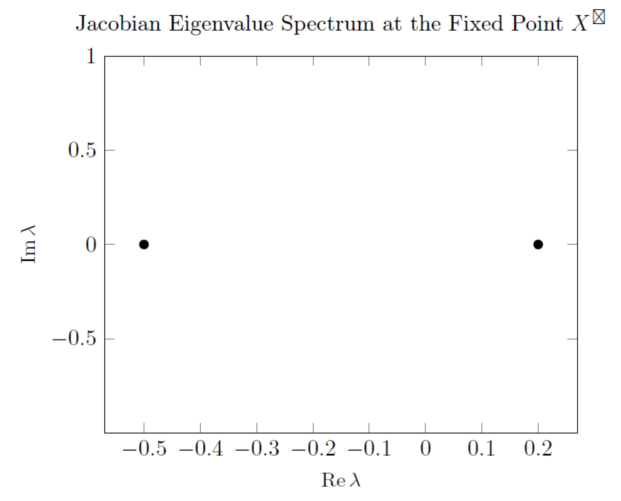
Figure 3.
Phase-transition lines and a multicritical point in a multi-coupling system (example)
Figure 4.
Two–loop evolution of : SM (dashed) vs. UEE–SU(5) (solid). Even with dissipative corrections for TeV the crossing point is stable within dex.
Figure 4.
Two–loop evolution of : SM (dashed) vs. UEE–SU(5) (solid). Even with dissipative corrections for TeV the crossing point is stable within dex.
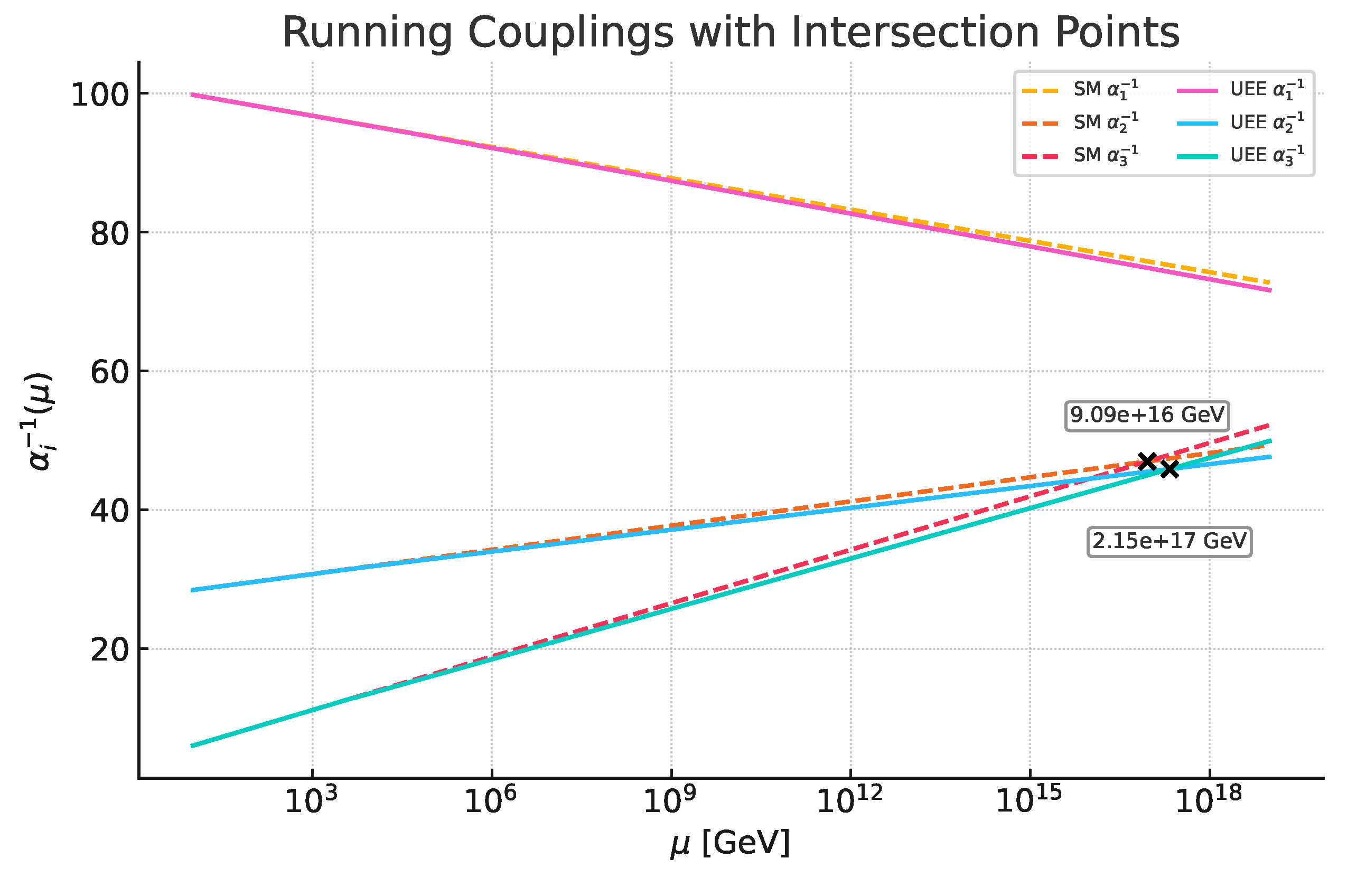
Figure 5.
FRGE flow in the -plane. The black dot marks the non-trivial fixed point (7.2.1) [299]; blue arrows indicate the UV → IR direction.
Figure 5.
FRGE flow in the -plane. The black dot marks the non-trivial fixed point (7.2.1) [299]; blue arrows indicate the UV → IR direction.
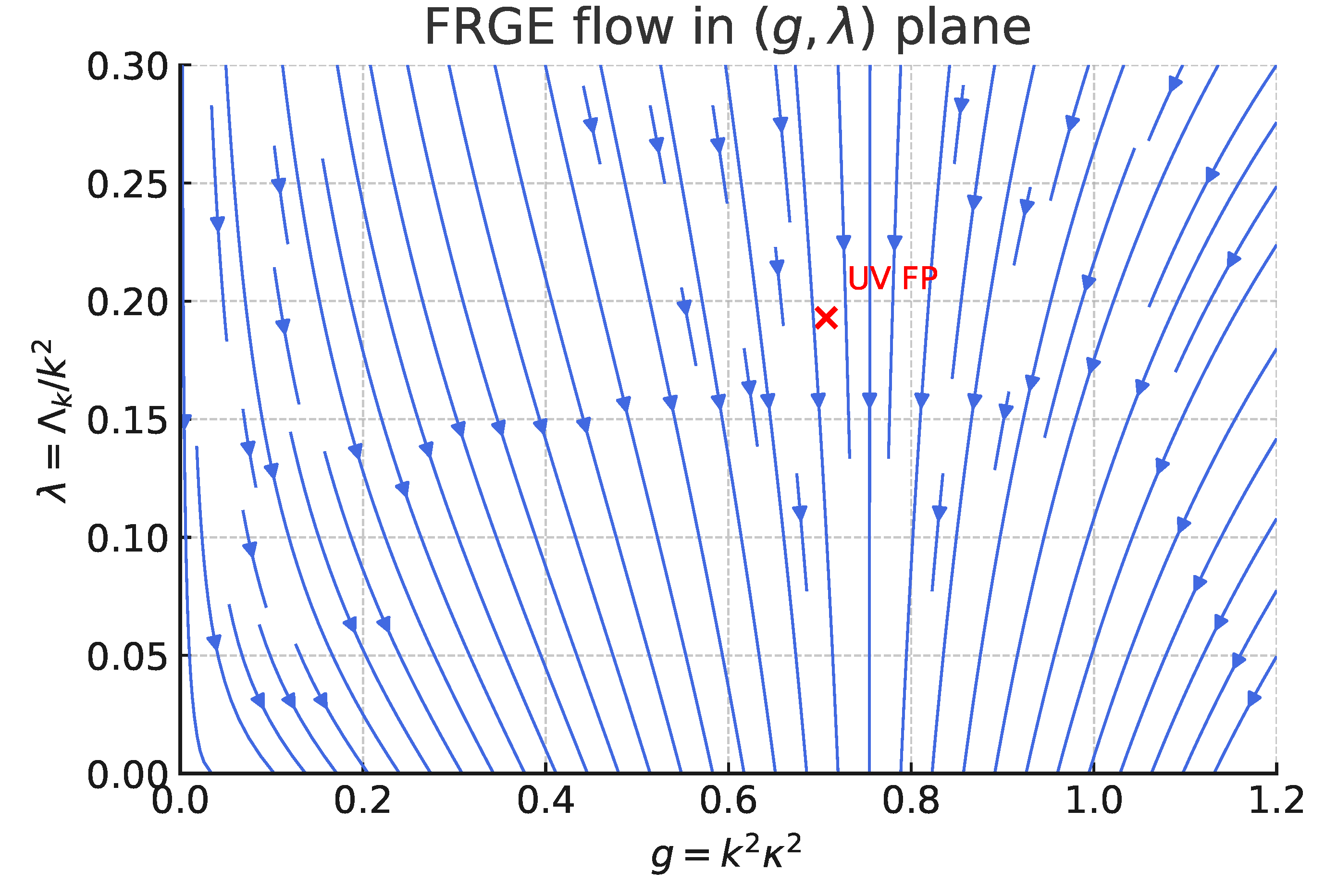
Figure 6.
RG running of the dissipative strength . It converges to in the UV and keeps the relative-boundedness condition [24].
Figure 6.
RG running of the dissipative strength . It converges to in the UV and keeps the relative-boundedness condition [24].
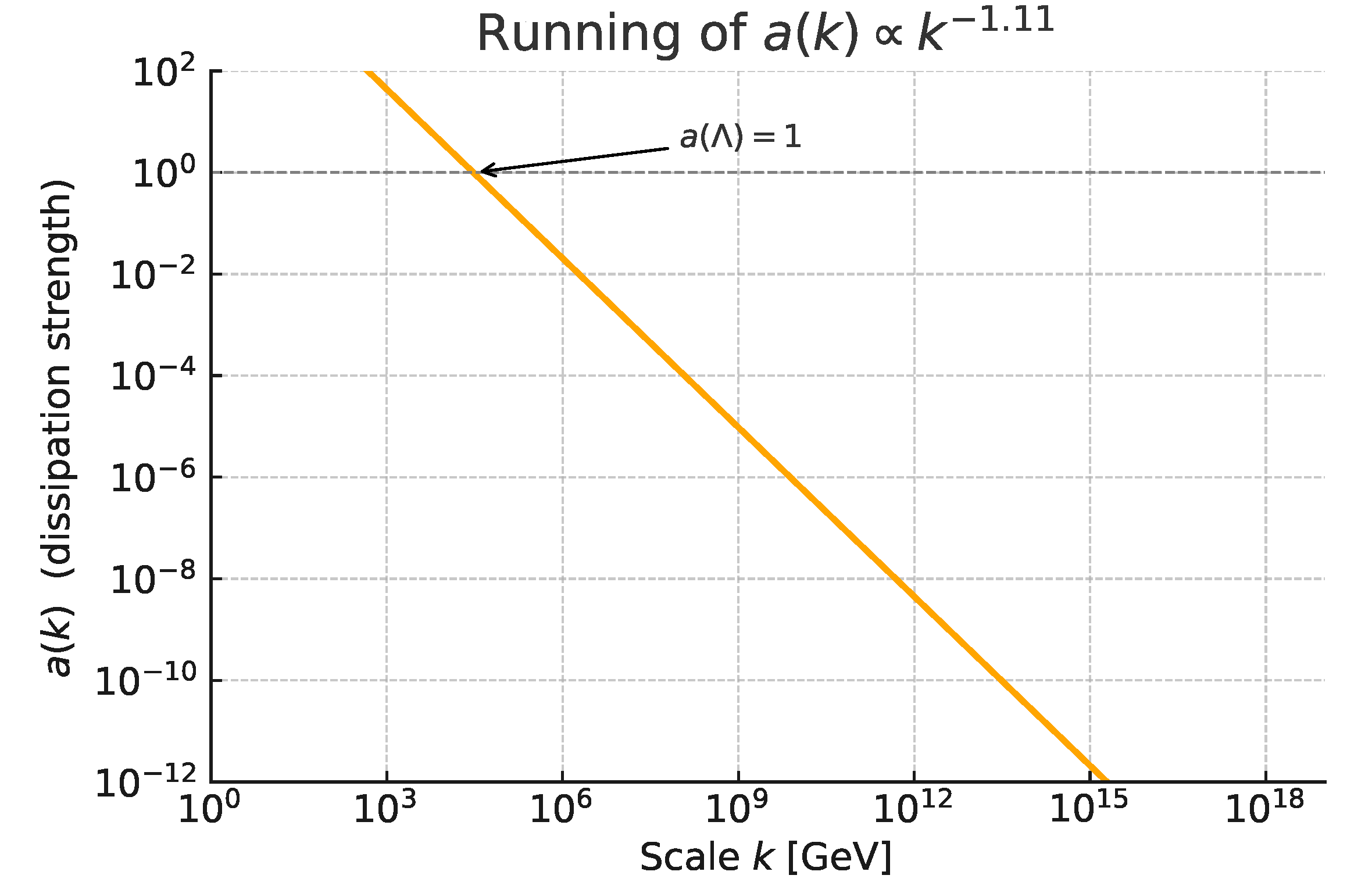
Table 2.
Lower bound after adding a mass term . (The mass parameter is assumed to satisfy with the physical cut-off .)
Table 2.
Lower bound after adding a mass term . (The mass parameter is assumed to satisfy with the physical cut-off .)
| Corresponding maximal | ||
|---|---|---|
| 1 | 1 |
Table 5.
Key parameters and their CL ranges (two–loop RG running + proton decay + neutrino masses).
| Parameter | Preferred central value | CL interval |
|---|---|---|
| (GeV) | – | |
| 37.2 | 34.5 – 39.5 | |
| 0.63 | 0.55 – 0.75 | |
| 3.2 | 1.5 – 6.0 | |
| (GeV) | – | |
| (TeV) |
Table 6.
Posterior parameters ( CL).
| Parameter | UEE mean | CDM mean |
|---|---|---|
| (95% CL) | — | |
| — |
Disclaimer/Publisher’s Note: The statements, opinions and data contained in all publications are solely those of the individual author(s) and contributor(s) and not of MDPI and/or the editor(s). MDPI and/or the editor(s) disclaim responsibility for any injury to people or property resulting from any ideas, methods, instructions or products referred to in the content. |
© 2025 by the authors. Licensee MDPI, Basel, Switzerland. This article is an open access article distributed under the terms and conditions of the Creative Commons Attribution (CC BY) license (http://creativecommons.org/licenses/by/4.0/).
Copyright: This open access article is published under a Creative Commons CC BY 4.0 license, which permit the free download, distribution, and reuse, provided that the author and preprint are cited in any reuse.


