
Submitted:
26 April 2025
Posted:
29 April 2025
You are already at the latest version
Abstract
A common approach to estimate the spatial-temporal distribution of atmospheric species properties is data assimilation. Data assimilation methods provide the best estimate of the required parameter by combining observations with appropriate prior information (background) that can be model output, climatology, or some other first guess. One of the relatively simple and computationally cheap data assimilation methods is optimal interpolation (OI). It estimates a value of interest through a weighted linear combination of observational data and background that is defined only once for the whole time interval of interest. Spatial-temporal OI (STOI) utilizes both spatial and temporal observational error covariance and background error covariance. This allows for filling in not only spatial, but also temporal gaps in observations. We applied STOI to daily mean aerosol optical depth (AOD) observations obtained at the European AERONET (Aerosol Robotic Network) sites with the use of the GEOS-Chem chemical transport model simulations and the AOD climatology as backgrounds. We found that mean square errors in the estimate when using modeled data are comparable with those when using climatology. Based on these results, we merged estimates obtained using modeled data and climatology according to their mean square errors. This allows improving AOD estimates in areas where observations are limited in space and time.
Keywords:
data assimilation
; spatial-temporal optimal interpolation
; aerosol optical depth
; chemical transport model GEOS-Chem
; radiometric network AERONET
1. Introduction
Studying the composition of the Earth's atmosphere is crucial for understanding climate change and predicting air quality. The state of the atmosphere is monitored using various in situ and remote sensing observations. However, there can be significant differences in data obtained using different instruments and techniques. Observations can be irregular, sparse in space, with different uncertainties. To estimate atmospheric characteristics on some regular spatial-temporal grid, data assimilation [1,2,3,4,5] is commonly applied. The goal of data assimilation is to minimize on average the difference between the estimate of the system state and the true system state.
Data assimilation comprises methods that merge information from different sources for obtaining the best estimate of the system state. The mathematical basis for data assimilation is estimation theory [6,7]. In a data assimilation scheme, observations are combined with some prior information, or background, that provides a first guess estimate. The background represents the best estimate of the true state available before observations are made. In atmospheric science, the background is often chosen to be a model output or climatology represented on some discrete grid. The information contained in observational data is spread in space using background error correlations.
Data assimilation methods are historically divided into optimal interpolation (OI) [8,9], Kalman filtering (KF) [10,11], variational 3-dimentional (3D-Var) [12,13] and 4-dimentional (4D-Var) [14,15] methods. Under common assumptions of linearity and Gaussian errors probability distribution, 3D-Var methods differ from OI, and 4D-Var methods differ from KF only by the mathematical approach to the solution [4,5,16,17]. OI and 3d-Var methods are non-sequential. Non-sequential assimilation uses the background, which is defined only once for the whole time interval of interest. KF and 4d-Var methods are sequential. In sequential assimilation, the background is given by the model forecast, starting from the estimate at the previous time step. The background and its error variance are updated at every time step, so sequential methods in general provide lower mean square error of the estimate [18]. In sequential methods, the trajectory of the estimated system state contains discontinuities whenever a new observation is encountered [19], so these methods are not well suited for retrospective analysis. Sequential assimilation needs to be regularly fed with observations. Otherwise the system returns to the model trajectory within a relatively small time interval, and sequential methods do not provide better performance than non-sequential [2,20].
Among data assimilation methods, OI is the simplest and the less computationally costly [4,11,18]. OI is one of the easiest ways to perform data assimilation. This method is rather data fusion. To produce the estimate, OI merges observations and a background, which is defined only once for the whole time interval of interest.
Being a non-sequential method, OI can benefit from a possibility to use not only spatial, but also temporal correlation. In previous works we developed a spatial-temporal optimal interpolation (STOI) method [21,22]. This is an extended OI method in which time dimension is added by using correlations in time in addition to correlations in space. STOI allows for filling in not only spatial, but also temporal gaps in observations. This makes STOI particularly useful for the assimilation of temporally sparse observations. STOI is а simple to implement and computationally cheap method that shows accuracy comparable with other assimilation methods when using observational data with large temporal gaps. STOI is suitable for a retrospective analysis. Due to using temporal correlations, the system trajectory is smooth in time that provides a physically more realistic picture of a spatial-temporal distribution of atmospheric species characteristics. These are the reasons for developing STOI in the application to observations limited in space and time, such as optical remote sensing observations.
One of the important atmospheric characteristics obtained using optical remote sensing is aerosol optical depth (AOD).
AOD is an aerosol optical quantity that reflects the column-integrated atmospheric aerosol amount. A number of actual problems require knowing a spatial-temporal distribution of AOD. Various atmospheric aerosol properties can be derived from AOD observations [23,24]. In the last decades, numerous studies were dedicated to the estimation of AOD distribution using different data assimilation approaches [25,26,27] including OI [28,29,30]. However, only spatial OI was considered.
In [22] we showed that STOI provides an improvement in AOD estimates. The present paper is dedicated to further improvement of the STOI accuracy. The choice of the background can significantly affect the result of the estimation. In the early OI methods, the climatology was used as a background [8]. Later the climatology was replaced with the model output. We wondered if the model output is much better than the climatology when using as a background for the AOD assimilation. In the present study, we applied the STOI technique to AOD observations using a chemical transport model simulations and climatology as backgrounds. We compared results obtained using these two backgrounds, and proposed an approach to STOI that uses both modeled data and climatology as backgrounds according to their mean square errors.
The paper is organized as follows. In section 2 we described the STOI technique, AOD observations and background fields used in the assimilation process, in section 3 we evaluated and discussed the proposed approach to the AOD estimation, and drew conclusions.
2. Materials and Methods
Spatial-temporal optimal interpolation method is based on the classical OI. It uses common equations of optimal estimation theory [4,17]:
were xa is a vector containing estimates of the state of the system, xb is a vector containing background values, y is a vector containing values of observations, K is a matrix containing weighting coefficients, H is an observation operator (observation model) providing the link between the observations and variables describing the state of the system, B is a covariance matrix of background errors, and R is a covariance matrix of observational errors. The matrix of weighting coefficients, K, is to be determined by minimizing the mean-square error in the estimate. In OI, the estimates are obtained for each grid point independently with weighting coefficients determined at each grid point. The estimate at a particular grid point is obtained as the sum of the background value at the point of estimation, and the estimation increment (deviation of the estimate from the background). After transforming the vector of observations into the same type of variables as the background (or if observational and background variables are the same), the estimation increment is calculated as a weighted linear combination of the anomalies (deviations of the observations from the background) at the neighboring observational points. Only a limited number of observations are taking into consideration in the vicinity of the point of estimation. In the absence of observational data and outside the background error correlation area, the background is considered as the best estimate of a system state.
In the OI scheme, background and observational errors are assumed to be unbiased, observational errors to be uncorrelated, background and observational errors to be mutually uncorrelated. Another common assumption is that the background error correlation is homogeneous and isotropic.
In STOI not only observations at the time point of estimation, but also observations at the neighboring time points are used, assuming homogeneity and isotropy in time.
We applied STOI to daily mean AOD observations from a global radiometric ground-based Aerosol Robotic Network (AERONET) [31,32,33]. AERONET utilizes Cimel multi-channel, automatic sun-sky-lunar scanning photometers CE318 designed for automatic multispectral atmospheric photometry [34]. The measurements of direct solar and lunar, and diffused sky radiance are performed at a number of wavelengths in the range 340–1640 nm. AOD is derived from AERONET radiance measurements using retrieval algorithm [35]. AOD and other aerosol optical, microphysical and radiative properties are displayed in the AERONET website [36]. An uncertainty of AERONET observations of AOD is estimated to be 0.01 for wavelengths > 440 nm [37,38]. We used version 3 AERONET Level 2.0 cloud-screened and quality-assured daily averaged total AOD data at wavelengths of 440, 675, and 870 nm.
We performed STOI using observations from the 86 European AERONET sites for the period of two years from 1 January 2015 to 31 December 2016. Table A1 lists the AERONET sites used in the study along with their geographic location. We used two different backgrounds: climatology and results of a chemical transport model simulation.
We obtained the climatology background by averaging AOD values at abovementioned AERONET sites. This approach is clearly crude, and in future we plan to build more relevant climatology background.
We obtained a modeled background by calculations with the GEOS-Chem chemical transport model [39,40,41]. This model is continuously updated and widely used by the air quality community. GEOS-Chem simulates the evolution of more than two hundred atmospheric species including aerosols. We used the version v12.1.1 of GEOS-Chem in the classical configuration (GEOS-Chem Classic) in the off-line mode, in which the model is driven by archived meteorological observations from the Goddard Earth Observing System (GEOS) of the NASA Global Modeling and Assimilation Office [42]. GEOS-Chem uses the Harvard–NASA Emissions Component (HEMCO) [43] for computing atmospheric emissions from different inventories. The advection algorithm of CEOS-Chem Classic was described in [44]. The oxidant-aerosol chemistry in the troposphere and stratosphere was described in [45,46,47]. When calculating AOD, the aerosol types in GEOS-Chem are categorized into groups according to their optical properties: sulfate–nitrate–ammonium; size fractions of mineral dust; sea salt in accumulation and coarse modes; black carbon; organic aerosols. Aerosol optical properties are from [48,49]. The hygroscopic growth is taken into account.
GEOS-Chem allows simulations in global and regional scales. The nested capability for CEOS-Chem Classic was implemented by [50,51,52]. The nested European domain in GEOS-Chem is 32.75°N–61.25°N, 15°W–40°E.
We simulated daily averaged AOD at 440, 675, and 870 nm for the European domain at 0.25° latitude × 0.3125° longitude horizontal resolution and 47 vertical σ-layers up to ~80 km. For performing nested simulation we used boundary conditions from the global simulation at 2° latitude × 2.5° longitude horizontal resolution.
The AOD uncertainty obtained with a model simulation is significantly larger than retrieved from AERONET measurements [53,54], so we assumed the AERONET AOD uncertainty to be negligible. This assumption allows calculating background covariances using differences between the observational and background values. As the correlation structure of the background errors is assumed to be homogeneous and isotropic, the correlation function is the same for any spatial-temporal point and in any direction. We modeled spatial and temporal correlation coefficients by exponential functions on the basis of calculated spatial and temporal covariances.
3. Results and Discussion
Obtained spatial and temporal correlation functions for GEOS-Chem output and climatology as backgrounds are shown in Figure 1.
Correlation functions are almost similar for both model and climatology errors in AOD estimate. Correlation curves for climatology lie slightly higher than for model output. Such behavior can be explained by higher imperfection of climatology.
To evaluate the efficiency of STOI when using model output and climatology as backgrounds, we compared the estimates against observations that were not used in data assimilation. We chose Lille, Minsk, and Granada AERONET sites to exclude from the data assimilation process, same as in our previous article [22]. We calculated root-mean-square errors (RMSE) of the estimates for model output and climatology backgrounds. The results are presented in Table 1 (using GEOS-Chem output as the background) and Table 2 (using climatology as the background). In parentheses, the reduction in RMSE of the estimate after STOI is shown in tables.
The comparison shows that RMSE in the STOI estimate of AOD when using modeled data as background do not differ significantly from those when using climatology. This indicates that AOD calculations are prone to large errors. The difference in RMSE is larger in Lille than in Granada because the area where Granada site is located is rich in AERONET sites and sunny days. Minsk shows the largest difference in RMSE due to sparse distribution of AERONET sites in this area and predominance of cloudy days. It is obvious that far from spatial-temporal observation points the background plays more important role.
The results of the comparison of RMSE in Table 1 and Table 2 imply the possibility of using climatology as background instead of model output for AERONET AOD assimilation. This greatly reduces computational cost. On the base of the obtained results we assumed that RMSE in the STOI estimate of AOD can probably be decreased by using both model results and climatology as backgrounds with weighting coefficients according to RMSE of these fields. The second background would provide additional independent information and therefore enhance the accuracy of the estimate.
The results of merging the AOD estimates obtained using both model output and climatology are shown in Table 3.
It can be seen from the Table 3 in comparison with Table 1 and Table 2 that using two backgrounds does not affect the results for Granada, slightly improves the results for Lille, and significantly improves the results for Minsk. This is in agreement with statements of the data assimilation theory that the background makes the main contribution to the estimate far from observations.
Therefore, the proposed approach has the potential to improve the estimate of atmospheric species characteristics distribution when observations are sparse.
The main conclusions are as follows. The present study confirms a capability of STOI to fill in spatial and temporal gaps in observations. The STOI estimates are sensitive to the choice of the background in areas with sparsely distributed observations. Using both model output and climatology as backgrounds allows reducing uncertainty in the estimate in areas where observations are limited in space and time without significant increasing the computational cost.
In future we plan to apply the developed approach to the estimation and analysis of spatial distribution and temporal variation of atmospheric species over certain regions of interest.
Author Contributions
Conceptualization, N.M. and A.C.; methodology, N.M.; software, N.M. and A.B.; validation, N.M. and A.B.; investigation, N.M.; data curation, N.M., A.B. and A.C., writing—original draft preparation, N.M.; writing—review and editing, A.B. and A.C.; visualization, N.M. All authors have read and agreed to the published version of the manuscript.
Funding
This research received no external funding.
Institutional Review Board Statement
Not applicable.
Informed Consent Statement
Not applicable.
Data Availability Statement
AERONET data are freely available from https://aeronet.gsfc.nasa.gov (accessed on 16 April 2025). GEOS-Chem simulation and the STOI data generated in this work are freely available from http://scat.bas-net.by/~assimilation/ (accessed on 16 April 2025).
Conflicts of Interest
The authors declare no conflicts of interest.
Abbreviations
The following abbreviations are used in this manuscript:
| AOD | Aerosol optical depth |
| OI STOI KF 3D-Var 4D-Var |
Optimal interpolation Spatial-temporal optimal interpolation Kalman filtering 3-dimentional variational 4-dimentional variational |
| AERONET | Aerosol Robotic Network |
| RMSE | Root-mean-square error |
Appendix A

Table A1.
AERONET sites taken into account when performing STOI and their geographic location as presented at AERONET website [36].
Table A1.
AERONET sites taken into account when performing STOI and their geographic location as presented at AERONET website [36].
| AERONET site | Longitude | Latitude |
|---|---|---|
| Lille Barcelona Venise Xanthi Ispra Mainz Helgoland Palaiseau Paris Moldova IMS-METU-ERDEMLI Kyiv Hamburg Modena Moscow_MSU_MO Minsk Rome_Tor_Vergata Leipzig Davos Munich_University Lecce_University ATHENS-NOA Belsk Villefranche Palencia Carpentras Toulon Dunkerque Evora Laegeren Cabo_da_Roca Granada Gustav_Dalen_Tower OHP_OBSERVATOIRE Chilbolton Helsinki_Lighthouse Sevastopol Brussels Zvenigorod Porquerolles Burjassot Bucharest_Inoe Autilla Kanzelhohe_Obs Ersa Arcachon Wytham_Woods Malaga Birkenes Eforie Huelva Aubiere_LAMP Frioul CLUJ_UBB Gloria Bari_University Tabernas_PSA-DLR Calern_OCA Montsec Bure_OPE Coruna Madrid Tizi_Ouzou Iasi_LOASL Zaragoza FZJ-JOYCE Badajoz Cerro_Poyos Valladolid Murcia MetObs_Lindenberg Ben_Salem CENER HohenpeissenbergDWD Galata_Platform Tunis_Carthage Carloforte Exeter_MO Strzyzow LAQUILA_Coppito Toulouse_MF Martova Zeebrugge-MOW1 Peterhof Finokalia-FKL Berlin_FUB |
3.142°E 2.112°E 12.508°E 24.919°E 8.627°E 8.3°E 7.887°E 2.215°E 2.356°E 28.816°E 34.255°E 30.497°E 9.973°E 10.945°E 37.522°E 27.601°E 12.647°E 12.435°E 9.844°E 11.573°E 18.111°E 23.718°E 20.792°E 7.329°E 4.516°W 5.058°E 6.009°E 2.368°E 7.911°W 8.364°E 9.498°W 3.605°W 17.467°E 5.71°E 1.437°W 24.926°E 33.517°E 4.35°E 36.775°E 6.161°E 0.42°W 26.028°E 4.603°W 13.901°E 9.359°E 1.163°W 1.332°W 4.478°W 8.252°E 28.632°E 6.569°W 3.111°E 5.293°E 23.551°E 29.36°E 16.884°E 2.358°W 6.923°E 0.73°E 5.505°E 8.421°W 3.724°W 4.056°E 27.556°E 0.882°W 6.413°E 7.011°W 3.487°W 4.706°W 1.171°W 14.121°E 9.914°E 1.602°W 11.012°E 28.193°E 10.2°E 8.31°E 3.475°W 21.861°E 13.351°E 1.374°E 36.953°E 3.12°E 29.826°E 25.67°E 13.31°E |
50.612°N 41.389°N 45.314°N 41.147°N 45.803°N 49.999°N 54.178°N 48.712°N 48.847°N 47.001°N 36.565°N 50.364°N 53.568°N 44.632°N 55.707°N 53.92°N 41.84°N 51.353°N 46.813°N 48.148°N 40.335°N 37.972°N 51.837°N 43.684°N 41.989°N 44.083°N 43.136°N 51.035°N 38.568°N 47.478°N 38.782°N 37.164°N 58.594°N 43.935°N 51.144°N 59.949°N 44.616°N 50.783°N 55.695°N 43.001°N 39.507°N 44.348°N 41.997°N 46.677°N 43.004°N 44.664°N 51.77°N 36.715°N 58.388°N 44.075°N 37.016°N 45.761°N 43.266°N 46.768°N 44.6°N 41.108°N 37.091°N 43.752°N 42.051°N 48.562°N 43.363°N 40.452°N 36.699°N 47.193°N 41.633°N 50.908°N 38.883°N 37.109°N 41.664°N 38.001°N 52.209°N 35.551°N 42.816°N 47.802°N 43.045°N 36.839°N 39.14°N 50.729°N 49.879°N 42.368°N 43.573°N 49.936°N 51.362°N 59.881°N 35.338°N 52.458°N |
References
- Lahoz, W.A. Data Assimilation; Springer-Verlag Berlin Heidelberg, 2010.
- Sandu, A.; Chai, T. Chemical Data Assimilation — An Overview. Atmosphere 2011, 2, 426–463. [CrossRef]
- Bocquet, M.; Elbern, H.; Eskes, H.; Hirtl, M.; Žabkar, R.; Carmichael, G.R.; Flemming, J.; Inness, A.; Pagowski, M.; Pérez Camaño, J.L.; Saide, P.E.; San Jose, R.; Sofiev, M.; Vira, J.; Baklanov, A.; Carnevale, C.; Grell, G.; C. Seigneur, C. Data Assimilation in Atmospheric Chemistry Models: Current Status and Future Prospects for Coupled Chemistry Meteorology Models. Atmos. Chem. Phys. 2015, 15, 5325–5358. [CrossRef]
- Kalnay, E. Atmospheric Modeling, Data Assimilation and Predictability; Cambridge University Press: Cambridge, UK, 2002.
- Wikle, C.K.; Berliner, L.M. A Bayesian Tutorial for Data Assimilation. Phys. D. Nonlinear Phenom. 2007, 230, 1–16. https://doi:10.1016/j.physd.2006.09.017.
- Daley, R. Atmospheric Data Analysis; Cambridge University Press: Cambridge, UK, 1991.
- Rodgers, C. D. Inverse Methods for Atmospheric Sounding : Theory and Practice; World Scientific: Singapore, 2000.
- Gandin, L.S. Objective Analysis of Meteorological Fields; Gidrometeorol. Izd.: Leningrad, Russia, 1963.
- Lorenc, A.C. A Global Three-Dimensional Multivariate Statistical Analysis Scheme. Mon. Weather Rev. 1981, 109, 701–721. [CrossRef]
- Kalman, R.E. A New Approach to Linear Filtering and Prediction Problems. J. Basic Eng. 1960, 82, 35–45. [CrossRef]
- Constantinescu, E.M.; Sandu, A.; Chai, T.; Carmichael, G. Ensemble-based Chemical Data Assimilation: General Approach. Q. J. R. Meteorol. Soc. 2007, 133, 1229–1243. [CrossRef]
- Sasaki, Y. An Objective Analysis Based on the Variational Method. J. Meteorol. Soc. Japan 1958, 36, 77–88. [CrossRef]
- Le Dimet, F.-X.; Talagrand, O. Variational Algorithms for Analysis and Assimilation of Meteorological Observations: Theoretical Aspects. Tellus 1986, 38A, 97–110. [CrossRef]
- Courtier, P.; Thepaut, J.-N.; Hollingsworth, A. A Strategy for Operational Implementation of 4D-Var, Using an Incremental Approach. Q. J. R. Meteorol. Soc. 1994, 120, 1367–1387. [CrossRef]
- Carmichael, G.R.; Sandu, A.; Chai, T.; Daescu, D.N.; Constantinescu, E.M;, Tang, Y. Predicting Air Quality: Improvements through Advanced Methods to Integrate Models and Measurements. J. Comput. Phys., 2008, 227, 3540–3571. [CrossRef]
- Wahba, G.; Wendelberger, J. Some New Mathematical Methods for Variational Objective Analysis Using Splines and Cross Validation. Mon. Wea. Rev. 1980, 108, 1122–1143.
- Lorenc, A.C. Analysis Methods for Numerical Weather Prediction. Q. J. R. Meteorol. Soc. 1986, 112, 1177–1194. [CrossRef]
- Candiani, G.; Carnevale, C.; Finzi, G.; Pisoni, E.; Volta, M. A Comparison of Reanalysis Techniques: Applying Optimal Interpolation and Ensemble Kalman Filtering to Improve Air Quality Monitoring at Mesoscale. Sci. Total Environ. 2013, 458–460, 7–14. [CrossRef]
- Khattatov, B.V.; Gille, J.C.; Lyjak, L.V.; Brasseur, G.P.; Dvortsov, V.L.; Roche, A.E.; Waters, J. Assimilation of Photochemically Active Species and a Case Analysis of UARS Data. J. Geophys. Res. 1999, 104, 18715–18737. http://dx.doi.org/10.1029/1999JD900225.
- Tombette, M.; Mallet, V.; Sportisse, B. PM10 Data Assimilation over Europe with the Optimal Interpolation Method. Atmos. Chem. Phys. 2009, 9, 57–70. [CrossRef]
- Miatselskaya, N.S.; Bril, A.I.; Chaikovsky, A.P.; Yukhymchuk, Yu.Yu.; Milinevski, G.P.; Simon, A.A. Optimal Interpolation of AERONET Radiometric Network Observations for the Evaluation of the Aerosol Optical Thickness Distribution in the Eastern European Region. J. Appl. Spectrosc. 2022, 89, 296–302. [CrossRef]
- Miatselskaya, N.; Milinevsky, G.; Bril, A.; Chaikovsky, A.; Miskevich, A.; Yukhymchuk, Y. Application of Optimal Interpolation to Spatially and Temporally Sparse Observations of Aerosol Optical Depth. Atmosphere. 2023, 14, 32. [CrossRef]
- Donkelaar, A.; Martin, R.V.; Park, R.J. Estimating Ground-level PM2.5 with Aerosol Optical Depth Determined from Satellite Remote Sensing. J. Geophys. Res. 2006, 111, D21201. [CrossRef]
- Perez-Ramirez, D.; Veselovskii, I.; Whiteman, D. N.; Suvorina, A.; Korenskiy, M.; Kolgotin, A.; Holben, B.; Dubovik, O.; Siniuk, A.; Alados-Arboledas, L. High Temporal Resolution Estimates of Columnar Aerosol Microphysical Parameters from Spectrum of Aerosol Optical Depth by Linear Estimation: Application to Long-term AERONET and Star-photometry Measurements. Atmos. Meas. Tech., 2015, 8, 3117–3133. [CrossRef]
- Yu, H.; Dickinson, R.E.; Chin, M.; Kaufman, Y.J.; Geogdzhayev, B.; Mishchenko, M.I. Annual Cycle of Global Distributions of Aerosol Optical Depth from Integration of MODIS Retrievals and GOCART Model Simulations. J. Geophys. Res. 2003, 108, 4128. [CrossRef]
- Adhikary, B.; Kulkarni, S.; Dallura, A.; Tang, Y.; Chai, T.; Leung, L.R.; Qian, Y.; Chung, C.E.; Ramanathan, V.; Carmichael, G.R. A Regional Scale Chemical Transport Modeling of Asian Aerosols with Data Assimilation of AOD Observations Using Optimal Interpolation Technique. Atmos. Env. 2008, 42, 8600–8615. [CrossRef]
- Rubin, J.I.; Reid, J.S.; Hansen, J.A.; Anderson, J.L.; Holben, B.N.; Xian, P.; Westphal, D.L.; Zhang, J. Assimilation of AERONET and MODIS AOT Observations Using Variational and Ensemble Data Assimilation Methods and Its Impact on Aerosol Forecasting Skill. J. Geophys. Res.–Atmos. 2017, 122, 4967–4992. [CrossRef]
- Collins, W.D.; Rasch, P.J.; Eaton, B.E.; Khattatov, B.V.; Lamarque, J.-F.; Zender, C.S. Simulating Aerosols Using a Chemical Transport Model with Assimilation of Satellite Aerosol Retrievals: Methodology for INDOEX. J. Geophys. Res. Atmos. 2001, 106, 7313–7336. [CrossRef]
- Xue, Y.; Xu, H.; Guang, J.; Mei, L.; Guo, J.; Li, C.; Mikusauskas, R.; He, X. Observation of an Agricultural Biomass Burning in Central and East China Using Merged Aerosol Optical Depth Data from Multiple Satellite Missions. Int. J. Remote Sens. 2014, 35, 5971-5983. [CrossRef]
- Li, K.; Bai, K.; Li, Z.; Guo, J.; Chang, N.-B. Synergistic Data Fusion of Multimodal AOD and Air Quality Data for Near Real-Time Full Coverage Air Pollution Assessment. J. Environ. Manag. 2022, 302, 114121. [CrossRef]
- Holben, B.N.; Eck, T.F.; Slutsker, I.; Tanre, D.; Buis, J.P.; Setzer, A.; Vermote, E.; Reagan, J.A.; Kaufman, Y.J.; Nakajima, T.; et al. AERONET—A Federated Instrument Network and Data Archive for Aerosol Characterization. Remote Sens. Environ. 1998, 66, 1–16. [CrossRef]
- Holben, B.N.; Kim, J.; Sano, I.; Mukai, S.; Eck, T.F.; Giles, D.M.; Schafer, J.S.; Sinyuk, A.; Slutsker, I.; Smirnov, A. An Overview of Mesoscale Aerosol Processes, Comparisons, and Validation Studies from DRAGON Networks. Atmos. Chem. Phys. 2018, 18, 655–671. [CrossRef]
- Giles, D.M.; Sinyuk, A.; Sorokin, M.G.; Schafer, J.S.; Smirnov, A.; Slutsker, I.; Eck, T.F.; Holben, B.N.; Lewis, J.R.; Campbell, J.R.; Welton, E.J.; Korkin, S.V.; Lyapustin, A.I. Advancements in the Aerosol Robotic Network (AERONET) Version 3 Database – Automated Near-Real-Time Quality Control Algorithm with Improved Cloud Screening for Sun Photometer Aerosol Optical Depth (AOD) Measurements. Atmos. Meas. Tech. 2019, 12, 169–209, . [CrossRef]
- Available online: https://www.cimel.fr/ (accessed on 10 April 2025).
- Dubovik, O.; King, M.D. A Flexible Inversion Algorithm for Retrieval of Aerosol Optical Properties from Sun and Sky Radiance Measurements. J. Geophys. Res. 2000, 105, 20673–20696. [CrossRef]
- Available online: https://aeronet.gsfc.nasa.gov/ (accessed on 16 April 2025).
- Eck, T.F.; Holben, B.N.; Reid, J.S.; Dubovik, O.; Smirnov, A.; O’Neill, N.T.; Slutsker, I.; Kinne, S. Wavelength Dependence of the Optical Depth of Biomass Burning, Urban and Desert Dust Aerosols. J. Geophys. Res. 1999, 104, 31333–31349. [CrossRef]
- Holben, B.N.; Tanre, D.; Smirnov, A.; Eck, T.F.; Slutsker, I.; Abuhassan, N.; Newcomb, W.W.; Schafer, J.; Chatenet, B.; Lavenue, F.; Kaufman, Y.J.; Vande Castle, J.; Setzer, A.; Markham, B.; Clark, D.; Frouin, R.; Halthore, R.; Karneli, A.; O'Neill, N.T.; Pietras, C.; Pinker, R.T.; Voss, K.; Zibordi, G. An Emerging Ground-Based Aerosol Climatology: Aerosol Optical Depth from AERONET. J. Geophys. Res. 2001, 106, 12067–12097. [CrossRef]
- Available online: https://geoschem.github.io (accessed on 10 April 2025).
- Bey, I.; Jacob, D.J.; Yantosca, R.M.; Logan, J.A.; Field, B.D.; Fiore, A.M.; Li, Q.; Liu, H.Y.; Mickley, L.J.; Schultz, M.G. Global Modeling of Tropospheric Chemistry with Assimilated Meteorology: Model Description and Evaluation. J. Geophys. Res. 2001, 106, 23073–23096. [CrossRef]
- Park, R.J.; Jacob, D.J.; Field, B.D.; Yantosca, R.M.; Chin, M. Natural and Transboundary Pollution Influences on Sulfate-Nitrate-Ammonium Aerosols in the United States: Implications for Policy. J. Geophys. Res. 2004, 109, D15204. [CrossRef]
- Available online: https://gmao.gsfc.nasa.gov/GEOS_systems/ (accessed on 16 April 2025).
- Keller, C.A.; Long, M.S.; Yantosca, R.M.; Da Silva, A.M.; Pawson, S.; Jacob, D.J. HEMCO v1.0: A Versatile, ESMF-Compliant Component for Calculating Emissions in Atmospheric Models. Geosci. Model Dev. 2014, 7, 1409–1417. [CrossRef]
- Lin, S.-J.; Rood, R.B. Multidimensional Flux Form Semi-Lagrangian Transport Schemes. Mon. Weather Rev. 1996, 124, 2046–2070.
- Sherwen, T.; Schmidt, J.A.; Evans, M.J.; Carpenter, L.J.; Grossmann, K.; Eastham, S.D.; Jacob, D.J.; Dix, B.; Koenig, T.K.; Sinreich, R.; Ortega, I.; Volkamer, R.; Saiz-Lopez, A.; Prados-Roman, C.; Mahajan, A.S.; Ordóñez, C. Global Impacts of Tropospheric Halogens (Cl, Br, I) on Oxidants and Composition in GEOS-Chem. Atmos. Chem. Phys. 2016, 16, 12239–12271. [CrossRef]
- Travis, K.R.; Jacob, D.J.; Fisher, J.A.; Kim, P.S.; Marais, E.A.; Zhu, L.; Yu, K.; Miller, C.C.; Yantosca, R.M.; Sulprizio, M.P.; Thompson, A.M.; Wennberg, P.O.; Crounse, J.D.; St. Clair, J.M.; Cohen, R.C.; Laughner, J.L.; Dibb, J.E.; Hall, S.R.; Ullmann, K.; Wolfe, G.M.; Pollack, I.B.; Peischl, J.; Neuman, J.A.; Zhou, X. Why Do Models Overestimate Surface Ozone in the Southeast United States? Atmos. Chem. Phys. 2016, 16, 13561–13577, . [CrossRef]
- Eastham, S.D.; Weisenstein, D.K.; Barrett, S.R.H. Development and Evaluation of the Unified Tropospheric–Stratospheric Chemistry Extension (UCX) for the Global Chemistry-Transport Model GEOS-Chem. Atmos. Environ. 2014, 89, 52–63. [CrossRef]
- Latimer, R.N.C.; Martin, R.V. Interpretation of Measured Aerosol Mass Scattering Efficiency over North America Using a Chemical Transport Model. Atmos. Chem. Phys. 2019, 19, 2635–2653. [CrossRef]
- Ridley, D.A.; Heald, C.L.; Ford, B. North African Dust Export and Deposition: A Satellite and Model Perspective. J. Geophys. Res. 2012, 117, D02202. [CrossRef]
- Wang, Y.X.; Mcelroy, M.B.; Jacob, D.J.; Yantosca, R.M. A Nested Grid Formulation for Chemical Transport over Asia: Applications to CO. J. Geophys. Res. Atmos. 2004, 109, D22307. 10.1029/2004JD005237.
- Zhang, L.; Liu, L.; Zhao, Y.; Gong, S.; Zhang, Z.; Henze, D.K.; Capps, S.L.; Fu, T.-M.; Zhang, Q.; Wang, Y. Source Attribution of Particulate Matter Pollution over North China with the Adjoint Method. Environ. Res. Lett. 2015, 10, 084011. [CrossRef]
- Kim, P.S.; Jacob, D.J.; Fisher, J.A.; Travis, K.; Yu, K.; Zhu, L.; Yantosca, R.M.; Sulprizio, M.P.; Jimenez, J.L.; Campuzano-Jost, P.; Froyd, K.D.; Liao, J.; Hair, J.W.; Fenn, M.A.; Butler, C.F.; Wagner, N.L.; Gordon, T.D.; Welti, A.; Wennberg, P.O.; Crounse, J.D.; St. Clair, J.M.; Teng, A.P.; Millet, D.B.; Schwarz, J.P.; Markovic, M.Z.; Perring, A.E. Sources, Seasonality, and Trends of Southeast US Aerosol: an Integrated Analysis of Surface, Aircraft, and Satellite Observations with the GEOS-Chem Model. Atmos. Chem. Phys. 2015, 15, 10411–10433. [CrossRef]
- Li, S.; Garay, M.J.; Chen, L.; Rees, E.; Liu, Y. Comparison of GEOS-Chem Aerosol Optical Depth with AERONET and MISR Data over the Contiguous United States. J. Geophys. Res. 2013, 118, 11228–11241. [CrossRef]
- Curci, G.; Hogrefe, C.; Bianconi, R.; Im, U.; Balzarini, A.; Baró, R.; Brunner, D.; Forkel, R.; Giordano, L.; Hirtl, M.; Honzak, L.; Jiménez-Guerrero, P.; Knote, C.; Langer, M.; Makar, P.A.; Pirovano, G.; Pérez, J.L.; José, R.S.; Syrakov, D.; Tuccella, P.; Werhahn, J.; Wolke, R.; Žabkar, R.; Zhang, J.; Galmarini, S. Uncertainties of Simulated Aerosol Optical Properties Induced by Assumptions on Aerosol Physical and Chemical Properties: An AQMEII-2 Perspective. Atmos. Environ., 2015, 115, 541–552. [CrossRef]
Figure 1.
(a) Spatial and (b) temporal correlation coefficients at 440 (violet lines), 675 (green) and 870 (red) nm for GEOS-Chem output as background (solid lines) and climatology as background (dashed lines).
Figure 1.
(a) Spatial and (b) temporal correlation coefficients at 440 (violet lines), 675 (green) and 870 (red) nm for GEOS-Chem output as background (solid lines) and climatology as background (dashed lines).
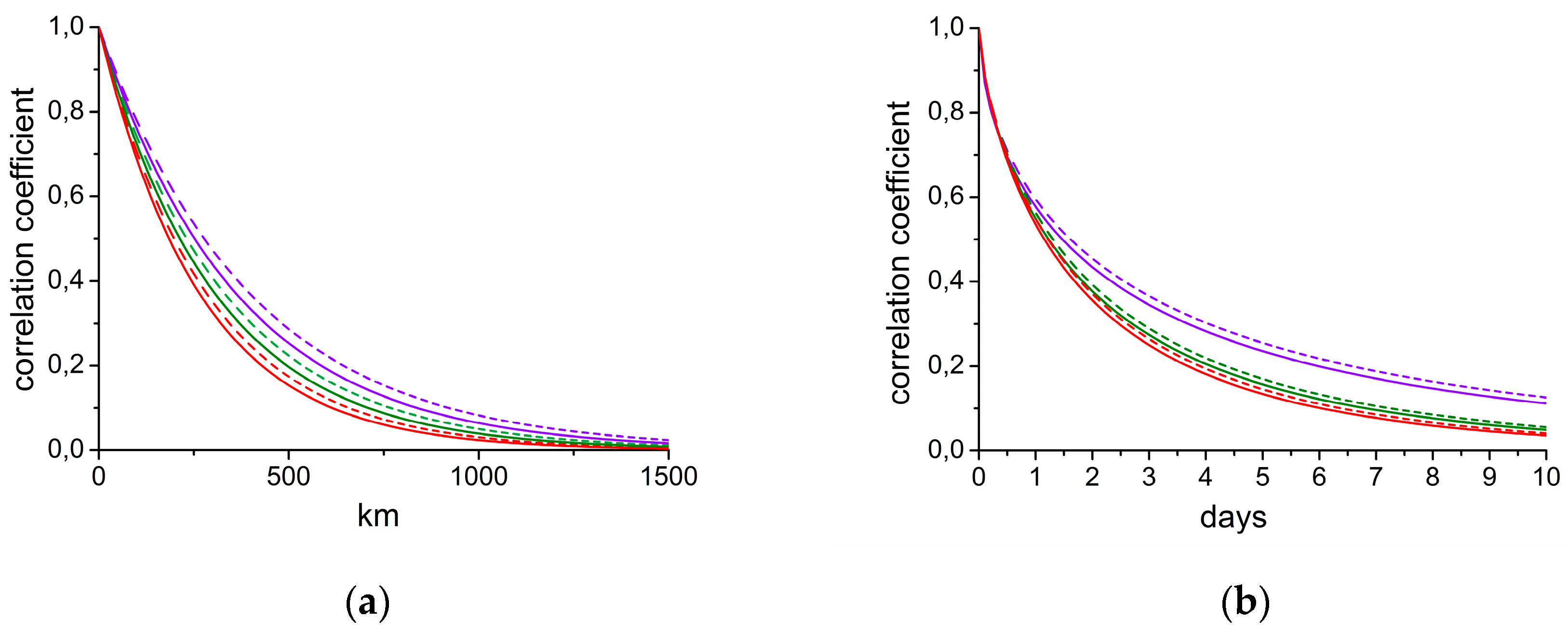
Table 1.
Root-mean-square errors (RMSE) of the aerosol optical depth (AOD) calculated using GEOS-Chem and assimilated using spatial-temporal optimal interpolation (STOI) with GEOS-Chem output as background (the reduction in RMSE of the estimate after STOI is shown in parentheses).
Table 1.
Root-mean-square errors (RMSE) of the aerosol optical depth (AOD) calculated using GEOS-Chem and assimilated using spatial-temporal optimal interpolation (STOI) with GEOS-Chem output as background (the reduction in RMSE of the estimate after STOI is shown in parentheses).
| Wavelength nm |
Granada | Lille | Minsk | |||
|---|---|---|---|---|---|---|
| GEOS-Chem | STOI | GEOS-Chem | STOI | GEOS-Chem | STOI | |
| 440 | 0.142 | 0.064 (55%) | 0.116 | 0.094 (19%) | 0.130 | 0.103 (21%) |
| 675 | 0.128 | 0.048 (62%) | 0.089 | 0.077 (14%) | 0.074 | 0.070 (7%) |
| 870 | 0.125 | 0.046 (63%) | 0.081 | 0.070 (13%) | 0.055 | 0.059 (-7%) |
Table 2.
RMSE of AOD calculated using GEOS-Chem and assimilated using STOI with climatology as background (the reduction in RMSE of the estimate after STOI is shown in parentheses).
Table 2.
RMSE of AOD calculated using GEOS-Chem and assimilated using STOI with climatology as background (the reduction in RMSE of the estimate after STOI is shown in parentheses).
| Wavelength nm |
Granada | Lille | Minsk | |||
|---|---|---|---|---|---|---|
| GEOS-Chem | STOI | GEOS-Chem | STOI | GEOS-Chem | STOI | |
| 440 | 0.142 | 0.064 (55%) | 0.116 | 0.101 (13%) | 0.130 | 0.128 (1%) |
| 675 | 0.128 | 0.048 (63%) | 0.089 | 0.079 (10%) | 0.074 | 0.069 (8%) |
| 870 | 0.125 | 0.045 (64%) | 0.081 | 0.071 (12%) | 0.055 | 0.047 (14%) |
Table 3.
RMSE of AOD calculated using GEOS-Chem and assimilated using STOI with both GEOS-Chem output and climatology as backgrounds (the reduction in RMSE of the estimate after STOI is shown in parentheses).
Table 3.
RMSE of AOD calculated using GEOS-Chem and assimilated using STOI with both GEOS-Chem output and climatology as backgrounds (the reduction in RMSE of the estimate after STOI is shown in parentheses).
| Wavelength nm |
Granada | Lille | Minsk | |||
|---|---|---|---|---|---|---|
| GEOS-Chem | STOI | GEOS-Chem | STOI | GEOS-Chem | STOI | |
| 440 | 0.142 | 0.063 (56%) | 0.116 | 0.095 (18%) | 0.130 | 0.103 (20%) |
| 675 | 0.128 | 0.047 (63%) | 0.089 | 0.077 (14%) | 0.074 | 0.060 (20%) |
| 870 | 0.125 | 0.045 (64%) | 0.081 | 0.070 (13%) | 0.055 | 0.044 (19%) |
Disclaimer/Publisher’s Note: The statements, opinions and data contained in all publications are solely those of the individual author(s) and contributor(s) and not of MDPI and/or the editor(s). MDPI and/or the editor(s) disclaim responsibility for any injury to people or property resulting from any ideas, methods, instructions or products referred to in the content. |
© 2025 by the authors. Licensee MDPI, Basel, Switzerland. This article is an open access article distributed under the terms and conditions of the Creative Commons Attribution (CC BY) license (http://creativecommons.org/licenses/by/4.0/).
Copyright: This open access article is published under a Creative Commons CC BY 4.0 license, which permit the free download, distribution, and reuse, provided that the author and preprint are cited in any reuse.


