
Submitted:
26 August 2025
Posted:
27 August 2025
You are already at the latest version
Abstract
Satellite observations can be successfully used to increase the spatial and temporal resolution of ground-based data. Recently, many studies exploited satellite observations to estimate the Particulate Matter (PM) mass concentration near the ground from Aerosol Optical Depth (AOD) data. This is a promising field of research, which can expand the coverage of local and regional ground-based networks. However, significant gaps remain in the correct representation of local aerosol properties such as the Effective Radius, and of the aerosol growth due to high humidity conditions (i.e., hygroscopic growth). Standard PM measurements are taken at dry conditions, thus needing a corrective function to successfully correlate with satellite AOD.
This study exploits ground-based measurements taken at ambient conditions by an Optical Particle Counter (OPC) in the city of Bologna, in the Po Valley. In this way, the need for corrective functions is overcome. The OPC used in this study, the LOAC (Light Optical Aerosol Counter), measures Particle Number concentration and provides information on particle typology, which are used to compute the Effective Radius and the PM at ambient Relative Humidity (RH). A linear regression between AOD and PM is performed by exploiting the theoretical relationship which depends on the local aerosol characteristics estimated from the available LOAC data.
Results show that using all the auxiliary data (instead of the PM alone) improves the linear regression parameters: as an example, the Pearson's correlation coefficient increases from 0.55 to 0.76. The increase is independent on the season. The linear function between AOD and PM has a slope of 0.81 or 1.04 depending on the estimate of the Effective Radius considered.
Keywords:
satellite remote sensing
; aerosol optical depth
; particulate matter
; air quality monitoring
1. Introduction
Health effects of aerosol pollution are well documented in literature [1,2], with effects ranging from allergies to chronic respiratory diseases and even carcinogenic effects as stated by WHO in 2013 [2]. For this reason, the continuous monitoring of aerosol concentrations within urban areas and in background and remote locations is of primary importance for studies focused on exposure and risk assessment practices.
Aerosol monitoring is usually performed with conventional and standardized procedures that employ daily in-situ measurements of Particulate Matter mass concentration (PM, in ) at fixed stations. According to Martin et al. [2], in Europe there are 3 to 4 PM monitors per million of inhabitants, while in other continents the situation is even worse. As a result, most surface areas are underrepresented in terms of spatial and temporal characterization of PM.
In the last decades, the scientific community has pursued the idea of using satellite observations to increase the time and space resolutions of the sparse ground-based network [2]. It has been demonstrated that the satellite Aerosol Optical Depth (AOD) can be correlated to the ground-based PM by an empirical relation that considers meteorological variables such as the Relative Humidity (RH) and the Planetary Boundary Layer Height (PBLH). This relation can be approximated as being linear in particular cases such as in urban areas, where the aerosols are well-mixed inside the PBL and in absence of thick aerosol layers at higher altitudes [2,2]. For example, Wang et al. [2] found a correlation coefficient equal to 0.7 (out of 1) between MODIS AOD and hourly PM2.5; the correlation increased to values higher than 0.9 when lowering the time resolution to monthly averages. Koelemeijer et al. [2] considered several European cities and found a linear correlation coefficient of 0.6 between MODIS AOD and daily PM2.5, over rural and background urban stations.
More complex methodologies employ data-driven models (statistical or Machine Learning) or chemistry transport models [2]. Each methodology has its strengths and weaknesses. For example, data-driven models require huge datasets for the training phase, and it is complex to select the most significant variables to being included. On the other hand, the use of chemical transport models requires a heavy computational power, and their accuracy depends on the quality of input data such as emission sources, land use, meteorology, etc. Lastly, there are also semi-empirical methodologies, which employ measurements at selected locations to estimate the coefficients of the linear function that relates AOD and PM. This type of methodology presents low computational costs and is based on physical relationships, but the input data may be spatially and temporally sparse [9]. Nonetheless, a semi-empirical method can be implemented with some caution and tailored to the case study, depending on the available data. Ferrero et al. [10] considered factors such as the spatial representativeness of the ground-based PM with respect to the satellite footprint and the temporal difference between the satellite overpass time and the daily or hourly PM measurements, as well as the vertical characteristics of the atmosphere.
In the revised Ambient Air Quality Directive from the European Commission [11], the annual limit for has been lowered to 10 , while the 24-hour average limit is 25 , to be exceeded less than 18 times during the year. The Po Valley, in Northern Italy, is an area known for frequent exceedances of air pollution limit values, including those for aerosol pollution. This is due to its high urbanization and industrialization density, and is exacerbated especially in the winter period by its peculiar geography bounded by the Alps and the Apennines mountains limiting atmospheric circulation, as well as characteristic weather patterns characterized by stability conditions that often trap and accumulate pollutants for long periods.
In the last decades, MODIS AOD has been used with empirical, statistical and machine learning methodologies to estimate the PM spatial variability in the area. Koelemeijer et al. [2] and Di Antonio et al. [12] managed to highlight the contrast between the high atmospheric pollution in the Po Valley compared to nearby areas. Di Nicolantonio et al. [13] was one of the first studies to implement a semi-empirical methodology, and found a correlation of 0.68 and 0.59 between MODIS AOD and daily PM2.5, reaching values of 0.7 when using monthly averages. More recent studies [10,14,15] exploited MAIAC AOD product [16], retrieved by MODIS observations with a spatial resolution of 1 km x 1 km, to better characterize the spatial variation of PM.
Among recent studies in the area, Ferrero et al. [10] and Arvani et al. [14] considered the use of a hygroscopic growth function within their methodologies and found that the results of linear correlation between AOD and PM were not significantly improved. Hygroscopicity is the property of some aerosols to grow in size according to their water uptake, changing their optical properties as well as their mass concentration. A corrective function is needed when relating the AOD, which is retrieved at ambient humidity, and the PM, which is measured in controlled environments with RH < 50%. The use of this function should improve the correlation between the two quantities. The main issue is the empirical nature of this function, whose coefficients depend on the local aerosol characteristics [17,18].
In recent years, Optical Particle Counters (OPCs) have been employed as part of air quality monitoring networks because of their portability, higher temporal resolution and limited costs with respect to conventional reference instrumentation utilized for PM measurement [19]. OPCs detect the Particle Number concentration (PN) in specific size bins and retrieve the PM mass concentration through an internal algorithm. If the OPC is operated at ambient conditions, it estimates the ambient or “wet” PM, which is supposedly better correlated with AOD than the “dry” PM from standard measurements. In fact, the hygroscopic function is not needed when relating “wet” PM with AOD at ambient conditions. OPC data has also been used as auxiliary data in previous studies such as [10], but to our knowledge, no previous study directly relates OPC-derived PM to satellite AOD.
The present study compares estimates of PM retrieved by a specific Optical Particle Counter, the LOAC (Light Optical Aerosol Counter) operated at ambient conditions, with MAIAC AOD for the year 2023 over the city of Bologna, in the Po Valley. The study also attempts to find a semi-empirical linear function to relate the "wet" PM2.5 and the satellite AOD, with the use of auxiliary data.
PN measurements from the LOAC are used as an estimate of the aerosol Particle Size Distribution (PSD), allowing the computation of the Effective Radius of the aerosol mixture. The Effective Radius is an important variable in the correlation between the optical properties and the mass concentration of aerosols and strongly affects the radiative properties derived from satellite. In addition, the LOAC infers information concerning the aerosol type (such as Salt, Mineral, and Carbonaceous aerosols) [20] which is used in the semi-empirical methodology together with Effective Radius and PBLH.
2. Materials and Methods
2.1. Study Area
In this work, ground-based observations of meteorological variables and aerosols physical characteristics were obtained during an intensive experimental field campaign conducted in 2023 in the urban area of Bologna, Italy, located in the Southern border of the Po Valley.
The Po Valley is characterized by a distinct seasonality of aerosol mass concentration. During winter, the frequent stability conditions and low wind velocity tend to favour the trapping and accumulation of pollutants [21]. Particle accumulation give rise to a concentration gradient at the PBL level, which correlates with a vertical gradient of Relative Humidity [22]. The concentration gradient is also linked to a vertical gradient of aerosol extinction. During winter, aerosol extinction tends to increase in the lowest levels of the atmosphere and concurrently to decrease at altitudes higher than 1 km; during spring and summer, the extinction is evenly distributed in the atmospheric column. As a result, during winter more than 80% of AOD refers to particles below 1 km [23].
The relative composition of PM also varies during the year according to changes in aerosol emissions. The 75% of urban PM2.5 in the Po Valley is composed of water-soluble inorganic compounds (Nitrates and Sulphates) and Carbon [24]. Local emission sources in cities comprise different types of fuel due to traffic and residential heating, which leads to different fractions of Black Carbon and organic compounds during the year [25]. In the city of Bologna, at least 40% of PM2.5 is due to traffic emissions, 24% is composed of road dust, and 8% is due to biomass burning; the levels of mineral dust, which are usually negligible, often increase in the summer during episodes of desert dust intrusion [26]. A change in the composition of the aerosol mixture affects the average optical properties retrieved from remote sensing observations, such as satellite AOD. For this reason, when comparing the aerosol mass concentration and the total extinction, it is important to obtain information about the chemical composition or the optical behaviour of the aerosol mixture.
2.2. Methodology
Based on theoretical considerations, a linear correlation between aerosol extinction and PM2.5 can be established (e.g., [2]). Formally:
Equation 1 links the aerosol extinction coefficient at ground level with the corresponding mass concentration . Usually, the mean extinction coefficient and the mean extinction efficiency are computed at visible wavelengths. All the variables are referred to ambient conditions. is the aerosol average mass density and is the Effective Radius of the aerosols. The Effective Radius of the PSD is defined as:
and the average Extinction Efficiency is defined as:
The total AOD is computed as the integral of the aerosol extinction coefficient along the atmospheric column. In the assumption that all aerosols in the atmospheric column are well-mixed and placed below the PBL height, the vertical profile can be approximated as:
so that an approximate formula relating PM2.5 to AOD (at ambient conditions) is available:
where we underline the fact that PM is at ambient RH. The term represents the ratio between the mass concentration and the extinction coefficient of the aerosols. Note that all variables that define the term A can be derived from OPC measurements and are therefore consistent with the measurement of .
A linear regression can be performed by applying the function:
with and . Theoretically, the slope values will vary throughout the year according to the varying aerosol mixtures and the meteorological conditions impacting on the location of interest. It has been verified that, in general, the higher the PBLH, for example during summer, the lower the linear correlation (e.g. [27]). When using Eq. 6 to derive the empirical coefficient, the slope is considered to be constant in the time window and location considered by the dataset. Lastly, b is the offset between and and, in theory, it will not vary seasonally.
The present study also analyses the linear regression between PM2.5 and the AOD corrected by all available auxiliary data: Effective Radius, average mass density and average optical properties, thus having an estimate of the term A. The linear correlation is performed with Eq. 6 and with and alternatively with and and the results are compared.
PM2.5 absolute uncertainty is fixed as the standard deviation and AOD relative uncertainty is 0.05 (see Sec. 2.4). Uncertainties for and are computed with the relative uncertainty rule:
2.3. OPC Data
OPC measurements were obtained by a LOAC (Light Optical Aerosol Counter) [20] mounted on the rooftop of the Department of Physics and Astronomy (DIFA) of the University of Bologna (lat: 44.499, lon: 11.354), at about 22 m from the ground (from now on named only DIFA). The surrounding area is a vegetated street inside the historical centre of Bologna (Figure 1). The LOAC dataset covers the months from February to September 2023. The LOAC retrieves the Particle Number (PN) concentration () in 19 size bins for particle diameters between 0.2 and 30 (Table 1) by the use of laser beams at 650 nm wavelength. By using two scattering angles (12° and 60°) it also determines the degree of absorption by the detected particle, from transparent to highly absorbing. This estimate is used to classify the particles, divided in five size classes (Table 2), in four types: “droplet”, “salt”, “mineral”, “carbon”. From the PN measurements and the particle type, the PM1, PM2.5, and PM10 () are calculated with an internal algorithm which uses a suitable value of particle mass density () according to particle type. In general, all OPC instruments are highly affected by high Relative Humidity, cloudy conditions and precipitation events (eg. [28]). As such, recent studies recommend to perform measurements with such sensors under low time resolutions (hourly and daily averages) and clean sky conditions [29].
The 1-minute PN and PM2.5 data is screened with a Hampel filter on a 10-minute window [30] to remove outliers and then averaged hourly. The Effective Radius is also computed by discretizing Eq. 2, which becomes:
where is the Particle Number concentration in the size bin i and is half the nominal diameter of size bin i. This is because the Particle Number concentration in size bin i is the total value of within the size bin: . The is computed with the original filtered 1-minute PN data and then averaged hourly.
The particle type dataset from LOAC is used together with PN data to compute the average aerosol Extinction Efficiency and mass density. This is done by computing
- the Number Ratio (NR) of each particle type in each size bin,
- the average single particle Extinction Efficiency of each particle type in each size bin
and by choosing the proper mass density for each particle type, assuming it is the same in all size bins. In Renard et al. 2016 [20] it is advised to use particle type information with a statistical approach. For each hour, we consider the number of occurrences of each particle type in each size bin, divide it by the total number of observations in each size bin in that hour (maximum of 60), and convert the fraction into decimal percentage. In this way, we define the Number Ratio in size bin i for the particle type x.
In Renard et al. 2010 [31], the absorption of different particle types is defined in relation to different values of the imaginary part k of the Refractive Index (RI). The “salt” and “mineral” particle type match simulations of optical properties for glass beads with , while the “carbon” particle type match simulations with , considered at the laser wavelength of 650 nm. We consider the optical properties of aerosols as defined in the database OPAC [32]. The urban aerosols are defined as a mixture of Soluble and Insoluble aerosols, characterised by low absorption at 650 nm ( and ) and of Black Carbon (or Soot) which has a high absorption at 650 nm (). In this study, we assume that each LOAC particle type can be related to each OPAC aerosol type:
- “salt” LOAC type related to “Soluble” OPAC type (here considered at RH = 50%),
- “mineral” LOAC type related to “Insoluble” OPAC type,
- “carbon” LOAC type related to “Soot” OPAC type,
and use the related single particle Extinction Efficiency values.
varies with particle radius r in different ways for each particle. We compute as the average value of in the size bin i for type x. Lastly, the average Extinction Efficiency for each LOAC observation is discretized from Eq. 3 as:
while the average mass density is computed as:
where are the nominal values of mass density for each LOAC particle type x (same value for all size bins). We choose to use the same mass density values used in the computation of the PM instead of the mass density values reported in OPAC for the chosen aerosol types.
2.4. AOD
MAIAC AOD is retrieved at 550 nm from MODIS observations at high spatial resolution (1 km x 1 km) on a fixed grid. It has a better performance over bright surfaces compared to other algorithms and has been previously applied over urban areas [33]. In cases of anthropogenic aerosols, AOD below 0.12 can be overestimated. AOD uncertainty indicated in the product files is related to surface brightness. A value below 0.05 allows the algorithm to perform a standard retrieval [33,34]. A 5% uncertainty value for the single retrieval values can be used. More information on the retrieval can be found at [16]. Intense pollution cases in urban areas within the Po Valley, especially in very high polluted cities such as Milan and Turin, can be sometimes interpreted as clouds and filtered out [14].
Co-location of AOD and ground-based data at DIFA site is performed on the fixed grid used in MAIAC retrievals. The cell containing the DIFA location is selected (Figure 1). This grid cell refers to the innermost part of Bologna historical centre, characterised by medium-bright surfaces, traffic and low industrial emissions. The AOD data is acquired for the whole period covered by the LOAC dataset (February-September 2023). The total number of satellite overpasses in the study period is 985, but only 26.8% is characterized by a successful AOD retrieval. The available retrievals are few during April and May (15-16%) and more frequent in August (41%).
Considering the dataset of co-located AOD retrievals, AOD uncertainty due to surface brightness is lower than 0.045 with a median of 0.016, and AOD values are lower than 0.45 with a median of 0.14. This means that the retrievals used in the following analysis are computed with the standard algorithm, and likely not affected by underestimation.
2.5. Auxiliary Variables
Planetary Boundary Layer Height (PBLH) is retrieved by a ceilometer Vaisala CL31, mounted on the rooftop of DIFA alongside the LOAC. The ceilometer continuously measures the vertical backscatter signal from the ground level to a maximum of 7.5 km and provides estimates of PBLH with a temporal resolution of 16 s and a vertical resolution of 10 m. It also provides an estimate of Cloud Height if clouds are detected. The internal algorithm is based on the difference in backscatter signal between the mixing layer, where the signal is higher due to aerosols, and the free atmosphere, where the backscatter signal abruptly drops to very small values in absence of scattering layers [35]. An incorrect PBLH detection can be related to the presence of residual layers or to PBL changes during the early evening. In these cases, the ceilometer detects more than one PBLH value, with the highest one usually corresponding to residual layers or incorrectly detected clouds [36].
The original dataset is averaged on a 10 minutes time frame around the satellite overpass and the PBLH is selected from the retrieved Boundary Layer heights. Three possible PBLH values are retrieved by the Ceilometer algorithm. The lowest value usually refers to the strong gradient between the ground-level atmospheric pollution and the aerosols mixed above, or to a consistent residual layer (especially in winter), with values below 600 m. The middle layer, when present, is the most probable PBLH value if below 1.5 km, otherwise it may refer to clouds during precipitation or cloudy days. The third layer usually refers to clouds or extinction gradients due to complex vertical profiles. In this work, we choose the first PBLH value if higher than 600 m and the second one if below 2 km. This is consistent with the average PBLH values in the area (as mentioned for example in [23]).
Auxiliary data include quality-proofed data from the local environmental agency (ARPAE) [37]: 30-minute Relative Humidity and hourly Precipitation Rate are measured from the closest meteorological station, Bologna Idrografico (lat: 44.499, lon: 11.346), located 620 m from DIFA; daily "dry" PM2.5 from ARPAE Porta San Felice station (lat: 44.499, lon: 11.328), located 2120 m from DIFA. In Figure 1 the stations are shown alongside DIFA and the AOD cell from satellite.
3. Results
3.1. Analysis of the Particle Concentration Variability
In the following, we analyze the data obtained by the LOAC. The measurement period considered in this work (February-September 2023) was characterized by a particular variability in the meteorological conditions impacting on the study area.
The month of May 2023 was affected by three exceptional rainfall events (May 2, 16, and 17), with cumulative daily rainfall values higher than 100 mm recorded at the Bologna Idrografico station. Other minor rainfall events occurred throughout the measurement period. Figure 2 shows daily averages of “wet” PM2.5 from LOAC and RH from Bologna Idrografico for the whole period. Precipitation events with rainfall higher than 20 mm are highlighted in grey. As noted in [29], LOAC measurements are affected by the hygroscopic growth of particles under precipitation events and high RH conditions. This is apparent from the daily values of PM2.5 recorded during the study period, which are all below 35 except for observation records during precipitation events, in which PM2.5 reaches values above 50 .
Desert dust intrusions were frequent during the months of June and July. The monthly PSD averages in Figure 3 shows a corresponding increase in particles with radius greater than , compared to particles with smaller radii, during these months. PSD is computed by dividing the PN by the width of each size bin, as explained in Section 2. The Effective Radius, computed with Eq. 8, shows values larger than during precipitation events in May 2 and 16, and higher than between June , and July and . Data from AERONET nearest stations of Modena and San Pietro Capofiume highlight that, during that time, the Angstrom Exponent was below 0.5 in June and below 0.6 in July. Low values of are associated with desert dust transport which is frequent in Italy during summer, with dust plumes that also reach the Po Valley and Bologna [40]. Except for precipitation and dust transport events, the Effective Radius is less than during the measurement period.
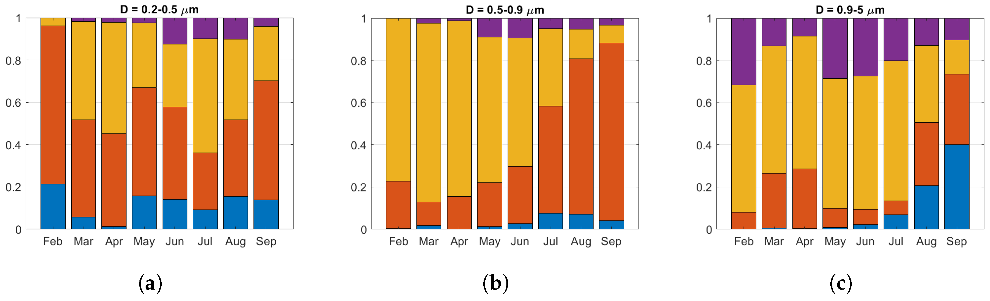
Figure 5 shows the monthly particle type occurrences, described by the Number Ratios as defined in Section 2. Only the first three size ranges are shown, consisting of particles with diameters between and (as specified in Table 2). Particles in the fourth size range () consist of water droplets or unidentified types. Particle types in the two largest size ranges () are mostly not identified, probably due to measured PN concentrations lower than . The “salt” and “mineral” types are present in the first two size ranges in varying proportions during the year. In the third size range (), “mineral” type is the most common, but also the “carbon” type is consistently present.
When calculating and , water droplets are not considered, while the values for larger size bins are set to constant values due to the high frequency of unidentified particle types.
Figure 4.
Daily Effective Radius from LOAC (blue line). Grey areas refer to days with total precipitation greater than 20 mm. Red areas refer to dust transport events.
Figure 4.
Daily Effective Radius from LOAC (blue line). Grey areas refer to days with total precipitation greater than 20 mm. Red areas refer to dust transport events.
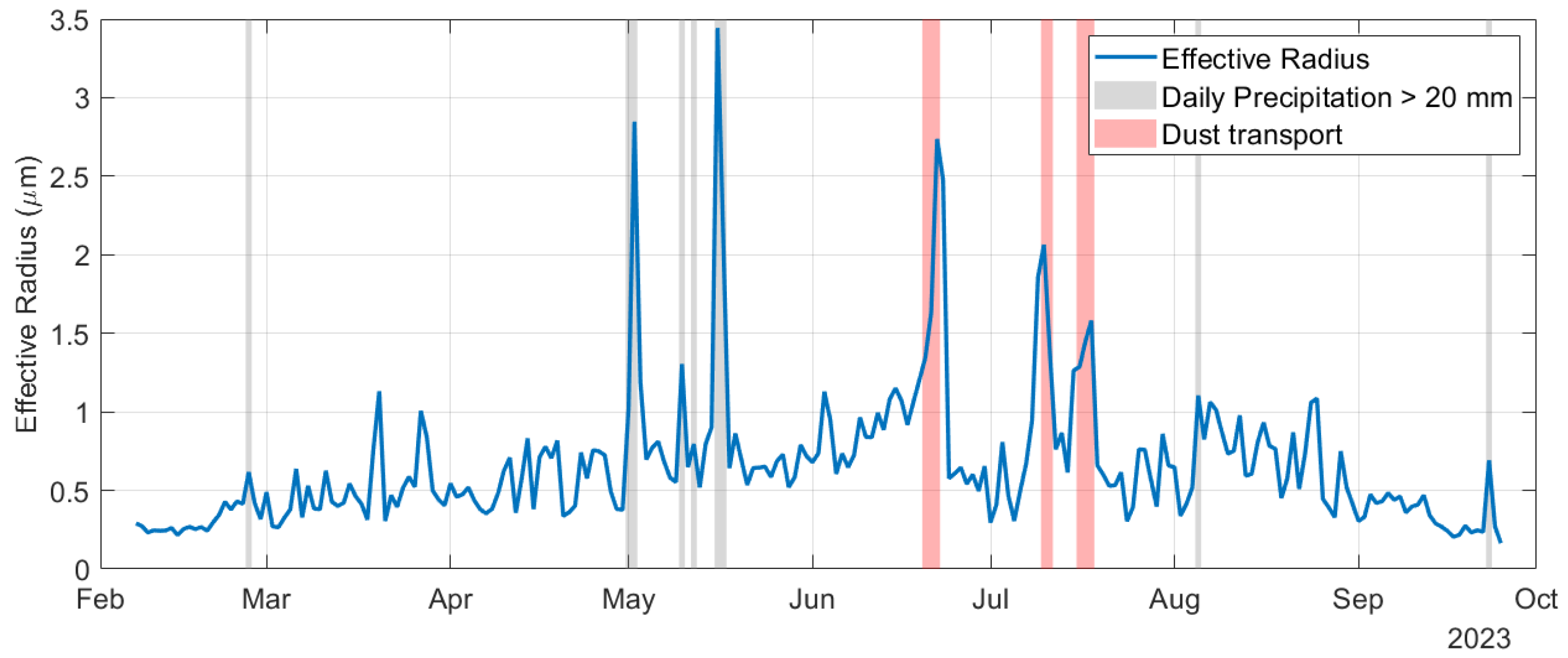
Figure 5.
Monthly Number Ratio of the detected particle types in the first 3 size classes. Blue = droplet, Red = salt, Yellow = mineral, Purple = carbon. (a) Size class . (b) Size class . (c) Size class .
Figure 5.
Monthly Number Ratio of the detected particle types in the first 3 size classes. Blue = droplet, Red = salt, Yellow = mineral, Purple = carbon. (a) Size class . (b) Size class . (c) Size class .
3.2. Methodology Application
The present section explains the assumptions and the results of the linear regressions. The goodness of the correlation is evaluated using the Pearson’s correlation coefficient R (95% confidence) and the linear regression performance is measured by the coefficient of determination and Root-Mean Square Error (RMSE). The linear regression function and the correlated variables are defined in Eq. 6. We also normalize the coefficient A considering the different units of measurement between PM2.5 (), (), () and (); by definition, is unitless.
The uncertainty associated with the hourly averages of and is the standard deviation. During particular events such as precipitation and dust transport, the uncertainties are higher because of the higher variability in the PN measurements. For periods when the AOD data is available, the relative uncertainty of is below 40% with an average of 36% and the relative uncertainty of is lower than 30% with an average of 22%. Only this data is considered in the methodology because the AOD is needed to perform the linear regressions.
On the other hand, AOD has a nominal relative uncertainty of 5% and the composed uncertainty of is between 5% and 10% in the whole AOD-PBLH dataset. The uncertainty for is between 5% and 50%, which can be higher than the uncertainty on Y. This is expected as it is a composed uncertainty computed from X and .
First, we perform the linear regression with and , without adding auxiliary information. We consider PM2.5 data whose standard deviation is less than and whose relative uncertainty is less than 20%. We also consider AOD data between 0.01 and 0.35 to avoid errors in the retrieval algorithm. PBLH values under 600 m are considered faulty retrievals and set to 800 m. By using these rules, May and September data are filtered out, as well as several data points during June and July. The final dataset therefore consists of a total of 56 observations available.
The Pearson’s correlation coefficient R is 0.5587 (out of 1), indicating a weak linear correlation between the two variables. The linear regression function has and , which is not enough for a good linear fit. The linear function is . The linear function is shown in Figure 6a with the selected data points. As expected, the relationship between the variables does not show any clear dependence on RH, suggersting that there is no need for a hygroscopic correction factor.
For comparison, we perform the linear regression using daily "dry" PM2.5 from reference ARPAE station Porta San Felice in the same temporal window. As PM2.5 data is obtained from reference instruments, we assume that the uncertainty is always below 20%. We assume that the PBLH does not change significantly between the station and DIFA, therefore using PBLH obtained from the ceilometer. The selected AOD refers to the cell whose centre is closest to the ground-based station. To obtain daily averages of , we first compute the fraction and then average daily the available data. In this case, the regression is performed on 102 data points between February and September 2023. The value of R is 0.1558, indicating an absence of linear correlation. As it is apparent from Figure 6b, "dry" PM2.5 and the corrected AOD seem uncorrelated, and there is no correlation with the respective RH value (daily averaged). The linear function is with and .
Now we consider LOAC PM2.5 and the auxiliary information to compute and its uncertainty. We recall that is the theoretical coefficient between "wet" PM2.5 and . We filter data whose uncertainty is higher than . The filtered subset comprises 49 data points between February and July. The Pearson’s correlation coefficient is 0.7610, indicating a much higher linear agreement between the variables. The linear regression function has and , which indicates a slightly better linear fit compared to results from previous studies such as [13,41]. The linear function, presented in Figure 7a, is .
The offsets b in both linear functions are compatible with each other within confidence bounds (see also Table 3). This means that this value depends on other factors, such as the difference between the point measurements (LOAC and ceilometer data) and the satellite AOD retrieval (with a footprint of ). Theoretically, the slope of the second linear function should be close to 1, as A represents the theoretical slope that relates PM2.5 to AOD and should account for all the variability. The value of 0.812 can be interpreted as the effects of the assumptions made for the methodology application.
It should be noted that the smallest particle diameter detected by the LOAC is (Table 1). This excludes the detection of particles with radii less than , that are almost negligible in the computation of mass concentration, but can have a significant contribution in terms of particle number concentration and in the extinction of radiation. Moreover, the Effective Radius should be calculated considering particles with radii starting from , for example, as in the definition of aerosol types in OPAC [32]. The same is valid for the computation of and .
To improve the calculation of these parameters, we add a smaller size bin for diameters , whose Number Ratio for each particle type is assumed to be the same as the first size range () and whose Particle Number concentration is extrapolated by considering PN values in size bins 1 to 5. Taking into account only the 49 data points used for the second linear regression, values fall in the range of the original , values are of the original , and values are nearly equal to the original ones. We repeat the linear regression with the new values of , computing . In this case, the slope of the linear function reaches a value of with , and (shown in Figure 7b). To complete the analysis, we also compute . In this case the linear regression has a slope with , and . Finally, when using the new values for both variables, we compute and in this case the slope is , with , and . Table 3 summarizes the linear correlation results obtained in each case considered so far. The fit results improve when using the new computed values of while they do not improve when considering also the new computed values of .
4. Discussion
We show that the use of ’wet’ PM2.5 mass concentration observations is correlated to the collocated satellite AOD, thus avoiding the application of hygroscopic corrections to the ground-based data. The Pearson’s correlation coefficient shows that the "wet" hourly PM2.5 is linearly correlated to AOD, even without using auxiliary information with the exception of the PBL values which is always considerd. For comparison, "dry" PM2.5 from reference ground-based measurements only yields a coefficient , indicating the absence of a linear correlation with satellite AOD.
The "wet" PM2.5 is representative of the mass concentration of the particulate matter in humidity conditions, consistent with the AOD satellite measurement. The analysed data show that higher values of both PM and AOD are generally associated to higher values of RH, contrary to "dry" PM2.5 which is measured at fixed RH values lower than 50%. This allows us to use data from all year instead of selecting data by season, as the main seasonal differences depend on RH, as well as other meteorological variables such as Atmospheric Temperature and Wind Speed. This is an element of novelty with respect to previous works on the same topic, while reaching results comparable to previous studies [2,10,13,14].
Moreover, a Pearson’s correlation coefficient of is obtained when AOD is AOD is multiplied by parameters obtained by the LOAC. An increase in R points at a better linear correlation between the variables. The coefficient of determination of agrees with previous studies that used a linear fit for the correlation [13,41], with the addition that in our case the linear function is valid for the entire temporal window investigated (February-September 2023), without the need of using different coefficients depending on the specific season or the month.
The slope of the linear function between "wet" PM2.5 and adjusted AOD is 0.82, which is lower than the perfect fit value of 1. This means that the applied corrections do not fully relate the two variables linearly. This is an expected conclusion due to the high relative uncertainty of the computed values of the theoretical slope , which in turn is due to the high relative uncertainty of with respect to PM2.5, and to the absence of a quantitative estimate for the uncertainty of the particle type inferred from the LOAC measurements. Moreover, the linear approximation may not hold for all possible cases.
By repeating the linear regression with an alternative calculation of , the slope of the linear function reaches a value of 1.04 while maintaining a comparable goodness of fit (), relative error on coefficients (), and Pearson’s coefficient (). The alternative is calculated by extrapolating Particle Number concentration for smaller particles, which are not measured by the LOAC, but are not negligible in the computation of aerosol optical properties. The new values are lower than the original ones while maintaining comparable uncertainties. This suggests that using PN measurements from LOAC may overestimate the value of in urban environments.
Our methodology takes into account the theoretical relationship between PM mass concentration and total aerosol extinction, and is able to correlate them with a slope close to 1. Similarly to previous studies, an offset is needed in the linear correlation to account for factors other than aerosol properties and meteorology (e.g., local traffic).
An appropriate correction is also needed to compare the "wet" PM2.5 retrieved from satellite data with standard measurements of “dry” PM2.5. It should consist of an empirical function whose coefficients are related and fine-tuned in accordance with the aerosols features of the considered location. We argue that the conversion from "wet" to "dry" PM2.5 is secondary to the estimation of PM from satellite data and therefore it is not furtherly studied in the present work.
Author Contributions
Conceptualization, G.P.P. and T.M.; formal analysis, G.P.P.; data curation, G.P.P. and A.F.; writing—original draft preparation, G.P.P.; writing—review and editing, T.M. and E.B.; supervision, T.M. and E.B.. All authors have read and agreed to the published version of the manuscript.
Funding
This research was funded by the EU - NextGenerationEU with funds made available by the National Recovery and Resilience Plan (NRRP) Mission 4, Component 1, Investment 4.1 (MD 351/2022) – NRRP Research.
Data Availability Statement
The MAIAC dataset, MCD19A2 MODIS/Terra+Aqua Aerosol Optical Thickness Daily L2G Global 1km SIN Grid, was acquired from the Level-1 & Atmosphere Archive and Distribution System (LAADS) Distributed Active Archive Center (DAAC), located in the GoddardSpace Flight Center in Greenbelt, Maryland (https://ladsweb.modaps.eosdis.nasa.gov/) and is accessible at https://doi.org/10.5067/MODIS/MCD19A2.006 [16]. The AERONET data is available at https://aeronet.gsfc.nasa.gov/ [38]. PM2.5 and meteorological data from ARPAE are accessible at https://dati.arpae.it/ [37]. Ceilometer data and LOAC data available on request from the authors.
Acknowledgments
We graciously thank our colleagues Silvana di Sabatino and Francesco Barbano for the availability and curation of the Ceilometer data. The study was partly developed within the RETURN “Multi-risk science for resilient communities under a changing climate” (National Recovery and Resilience Plan – NRPP, Mission 4, Component 2, Investment 1.3 – D.D. n.341 15/3/2022, PE0000005).
Conflicts of Interest
The authors declare no conflicts of interest. The funders had no role in the design of the study; in the collection, analyses, or interpretation of data; in the writing of the manuscript; or in the decision to publish the results.
References
- Sharma, S.; Chandra, M.; Kota, S.H. Health effects associated with PM2.5: A systematic review. Curr. Pollut. Rep. 2020, 6, 345–367. [Google Scholar] [CrossRef]
- Thangavel, P.; Park, D.; Lee, Y.C. Recent insights into particulate matter (PM2.5)-mediated toxicity in humans: An overview. Int. J. Environ. Res. Public Health 2022, 19, 7511. [Google Scholar] [CrossRef] [PubMed]
- Organization, W.H. World health statistics 2013; World Health Organization, 2013.
- Martin, R.V.; Brauer, M.; van Donkelaar, A.; Shaddick, G.; Narain, U.; Dey, S. No one knows which city has the highest concentration of fine particulate matter. Atmospheric Environment: X 2019, 3, 100040. [Google Scholar] [CrossRef]
- Hoff, R.M.; Christopher, S.A. Remote Sensing of Particulate Pollution from Space: Have We Reached the Promised Land? Journal of the Air & Waste Management Association 2009, 59, 645–675. [Google Scholar] [CrossRef] [PubMed]
- Wang, J.; Christopher, S.A. Intercomparison between satellite-derived aerosol optical thickness and PM2.5 mass: Implications for air quality studies. Geophysical Research Letters 2003, 30. [Google Scholar] [CrossRef]
- Koelemeijer, R.; Homan, C.; Matthijsen, J. Comparison of spatial and temporal variations of aerosol optical thickness and particulate matter over Europe. Atmospheric Environment 2006, 40, 5304–5315. [Google Scholar] [CrossRef]
- Ma, Z.; Dey, S.; Christopher, S.; Liu, R.; Bi, J.; Balyan, P.; Liu, Y. A review of statistical methods used for developing large-scale and long-term PM2.5 models from satellite data. Remote Sensing of Environment 2022, 269, 112827. [Google Scholar] [CrossRef]
- Li, Y.; Yuan, S.; Fan, S.; Song, Y.; Wang, Z.; Yu, Z.; Yu, Q.; Liu, Y. Satellite remote sensing for estimating PM2.5 and its components. Curr. Pollut. Rep. 2021, 7, 72–87. [Google Scholar] [CrossRef]
- Ferrero, L.; Riccio, A.; Ferrini, B.; D’Angelo, L.; Rovelli, G.; Casati, M.; Angelini, F.; Barnaba, F.; Gobbi, G.; Cataldi, M.; et al. Satellite AOD conversion into ground PM10, PM2.5 and PM1 over the Po valley (Milan, Italy) exploiting information on aerosol vertical profiles, chemistry, hygroscopicity and meteorology. Atmospheric Pollution Research 2019, 10, 1895–1912. [Google Scholar] [CrossRef]
- Directive - EU - 2024/2881 - EN - EUR-LEX. https://eur-lex.europa.eu/legal-content/EN/TXT/?uri=OJ:L_202402881. Accessed: 2025-08-07.
- Di Antonio, L.; Di Biagio, C.; Foret, G.; Formenti, P.; Siour, G.; Doussin, J.F.; Beekmann, M. Aerosol optical depth climatology from the high-resolution MAIAC product over Europe: differences between major European cities and their surrounding environments. Atmospheric Chemistry and Physics 2023, 23, 12455–12475. [Google Scholar] [CrossRef]
- Di Nicolantonio, W.; Cacciari, A.; Tomasi, C. Particulate Matter at Surface: Northern Italy Monitoring Based on Satellite Remote Sensing, Meteorological Fields, and in-situ Samplings. IEEE Journal of Selected Topics in Applied Earth Observations and Remote Sensing 2009, 2, 284–292. [Google Scholar] [CrossRef]
- Arvani, B.; Pierce, R.B.; Lyapustin, A.I.; Wang, Y.; Ghermandi, G.; Teggi, S. Seasonal monitoring and estimation of regional aerosol distribution over Po valley, northern Italy, using a high-resolution MAIAC product. Atmospheric Environment 2016, 141, 106–121. [Google Scholar] [CrossRef]
- Stafoggia, M.; Schwartz, J.; Badaloni, C.; Bellander, T.; Alessandrini, E.; Cattani, G.; de’ Donato, F.; Gaeta, A.; Leone, G.; Lyapustin, A.; et al. Estimation of daily PM10 concentrations in Italy (2006–2012) using finely resolved satellite data, land use variables and meteorology. Environment International 2017, 99, 234–244. [Google Scholar] [CrossRef]
- Lyapustin, A.; Wang, Y.; Korkin, S.; Huang, D. MODIS Collection 6 MAIAC algorithm. Atmospheric Measurement Techniques 2018, 11, 5741–5765. [Google Scholar] [CrossRef]
- Zieger, P.; Fierz-Schmidhauser, R.; Weingartner, E.; Baltensperger, U. Effects of relative humidity on aerosol light scattering: results from different European sites. Atmospheric Chemistry and Physics 2013, 13, 10609–10631. [Google Scholar] [CrossRef]
- Hänel, G. An attempt to interpret the humidity dependencies of the aerosol extinction and scattering coefficients. Atmospheric Environment (1967) 1981, 15, 403–406. [Google Scholar] [CrossRef]
- Karagulian, F.; Barbiere, M.; Kotsev, A.; Spinelle, L.; Gerboles, M.; Lagler, F.; Redon, N.; Crunaire, S.; Borowiak, A. Review of the Performance of Low-Cost Sensors for Air Quality Monitoring. Atmosphere 2019, 10. [Google Scholar] [CrossRef]
- Renard, J.B.; Dulac, F.; Berthet, G.; Lurton, T.; Vignelles, D.; Jégou, F.; Tonnelier, T.; Jeannot, M.; Couté, B.; Akiki, R.; et al. LOAC: a small aerosol optical counter/sizer for ground-based and balloon measurements of the size distribution and nature of atmospheric particles – Part 1: Principle of measurements and instrument evaluation. Atmospheric Measurement Techniques 2016, 9, 1721–1742. [Google Scholar] [CrossRef]
- Carbone, C.; Decesari, S.; Mircea, M.; Giulianelli, L.; Finessi, E.; Rinaldi, M.; Fuzzi, S.; Marinoni, A.; Duchi, R.; Perrino, C.; et al. Size-resolved aerosol chemical composition over the Italian Peninsula during typical summer and winter conditions. Atmospheric Environment 2010, 44, 5269–5278. [Google Scholar] [CrossRef]
- Ferrero, L.; Riccio, A.; Perrone, M.; Sangiorgi, G.; Ferrini, B.; Bolzacchini, E. Mixing height determination by tethered balloon-based particle soundings and modeling simulations. Atmospheric Research 2011, 102, 145–156. [Google Scholar] [CrossRef]
- Barnaba, F.; Putaud, J.P.; Gruening, C.; dell’Acqua, A.; Dos Santos, S. Annual cycle in co-located in situ, total-column, and height-resolved aerosol observations in the Po Valley (Italy): Implications for ground-level particulate matter mass concentration estimation from remote sensing. Journal of Geophysical Research: Atmospheres 2010, 115. [Google Scholar] [CrossRef]
- Ricciardelli, I.; Bacco, D.; Rinaldi, M.; Bonafè, G.; Scotto, F.; Trentini, A.; Bertacci, G.; Ugolini, P.; Zigola, C.; Rovere, F.; et al. A three-year investigation of daily PM2.5 main chemical components in four sites: the routine measurement program of the Supersito Project (Po Valley, Italy). Atmospheric Environment 2017, 152, 418–430. [Google Scholar] [CrossRef]
- Scotto, F.; Bacco, D.; Lasagni, S.; Trentini, A.; Poluzzi, V.; Vecchi, R. A multi-year source apportionment of PM2.5 at multiple sites in the southern Po Valley (Italy). Atmospheric Pollution Research 2021, 12, 101192. [Google Scholar] [CrossRef]
- Tositti, L.; Brattich, E.; Masiol, M.; Baldacci, D.; Ceccato, D.; Parmeggiani, S.; Stracquadanio, M.; Zappoli, S. Source apportionment of particulate matter in a large city of southeastern Po Valley (Bologna, Italy). Environmental Science and Pollution Research 2013, 21, 872–890. [Google Scholar] [CrossRef]
- Gupta, P.; Christopher, S.A.; Wang, J.; Gehrig, R.; Lee, Y.; Kumar, N. Satellite remote sensing of particulate matter and air quality assessment over global cities. Atmospheric Environment 2006, 40, 5880–5892. [Google Scholar] [CrossRef]
- Crilley, L.R.; Shaw, M.; Pound, R.; Kramer, L.J.; Price, R.; Young, S.; Lewis, A.C.; Pope, F.D. Evaluation of a low-cost optical particle counter (Alphasense OPC-N2) for ambient air monitoring. Atmospheric Measurement Techniques 2018, 11, 709–720. [Google Scholar] [CrossRef]
- Brattich, E.; Bracci, A.; Zappi, A.; Morozzi, P.; Di Sabatino, S.; Porcù, F.; Di Nicola, F.; Tositti, L. How to Get the Best from Low-Cost Particulate Matter Sensors: Guidelines and Practical Recommendations. Sensors 2020, 20. [Google Scholar] [CrossRef]
- Liu, H.; Shah, S.; Jiang, W. On-line outlier detection and data cleaning. Computers & Chemical Engineering 2004, 28, 1635–1647. [Google Scholar] [CrossRef]
- Renard, J.B.; Thaury, C.; Mineau, J.L.; Gaubicher, B. Small-angle light scattering by airborne particulates: Environnement S.A. continuous particulate monitor. Meas. Sci. Technol. 2010, 21, 085901. [Google Scholar] [CrossRef]
- Hess, M.; Koepke, P.; Schult, I. Optical Properties of Aerosols and Clouds: The Software Package OPAC. Bulletin of the American Meteorological Society 1998, 79, 831–844. [Google Scholar] [CrossRef]
- Qin, W.; Fang, H.; Wang, L.; Wei, J.; Zhang, M.; Su, X.; Bilal, M.; Liang, X. MODIS high-resolution MAIAC aerosol product: Global validation and analysis. Atmospheric Environment 2021, 264, 118684. [Google Scholar] [CrossRef]
- Rogozovsky, I.; Ohneiser, K.; Lyapustin, A.; Ansmann, A.; Chudnovsky, A. The impact of different aerosol layering conditions on the high-resolution MODIS/MAIAC AOD retrieval bias: The uncertainty analysis. Atmospheric Environment 2023, 309, 119930. [Google Scholar] [CrossRef]
- Münkel, C.; Eresmaa, N.; Räsänen, J.; Karppinen, A. Retrieval of mixing height and dust concentration with lidar ceilometer. Boundary Layer Meteorol. 2007, 124, 117–128. [Google Scholar] [CrossRef]
- Haman, C.L.; Lefer, B.; Morris, G.A. Seasonal Variability in the Diurnal Evolution of the Boundary Layer in a Near-Coastal Urban Environment. Journal of Atmospheric and Oceanic Technology 2012, 29, 697–710. [Google Scholar] [CrossRef]
- Arpae Emilia-Romagna. https://www.arpae.it/it. Accessed: 2025-06-30.
- Aerosol Robotic Network (AERONET). https://aeronet.gsfc.nasa.gov/new_web/index.html. Accessed: 2025-06-30.
- Holben, B.; Eck, T.; Slutsker, I.; Tanré, D.; Buis, J.; Setzer, A.; Vermote, E.; Reagan, J.; Kaufman, Y.; Nakajima, T.; et al. AERONET—A Federated Instrument Network and Data Archive for Aerosol Characterization. Remote Sensing of Environment 1998, 66, 1–16. [Google Scholar] [CrossRef]
- Mazzola, M.; Lanconelli, C.; Lupi, A.; Busetto, M.; Vitale, V.; Tomasi, C. Columnar aerosol optical properties in the Po Valley, Italy, from MFRSR data. Journal of Geophysical Research: Atmospheres 2010, 115. [Google Scholar] [CrossRef]
- Wang, Z.; Chen, L.; Tao, J.; Zhang, Y.; Su, L. Satellite-based estimation of regional particulate matter (PM) in Beijing using vertical-and-RH correcting method. Remote Sensing of Environment 2010, 114, 50–63. [Google Scholar] [CrossRef]
Figure 1.
Locations of ground-based measurements (blue markers) and the chosen AOD cell (red box). Base map hosted by Esri, TomTom, Garmin, GeoTechnologies, Inc, METI/NASA, USGS.
Figure 1.
Locations of ground-based measurements (blue markers) and the chosen AOD cell (red box). Base map hosted by Esri, TomTom, Garmin, GeoTechnologies, Inc, METI/NASA, USGS.
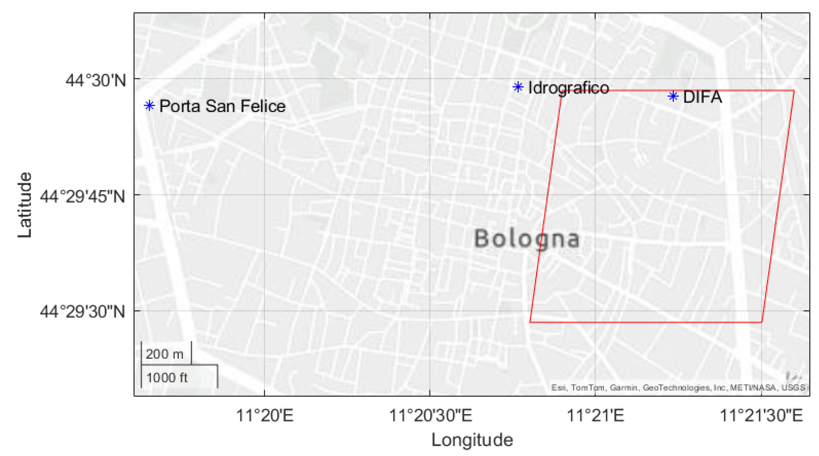
Figure 2.
Daily “wet” PM2.5 from LOAC (blue line) and daily RH from Bologna Idrografico (yellow line). Grey areas refer to days with total precipitation higher than 20 mm.
Figure 2.
Daily “wet” PM2.5 from LOAC (blue line) and daily RH from Bologna Idrografico (yellow line). Grey areas refer to days with total precipitation higher than 20 mm.
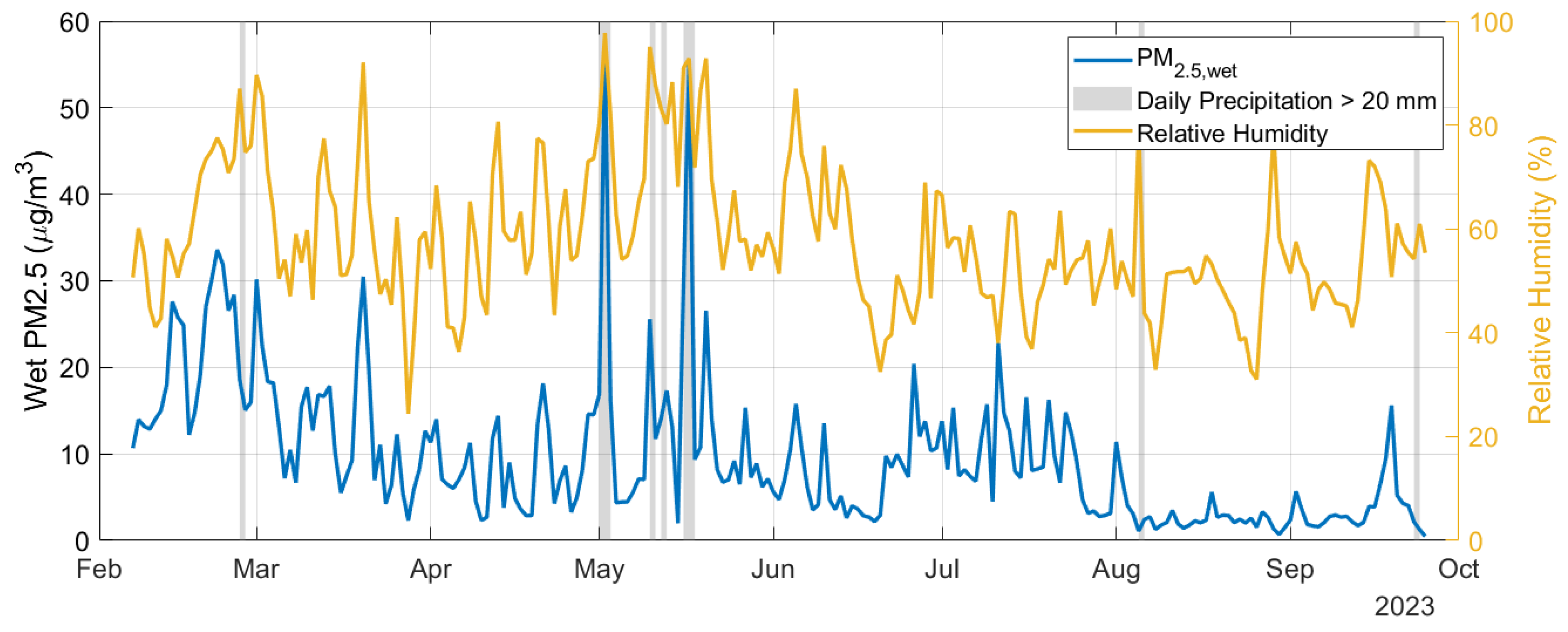
Figure 3.
Monthly PSD averages computed from LOAC PN measurements (logarithmic scales for x and y axis). (a) February to May. (b) June to September.
Figure 3.
Monthly PSD averages computed from LOAC PN measurements (logarithmic scales for x and y axis). (a) February to May. (b) June to September.
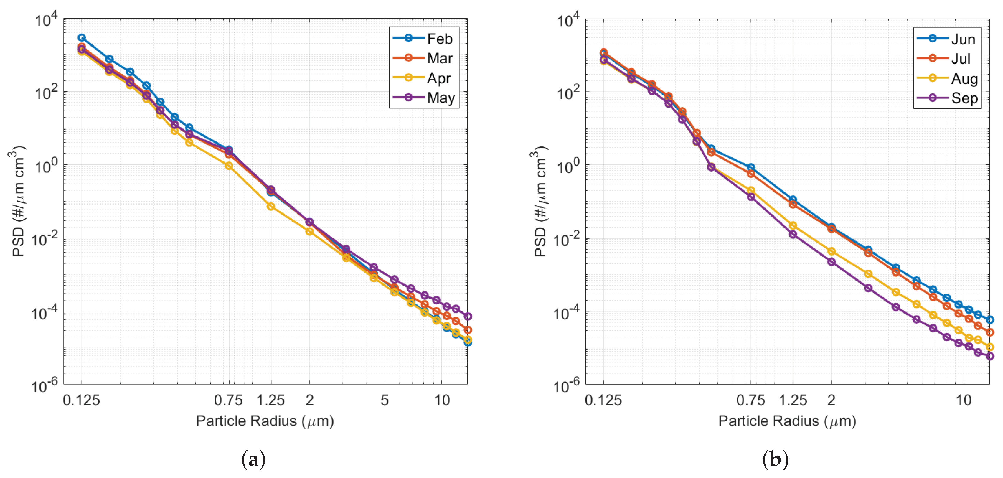
Figure 6.
Results from the linear regressions. (a) Linear regression between and (no auxiliary data). (b) Linear regression between and (daily averages). In the two cases, data points are color-coded with the average hourly and daily RH respectively.
Figure 6.
Results from the linear regressions. (a) Linear regression between and (no auxiliary data). (b) Linear regression between and (daily averages). In the two cases, data points are color-coded with the average hourly and daily RH respectively.
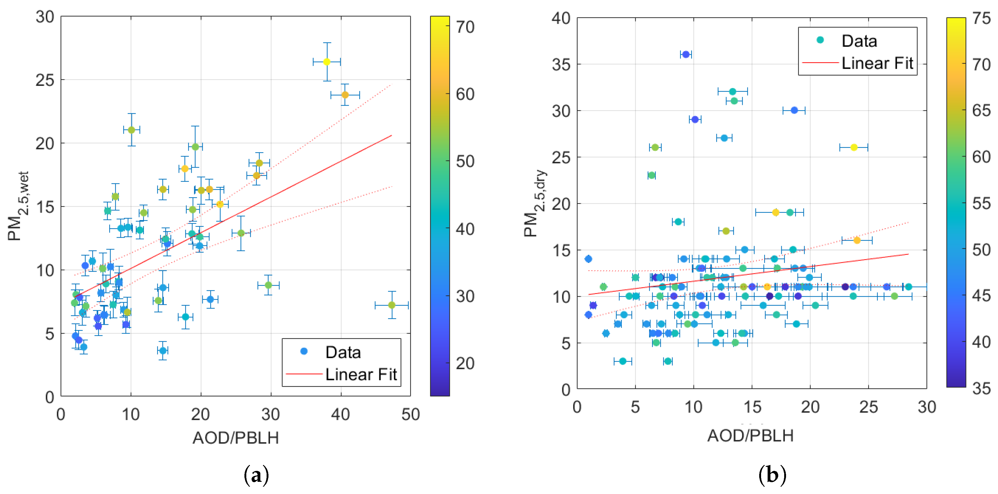
Figure 7.
Results from the linear regressions with auxiliary data. (a) Linear regression between and . (b) Linear regression between and , where is computed with the new values of . In both cases, the data points are color-coded with the respective values of A and .
Figure 7.
Results from the linear regressions with auxiliary data. (a) Linear regression between and . (b) Linear regression between and , where is computed with the new values of . In both cases, the data points are color-coded with the respective values of A and .
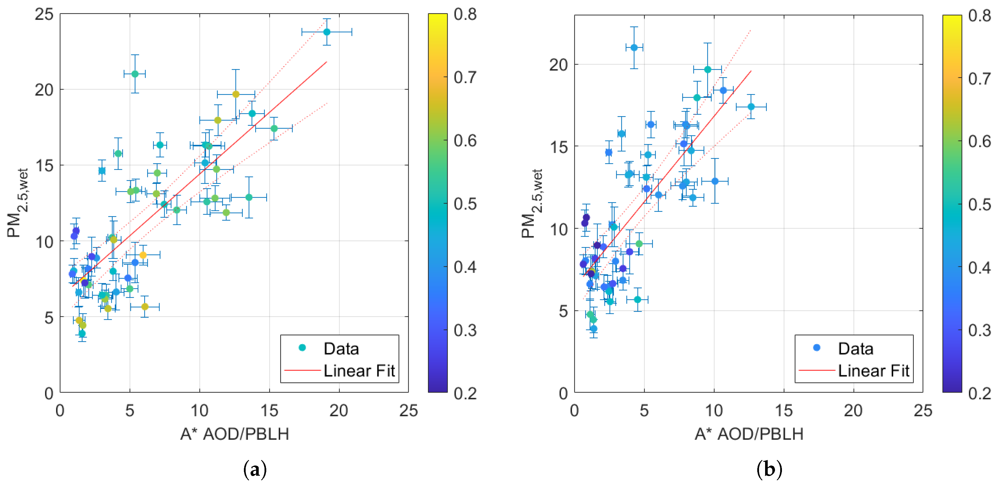

Table 1.
Definition of LOAC size bins, respective bin edges, and average diameters.
| Size bin | Bin Edges () | Bin Diameter () |
|---|---|---|
| 1 | ||
| 2 | ||
| 3 | ||
| 4 | ||
| 5 | ||
| 6 | ||
| 7 | ||
| 8 | ||
| 9 | ||
| 10 | 4 | |
| 11 | ||
| 12 | ||
| 13 | ||
| 14 | ||
| 15 | ||
| 16 | ||
| 17 | ||
| 18 | ||
| 19 |
Table 2.
Size classes of LOAC particle types and respective diameter edges (D).
| Size class | 1 | 2 | 3 | 4 | 5 | 6 |
|---|---|---|---|---|---|---|
| D () |
Table 3.
Results from all the linear regressions with the function , where and . , , and are the parameter A computed respectively with the "new" values of and alone, and with both. The regressions were performed on 49 data points apart from the first, which was performed on 56 data points. The coefficients a and b are listed with relative uncertainty based on 95% confidence bounds.
| X | Definition | R | RMSE () | error | error | |
|---|---|---|---|---|---|---|
| X | 0.5587 | 0.312 | 4.28 | 0.282 + 40% | 7.26 + 26% | |
| 0.7610 | 0.579 | 3.11 | 0.812 ± 24% | 6.27 ± 23% | ||
| 0.7337 | 0.538 | 3.03 | 1.042± 27% | 6.38±23% | ||
| 0.6997 | 0.490 | 3.18 | 0.431 ± 30% | 6.63 ± 24% | ||
| 0.7196 | 0.518 | 3.09 | 0.587 ± 28% | 6.54±23% |
Disclaimer/Publisher’s Note: The statements, opinions and data contained in all publications are solely those of the individual author(s) and contributor(s) and not of MDPI and/or the editor(s). MDPI and/or the editor(s) disclaim responsibility for any injury to people or property resulting from any ideas, methods, instructions or products referred to in the content. |
© 2025 by the authors. Licensee MDPI, Basel, Switzerland. This article is an open access article distributed under the terms and conditions of the Creative Commons Attribution (CC BY) license (http://creativecommons.org/licenses/by/4.0/).
Copyright: This open access article is published under a Creative Commons CC BY 4.0 license, which permit the free download, distribution, and reuse, provided that the author and preprint are cited in any reuse.


