
Submitted:
27 April 2025
Posted:
29 April 2025
You are already at the latest version
Abstract
This study investigates hadronic masses with a focus on scalar/vector mesons and baryons with spins of ℏ2 and 3ℏ2, excluding orbital angular momentum. A novel model based on Kaluza-Klein theory is presented, simulating the Standard Model and expanding it to ten dimensions: one temporal, three spatial, and six compactified. The model proposes that excitations, similar to light-speed ripples in 10D spacetime, generate mass in a 4D universe and exhibit unique spin traits. Parameters are derived from the electron’s g-factor and measured masses of charged leptons, the proton, neutron, and mesons π+,ϕ,ψ,Υ. Crucial parameters include the compactification radius ρ, weak interaction coupling αw, strong interaction coupling αs, and the antineutrino-to-neutrino density ratio δ. Mass calculations for 102 hadrons are performed, with 70 compared to experimental values. A relative error under 0.05 appears in 56% of cases and below 0.1 in 84%, with a correlation coefficient of r=0.997 (p<10−78). Additionally, masses for 32 hadrons are predicted. The model anticipates sterile particles interacting gravitationally, potentially constituting dark matter. The model’s analysis involves the strong, electromagnetic, and weak forces, depicted with equations and figures. Notably, asymmetry in electromagnetic, and to a lesser extent, weak forces might elucidate dark energy.
Keywords:
hadron masses
; Kaluza-Klein theory
; geodesic equation
; Standard Model
; antineu-trino/neutrino density
; fundamental forces (strong
; electromagnetic
; weak)
; neutrino mass
; dark matter
; dark energy
1. Introduction
The Standard Model of particle physics [1,2,3,4,5,6,7] stands as one of the most triumphant theories in the realm of physics. It excels at elucidating the fundamental interactions among particles through bosons [8]: the photon governs electromagnetism, the eight gluons oversee the strong force, and the , and bosons manage the weak force. A significant accomplishment of the Standard Model is its accurate determination of the electron’s anomalous magnetic dipole moment via quantum corrections. Julian Schwinger introduced this as a first-order adjustment to the Dirac equation in 1948 [9]. Subsequently, higher-order corrections achieved an extraordinary concordance between theoretical predictions and experimental data, with accuracy extending to 12 significant figures [10]. Despite its remarkable successes, the Standard Model has important gaps, such as its inability to explain dark matter and dark energy [11], and its exclusion of gravity. Currently, no effective explanation for dark matter and dark energy exists within the Standard Model’s framework. As for gravity, while extensions like quantum gravity theories [12] suggest a spin-2 graviton as a potential mediator, no experimental evidence supports this. Another challenge is its partial success in calculating the masses of mesons and baryons—key components of ordinary matter—and predicting the behavior of unstable particles in high-energy collisions. The Standard Model employs quantum fields in a flat four-dimensional spacetime, whereas general relativity [13] interprets gravity using curved spacetime over cosmic distances, serving as the backbone of contemporary cosmology [14]. However, could a higher-dimensional spacetime offer another way to unify the strong, electromagnetic, and weak interactions without a quantum gravity graviton? The earliest attempt at such a unification was made by Theodor Kaluza in 1921 [15,16], proposing a five-dimensional theory that included electromagnetism. Oskar Klein added the quantum perspective in 1926 [17,18]. A comprehensive summary of these ideas was published in 1987 by Appelquist, Chodos, and Freund in the work *Modern Kaluza-Klein Theories* [19]. Paul Wesson provided an update in 1999 [20], followed by a further update in 2018 [21]. Numerous investigations into Kaluza-Klein theories explore the integration of electromagnetism into a five-dimensional spacetime by frequently developing a corresponding five-dimensional metric and Einstein tensor. Higher-dimensional extensions emerge in string theory [22,23,24], a field rich in mathematical complexity but still lacking testable predictions. Conversely, the Standard Model effectively explains the quantum architecture of elementary particles and predicts their decay probabilities [25], but it does not provide a comprehensive method for calculating hadron masses [26,27]. Consequently, there is a need for an alternative approach that places particle physics within the context of a higher-dimensional spacetime framework. Should one abandon the Standard Model in favor of a theory that adeptly represents gravity yet falters in particle physics? Alternatively, could both the Standard Model and a higher-dimensional relativity coexist as complementary perspectives? Perhaps they are dual facets of a more profound theoretical structure, akin to wave-particle duality. This potential is reminiscent of the renowned double-slit experiment [28], which reveals both wave and particle characteristics. This paper presents a model that reinterprets the Standard Model through a *Kaluza-Klein-like theory*—offering not a contradiction, but a different perspective. The presented framework features ten adaptable dimensions: one temporal, three large-scale spatial, and six compact spatial dimensions. Within this ten-dimensional spacetime, an *excitation*—a transient deformation—consistently travels at the speed of light. In four-dimensional space, such an excitation appears as a gravitational wave, whereas in a compact dimension, a stable excitation has a clearly defined length based on the dimension’s radius. The six compact dimensions’ radii dynamically change according to specific excitations, which relate to particle properties. As the model is developed, the explicit spacetime structure is devised. Further steps involve elucidating the three fundamental interactions and devising formulas for computing particle masses, with particles identified in relation to the six compact dimensions. The model’s essential parameters are determined using empirical data, incorporating the known masses of the charged leptons, the proton, the neutron, and mesons , as well as the electron’s magnetic moment. Key parameters include the compactification radius , the weak coupling constant , the strong coupling constant , the magnetic moment’s constant M, the magnetic field’s constant N, the flavor constants A, and the neutrino-to-antineutrino density ratio . Once established, no further free parameters exist. Subsequently, the model outlines rules for calculating the mass of scalar and vector mesons, along with spin- and spin- baryons without orbital angular momentum. It calculates masses for 102 hadrons, which are then compared to experimental data when available, with the relative error between observed and predicted masses being under 0.05 for most hadrons. The model also accommodates sterile leptons and hadrons, which interact solely through gravitational forces, thus constituting dark matter. Finally, the evaluation of the model includes an analysis of the strong, electric, and weak forces, which are described with equations and illustrations. The electric force, and to a lesser extent the weak force, show asymmetrical behavior, which may offer an explanation for dark energy. Ultimately, to evaluate the model, two experiments conducted in a laboratory setting and one observation from astronomical data are proposed.
2. Methods/Model
2.1. Embedding and Container Space
We begin with a 10-dimensional framework comprising a single time dimension alongside nine spatial dimensions. The familiar concept of spacetime includes the time and three of these spatial dimensions, whereas the six additional dimensions are compactified. To facilitate computation, this 10-dimensional framework is embedded within a 20-dimensional container. The correlation between the 10D spacetime coordinates, , and the coordinates of the container space, , is expressed by:
Here, represents the radius of the compactified dimension. The container space is equipped with a simple flat metric of the form:
where indices range from 0 to 19. The connection between the 10-dimensional physical space and the 20-dimensional container space is expressed as:
This results in a spacetime signature of for the undeformed 10D spacetime. The six compactified dimensions are categorized based on their roles in fundamental interactions: - Strong interaction: dimensions 4 to 6 - Electromagnetic interaction: dimension 7 - Weak interaction: dimensions 8 and 9
2.2. Angular Momentum of a Stable Excitation in a Compactified Dimension
A particle is viewed as an aggregate of associated excitations that move as waves through one or more of the six compactified cylindrical dimensions. The signal speed around any cylinder consistently equals c, the speed of light. Completing one full circuit of a cylinder (encompassing double the typical phase space) is expressed as:
where is an integer and , the wavelength, is linked to the frequency f and the speed of light through the usual formula:
The excitation’s momentum is defined as:
where represents the wave vector. Using these definitions, the spin (angular momentum) of an excitation in a compactified dimension is calculated as:
This outcome does not depend on the cylinder’s radius.
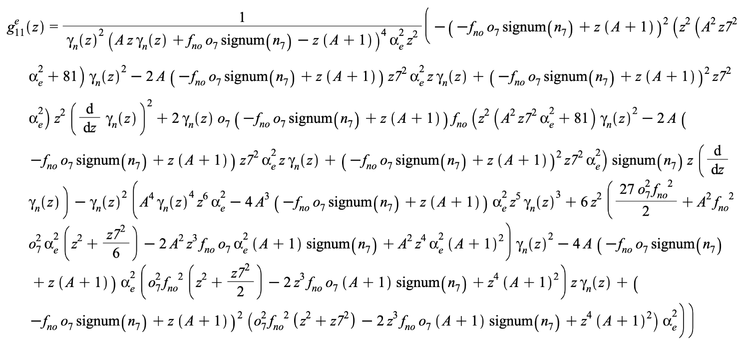
2.3. The Electric Interaction – Dimension 7
The derivation begins with a point-particle current (as observed in four-dimensional spacetime) with four-velocity :
The corresponding covariant Liénard-Wiechert potential [29], generated by a point particle with four-velocity , is given by:
The potential energy between these two particles is:
where is abbreviated as , with being a constant with units of length and z a dimensionless parameter. The invariant form is given by:
where
and
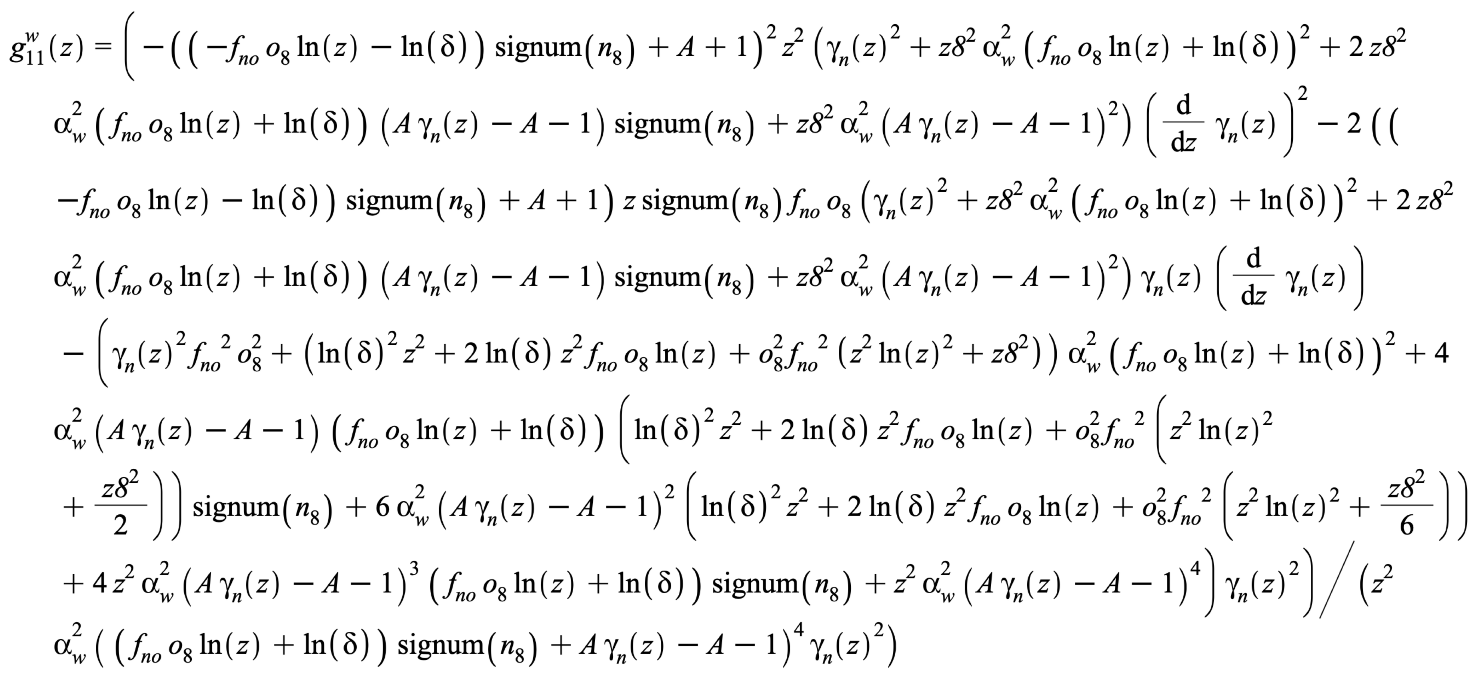
for (see Appendix B.1). The function signum is defined such that . The function encapsulates z-dependent terms, including the metric tensor , the normalized velocity , and the Lorentz factor . The force acting on a particle is given by:
The total electric energy of an excitation consists of rest and kinetic energy:
where the second term represents a constant multiplied by the Lorentz factor . Since total energy is conserved, we obtain:
Solving this differential equation allows us to determine the cylinder radius of dimension 7, where and represent excitation numbers:
In the limit as , the undisturbed radius is given by:
which allows us to fix the constant C as:
where is identified as the compactification radius, which will be determined later. Substituting this into equation (17), we obtain:
Finally, inserting equation (20) into equation (15), the electric energy is given by:
Since mass is obtained by adding potential energy (10) and dividing by , the electric mass is:
which is independent of z. The mass is caused by a excitation with the excitation number , a sinusoidal wave of wavelength . A is interpreted a excitation in form of a standing wave with equal numbered positive and negative excitations. It does not give rise to an additional force or additional spin. Therefore, A is either zero or a positive even number.
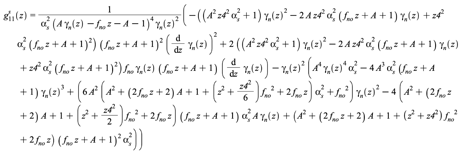
2.4. The Strong Interaction – Dimensions 4, 5, and 6
At this stage, the color representation is introduced as:
For an anti-color, each component is multiplied by . The calculation of the cylinder radii follows the same approach as in the electric case. Again, starting with a point-particle current of four-velocity , the current in each relevant dimension is:
The vector potential, assuming a simplified ansatz [30,31,32,33], depends linearly on the distance between the two color charges:
The potential energy between two particles is then:
The force is given by:
The rest and kinetic color energy of a cylinder excitation follows the same structure as in the electric case:
As before, energy conservation gives:
Solving for the radii of the color cylinders (), we obtain:
The constant is determined by:
which leads to:
Thus, the cylinder radius is:
Without including potential energy, the color energy simplifies to:
Finally, the color mass is:
2.5. The Weak Interaction – Dimensions 8 and 9
The point-particle currents associated with the weak interaction are given by:
In the electric case, the vector potential follows a dependence, while in the strong interaction, it exhibits a linear z dependence. The electric force acts in one dimension, whereas the strong interaction spans three dimensions. The weak interaction, which occupies two dimensions, suggests a logarithmic dependence for the potential as a natural functional form for this number of dimensions:
The associated potential energy, following the same derivation as in previous cases, is given by:
The force acting on a particle is then:
Following the same considerations as in previous cases, the rest and kinetic energy can be expressed as:
As before, total energy conservation requires:
From this, the radius of the compactified weak interaction dimensions () is found to be:
Neutrino Screening Effect
A crucial aspect not previously mentioned is a screening effect due to nearby neutrinos and antineutrinos. Particles interacting via the weak force are influenced by their surrounding neutrino and antineutrino distributions. This means that, in addition to direct interactions with another specific particle, there is an additional contribution from nearby neutrinos and antineutrinos.
Let be the ratio of the average neutrino distance to the average antineutrino distance . This is equivalent to the cubic root of the ratio of antineutrino density to neutrino density . In a homogeneous density, this relationship holds for any given volume V, where:
which gives:
This establishes the neutrino-to-antineutrino distance ratio:
The presence of modifies the undisturbed cylinder radii of the weak interaction. Consequently, fixing the free constant requires:
which leads to the final expression:
The overall neutrino-antineutrino distribution, characterized by , contributes only a small correction to a particle’s energy:
Finally, the weak interaction mass is:
2.6. The Undisturbed Cylinder Radii
The undisturbed radius of a cylinder is its natural radius, unaffected by any potential energy dependent on z. The remaining energy is given by:
which must be nonzero to satisfy energy conservation. Solving for r yields:
The function , which characterizes the interactions, is defined as:
This leads to the following expressions for the undisturbed weak interaction radius:
Role of the Screening Effect
The additional term arises from the weak interaction potential energy (38), where mean distances to neutrinos and antineutrinos play a role:
Since this "potential" is independent of z, it does not contribute to any force.
2.7. The Particle Mass from Strong, Electric, and Weak Interactions
The Lorentz factors for all three interactions at their respective fixed points (see Appendix B.2), where their radii equal the undisturbed radii, are:
For all additional dimensions associated with the strong, electric, and weak interactions, the total particle mass , excluding contributions from "magnetism," is given by:
2.8. Masses Solely Dependent on the Weak Sector
The situation differs for particles affected exclusively by the weak interaction. In this case, only nearby neutrinos and antineutrinos influence the radii of the weak interaction cylinders. As a result, (38) simplifies to:
Consequently, no force acts on the particle:
The excitation energy in the rest frame retains the same structure as in the general weak interaction case (40) but without z dependence:
Since the cylinder radius remains constant, it is given by:
Thus, the excitation energy becomes:
Finally, the corresponding mass for is:
3. Results - Model’s Calculated Values
3.1. Calculation of the Model’s Constants
3.1.1. The Compactification Radius
The time required for an electron excitation (of length and velocity c) to complete one revolution around the cylinder is:
From this, the electric current is calculated as:
The classical magnetic dipole moment, defined with winding number and current loop areaA, is:
For a single electron in the compactified dimension, with , the Bohr magneton, and the z-component of spin (corresponding to the spin of the electric dimension), the magnetic dipole moment is:
By comparing these two expressions and using the measured g-factor of an electron , the compactification radius is determined as:
Having achieved the numerical value of the compactification radius , the g-factor of any Dirac particle can be calculated. With the mass (56) and the generalized particle magneton the g-factor becomes
The g-factor is dependent on the mass of the first generation particles only. In general a particle’s magnetic dipole moment is
3.1.2. The Weak Coupling and the Neutrino Distribution Ratio
The masses of the three charged leptons are calculated using Equation (56) but without an active color charge:
At this stage, the weak coupling and the neutrino distribution ratio are unknown. However, by writing the masses of the electron (71) and the the positron (), assuming
the system allows us to determine and estimate . The experimental upper bound on the positron-electron mass difference,
allows the calculation of an interval with within:
It is known that [36], which agrees well with the result in (74). This supports the assumption that . A second argument supporting this result comes from the higher-dimensional structure of the photon, which will be derived later in this paper. In order for the photon to be massless, the condition must hold.
From this point onward, calculations are performed under the assumption:
To complete the list of lepton constants, the measured masses of the muon and tau, along with Equations (70), are used to determine their values. The results are and . We use , a result that is independently received later (see Table 2). Flavor constants must be zero or even integers. Taking into account the statistical, observational, and numerical errors of the calculation results, the flavor constants are close to integers. However, cannot take a value other than 1. Therefore, the muon is regarded as a superposition of the electron and a respective second-generation lepton, leading to the results, which are used in all further calculations (see Table 1).
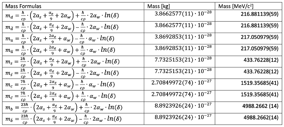
3.1.3. Hadron Mass Formulas
Using Equation (56), the mass contributions from the strong, electric, and weak interactions for quarks can be expressed as:
The differences in quark masses are not solely due to the interaction strengths but are also significantly influenced by the flavor constants . As previously stated, all first-generation constants are set to zero (76). Excluding magnetic field contributions, the first-generation meson masses are given by:
Each quark and antiquark behaves as a dipole and possesses a magnetic field corresponding to each excited compactified dimension but do cancel except for the electric dimension (details see Appendix C). The magnetic field within the compactified dimension is derived from the Biot-Savart law for quarks (A14) and antiquarks (A17) within the compactified electric dimension. The leaking of the magnetic field into 3D space generates mass contributions for mesons
and for baryons
A further mass contribution comes from dipoles within the magnetic fields of the partner quarks/antiquarks with
for mesons, and
for baryons of spin 1/2 and 3/2 (third equation for baryons with identical quark flavors). Mass contributions for mesons and baryons differ due to their internal field interactions.
Meson Mass Formula
Using this framework, the mass formulas for the first-generation mesons are given by:
Baryon Mass Formula
Baryons consist of three quarks and exist, when without orbital rotation, in two spin states: and . For spin , one of the quarks (the p-quark) undergoes a spin flip, breaking the symmetry. As a result, different quark configurations—despite having the same quark content—can lead to different baryon masses. A clear example of this is the mass difference between the (1116 MeV) and the (1193 MeV) baryons, both of which share the quark content . This symmetry breaking, combined with the selection rules given below, alters the calculation of additional mass terms.
Selection Rules for spin -Baryons
- For baryons consisting of a mixture of u-like (u, c, t) and d-like (d, s, b) quarks, the non-flipped quarks always represent a u-d-like combination.
- In case of a baryon consisting of a u-d-mixture built of three different quark species, there always exist two combinations with a different quark flipped. These are baryons with identical excitation numbers but a dissimilar mass.
- For those baryons consisting of purely u- or d-like quarks the non-flipped quark pair consists of different flavors.
For spin baryons, each quark interacts with its two neighboring quarks, making the order of quarks irrelevant. Consequently, each unique quark combination corresponds to a single mass value and all quarks are treated equally. One exception, however, is when 3 identical quarks build one spin -baryon. In this case, an exclusion principle - two identical quarks within one compactified tube only - arranges two quarks within one cylinder and the third quark within a different one.
3.1.4. Mass Formulas for the Proton and Neutron
For a baryon with quark content (proton), where one u-quark is flipped, only one configuration exists. The total mass of the proton is:
Similarly, for the neutron (), where one d-quark is flipped, the mass is given by:
3.1.5. Evaluation of Field Multipliers and Strong Coupling Constant
To determine the field multipliers N and M and the strong coupling constant, which affects the binding energy of hadrons, we utilize the three most accurately measured hadron masses: the charged pion (87), the proton (89), and the neutron (90). Including statistical uncertainties, the values obtained are , , and . These calculations derive solely from the three specified hadrons. The value of N (refer to (82) and (83)) is contingent on an average value of z, whose precise value remains unknown. However, it suffices to understand the relative distance z between baryons and mesons. The calculation of N will thus refine itself. The strong interaction chiefly determines the separation within quarks of baryons and mesons, resulting in in relation to , values utilized for the calculations. Although M is independent of z, it may vary slightly between different particles. Consequently, calculations were performed on all 20 combinations of first-generation particles Proton, Neutron, , , , and , and the standard deviations were computed. These standard deviations are applied in subsequent calculations for N and M. remains unaffected, and the original value is used as shown in Table 2.
3.2. Particle Identification
The identification of fermions is straightforward. Color charge and electric charge are easily assigned:
- A quark carries one of the three colors: red, green, or blue, along with its respective excitation numbers.
-
The electric excitation number is:
- -
- for a down quark
- -
- for an up quark
- -
- for an electron
- Each excitation number contributes a spin of times the excitation number. To ensure an overall spin of , the weak excitations are adjusted accordingly.
- A neutrino consists exclusively of weak excitations and is described as a superposition of weak excitation states. Its excitation number, formally written as , is the same as the weak excitation contribution of a u-quark (see Table 3).
3.2.1. Higher-Generation Particles and Antiparticles
For higher-generation particles, the excitation settings remain identical to those of the first generation. Antiparticles are obtained by multiplying all excitation numbers by .
3.2.2. Excitation Numbers of Photons and Gluons
The excitation numbers of the Standard Model gauge bosons can be inferred from known decay processes. For example, in electron-positron annihilation [37], two photons are produced:
This corresponds to the following excitation number transformation:
Two real, measurable photons are created. As follows using Equation (62), photons are massless. A related example is the meson, which has a decay mode producing three gluons [38]:
highlights the structure of a gluon and shows the correspondence with the excitation numbers transformation:
The Standard Model of Particle Physics explains that the main interaction among quarks within hadrons results from gluon exchange. According to this Kaluza-Klein perspective, the strong force emerges due to the curvature of spacetime. Taking into account both the Standard Model and the Kaluza-Klein model as complementary frameworks, the gluon mass within hadrons can be interpreted as:
Using the evolution equation [3] to scale up to -boson energy, we obtain:
for three colors () and five flavors (). The Particle Data Group (PDG) reports the strong coupling at the energy scale as , demonstrating excellent agreement with the model’s prediction.
3.2.3. Summary of Gauge Bosons
In Table 4, the photon and the color-altering gluons (distinct from the eight gluons in the Standard Model) are delineated. The , , and bosons are not highlighted, as they seem to exert minimal influence on the calculation of the hadron masses.
3.2.4. Mass Generation via Compactified Dimensions
In this model, mass arises from excitations of the compactified dimensions. - Excitations always travel at the speed of light in higher dimensions. - When an excitation is projected into 4D spacetime, it manifests as mass. Thus, particles gain their mass due to their interaction within higher dimensions.
3.3. Hadron Masses
The field multipliers and coupling constants are assumed to be independent of particle generation. The quark flavor constants are determined using the known formulas and the measured masses of the , and mesons.
The flavor constants are calculated solving the system of three equations (95) with the results: , , and . It is assumed that flavor constants are the result of standing waves within the compactified cylinders, meaning equal numbers of positive and negative excitation numbers. Therefore, those numbers must be even. However, the s-quark is regarded as a superposition of the d and the respective quark of the second generation with . Taking statistical, observational, and numerical errors of the calculation results into account, the flavor constants are
These values then allow for the calculation of hadron masses. First, the masses of scalar and vector mesons are computed, followed by the masses of baryons with spin and . The reference list of particles was primarily obtained from Wikipedia [39,40], where the lowest mass states for each quark combination are listed. However, it is not entirely clear whether these values, particularly for baryons, are the most suitable for comparison. Nevertheless, the measured particle masses listed in these sources are used for comparison against the calculated values, and to estimate the relative error caused by uncertainties in determined masses. All other calculations are based on the latest data from the Particle Data Group (PDG) [34]. The tables presented in this section include:
- Particle name and symbol
- Quark content
- Measured and calculated masses (in and )
- Standard deviations
- Relative error
- Mass formula used for the calculation
The measured masses in kilograms are provided without standard deviations, as these values are not used in subsequent calculations.
3.3.1. Meson Masses
For scalar mesons, the quark and antiquark spins are aligned antiparallel, resulting in a net spin of . The corresponding masses are listed in Table 6.
For vector mesons, the quark and antiquark spins are aligned parallel, leading to a net spin of . The corresponding masses are presented in Table 7.
3.3.2. Baryon Masses
A baryon consists of three quarks, each with spin . If one quark undergoes a spin flip, the resulting baryon has a total spin of (Table 8). The masses are calculated using equation (88).
If all three quarks, each with spin , align in the same direction, the baryon has a total spin of (Table 9).
3.4. Correlation Between Measured and Calculated Hadron Masses
3.5. Sterile Dirac Particles
Equation (56) indicates the plausible existence of Sterile Leptons and Sterile Quarks, characterized by engaging in direct interaction with the couplings, bypassing a possible dependence on charges. With appropriate conditions, a Sterile Dirac Particle might be formed via a collision, possibly resulting in a mass given by
, where is zero or a positive even integer, the sum of the positive and negative excitation numbers with and . Sterile particles interact solely through gravity.
3.6. Calculation of Particle Acceleration and Force
In a coordinate system with the two interacting particles aligned along the -axis with , the velocity is expressed as a function depending on the separation between the particles. Employing the metric tensor from Equation (3), the Christoffel symbols are calculated in the standard manner by summing over repeated indices from 0 to 9:
The acceleration is then determined using the geodesic equation:
The forces exerted on the particle can be described by:
The energies involved are of equations (21), (34), and (48).
3.7. The Constant Scalar
In conventional four-dimensional spacetime, the velocity four-vector is defined as:
where it adheres to the conservation relation:
Within a 10-dimensional spacetime, the conservation principle extends based on the quantity of compact active dimensions :
The additional dimensions are indexed as .
The computation of force is feasible solely when the function is available. Thankfully, it stays the same since its derivative is zero, indicating that it is constant.
This result aligns with Newton’s third law, , and is evidently zero since the derivative of equation (102) is zero. The value of is determined when both particles are stationary, ensuring its validity at any speed. Specifically, for charged leptons, we find:
, where denotes contributions from the two weak dimensions in superposition. For quarks located within a baryon relative to one of the other two accompanying quarks, we find:
, and in the context of quarks inside a meson:
, where (with ) pertain to active color contributions, and reflects the effect of weak interactions. The invariant’s result remains constant but varies for distinct particle types:
3.8. Coulomb Force Between Two Slowly Moving Charges
The calculation of the electric force between two charges, and is performed for slowly movement, where , and is used. The radius expression from Equation (20) simplifies to:
is the energy of Equation (21), and it interacts with the Christoffel symbols. Although solving Equation (99) completely is intricate, the initial terms of the series expansion in are still tractable:
where is the physical distance in meters. Since is on the order of a femtometer, for distances above , the first term in Equation (109) dominates. This term is equivalent to the well-known Coulomb force formula from classical electrostatics:
where and represent the two charges, and is the vacuum permittivity.
3.9. Force Calculations and Asymptotic Behavior
By establishing the invariant expression (refer to Equations (11) and (103)) and acknowledging its uniformity across particle types, the model provides for the direct computation of the strong, electric, and weak forces. These forces are influenced by the particle’s velocity, which can be approximated using the Uncertainty Principle. Quarks are localized to an area around with , leading to
The estimated velocity of the quark, based on the masses provided in Appendix Table A2, is detailed in Table 11.
The equations are expressed as functions involving z, which represents the normalized distance separating the particles. The Figure 2, Figure 3, and Figure 4 illustrate the forces, with , and the normalized particle velocity.
Strong Force
Electric Force
Weak Force
An unforeseen result is the asymmetric influence of the electric and weak forces on d- and u-quarks within nucleons (see Figure 5). The electric force disparity amounts to at , whereas the weak force difference at the same point amounts to just .
An intriguing outcome is the repulsion observed between particles with differing electric charges when they are in close proximity and moving at velocity, as illustrated in Figure 6. Consider an example of an electron-positron collision occurring at a velocity , corresponding to an invariant mass of .
This electric repulsion remains consistent whether dealing with electron-positron pairs or electron-electron/positron-positron combinations, up to a distance of roughly (Figure 7):
The scenario was computed assuming a constant velocity. However, due to the repulsion, the velocity decreases, which leads to the attraction between the electron and positron taking effect at a greater distance than depicted in the example.
3.9.1. Key Results on Force Strengths
-
Strong Force:
- -
- Predominant within hadrons.
- -
-
Attractive Forces:
- *
- Baryons: Exerts at for d- and u-quarks, much lower for other quarks.
- *
- Mesons: Displays at per compactified dimension for d- and u-quarks, considerably weaker for other quarks.
- -
-
Repulsive Force characteristics occur for:
- *
- (baryons).
- *
- (mesons).
-
Electric force:
- -
- Inside hadrons: when .
- -
- At the value , the force surpasses .
- -
- No matter the charge configuration, the force is consistently repulsive over the range , which significantly relies on the particles’ speed. For instance, in the case illustrated by Figure 6 and Figure 7, involving a collision with an invariant mass of leading to a velocity of , the range is . However, deceleration was not taken into account, hence, attraction will commence sooner.
-
Weak force:
- -
- when .
- -
- when .
- -
- The force is repulsive if the charge signs differ, and otherwise attractive.
3.9.2. Asymmetric Forces in Electric and Weak Interactions of -Hadrons
In quark combinations, the electric force and, to a lesser extent, the weak force manifest asymmetrically. This results in a disparity where the force exerted on a d-quark differs from that on a u-quark (refer to Figure 5). Without rotational motion, these quarks exhibit a type of Zitterbewegung, distinct from the electron’s Zitterbewegung [41]. Conversely, if rotational motion occurs, the hadron engages in a sort of random walk [38].
3.9.3. Particle Transformation in Collision Processes
Up to this point, the discussion of collision processes has been omitted in this article. In the Standard Model of Particle Physics, particle formation is explained via boson exchange mechanisms (involving photons, Z, W, and Higgs bosons) or through vector meson exchange. Within this Kaluza-Klein Model, transformation of particles occurs when the colliding particles come to rest and merge. A commonly recognized process is the conversion of a - pair into a - pair, described by:
accompanied by the excitation table:
The dynamics of this process are exclusively governed by electromagnetic forces. As demonstrated in Figure 6 and Figure 7, collisions between electrons and positrons exhibit a repulsive interaction, resulting in deceleration and eventual merging. The complexity of equation (113) has hindered detailed computation of the process, wherein the deceleration affects the velocities of the leptons, modifying the force as function of z and . Implementing a numerical iterative method could potentially provide insights into the detailed transmutation.
4. Discussion
The described Kaluza-Klein analogue employs the fundamental version of a Calabi-Yau manifold [42], characterized in this context by a 10-dimensional spacetime organized in the following manner:
- One dimension for time
- Three standard spatial dimensions
- Six compactified dimensions, each shaped like perpendicular cylinders.
In this 10D spacetime, there are no strings or additional elements; instead, it acts as a structural framework where disturbances propagate at light speed, altering the topology and breaching Ricci flatness [43]. Most disturbances are transient ripples within the 10D spacetime; however, some become stable excitations within the compactified dimensions, manifesting as particles in 4D spacetime yet still traveling at light speed in 10D. A stable excitation within a compactified dimension of radius r can be viewed as a sinusoidal wave with a wavelength , which adheres to condition (4). By employing de Broglie’s formula [44], one can describe the energy of a stable excitation, which enables summarization of the total energy of a hadron as comprising:
- Excitation energies
- Potential energies
- Contributions from magnetic fields and dipoles
4.1. Hadron Masses
Using Einstein’s energy-mass equivalence, one can compute meson and baryon masses. In 56% of the comparisons, the relative error between observed and predicted masses is below 0.05, while 84% show errors under 0.1. The model is grounded in the framework of the Standard Model of particle physics, encompassing the three foundational interactions—strong, electromagnetic, and weak—while extending the mathematical principles of general relativity to 10 dimensions. Thus, gravity plays an integral role within this framework. The model stipulates that the six compactified dimensions account for the strong (dimensions 4–6), electromagnetic (dimension 7), and weak (dimensions 8 & 9) interactions. Within this framework, stable waves around compactified cylinders emerge naturally and constitute the primary source of mass. A significant portion of a particle’s mass, particularly for the light quarks, originates from the magnetic field of the compactified dimension 7. For example, the mass contributions from magnetic fields and dipole interactions are:
- Proton (): 31%
- Neutron (): 31%
- Lambda (): 18%
- Bottom Xi (): 2%
- Charged rho (): 40%
- Upsilon (): 0.06%
The field constants N, M, and the strong coupling constant were determined using the most precisely measured hadron masses, namely those of the pion plus, proton, and neutron. However, certain first-generation meson masses still show minor discrepancies between measured and calculated values.
Additionally, spin- baryons consisting of three different quark flavors can exist with two slightly different masses. This model successfully accounts for these differences. For example, the and baryons share the same quark content () but exhibit different masses—a difference the model is able to calculate. Within this model, the potential to generate sterile hadrons and leptons (96), which could be a candidate for dark matter, emerges.
4.2. Summarizing the Fundamental Constants
During the development of this model, it was both possible and necessary to determine several important physical constants (Table A1):
- The compactification radius:
- The weak coupling constant:
- The strong coupling constant:
- The neutrino distribution ratio:
- The constant scalar:
- The flavor constants:
The parameter arises from the two compactified weak-interaction dimensions and exhibits a logarithmic dependence on the particle’s mean distance towards neutrinos and antineutrinos. Consequently, is responsible for the extremely low neutrino mass.
From the maximum possible mass difference between the positron and electron, an upper limit on the lightest neutrino mass is derived:
It remains uncertain what the masses of the second- and third-generation neutrinos might be. However, the upper bound aligns with previous estimates:
Further theoretical and experimental work is required to explore potential spatial variations in neutrino-to-antineutrino ratios. If such differences exist, they might be measurable through extremely small variations in fundamental particle properties, such as:
- Electron mass
- Magnetic moment
4.3. Force Calculations and Metric Tensors
In general relativity, the tensor formalism is applied individually to each type of interaction. This distinction is vital as the masses influenced by strong, electric, or weak forces are dictated solely by the corresponding metric tensors. However, quarks experience all three interactions concurrently. Rather than a unified calculation, Equation (99) is used to perform three distinct force calculations, each tailored to one interaction. The outputs offer the specific force equations and graphical depictions found in Section 3.9. Aggregating these forces determines the net force on a particle. Furthermore, the invariant function (Section 3.7) is found to be constant but varies among different particle types. Thus, in this model, all interactions emerge purely from the curvature of a 10-dimensional spacetime. The asymmetric nature of the electric force results in continuous movement resembling a random walk. However, matter bonds through multiple forces, particularly the strong force, overall electric force, and gravitational force. Consequently, the random walk of hadrons does not lead to disintegration. Yet, a significant cumulative force might cause matter clusters to dislodge from one another, potentially explaining the phenomenon referred to as dark energy.
4.4. Two Possible Laboratory Experiments and One Astronomical Measurement to Assess the Model
The Kaluza-Klein model offers insights regarding sterile particles and force interactions. To evaluate the model’s validity, two laboratory experiments and a cosmological observation are proposed:
4.4.1. Creation of Dark Matter
Dynamic interactions among particles are expected to generate sterile particles (96). In this framework, rapid incoming particles need to decelerate to unite and form sterile particles. A process with a comparably low invariant mass that could yield sterile particles is as follows:
with the excitation table:
The mass of the sterile particle S is expected to be
To ensure the stability of a sterile particle, the invariant mass of the initial electron-positron pair must match the mass permissible for a sterile particle; otherwise, it would decay into particles that interact through strong, and/or electromagnetic and weak forces. Table 12 lists the invariant masses associated with sterile particles generated in experiments where the initial mass is under .
An experiment conducted to scan the energy range from to is expected to detect an increased missing mass near the resonances at those specific mass values.
4.4.2. Nucleon’s Random Walk
Inside nucleons, we observe quark compositions made of one u-quark and one d-quark, primarily bound by the strong force but also subject to electric and weak forces. The strong interaction exerts an equal influence on both quarks, whereas the electric and weak forces exert differing degrees of force. Consequently, nucleons may undergo a sort of erratic motion [47]. This dynamic differs from Brownian motion [48], which describes how a fluid exerts thermodynamic effects on a suspended small object. The movement of nucleons occurs on a much smaller scale , with their frequency given by . This renders directly measuring an individual nucleon improbable. Nevertheless, a group of ultra-cold polarized neutrons could exhibit some secondary random walk behavior.
4.4.3. Decreasing Strength of Dark Energy
The process of hadronization, which involves the formation of protons and neutrons, began approximately seconds following the Big Bang [49,50,51]. If protons and neutrons, as hypothesized, engage in a random walk (Section 3.9.2), this behavior might contribute to galaxies drifting apart. Although the exact timeline and specifics are not covered in this discussion, if the random walk is essentially synonymous with what is termed as dark energy, then it must diminish as matter transitions into sterile particles (Section 3.5), essentially becoming dark matter. Consequently, the proportion of matter to dark matter would shift in favor of dark matter. This would lead to a reduction in the rate of galactic acceleration. The initial indication of a deceleration is offered by the Euclid space telescope [52]. Additional information is expected to be obtained when the Vera C. Rubin Observatory and Nancy Grace Roman Space Telescope become operational.
4.5. Open Questions
Mass Formula
The mass of a hadron is expressed as the sum of its excitation energy, potential energy, and the energies arising from the magnetic field and magnetic moments in the electric dimension. The influences from both significant (strong dimensions) and minor (weak dimensions) magnetic sources are disregarded, based on the assumption that the contributions from two dominant dimensions negate each other, just as the effects from weak dimensions do. This is inferred because including contributions from the strong or weak dimensions would lead to mass values significantly diverging from observed measurements. Nonetheless, there are still observed differences between the calculated and experimental masses that remain unexplained.
Sterile Masses
The standard expression for sterile particles is presented in equation (96). The premise underlying the computation leading to the data in Table 12 is that surplus energy is confined within two out of the three dimensions of strong interaction. Nonetheless, alternative configurations for energy storage are feasible. Should missing mass resonances manifest in other energy sectors, the approach to energy storage must be adjusted while adhering to (96).
Deceleration in Particle Collisions
When electrons and positrons collide, they exhibit deceleration, though the specifics of this mechanism remain unclear. The complexity of Equation (113), due to its reliance on variables z and , obstructs straightforward calculations. Nonetheless, employing a numerical iterative approach may elucidate the exact mechanisms underlying the collision. Notably, investigating the emergence of the weak interaction at elevated beam energies could provide significant insights.
Computation of Flavor Constants
The derivation of flavor constants begins with the equations for the rest and kinetic energies of the compactified cylinder, given by (15), (28), and (40), expressed as
An alternative formulation
can be considered. This approach modifies the mass of a particle without magnetic effects from
While this modification does not affect first-generation particles, it causes a slight mass shift for second and third-generation particles, with this shift being smaller than the predicted uncertainties.
4.6. Future Applications
Until now, this model has primarily focused on calculating hadron mass and forces, with less attention to particle collisions or creation processes and no consideration of decay processes. Nevertheless, this model might also effectively detail particle creation and decay dynamics — possibly without the need to use Feynman diagrams [53]. Undoubtedly, additional theoretical and experimental studies are needed to thoroughly examine the potential and constraints of this method.
5. Conclusion
The objective of this project began as the calculation of hadron masses. It soon became apparent that certain missing constants needed determination. The values for , the compactification radius; , the weak coupling constant; , the strong coupling constant; , the neutrino distribution ratio, enabling mass calculation. The model additionally provided a way to derive formulas for sterile particles, which interact gravitationally alone—specifically, dark matter. An experiment was proposed to assess the concept (Section 4.4.1). Moreover, once the invariant function was derived, this method facilitated the calculation of the strong, electromagnetic, and weak forces. An unexpected observation was the asymmetrical behavior of the electric force, and to a lesser extent, the weak force, possibly causing a random walk movement in particles with -quark combinations. An experiment is proposed (Section 4.4.2). This phenomenon might contribute to the accelerated separation of galaxies, a phenomenon attributed to dark energy. Here a astronomical measurement is proposed (Section 4.4.3). If the predictions of the model prove to be accurate, the implications are vast. It suggests that an expanding force, resulting from the random walk of nucleons, existed abundantly after the big bang. This likely generated an immense force that separated masses. Simultaneously, collision processes were frequent, leading, as the model suggests, to the widespread creation of dark matter, which reduced ordinary matter in favor of dark matter. Therefore, for this model to hold, a decrease in the cosmological parameter is necessary. Moreover, the future of the universe is also noteworthy because as the proportion of normal matter to dark matter shifts in favor of dark matter, gravity may eventually dominate, leading to a potential final rebound. This could result in a cyclic universe.
Funding
This research received no external funding
Acknowledgments
The successful completion of this study was greatly supported by the use of sophisticated computational tools, essential for handling the complex and voluminous equations encountered. The software tools Maple and StatFree played crucial roles in this process.
Conflicts of Interest
The author declares no conflicts of interest.
Appendix A
Appendix A.1. Statistical Error Analysis
The statistical deviations of the calculated constants, as well as quark and hadron masses, are derived using Gaussian error propagation (A1):
Equation (A1) computes the standard deviation of a quantity Z, which is calculated from parameters given as mean values and their corresponding standard deviations. This method is applied to the numerical results of Equations (67), (74), () and the data presented in Table 2, Table 6, Table 7, Table 8, Table 9, Table A1, and Table A2.
Appendix A.2. Parameters Calculated Within the Model

Table A1.
List of Model’s Derived Constants
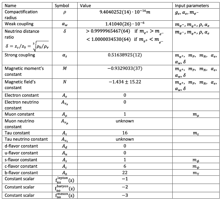
Table A2.
Quark Masses (Excluding Magnetic Contributions). While quarks and antiquarks have distinct masses, this variance is less than the error margin arising from parameter imprecision of the input measurements.
Table A2.
Quark Masses (Excluding Magnetic Contributions). While quarks and antiquarks have distinct masses, this variance is less than the error margin arising from parameter imprecision of the input measurements.
Appendix A.3. Parameters from Literature Used in the Calculations
Table A3.
Measured Particle Masses Used in the Calculations [34]
Table A3.
Measured Particle Masses Used in the Calculations [34]
| Particle | Symbol | Mass (kg) | Mass (MeV/) |
|---|---|---|---|
| Electron/Positron | e | ||
| Muon | |||
| Tau | |||
| Pion+ | |||
| Proton | P | ||
| Neutron | N | ||
| Phi Meson | |||
| J/Psi Meson | |||
| Upsilon Meson |
Table A4.
Constants from Literature Used in the Calculations [34]
Table A4.
Constants from Literature Used in the Calculations [34]
| Constant | Symbol | Value |
|---|---|---|
| Speed of light | c | 299792458 m/s |
| Reduced Planck constant | Js | |
| Electron’s spin g-factor | ||
| Electric coupling constant |
Appendix B
Appendix B.1. Coordinates and Velocities Within the Ten Dimensions
The coordinate origin is chosen to be at the location of the entangled partner particle. Thus, represents the normalized distance between two entangled particles. Only the relative distance between the two particles is of interest; therefore, the coordinate system’s -axis is aligned along the direction of the particle, while the other two spatial coordinates are set to zero.
Within the compact dimensions, a stable excitation is distributed over the entire cycle . A particular location along a compactified coordinate is defined as follows, where and with representing the intersection of the higher-dimensional space with the 4D-spacetime:
The velocity in three-dimensional space is less than c for massive particles (as induced by higher dimensions) but equals the speed of light for photons and excitations of 4D spacetime, gravitational waves. In the compactified dimensions, the velocity is always equal to the speed of light.
Appendix B.2. Lorentz Factors of Strong, Electric, and Weak Interactions at Their Fixed Points
The velocities corresponding to the fixed points for each of the three interactions are considered individually. These fixed points represent the initial conditions where a particle begins to be affected by the respective forces when its velocity is zero, thus:
Appendix B.3. The Metric Tensor
The components of the metric tensor are influenced by the distance to the nearest particle and, to a lesser extent, by the average distances to the nearest neutrino and anti-neutrino. However, the latter effect is negligible and therefore omitted in the following equations. There exist three metric tensors, one for each interaction, with the general form:
For , all off-diagonal elements approach zero, and the diagonal component satisfies . The metric components can be calculated directly using equation (3). Each interaction-specific mass couples only to its respective Christoffel symbol. For instance, in the case of the electric interaction, the only nonzero off-diagonal elements are . Additionally, the diagonal elements differ for each interaction, as indicated in equation (A5):
 The off-diagonal elements take the following forms:
Here, the indices 4, 7, and 8 on z correspond to the compactified dimensions’ contravariant coordinate indices.
The off-diagonal elements take the following forms:
Here, the indices 4, 7, and 8 on z correspond to the compactified dimensions’ contravariant coordinate indices.
Appendix C. Magnetism
The Biot-Savart law in three-dimensional space is given by:
Here, the denominator accounts for the weakening of the magnetic field as a function of distance R from the dipole. However, in a compactified dimension, the magnetic field remains confined within the curled-up dimension, where no such weakening occurs. As a result, the equation modifies to:
which simplifies to:
where:
and denotes the angle on the compactified dimension.
A similar equation holds for the antiquark, with the substitution . Since quarks and antiquarks share a common compactified dimension but with a phase shift of , the corresponding magnetic field is:
Thus, when a quark’s magnetic field is multiplied with the magnetic field of an antiquark a normalizing factor is necessary:
Magnetic Effects on the Masses of Leptons, Mesons, and Baryons
The additional mass contribution due to the magnetic field leaking into three-dimensional spacetime for lepton pairs and mesons is given by:
Evaluating the integral, we obtain:
For baryons, the additional mass due to the magnetic fields is:
Evaluating this integral:
In both expressions (A19) and (A21), the parameter N represents the magnetic field constant, which absorbed the term . This constant is determined by solving the system of equations (87) (charged pion), (89) (proton), and (90) (neutron), which at the same time provides the numerical values of the constants M and .
Another contribution to the hadron mass arises from the dipole moment (69) of a quark within the magnetic field of its partner quark:
Magnetic Dipole Contribution to Mesons and Lepton Pairs
The additional mass due to the dipole moment is given by:
Here, M is the magnetic moment constant. The term in the denominator ensures dimensional consistency, while making M dimensionless and is the normalizing factor.
Magnetic Dipole Contribution to Baryon Mass
For baryons, the additional mass contribution due to dipole interactions is:
Here, the first equation is valid for spin-1/2 baryons, the second for spin-3/2 baryons with at least two different quark flavors, and the third for spin-3/2 baryons with quarks of the same flavor.
Weak and Strong Magnetism
Given that all compactified dimensions exhibit comparable structures, it stands to reason to anticipate that magnetism could arise from the weak and strong dimensions. However, the effective range of these forces is exceedingly limited, suggesting the absence of magnetic fields originating from the strong and weak dimensions. Calculations of these magnetic fields, based on analogies with the magnetism linked to the electric force, produce values significantly higher than those inferred from empirical data. In both the strong and weak forces, there are two identical contributions, which appear to neutralize one another.
References
- Goldberg, D. The standard model in a nutshell; Princeton University Press, 2017.
- Langacker, P. The standard model and beyond; Taylor & Francis, 2017.
- Thomson, M. Modern particle physics; Cambridge University Press, 2013.
- Vergados, J.D. The standard model and beyond; World Scientific, 2017.
- Bettini, A. Introduction to elementary particle physics; Cambridge University Press, 2024.
- Griffiths, D.J. Introduction to elementary particles. Physics textbook, 2010.
- Cottingham, W.N.; Greenwood, D.A. An introduction to the standard model of particle physics; Cambridge university press, 2007.
- Jaeger, G. Exchange forces in particle physics. Foundations of Physics 2021, 51, 13. [CrossRef]
- Schwinger, J. On quantum-electrodynamics and the magnetic moment of the electron. Physical Review 1948, 73, 416. [CrossRef]
- Aoyama, T.; Hayakawa, M.; Kinoshita, T.; Nio, M. Tenth-order electron anomalous magnetic moment: Contribution of diagrams without closed lepton loops. Physical Review D 2015, 91, 033006. [CrossRef]
- Wang, B.; Abdalla, E.; Atrio-Barandela, F.; Pavon, D. Dark matter and dark energy interactions: theoretical challenges, cosmological implications and observational signatures. Reports on Progress in Physics 2016, 79, 096901. [CrossRef]
- Rovelli, C. Quantum gravity; Cambridge university press, 2004.
- Einstein, A. Die Grundlagen der allgemeinen Relativitatstheorie. Annalen der Physik 1916, 49, 769.
- Weinberg, S. Cosmology; OUP Oxford, 2008.
- Kaluza, T. Zum unitätsproblem der physik. Sitzungsber. Preuss. Akad. Wiss. Berlin (Math. Phys.) 1921, 1921, 966–972.
- Kaluza, T. On the problem of unity in physics. Unified Field Theories of> 4 Dimensions 1983, p. 427.
- Klein, O. Quantentheorie und fünfdimensionale Relativitätstheorie. Zeitschrift für Physik 1926, 37, 895–906.
- Klein, O. The atomicity of electricity as a quantum theory law. Nature 1926, 118, 516–516. [CrossRef]
- Appelquist, T.; Chodos, A.; Freund, P.G.O. Modern Kaluza-Klein Theories; Addison-Wesley Publishing Company, Inc., 1987.
- Wesson, P. Space-time-matter: modern Kaluza-Klein theory 1999.
- Wesson, P.S.; Overduin, J.M. Principles of Space-Time-Matter: Cosmology, Particles and Waves in Five Dimensions; World Scientific, 2018.
- Witten, E. String theory dynamics in various dimensions. Nuclear Physics B 1995, 443, 85–126. [CrossRef]
- Zwiebach, B. A first course in string theory; Cambridge university press, 2004.
- Polchinski, J. String Theory: Volume 1: An Introduction to the Bosonic String; Vol. 1, Cambridge Monographs on Mathematical Physics, Cambridge University Press: Cambridge, 1998. [CrossRef]
- Urbanowski, K. Decay law of relativistic particles: quantum theory meets special relativity. Physics Letters B 2014, 737, 346–351. [CrossRef]
- DeGrand, T.; Jaffe, R.; Johnson, K.; Kiskis, J. Masses and other parameters of the light hadrons. Physical Review D 1975, 12, 2060. [CrossRef]
- Palazzi, P. Particles and shells. arXiv preprint physics/0301074 2003.
- Carnal, O.; Mlynek, J. Young’s double-slit experiment with atoms: A simple atom interferometer. Physical review letters 1991, 66, 2689. [CrossRef]
- Wiechert, E. Elektrodynamische elementargesetze. Annalen der Physik 1901, 309, 667–689. [CrossRef]
- Ishii, N.; Aoki, S.; Hatsuda, T. Nuclear force from lattice QCD. Physical review letters 2007, 99, 022001. [CrossRef]
- Aoki, S.; Hatsuda, T.; Ishii, N. Theoretical foundation of the nuclear force in QCD and its applications to central and tensor forces in quenched lattice QCD simulations. Progress of theoretical physics 2010, 123, 89–128. [CrossRef]
- Schröder, Y. The static potential in QCD to two loops. Physics Letters B 1999, 447, 321–326. [CrossRef]
- Anzai, C.; Kiyo, Y.; Sumino, Y. Static QCD potential at three-loop order. Physical review letters 2010, 104, 112003. [CrossRef]
- A Zyla, P.; M Barnett, R.; Beringer, J.; Dahl, O.; D Dwyer, A.; D Groom, E.; Lin, C.J.; S Lugovsky, K.; Pianori, E.; D Robinson, J. Review of particle physics (RPP 2020). PROGRESS OF THEORETICAL AND EXPERIMENTAL PHYSICS 2020, 2020, 1–2093.
- Tiesinga, E.; Mohr, P.J.; Newell, D.B.; Taylor, B.N. CODATA recommended values of the fundamental physical constants: 2018. Journal of physical and chemical reference data 2021, 50. [CrossRef]
- R., N. Coupling Constants for the Fundamental Forces, 2025.
- Berends, F.A.; Kleiss, R. Distributions for electron-positron annihilation into two and three photons. Nuclear Physics B 1981, 186, 22–34. [CrossRef]
- Besson, D.; Henderson, S.; Pedlar, T.; Cronin-Hennessy, D.; Gao, K.; Gong, D.; Hietala, J.; Kubota, Y.; Klein, T.; Lang, B. Measurement of the direct photon momentum spectrum in Υ (1 S), Υ (2 S), and Υ (3 S) decays. Physical Review D—Particles, Fields, Gravitation, and Cosmology 2006, 74, 012003.
- Wikipedia, t.f.e. List of mesons. Wikipedia 2025.
- Wikipedia, t.f.e. List of baryons. Wikipedia 2025.
- Hestenes, D. The zitterbewegung interpretation of quantum mechanics. Foundations of Physics 1990, 20, 1213–1232. [CrossRef]
- Yau, S.T.; Nadis, S.J. The shape of inner space: String theory and the geometry of the universe’s hidden dimensions; Il Saggiatore, 2010.
- Misner, C.W.; Thorne, K.S.; Wheeler, J.A. Gravitation; W. H. Freeman and company: San Francisco, 1973; p. 1088.
- De Broglie, L. The reinterpretation of wave mechanics. Foundations of physics 1970, 1, 5–15.
- Aker, M.; Altenmüller, K.; Arenz, M.; Babutzka, M.; Barrett, J.; Bauer, S.; Beck, M.; Beglarian, A.; Behrens, J.; Bergmann, T. Improved upper limit on the neutrino mass from a direct kinematic method by KATRIN. Physical review letters 2019, 123, 221802. [CrossRef]
- Vikhlinin, A.; Kravtsov, A.; Burenin, R.; Ebeling, H.; Forman, W.; Hornstrup, A.; Jones, C.; Murray, S.; Nagai, D.; Quintana, H. Chandra cluster cosmology project III: cosmological parameter constraints. The Astrophysical Journal 2009, 692, 1060.
- Xia, F.; Liu, J.; Nie, H.; Fu, Y.; Wan, L.; Kong, X. Random Walks: A Review of Algorithms and Applications. IEEE Transactions on Emerging Topics in Computational Intelligence 2020, 4, 95–107. [CrossRef]
- Einstein, A. Über die von der molekularkinetischen Theorie der Wärme geforderte Bewegung von in ruhenden Flüssigkeiten suspendierten Teilchen. Annalen der physik 1905, 4. [CrossRef]
- Alpher, R.A.; Bethe, H.; Gamow, G. The origin of chemical elements. Physical Review 1948, 73, 803.
- Fields, B.D., Big Bang Nucleosynthesis: Nuclear Physics in the Early Universe. In Handbook of Nuclear Physics; Springer, 2023; pp. 3379–3405.
- Planck, P.C. results. VI. Cosmological parameters. arXiv preprint arXiv:1807.06209 2018, 34.
- Collaboration, D.; Adame, A.G.; Aguilar, J.; Ahlen, S.; Alam, S.; Alexander, D.M.; Alvarez, M.; Alves, O.; Anand, A.; Andrade, U.; et al. DESI 2024 VI: Cosmological Constraints from the Measurements of Baryon Acoustic Oscillations, 2024, [arXiv:astro-ph.CO/2404.03002]. [CrossRef]
- Gamow, G. Physics and Feynman’s Diagrams. Scientific American 1956.
Figure 1.
Correlation Between Measured and Calculated Masses. The diagonal line represents the ideal case where measured and calculated masses are identical.
Figure 1.
Correlation Between Measured and Calculated Masses. The diagonal line represents the ideal case where measured and calculated masses are identical.
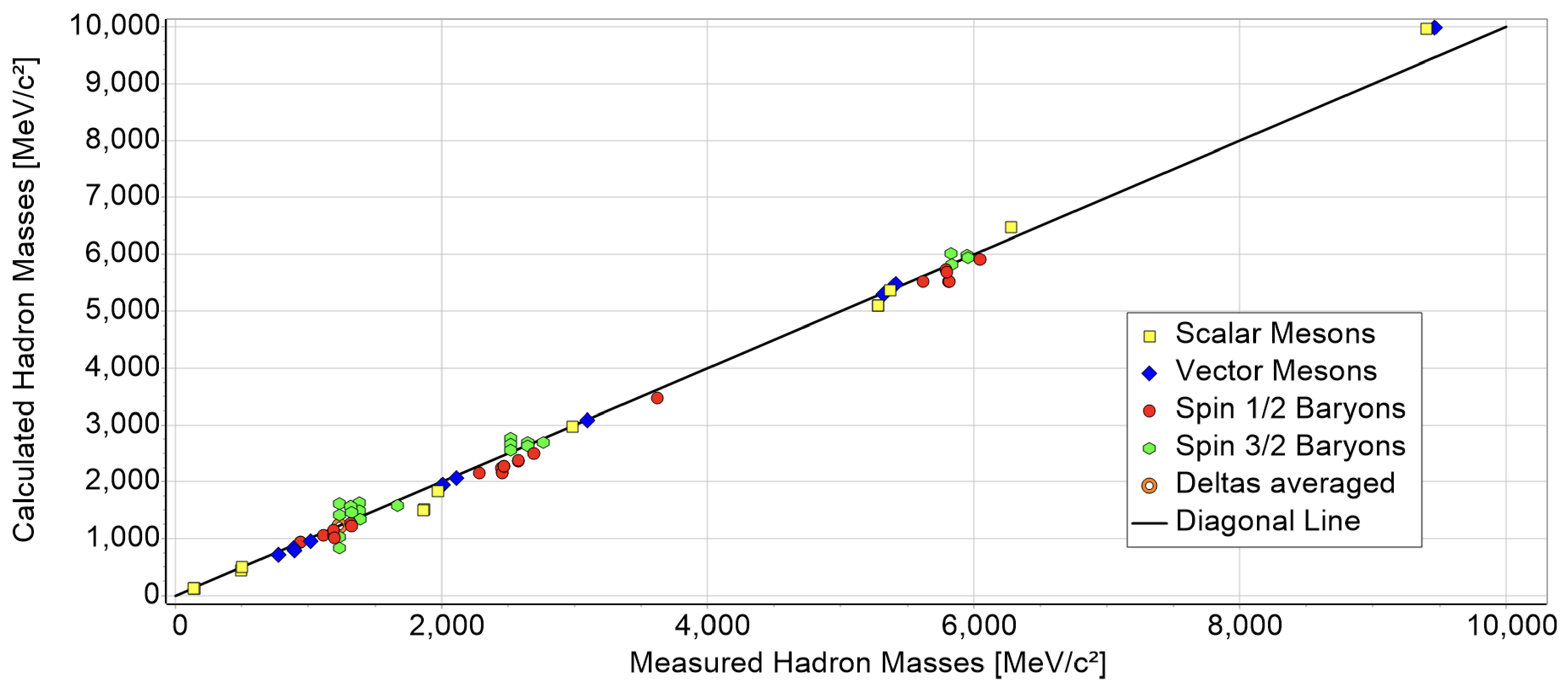
Figure 2.
Strong Force between two Quarks within Baryons.
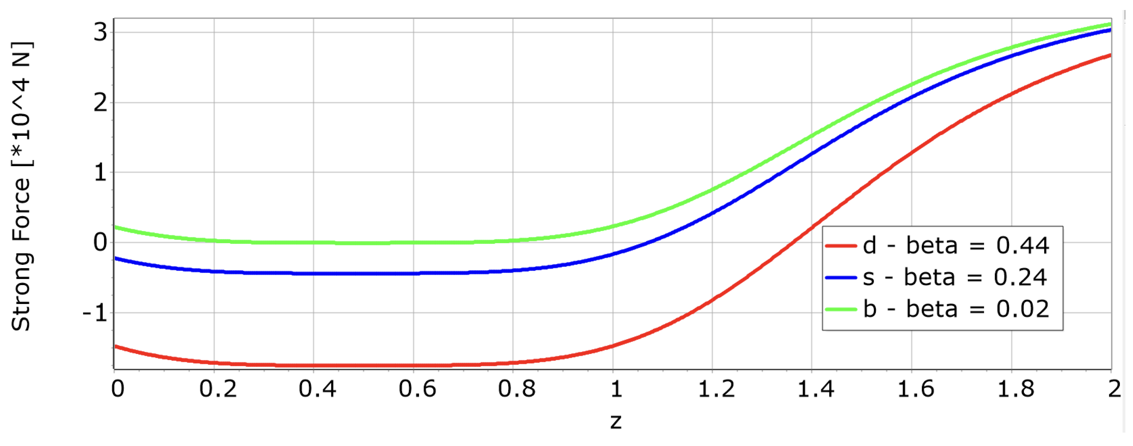
Figure 3.
Electric Force acting on a d/s/b-Quark interacting with a u/c/t-Quark inside a Baryon.
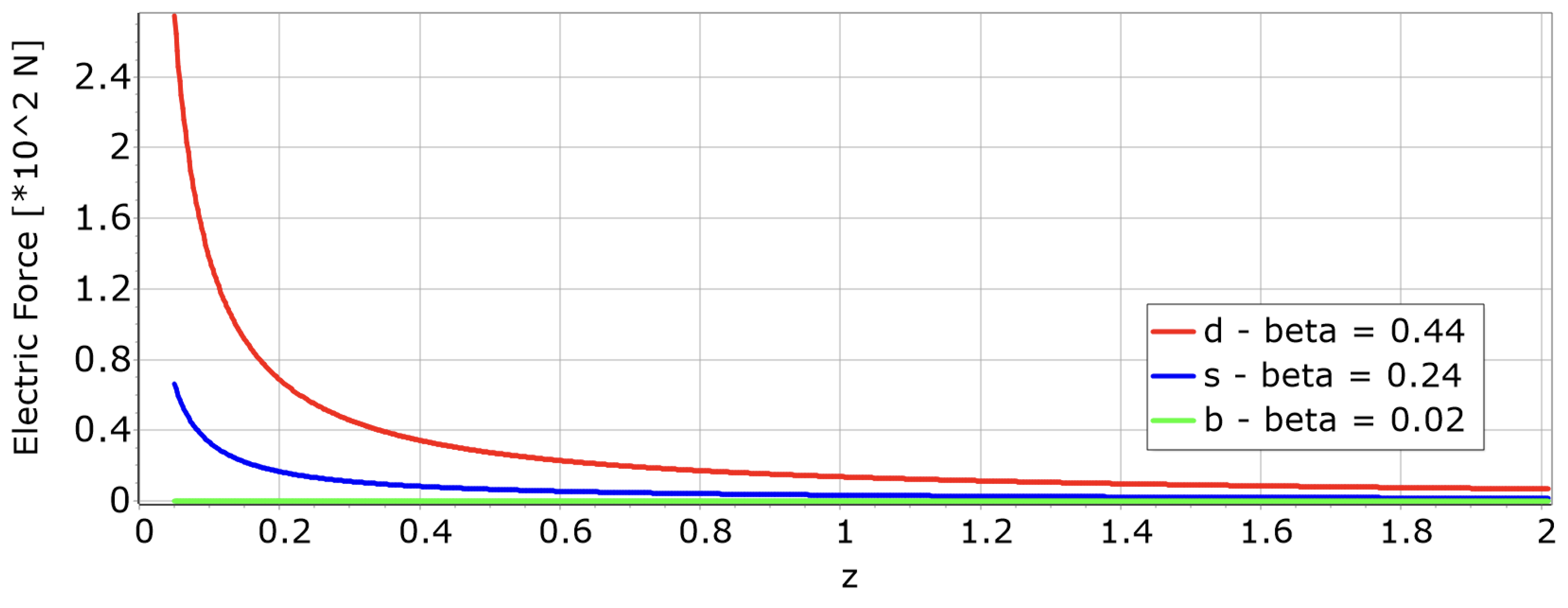
Figure 4.
Weak Force acting on a d/s/b-Quark interacting with a u/c/t-Quark inside a Baryon.
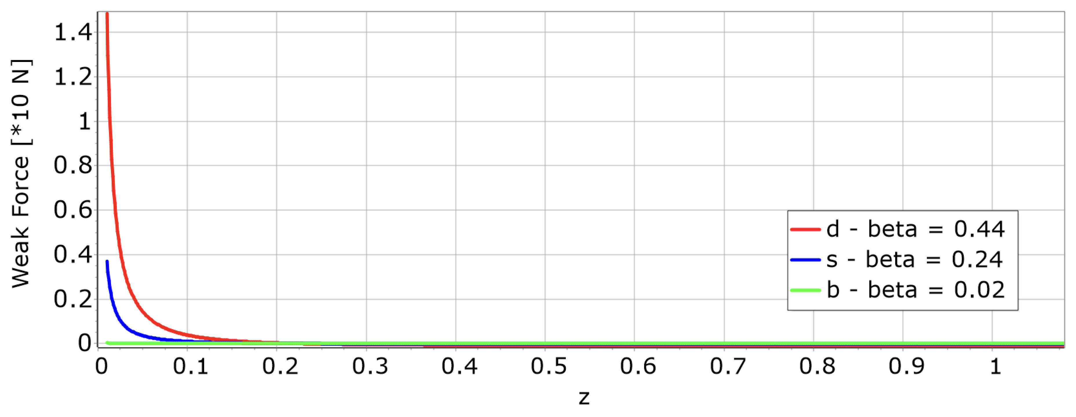
Figure 5.
Electric force exerted on a u-quark when it interacts with a d-quark, and vice versa, within a baryon.
Figure 5.
Electric force exerted on a u-quark when it interacts with a d-quark, and vice versa, within a baryon.
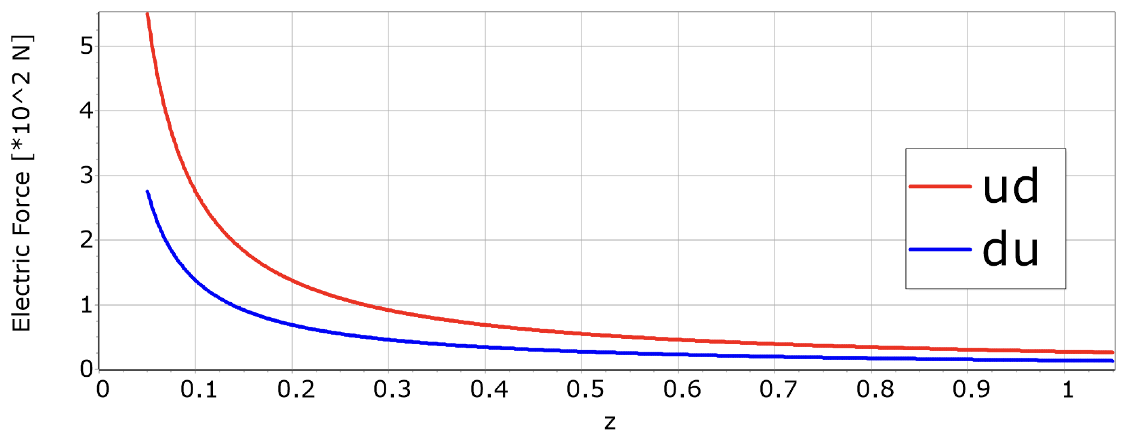
Figure 6.
Electromagnetic interactions involving pairs and pairs at an invariant mass of are depicted for the range .
Figure 6.
Electromagnetic interactions involving pairs and pairs at an invariant mass of are depicted for the range .
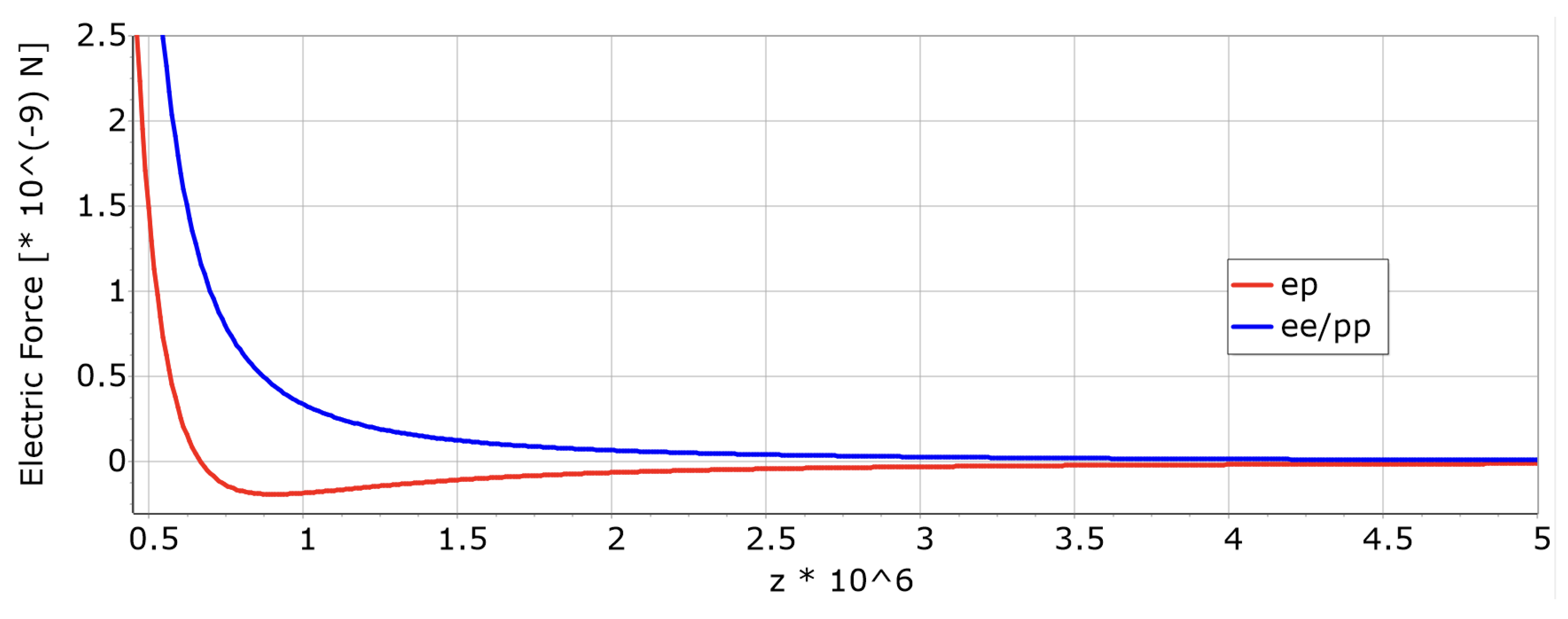
Figure 7.
Electromagnetic interactions among and are analyzed at an invariant mass of , within the range .
Figure 7.
Electromagnetic interactions among and are analyzed at an invariant mass of , within the range .
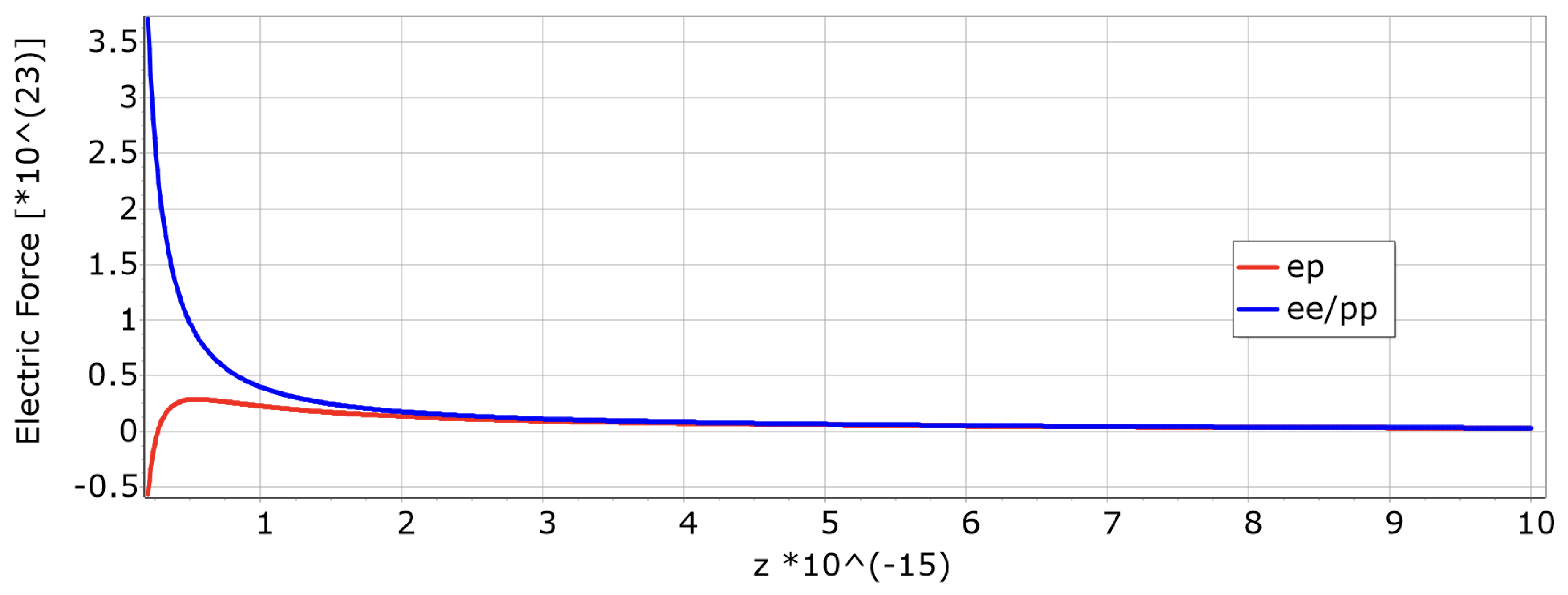
Table 1.
Lepton Constants
| unknown | unknown |
Table 2.
Field Multiplier Values and Strong Coupling Constant
Table 3.
Fermions of the First Generation
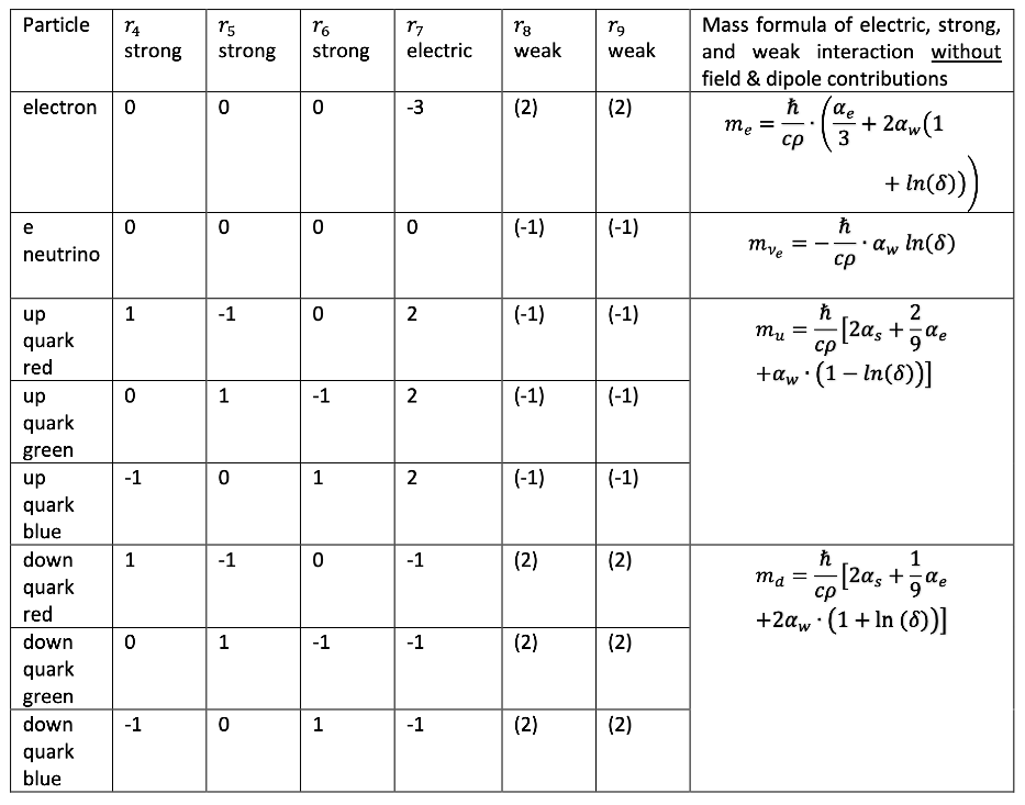
Table 4.
Intermediate Bosons
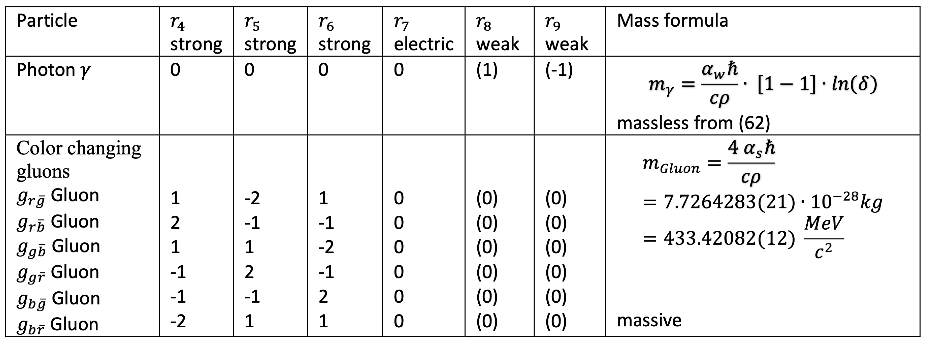
Table 5.
Flavor Constants
Table 6.
Masses of Scalar Mesons
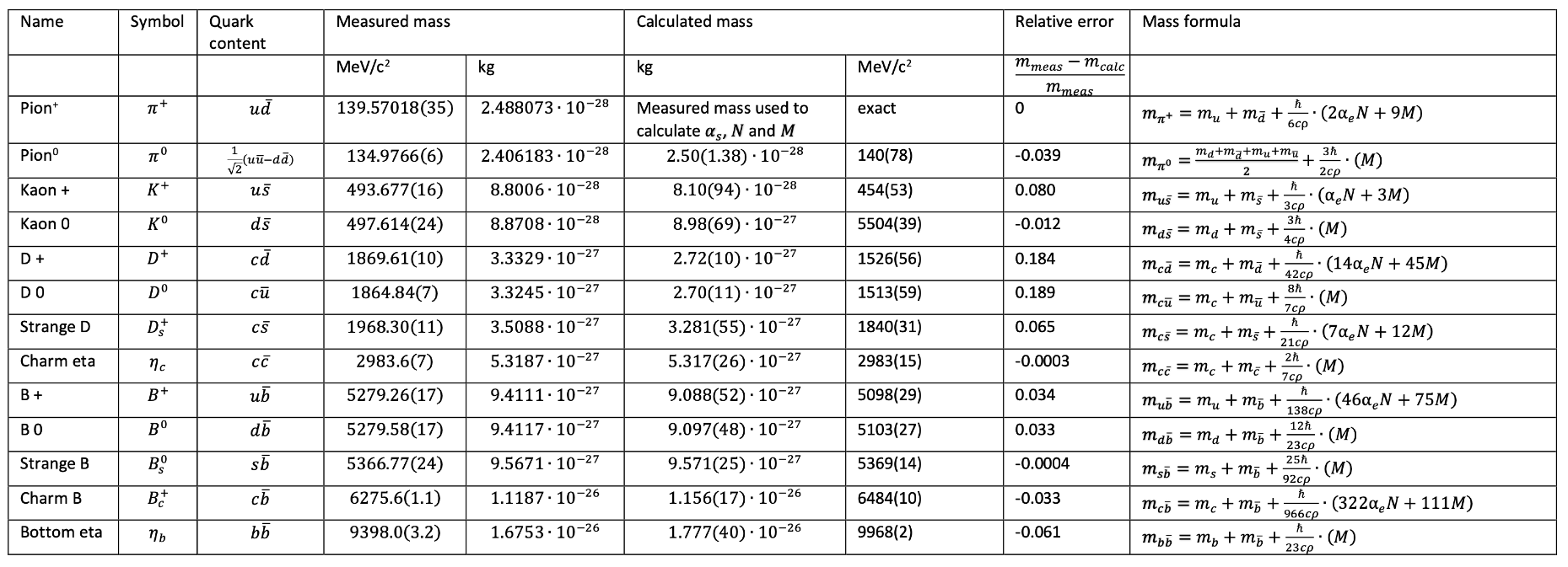
Table 7.
Masses of Vector Mesons
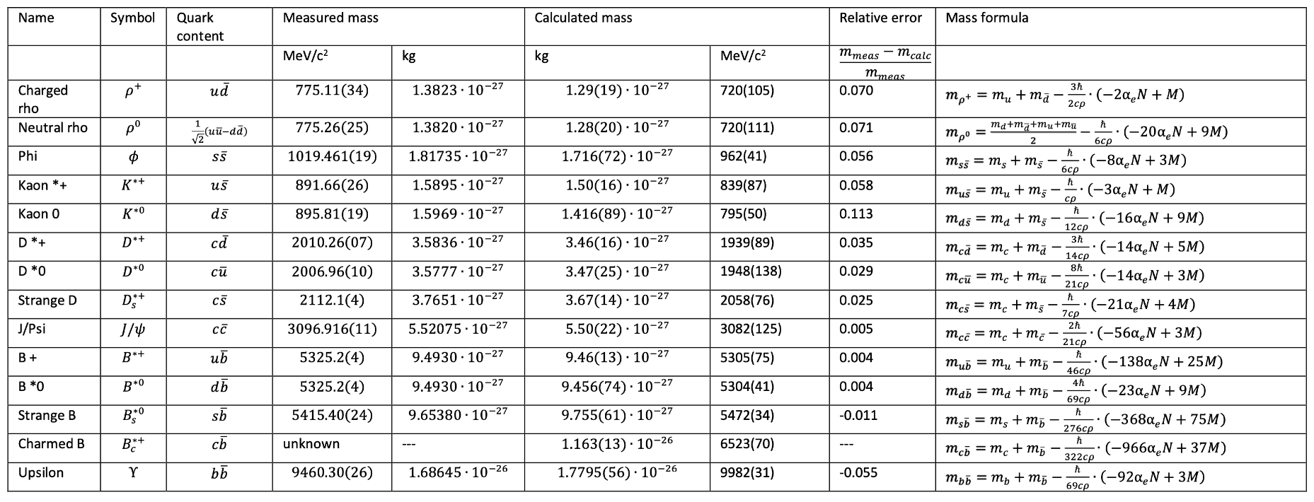
Table 8.
Masses of Baryons with Spin
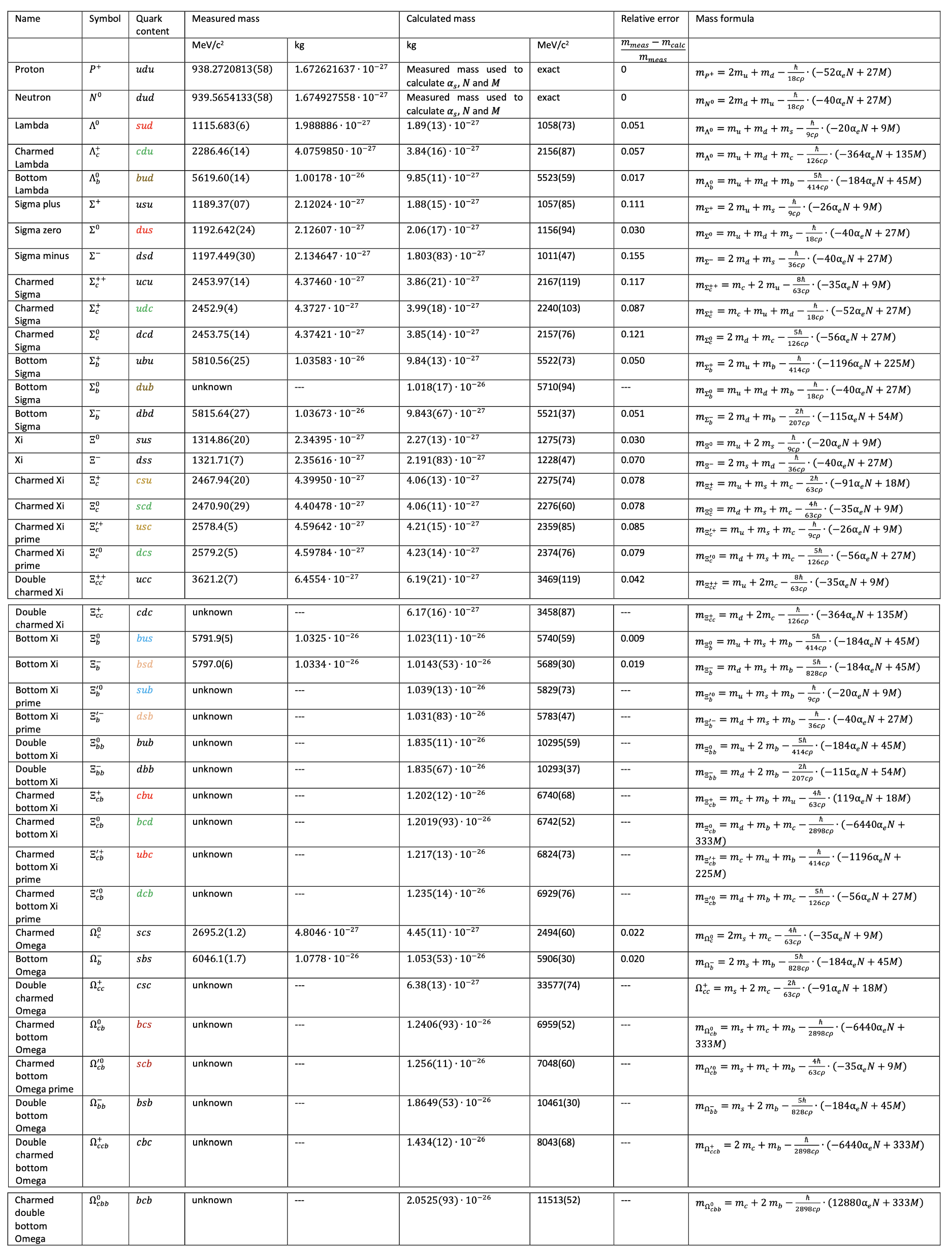
Table 9.
Masses of Baryons with Spin
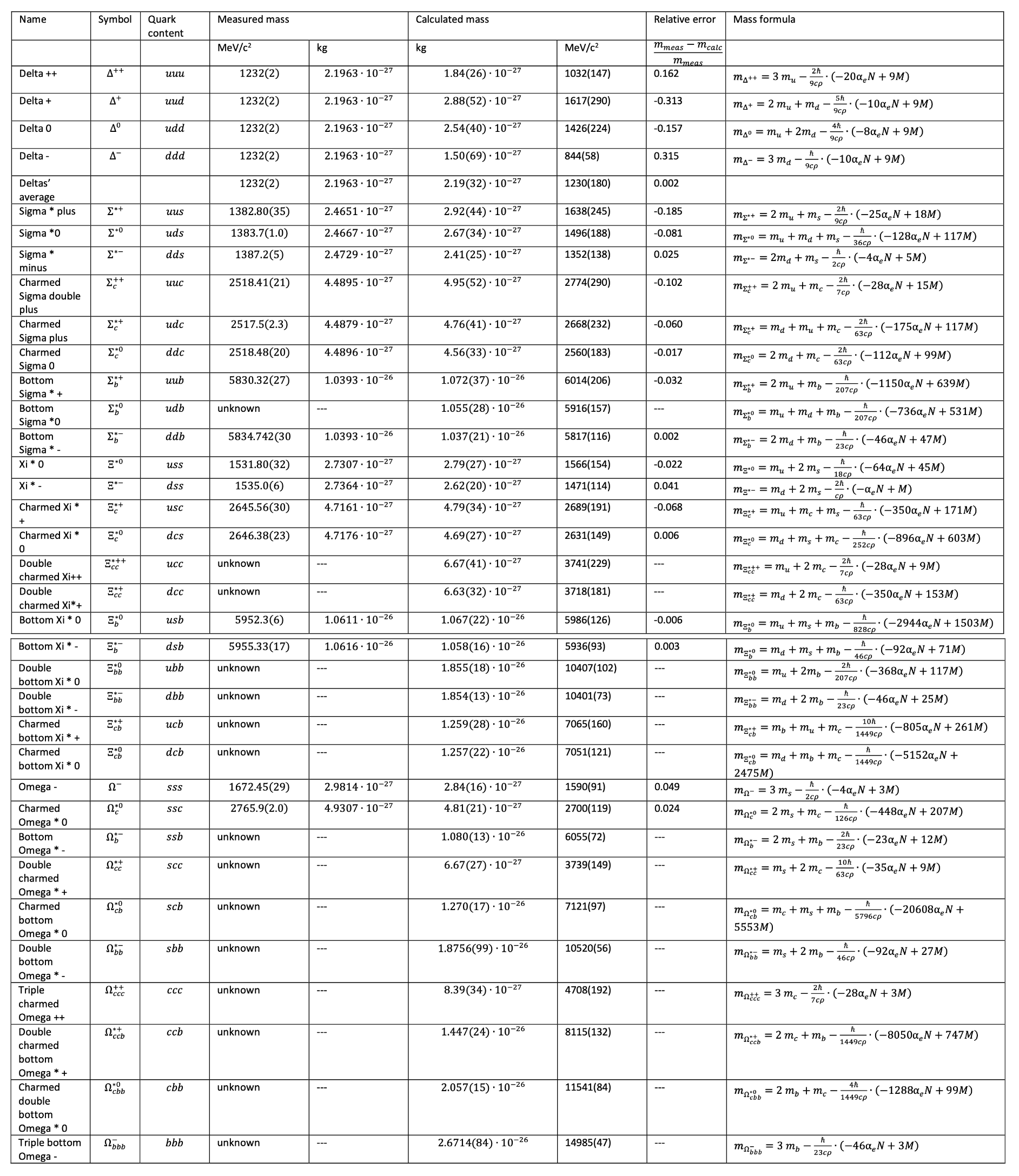
Table 10.
Pearson’s Correlation Between Measured and Calculated Hadron Masses. The table presents Pearson’s correlation coefficient r and the associated significance p.
Table 10.
Pearson’s Correlation Between Measured and Calculated Hadron Masses. The table presents Pearson’s correlation coefficient r and the associated significance p.
| Number of Hadrons | Particle Group | Pearson’s r | p |
|---|---|---|---|
| 13 | Scalar Mesons | 0.998 | |
| 13 | Vector Mesons | 0.999 | |
| 24 | Spin- Baryons | 0.999 | |
| 20 | Spin- Baryons | 0.998 |
Table 11.
Approximated Velocity of Quarks within Baryons
| Quark | Mass | Flavor Constant A | ||
|---|---|---|---|---|
| d | 216.9 | 0.44 | 1.112 | 0 |
| u | 217.1 | 0.44 | 1.112 | 0 |
| s | 433.8 | 0.24 | 1.029 | 1 |
| c | 1519.4 | 0.07 | 1.002 | 6 |
| b | 4988.3 | 0.02 | 1.000 | 22 |
Table 12.
Invariant Masses of light Sterile Particles
| n | ||
|---|---|---|
| 1 | ||
| 2 | ||
| 3 | ||
| 4 | ||
| 5 |
Disclaimer/Publisher’s Note: The statements, opinions and data contained in all publications are solely those of the individual author(s) and contributor(s) and not of MDPI and/or the editor(s). MDPI and/or the editor(s) disclaim responsibility for any injury to people or property resulting from any ideas, methods, instructions or products referred to in the content. |
© 2025 by the authors. Licensee MDPI, Basel, Switzerland. This article is an open access article distributed under the terms and conditions of the Creative Commons Attribution (CC BY) license (http://creativecommons.org/licenses/by/4.0/).
Copyright: This open access article is published under a Creative Commons CC BY 4.0 license, which permit the free download, distribution, and reuse, provided that the author and preprint are cited in any reuse.


