
Submitted:
28 April 2025
Posted:
28 April 2025
You are already at the latest version
Abstract
Articles have recently been circulating in the media around the world, claiming that natural CO2 sinks have “suddenly and unexpectedly” ceased to function. It turned out that these articles were based on a single preprint of a meanwhile published article. Its reasoning is essentially based on the large spike of CO2 concentration growth in 2023 despite constant anthropogenic emissions. However, there are no obvious indications that photosynthesis or oceanic sinks have decreased. In this paper, it is shown that besides the natural sink systems of the land plants and oceans, also the variability of natural emissions has to be considered. Based on a previous publication, it is made evident that natural emissions are temperature-dependent. Therefore, the careful analysis of monthly sea surface temperature and CO2-concentration data 2023 and 2024 gives a consistent explanation for the rise of atmospheric carbon concentration growth without referring to the implausible hypothesis of failing carbon sinks.
Keywords:
Natural CO2 sinks
; Climate change
; Natural emissions
; Temperature dependence
1. Introduction
Articles are currently being circulated in the media claiming that natural CO sinks have “suddenly and unexpectedly” ceased to function, such as the article in the British magazine Guardian: “Trees and land absorbed almost no CO last year. Is nature’s carbon sink failing?“[1]. The natural CO reservoirs are the biological world, consisting of all living organisms, plants, animals and humans. In addition, the oceans, which store around 50 times the amount of atmospherical CO. It is known and has been proven for many decades that both the biological world and the oceans are strong CO sinks. Currently, more than half of all anthropogenic emissions are absorbed by the two major sink systems, ocean and land plants, as reported in [2].
What has happened that suddenly the sink effect is supposedly diminishing? Even at first glance, the diagram (Figure 3) in [2] reveals that the sink effect, which is attributed to land plants, is subject to extraordinarily strong fluctuations, much more so than in the case of the oceans, for example. This should immediately make us suspicious when we talk about a “one-off” event within the past year.
A closer look at all the articles published on this topic quickly reveals that they all refer to a single publication. The scientific basis and trigger for the current discussion is the recent article: “Low latency carbon budget analysis reveals a large decline of the land carbon sink in 2023“ ([3]). The publication essentially states, that anthropogenic emissions have been more or less constant over the recent years, but atmospheric CO concentration has grown much more than usual in 2023 than before, while between 2016 and 2022 concentration growth has been steadily declining. Their conclusion from this observation is that the systems responsible for CO absorption such as land plants or cold oceans must have been failing. Evaluating the literature on carbon sinks gives some hints where to look for an answer. Roy Spencer introduced El Nio as a possible cause to balance apparently declining carbon sink activity [4]. Ferdinand Engelbeen used a similar argument to explain short term atmospheric CO concentration changes depending on temperature anomaly [5], but from that publication it is not clear, what he means by temperature anomaly exactly. In an earlier publication on his blog [6] he indicates in the legend of the first graph that his understanding of temperature anomaly is the time derivative of temperature, contrary to the standard definition of temperature anomaly, defining it as the temperatur difference to a fixed earlier baseline temperature. All published global temperature time series are such temperature anomalies.
A predecessor of this article [7] introduced the global sea surface temperature as an additional predictor of the carbon sink effect, resolving the contradiction between apparent temperature trend independence of the sink effect and the obvious temperature trend of global temperature anomalies as a consequence of the high correlation between global temperature anomaly and CO concentration.
This article deals with whether the conclusion of diminishing sinks is justified, or whether another factor of influence might lead to a different conclusion.
2. Materials and Methods
In order to find an appropriate answer to the "failing sink" issue, it is necessary to take a closer look at the original data to examine how the changes in concentration develop. In the publications “Emissions and CO Concentration – An Evidence Based Approach”[8] and “Improvements and Extension of the Linear Carbon Sink Model”[7] the relationship between emissions, concentration increase, and sink effect was analyzed and a robust, simple model of the sink effect was developed that not only reproduces the measurement data of the last 70 years very accurately, but also allows reliable forecasts. For example, the concentration data for the years 2000-2020 were predicted with extremely high accuracy from the emissions and the model parameters determined before the year 2000. However, the most recent series of measurements used in the publications ended in December 2022 and annual averages were used, so the phenomena that are currently causing so much excitement were not yet taken into account.
2.1. Detailed Analysis of the Increase in Concentration Until December 2024
Since details of the last two years are now relevant, the calculations are performed with monthly data up to December 2024 in order to get a clear picture of the details and to minimize the effect of boundary conditions. The starting point is the original monthly Maona Loa measurement time series, which is shown in Figure 1.
The monthly data are subject to seasonal fluctuations caused by the uneven distribution of land mass between the northern and the Southern Hemisphere. Therefore, the first processing step is to remove the seasonal influences, i.e. all periodic changes with a period of 1 year [9]. Specifically, this was done with a linear trend component and a cyclical component of sine and cosine terms up to the 4th order. The result is displayed in Figure 1 (orange color).
The global sea surface temperature is also subject to seasonal fluctuations, but to a much lesser extent, as shown in Figure 2.
2.1.1. Formation and Analysis of the Monthly Increase in Concentration
The “raw” increase in concentration is calculated by subtracting successive points of the deseasonalized concentration data. This is displayed in Figure 3.
The monthly fluctuations in the increase of concentration are considerable, and the particularly high peak at the end of 2023 is by no means a singular event. In particular, the positive peak is preceded by a much larger negative one. There is an even larger peak in 2015. Considering this previous spike would have made it easy to refute the bold hypothesis of a declining sink effect, as the smoothed data (orange color) shows that there is a clear trend of a declining concentration growth after 2015.
After smoothing (orange color), it is easier to recognize the actual trend than with the raw, noisy differences. As these are monthly values, the values must be multiplied by 12 in order to draw conclusions about the annual increase in concentration. There is no doubt that the righthand side of the diagram shows that there has actually been an increase in concentration growth since 2023. This is interpreted as a decrease in sink performance in the current media discussion.
2.1.2. Interpretation of the Increase in Concentration Growth as a Result of Natural Emissions
For illustration purposes, Figure 4 shows the effective sink capacity (green) from the difference between anthropogenic emissions (blue) and concentration growth (orange).
This calculation is a consequence of the continuity equation based on the conservation of mass, according to which the concentration growth in month i results from the difference between the total emissions and all absorptions [8], whereby the total emissions are the sum of the anthropogenic emissions and the natural emissions , i.e.
The effective monthly sink capacity is calculated as the difference between the monthly anthropogenic emissions and the monthly concentration growth , i.e.
Following the continuity equation above, the effective sink capacity therefore is the difference of ocean and plant absorptions and natural emissions :
2.1.3. Modelling the Sink Effect
It is easy to see that the effective sink capacity (smoothed over several months) does not fall below 0 at the right-hand edge of Figure 4. However, it is actually decreasing in 2023-2024. We must now remember that, according to the continuity equation, the “effective sink capacity” consists of absorptions (strict sinks) and natural emissions which diminish the sink effect. It could therefore be that the peaks in concentration growth are not caused by failing sinks but by an increase of natural emissions. These are not mentioned at all in the publications that are currently sounding the alarm. Roy Spencer gives an important hint by showing that El Nio plays an important role in the natural sinks [4]. But first we want to review the simple sink model, because it is the basis that we are going to extend.
2.1.4. The Simple Linear Sink Model
A simple linear sink model has been developed by several researchers [4,8,10,11,12,13], where the sink effect only depended on CO concentration with an offset , representing an equilibrium concentration:
The parameters and n are determined by minimizing the sums of squares between from Equation (2) and and equation 5:
This linear regression problem is solved here with the class OLS from Python Statsmodels [14].
represents the assumed constant natural net emissions per year. Obviously this is a very crude model because, with the constant n it is not possible to represent any systematic variability.
Questions about the principle validity of this model for multiple sinks have made it necessary to again clarify a point that has been discussed before [8,11]. The total sink effect is composed as the sum of several linearized components, which may have different equilibrium concentrations. Let’s pick ocean, phytoplankton, C plants, and C plants [15]:
As this is a linear form, it maps perfectly into the form of equation 5. For the purpose of comparison, we will also display the results of this simple model. No claim is made about the individual sink rate or their equilibrium value; only their sum is determined.
Land use change effects are not considered here as anthropogenic. They are assumed to be part of the unknown natural emissions. In the previous publication, land use change emissions have been included as part of the anthropogenic emissions [8], pulling down the resulting equilibrium concentration to 242 ppm. This in combination with the worse modelling and prediction quality motivated to move them to the unknown natural emissions when investigating the time since 1959. Land use change emissions might have had a significant role in the first half of the 20th century [7], this will be subject to future research.
2.1.5. The Extended Linear Sink Model
It is generally known and a consequence of Henry’s Law that the gas exchange between the sea and the atmosphere depends on the sea surface temperature. Increased CO emissions from the oceans are therefore expected as the temperature rises, like in a glass of beer on a warm day.
Similarly, the decay of biological matter and organisms is related to van’t Hoff’s rule, which states an increase in decay rate and thus natural emissions with an increase of temperature. Of course, the sustainable availability of decayable substances depends on photosynthesis. But photosynthesis also scales with sunlight hours and temperature up to 30°C besides scaling with CO concentration and thus CO fertilization. CO fertilization dominates the greening of the earth, which was more than 30% since 1900 [16]. So it is logical that absorption dominantly scales with CO concentration, while the biological decay scales with temperature. When both are correlated as they have been for the last 65 years, a balanced growth of both is expected.
These considerations motivate the introduction of temperature as a model parameter in the description of the effective sink capacity. This model extension has been first introduced in a previous publication [7].
There have been suggestions that the sink effect and, in the consequence, the concentration growth should depend on the time derivative of temperature instead of temperature itself [6]. This is not a good idea. Not only both mentioned natural laws, Henry’s law and van’t Hoff’s rule relate natural emission to temperature and not to its derivative. Also a simple thought experiment rules out the derivative: Let’s assume a single temperature jump of 1°C at the sea surface, that then temperature remains at the elevated level for a long time. If the temperature effect depended on the time derivative of temperature, there would only be a single pulse of natural emissions during the very first time interval. But in reality, temperature as a thermodynamic state variable triggers increased emissions at all times following the temperature step.
The extended sink model has 2 components. Absorptions are proportional to CO concentration at the end of the previous time unit, with an offset , while natural emissions are proportional to temperature at time units earlier, with an offset . The introduction of a potential time lag between temperature and change of CO concentration is motivated by the fact that decay processes take time, typically a few months. The existence of a time lag in the relation between temperature and CO concentration has also been observed in another investigation [17]. Humlum’s publication has been criticized because of the suppression of the long-term trend in both CO concentration and temperature [18]. CO concentration or temperature is not manipulated in such a way here, but their original values used in the regression model:
with capturing all offsets of concentration or temperature measurements. With the special choice
(see equation 22 in [7]), which implies the extended sink model has an especially simple form:
It must be noted that here is not the estimated preindustrial concentration, but the estimated hypothetical equilibrium concentration for zero anthropogenic emissions and the temperature anomaly .
This means that with an expected negative value of b there is a reduction of the sink effect with rising temperature, but this is overcompensated by the increasing sink effect through rising concentration as long as temperature and concentration are correlated as they have been over the last 60 years. This high correlation between CO concentration and sea surface temperature is demonstrated in Figure 5, irrespective of any assumed causality direction.
2.1.6. Finding the Appropriate Data Resolution
There are two aspects that make it necessary to observe monthly data. Primarily, the rise in concentration growth happened within a very short time interval in 2023. But also, the time lag in the model between temperature and its expected consequence in terms of natural emissions is most likely only a few months.
On the other hand, as can be seen in the Figure 3 and Figure 4, there is massive noise at the monthly scale, with the undesirable consequence that any model with only a few parameters will only explain a small fraction of the total variance. This makes it difficult to evaluate the quality of a statistical model.
As a consequence, the following computational strategy is pursued. The model parameters are extracted from the yearly data. As the investigated time series are long (64 years) and only 3 parameters are determined, the parameters from the yearly time series are expected to be determined correctly. In order to reconstruct monthly concentration growth with Equations (2) and (13), all model parameters are divided by 12, down scaling the yearly sink effect to the monthly effect.
The other problem of the monthly timeshift of yearly temperature data (temperature of year j with monthly time lag ) is handled by averaging 12 timeshifted monthly data points, where i is the index of the monthly series:
Therefore, the extended sink model for yearly data has the final form:
The monthly timeshift is unknown, therefore we will have to test different timeshifts and check the model quality, for which we will use the measure, which measures the ratio of the total variance that is explained by the model.
2.2. Separating Absorptions and Natural Emissions
In the extended sink model, the net sink effect is a linear function of both concentration and temperature. The net sink effect includes both absorptions and natural emissions. We expect the a, the coefficient of to represent the absorptions and b, the coefficient of to represent the temperature trend of natural emissions. In order to evaluate the validity of this model, we need some evidence of plausibility.
Optimally, we would like to find distinct ways of measurement or physical laws for determination of the absorption and the natural emissions instead of their net difference.
In fact, we have both. We first discuss the pure absorption effect, which can be measured from the "bomb test data", the atmospheric decay of C after the nuclear test ban treaty in 1963. Then we will qualitatively judge the plausibility of the temperature effect on both ocean outgassing and on plant growth and decay.
2.2.1. Estimating CO Absorption by Means of the Bomb Test Data
The nuclear bomb tests of the 1950s stopped rather suddenly in 1963 with the nuclear test ban treaty. This provides a close-to-ideal identifiable carbon emission pulse of C that has been thoroughly investigated for more than 40 years [19]. The data series is the global data sequence from 1950 to 2019 from the supplements of [19]. The relative deviation from the preindustrial zero level of C concentration, C is displayed as the blue graph in Figure 6.
Why is this decay representing "pure" absorptions? The CO emissions from the oceans have the much lower C concentration of the long-term equilibrium before the bomb tests, therefore the upwelling C can be neglected.
The primary purpose of the publication from Hua et al.[19] was to provide a dataset usable for correcting carbon dating measurements. Therefore, the zero concentration reference level is the preindustrial level before 1900. The purpose here, however, is a completely different one. We want to determine the time constant of the atmospheric decay of C caused by ocean sinks and long-living plants. Therefore, we have to treat the dilution in the atmosphere caused by fossil fuels that do not contain , the so called Suess effect [20], in a slightly different way than required by carbon dating. It is a fact that C does indeed measure the Suess effect, together with the state of decay of the C .
In order to deal with the Suess effect properly, we need to look at the definition of the provided data. They are calculated in the convention [21,22,23] which is defined as follows:
are the relative deviations from the pre-industrial reference concentration level of . This contains all deviations from the pre-industrial standard, both the Suess effect and the bomb test anomaly. But because we want to model the post bomb test C data as an exponential decay, the fact that the data are negative in the years before the bomb tests due to the Suess effect, requires an adjustment. In the definition of the pre-industrial zero level had been fixed in order to meet the needs of carbon dating, but in order to measure the decay of the bomb test C concentration, the zero level has to be the level just before the bomb test, that is just before the sharp rise.
The resulting decreasing atmospheric C concentration shows, over a more than 40-year time period, that the contributing absorption sink processes exhibit an undistorted exponential decay of a first-order linear differential equation; see Figure 7.
This decay includes both the decay of C concentration into the sinks and the Suess effect due to atmospheric concentration change of C by anthropogenic emissions. For the determination of the Suess effect we take the 25 years from 1965 to 1990, where we have a good C decay signal.
The uppper bound of the diluting Suess effect due to fossil fuels is by pretending of no sink effect, thus adding the cumulative emissions of 60 ppm (=127 GtC) between 1965 and 1990 to the 1965 CO concentration of 320 ppm. The yearly diluting contribution is calculated by
This means that the Suess effect contributes 0.69% per year to the decline of . The regression parameter for the slope in Figure 7 is -0.056. When this is reduced by 0.0069, then the real absorption constant of C is -0.047. This means that 4.7% of the surplus C is absorbed by oceans and long living plants each year. 4.7% corresponds to a time constant of 21 years, the value that was also determined by Burton [5,24] based on the data provided from [25].
Fact is that the absorption into the ocean doesn’t differentiate between C and C, we have to assume that this high rate of absorption applies to all the CO.
2.2.2. Estimating the Temperature Effect on Natural Emissions from Land Plants and Oceans
As stated above, photosynthesis, and in particular NPP (Net primary production) is the primary driver of the following processes of plant decay and soil respiration. In [26] the time interval from 1982 to 1999 was investigated. They found a yearly increase of 3.4 GtC of NPP over 18 years. During this time the temperature increased by 0.25°C. This would imply a 13.6 GtC increase of bound carbon per °C and year. According to the article, this was not only due to increase of CO fertilization but also, to a large degree, to the reduction of cloud cover over the Amazonas rain forest and an increase in solar radiation, which directly influences photosynthetic processes more than CO concentration and temperature. A later reported decline of yearly NPP by 0.55 GtC in the years 2000-2009 [27] adjusts this exorbitantly high yearly number to 2.85 GtC/0.5°C = 5.7 GtC/°C.
According to [28] during the 19 years from 1989 to 2008 the natural emissions from soil respiration have risen by 0.1 GtC per year, i.e. 1.9 GtC during the whole investigation period. During this time the global temperature has risen by 0.3°C see, e.g., Figure 2. Therefore, we have a temperature dependency of per year:
An increase of 3.3 GtC/°C per year is reported by [29]. According to [30] there is considerable uncertainty in the determination of the temperature sensitivity of soil respiration.
Regarding the temperature dependence of the emissions from the oceans, we begin with the baseline of yearly emissions from oceans of 80-100 GtC [2]. According to [31] the relative change of CO partial pressure in seawater is 0.0423 per °C for a wide range of temperatures from 2°C to 28°C. Therefore, the yearly increase in terms of absolute mass would be in the range between GtC/°C and GtC/°C It is noteworthy that F. Engelbeen in the "Conclusions" of [6] agrees in principle with the yearly rate 3..5 GtC/°C, but he restricts the validity of this process to just a few subsequent years, most likely as a consequence of his assumption that temperature time derivative is the driving parameter, an assumption I do not share.
Adding the collected evidence for temperature dependency of both soil respiration and ocean emissions results in a total range from 3.3+3.4 = 6.7 GtC/°C to 6.3+4.2 = 10.5 GtC/°C per year. This is based only on a few investigations, requiring further research. But it gives an indication of what we can realistically expect.
3. Results and Discussion
All statistical evaluations were done with the Python Statmodels package [14], and the graphs were created with the Python package Matplotlib [32].
3.1. Evaluation of the Two Sink Models with Yearly Data
3.1.1. Evaluation of the Simple Concentration Dependent Sink Model
From the simple concentration dependent model, Equation (4), with the given timeseries of yearly Maona Loa CO concentration data and yearly anthropogenic emission we get these results:
The value ppm can be interpreted as the effective preindustrial equilibrium concentration. The 95% confidence interval for the absorption constant is [0.013,0.020]. The model explains with yearly data 57% of the total data variance.
3.1.2. Evaluation of the Extended Concentration and Temperature Dependent sink Model
The extended sink model from Equation (13) was computed from yearly emission and concentration data and timeshifted temperature data. First the optimum timeshift must be computed. Figure 8 shows, that the optimum shift is just one month. With the optimal time shift the extended model explains 72% of the total data variance, a significant step over the the simple model.
With this timeshift the final extended sink model is computed:
where C are the measured Maona Loa CO concentration data [33] and are the yearly timeshifted temperatures computed from monthly HadSST4 sea surface anomalies [34], computed with Equation (12).
The CO dependent absorption with 4.5% is significantly larger than in the simple sink model, where it was 1.7%. At first sight, it is hard to understand how this discrepancy came about. Therefore, it is visualized with the diagram, Figure 9.
The measured sink effect from Equation (2) can either be approximated directly with a linear function only depending on the CO concentration. This is represented by the red arrow. Or it can be represented by two processes: downwelling large absorption, represented by the green arrow, and upwelling natural emissions, represented by the blue arrow. The blue array is partly compensating for the effect of the green arrow. The fact that these upwelling natural emissions are temperature-dependent makes them identifiable when including temperature in the model.
Figure 10 shows the resulting sink effect of both the simple sink model and the extended model in comparison with the measured sink data.
3.2. Evaluation of the Extended Sink Model Regarding the Decay Constant of the Bomb Test Data
According to Equation (16) the extended sink model has the result that the yearly absorptions are rather large, approximately 4.5% of the CO concentration beyond the equilibrium concentration, which are partly compensated by a significantly large effect of temperature dependence on natural emissions, approximately 3.2 ppm/°C (6.9 GtC/°C) per year. The 95% confidence interval of the absorption rate is [0.035,0.055].
Decay rate of bomb test data with Suess effect correction is 4.7% per annum. This rate matches very closely the determined absorption rate by the extended sink model within the statistical error boundaries, strongly supporting the ability of the extended sink model to separate natural absorptions from natural emissions instead of mixing them as the simple sink model.
3.3. Comparing the Temperature Coefficient of the Extended Model with the Empirical Natural Emissions
The possible range of natural emissions temperature dependency was determined in Section 2.2.2 to be in the range between 6.7 GtC/°C per year and 10.5 GtC/°C per year. With the temperature coefficient of the extended model, the value 3.2 ppm/°C = 6.8 GtC/ppm with the 95% confidence interval [4.5,9.1]GtC/°C can be considered as a very good match.
Therefore, the empirically determined rates of temperature dependency are a good confirmation for the extended sink model.
3.4. Reconstruction of the Concentration Growth from Both Sink Models
The main motivation of this paper was to find an alternative to the superficial argument that increasing CO concentration growth is an indicator for failing natural sinks.
The calculations show clearly that the concentration dependent absorptions of oceans and land plants have not changed at all, but that the natural emissions have increased due to temperature rises.
How is this reflected in the model based reconstruction of the concentration growth? Figure 11 shows what the inclusion of temperature means for modeling the yearly concentration growth.
While the green curve represents the widely known concentration-based simple sink model, the orange curve also takes into account the dependence on temperature, as described. It turns out that the current “excessive” increase in concentration growth is a natural consequence of the underlying rise in temperature. The extended sink model follows nicely the actual concentration growth values.
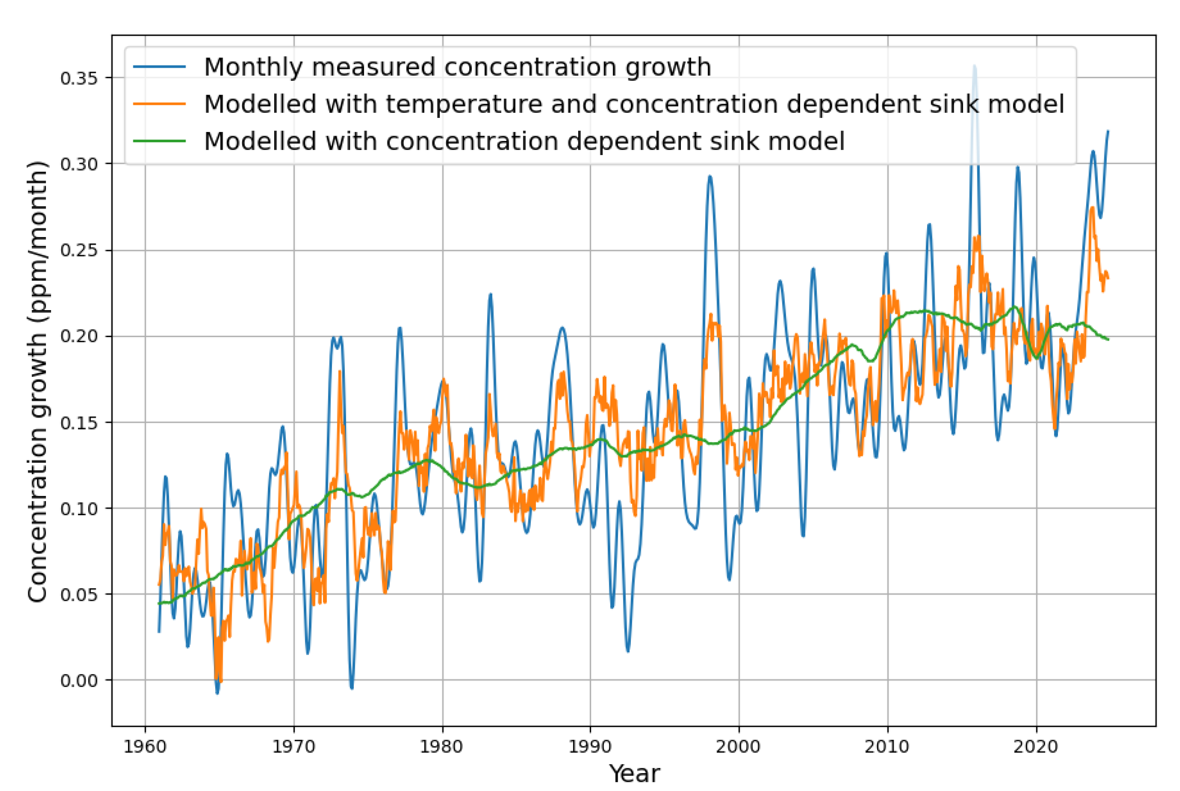
The monthly concentration growth is also reconstructed by the two models. Even in the monthly resolution, the temperature model matches very well the variability of the measured data. There is one noteworthy exception. After 1990, there is a remarkable drop in concentration growth, which has hardly any correspondence in the model variability caused by temperature. The reason has been described by Roy Spences [4], who writes, "Significant model departures from observations occurred for three years after the 1991 eruption of Mt. Pinatubo" and explains it as a consequence of increased photosynthesis due to more diffuse solar radiation.
4. Conclusions
The continuity equation, together with the observed consistent decrease of the C concentration in the atmosphere after 1963 and the observation of temperature-dependent natural emissions, are powerful tools for evaluating observations.
The primary purpose of this article is to explain the recent rise of concentration growth as a consequence of rising sea surface temperatures instead of a hypothetical unobserved decline of absorption by oceans or plants. While the rise of concentration growth is real, the cause is not a failure of sinks but a larger rise of temperature beyond the trend that corresponded to CO level rise.
It should therefore not be off limits to consider temperature as a “normal” cause of CO concentration changes in the public debate, as an influencing factor instead of making wild speculations about the absence of sinks without evidence.
This does not exclude a causality in the other direction; the greenhouse effect, the rather large temperature coefficient on natural CO emissions, certainly limits the possible climate sensitivity.
The most important contribution is that it became possible to separate downwelling absorptions from upwelling natural emissions. Through the evaluation of the bomb test C time series and by the Suess effect correction, we have a reliable estimate of the yearly absorption rate as 4.7% of the CO concentration. Together with the precise CO concentration measurements on Mauna Loa and the accepted measurements of anthropogenic emissions from the International Energy Agency (IEA), the continuity Equation (1) constrains the yearly net natural emissions. Together with the extended model, we also have an understanding of their temperature dependency.
There are other misunderstandings and misconceptions that are challenged by the discussed concepts.
- The most obvious is the argument of some climate skeptics that anthropogenic emissions have no effect because they are apparently "drowned" in the huge natural carbon cycle. The Fact is that anthropogenic emissions are a direct cause of concentration growth. Nature behaves as a strict net sink. This is obvious from Figure 4. Both models end up with a significant, consistent net sink effect for the last 70 years when reliable data were available. Therefore, anthropogenic emissions must have significantly contributed to the total concentration growth.
- Land use change emissions have been an issue for a long time. By interpreting the usually published land use change emissions as anthropogenic, the assumed equilibrium concentration is forced to a value far below the accepted value of 280 ppm. In [8] by only taking half of the published land use change emissions, the equilibrium concentration dropped to an unrealistic 242 ppm. By allowing the land use change emissions to become "natural emissions" and by implication to be small and constant over the last 65 years, not only the prediction quality of the simple model improves, but the equilibrium moves close to 280 ppm [7]. This is not denying them, but looking at them from the correct perspective of the complete carbon cycle.
- Natural emissions by gardens, animals, and even agriculture in general are increasingly becoming a political target. As discussed, increasing natural emissions of the biological sphere are almost always a secondary consequence of a previous increase of photosynthesis and therefore NPP. Therefore, extreme care has to be taken not to create more harm than good by political interference. Mechanical agriculture and chemical contributions to agriculture are already accounted for by the measured anthropogenic emissions. It is therefore not legitimate to count them twice by attaching their effect to the biological product.
- The necessary time shift, where temperature change precedes changes in concentration change, is a clear statement of causality, that to a certain degree CO concentration change follows temperature. As said before, this does not rule out the greenhouse effect, which would be a causality in the other direction.
Of course, questions for further research remain. Due to the fact that the continuity equation must hold at all time scales, we expect new insights about the carbon cycle from systematically changing the timescale and investigating the model parameters.
Funding
This research received no external funding.
Data Availability Statement
All evaluations are based on publicly available data and software: Sea surface temperature data (yearly): https://www.metoffice.gov.uk/hadobs/hadsst4/data/download.html, CO concentration Maona Loa: ftp://aftp.cmdl.noaa.gov/products/trends/co2/co2_mm_mlo.txt, CO emissions, concentration, concentration growth, land use change: https://www.globalcarbonproject.org/carbonbudget/, https://www.icos-cp.eu/science-and-impact/global-carbon-budget/2022. Software: https://www.anaconda.com/ products/distribution, Python modules matplotlib, pandas, statsmodels.
Acknowledgments
Ferdinand Engelbeen has given helpful critical comments on an early version of the manuscript, and pointed to the study of Takahashi et al. about temperature dependence of ocean emissions. Reflecting the issues he raised helped a lot to deepen the understanding and clarifying some formulations. I want to thank Fritz Vahrenholt for the intensive discussions about the relevance of the temperature term. Rolf Dübal gave valuable formal hints that helped to improve the quality of the manuscript.
Conflicts of Interest
The author declares no conflicts of interest.
Abbreviations
The following abbreviations are used in this manuscript:
| NPP | Net Primary Production |
References
- Greenfield, P. Trees and land absorbed almost no CO2 last year. Is nature’s carbon sink failing? https://www.theguardian.com/environment/2024/oct/14/nature-carbon-sink-collapse-global-heating-models-emissions-targets-evidence-aoe, 2024.
- Friedlingstein, P.; O’Sullivan, M.; Jones, M.W.; Andrew, R.M.; Gregor, L.; Hauck, J.; Le Quéré, C.; Luijkx, I.T.; Olsen, A.; Peters, G.P.; et al. Global Carbon Budget 2022. Earth System Science Data 2022, 14, 4811–4900. [Google Scholar] [CrossRef]
- Ke, P.; Ciais, P.; Sitch, S.; Li, W.; Bastos, A.; Liu, Z.; Xu, Y.; Gui, X.; Bian, J.; Goll, D.S.; et al. Low latency carbon budget analysis reveals a large decline of the land carbon sink in 2023. National Science Review 2024, 11, nwae367. [Google Scholar] [CrossRef] [PubMed]
- Spencer, R.W. ENSO Impact on the Declining CO2 Sink Rate. J Mari Scie Res Ocean 2023, 6, 163–170. [Google Scholar] [CrossRef]
- Engelbeen, F.; Hannon, R.; Burton, D. The Human Contribution to Atmospheric Carbon Dioxide. https://co2coalition.org/wp-content/uploads/2024/12/Human-Contribution-to-Atmospheric-CO2-digital-compressed.pdf, 2024.
- Engelbeen, F. The origin of the increase of CO2 in the atmosphere. http://www.ferdinand-engelbeen.be/klimaat/co2_origin.html, 2022.
- Dengler, J. Improvements and Extension of the Linear Carbon Sink Model. Atmosphere 2024, 15. [Google Scholar] [CrossRef]
- Dengler, J.; Reid, J. Emissions and CO2 Concentration—An Evidence Based Approach. MDPI Atmosphere 2023, 14, 566. [Google Scholar] [CrossRef]
- Brownlee, J. How to Identify and Remove Seasonality from Time Series Data with Python. https://machinelearningmastery.com/time-series-seasonality-with-python/, 2020.
- Dietze, P. Carbon Model Calculations. https://www.john-daly.com/dietze/cmodcalc.htm, 2001.
- Halparin, A. Simple Equation of Multi-Decadal Atmospheric Carbon Concentration Change. https://defyccc.com/docs/se/MDACC-Halperin.pdf, 2015.
- Dübal, H.; Vahrenholt, F. Oceans’ surface pH-value as an example of a reversible natural response to an anthropogenic perturbation. Ann Mar Sci 2023, 7, 034–039. [Google Scholar] [CrossRef]
- Vollmer, M.; Eberhardt, W. A simple model for the prediction of CO2 concentrations in the atmosphere, depending on global CO2 emissions. European Journal of Physics 2024, 45, 025803. [Google Scholar] [CrossRef]
- Seabold, S.; Perktold, J. statsmodels: Econometric and statistical modeling with python. In Proceedings of the 9th Python in Science Conference; 2010. [Google Scholar]
- Meacham-Hensold, K. The difference between C3 and C4 plants. https://ripe.illinois.edu/blog/difference-between-c3-and-c4-plants, 2020.
- Haverd, V.; Smith, B.; Canadell, J.G.; Cuntz, M.; Mikaloff-Fletcher, S.; Farquhar, G.; Woodgate, W.; Briggs, P.R.; Trudinger, C.M. Higher than expected CO2 fertilization inferred from leaf to global observations. Global Change Biology 2020, 26, 2390–2402. [Google Scholar] [CrossRef]
- Humlum, O.; Stordahl, K.; Solheim, J.E. The phase relation between atmospheric carbon dioxide and global temperature. Global and Planetary Change 2013, 100, 51–69. [Google Scholar] [CrossRef]
- Richardson, M. Comment on "The phase relation between atmospheric carbon dioxide and global temperature" by Humlum, Stordahl and Solheim. Global and Planetary Change 2013, 107, 226–228. [Google Scholar] [CrossRef]
- Hua, Q.; Turnbull, J.C.; Santos, G.M.; Rakowski, A.Z.; Ancapichun, S.; De Pol-Holz, R.; Hammer, S.; Lehman, S.J.; Levin, I.; Miller, J.B.; et al. ATMOSPHERIC RADIOCARBON FOR THE PERIOD 1950-2019. Radiocarbon 2022, 64, 723–745. [Google Scholar] [CrossRef]
- Suess, H.E. Radiocarbon Concentration in Modern Wood. Science 1955, 122, 415–417. [Google Scholar] [CrossRef]
- Levin, I.; Kromer, B.; Schoch-Fischer, H.; Bruns, M.; Münnich, M.; Berdau, D.; Vogel, J.C.; Münnich, K.O. 25 Years of Tropospheric 14C Observations in Central Europe. Radiocarbon 1985, 27, 1–19. [Google Scholar] [CrossRef]
- Stuiver, M.; Polach, H.A. Discussion Reporting of 14C Data. Radiocarbon 1977, 19, 355–363. [Google Scholar] [CrossRef]
- Stuiver, M.; Quay, P. Atmospheric14C changes resulting from fossil fuel CO2 release and cosmic ray flux variability. Earth and Planetary Science Letters 1981, 53, 349–362. [Google Scholar] [CrossRef]
- Burton, D.A. Comment on Stallinga, P. ( Residence Time vs. Adjustment Time of Carbon Dioxide in the Atmosphere, 2024. [CrossRef]
- Graven, H.; Keeling, R.F.; Rogelj, J. Changes to Carbon Isotopes in Atmospheric CO2 Over the Industrial Era and Into the Future. Global Biogeochemical Cycles 2020, 34, e2019GB006170. [Google Scholar] [CrossRef]
- Nemani, R.R.; Keeling, C.D.; Hashimoto, H.; Jolly, W.M.; Piper, S.C.; Tucker, C.J.; Myneni, R.B.; Running, S.W. Climate-Driven Increases in Global Terrestrial Net Primary Production from 1982 to 1999. Science 2003, 300, 1560–1563. [Google Scholar] [CrossRef]
- Zhao, M.; Running, S.W. Drought-Induced Reduction in Global Terrestrial Net Primary Production from 2000 Through 2009. Science 2010, 329, 940–943. [Google Scholar] [CrossRef]
- Bond-Lamberty, B.; Thomson, A. Temperature-associated increases in the global soil respiration record. Nature 2010, 464, 579–582. [Google Scholar] [CrossRef]
- Hashimoto, S.; Carvalhais, N.; Ito, A.; Migliavacca, M.; Nishina, K.; Reichstein, M. Global spatiotemporal distribution of soil respiration modeled using a global database. Biogeosciences 2015, 12, 4121–4132. [Google Scholar] [CrossRef]
- Davidson, E.A.; Janssens, I.A. Temperature sensitivity of soil carbon decomposition and feedbacks to climate change. Nature 2006, 440, 165–173. [Google Scholar] [CrossRef] [PubMed]
- Takahashi, T.; Olafsson, J.; Goddard, J.G.; Chipman, D.W.; Sutherland, S.C. Seasonal variation of CO2 and nutrients in the high-latitude surface oceans: A comparative study. Global Biogeochemical Cycles 1993, 7, 843–878. [Google Scholar] [CrossRef]
- Hunter, J.D. Matplotlib: A 2D graphics environment. Computing in Science & Engineering 2007, 9, 90–95. [Google Scholar] [CrossRef]
- NOAA. Trends in Atmospheric Carbon Dioxide (CO2), 2023, [https://gml.noaa.gov/ccgg/trends/data.html].
- Kennedy, J.J.; Rayner, N.A.; Atkinson, C.P.; Killick, R.E. An ensemble data set of sea-surface temperature change from 1850: the Met Office1 Hadley Centre HadSST.4.0.0.0 data set. Journal of Geophysical Research Atmospheres 2019, 124. [Google Scholar] [CrossRef]
Figure 1.
Monthly Maona Loa time series of CO concentration and deseasonalized monthly CO concentration data.
Figure 1.
Monthly Maona Loa time series of CO concentration and deseasonalized monthly CO concentration data.
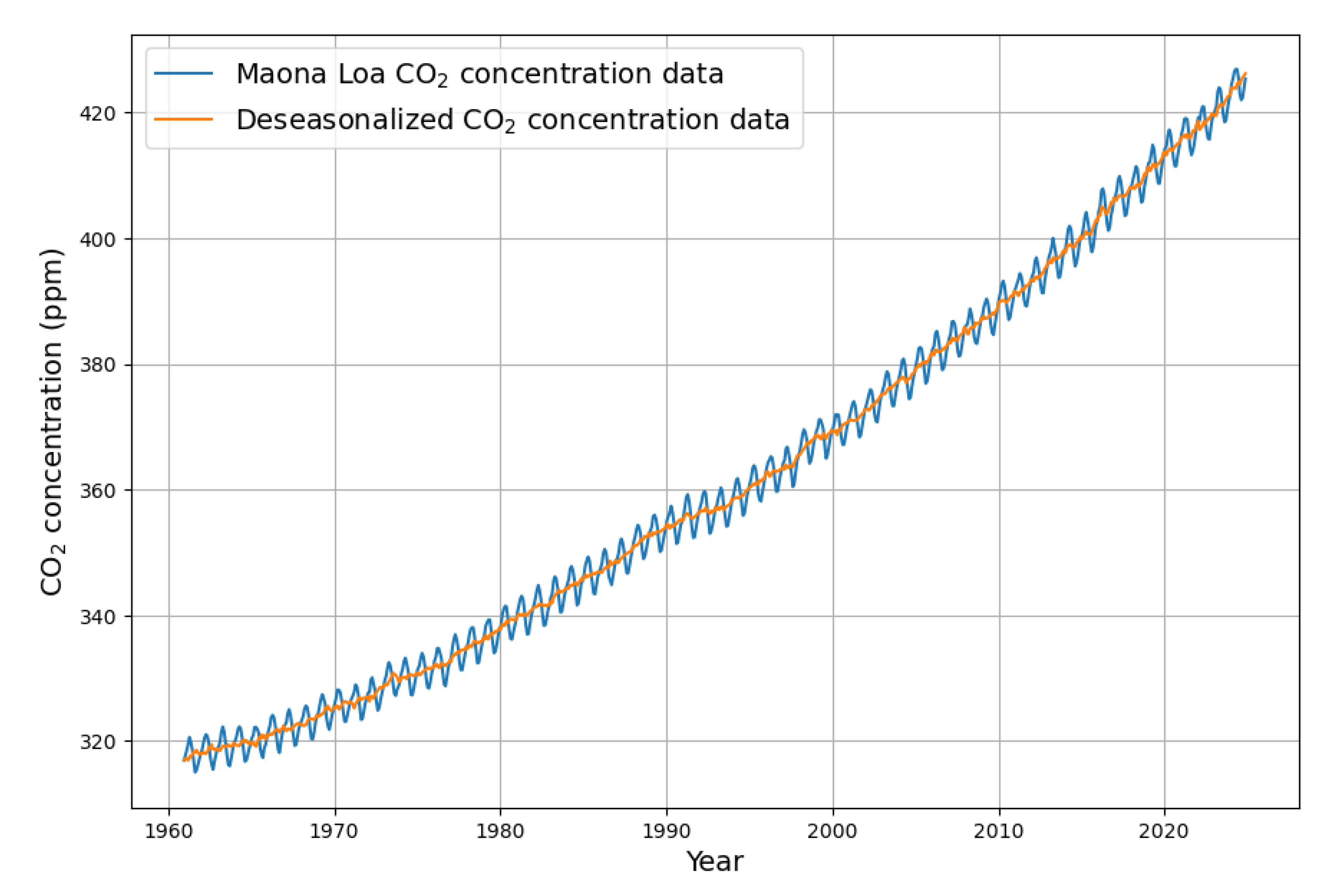
Figure 2.
Monthly global sea surface temperature time series and deseasonalized monthly global sea surface temperature data.
Figure 2.
Monthly global sea surface temperature time series and deseasonalized monthly global sea surface temperature data.
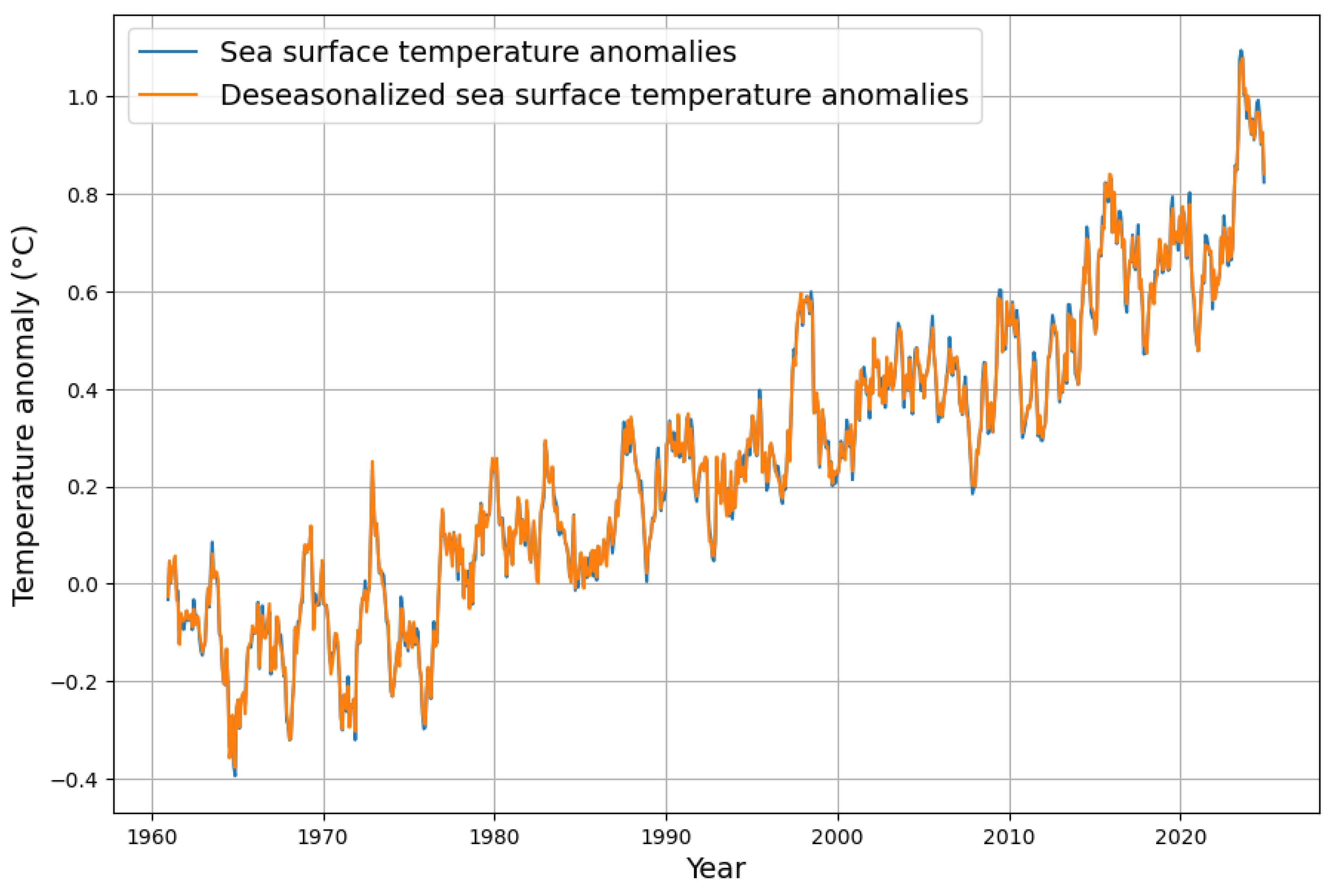
Figure 3.
Monthly deseasonalized concentration growth.
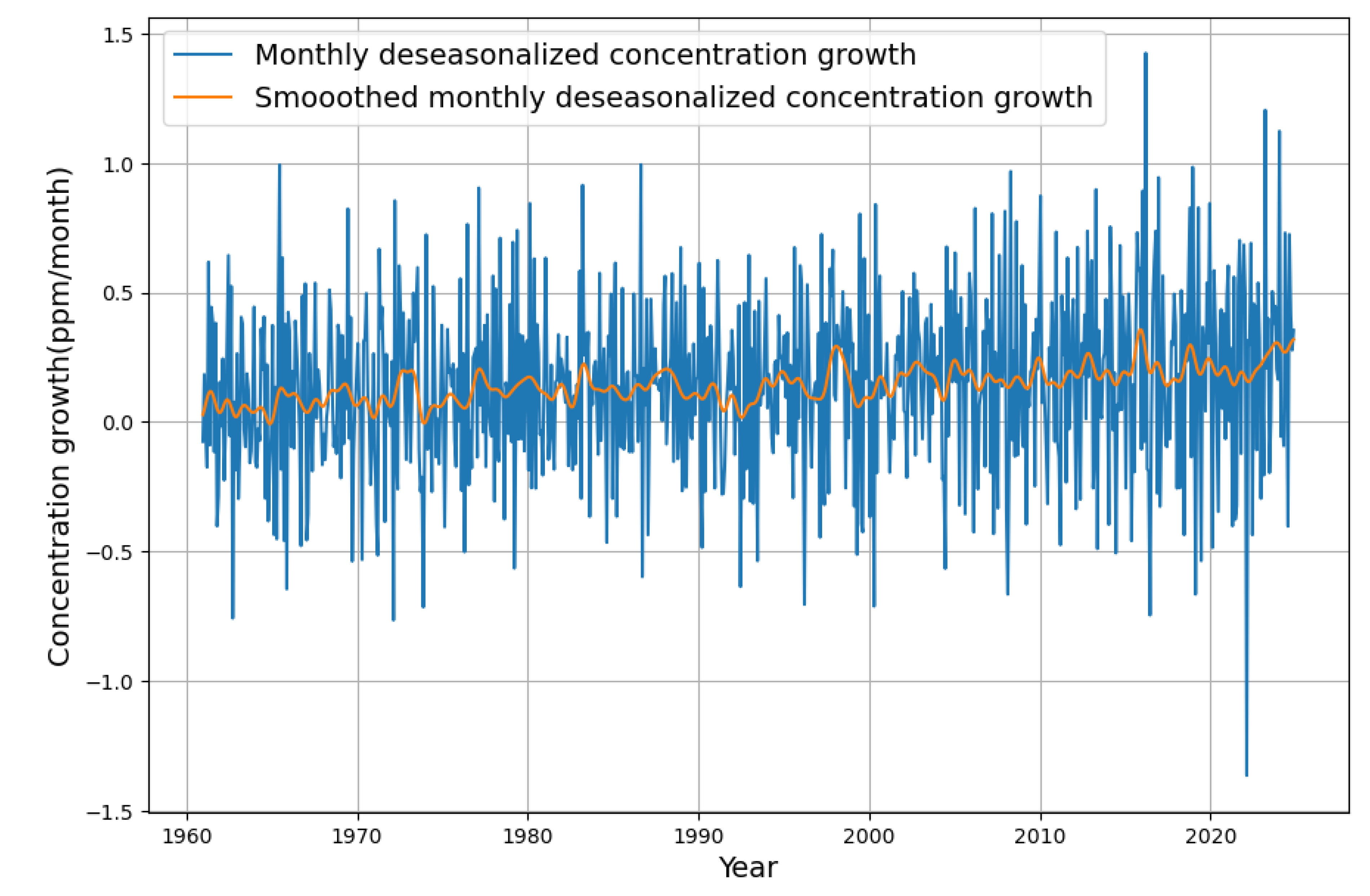
Figure 4.
Anthropogenic emissions (blue), CO concentration growth (orange)and sink effect (green).
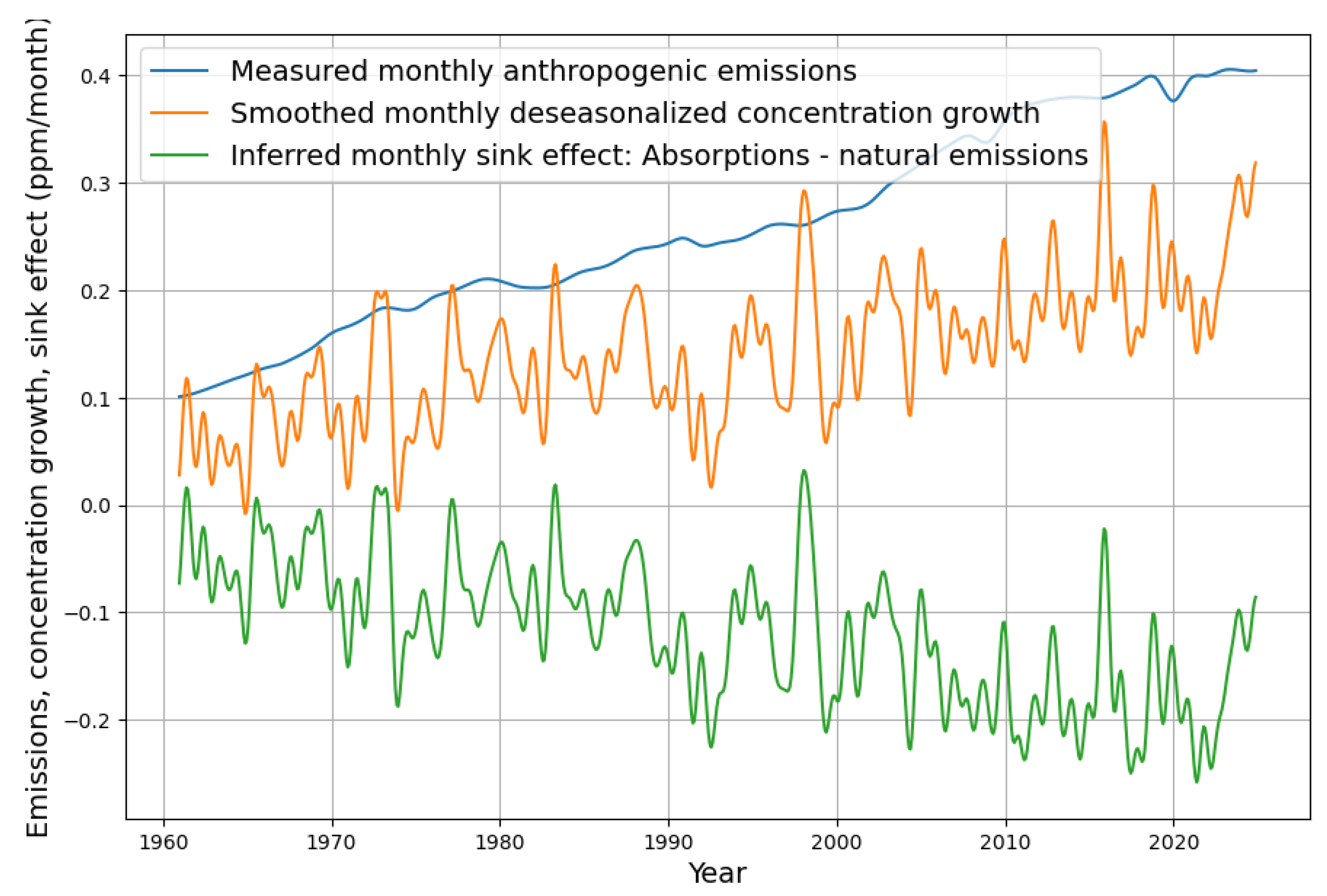
Figure 5.
Sea surface temperature, original (blue) temperature modelled with CO (orange)
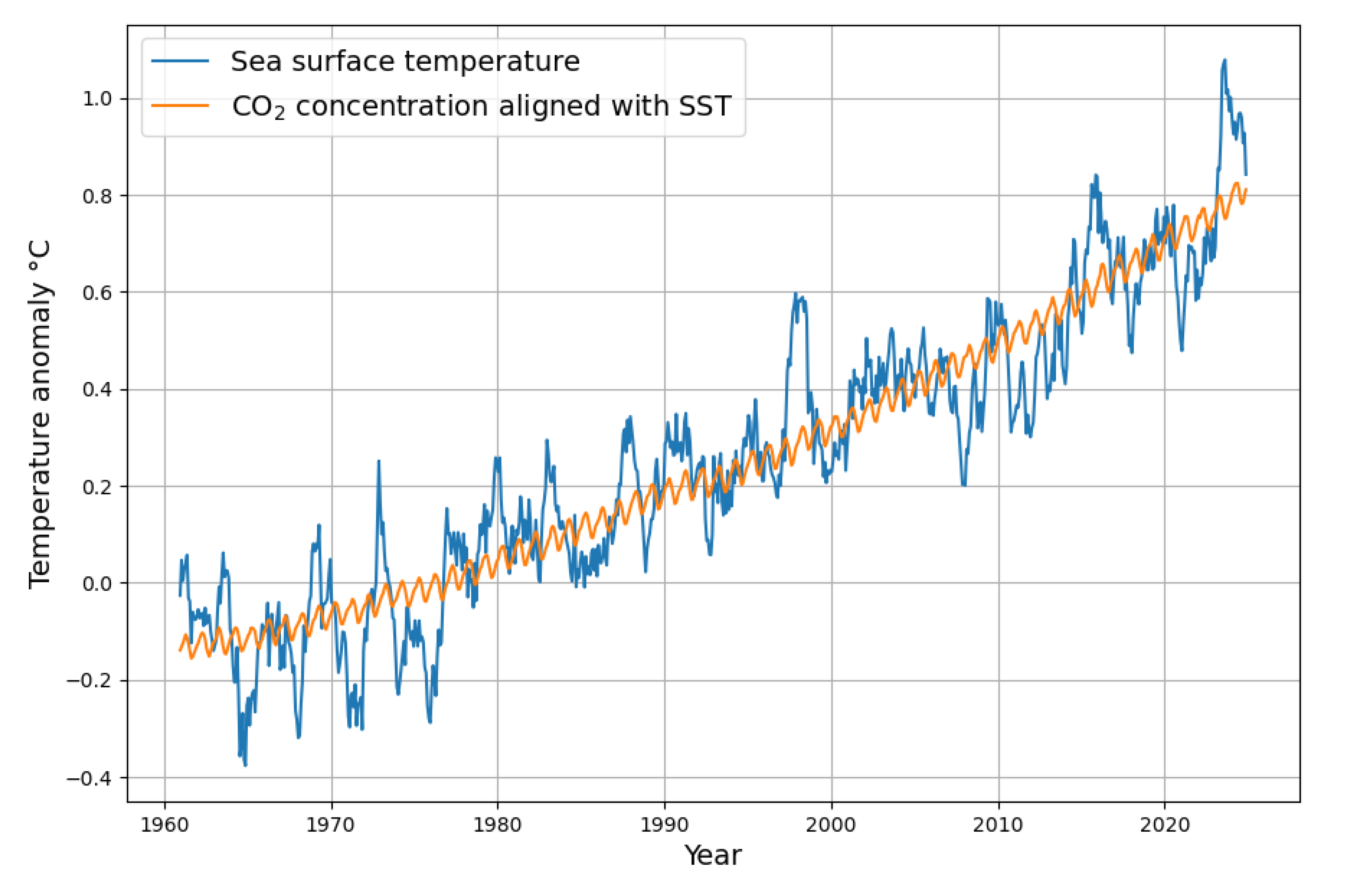
Figure 6.
The decay of the global atmospheric C after 1965. Published data are blue, adjusted data are orange.
Figure 6.
The decay of the global atmospheric C after 1965. Published data are blue, adjusted data are orange.
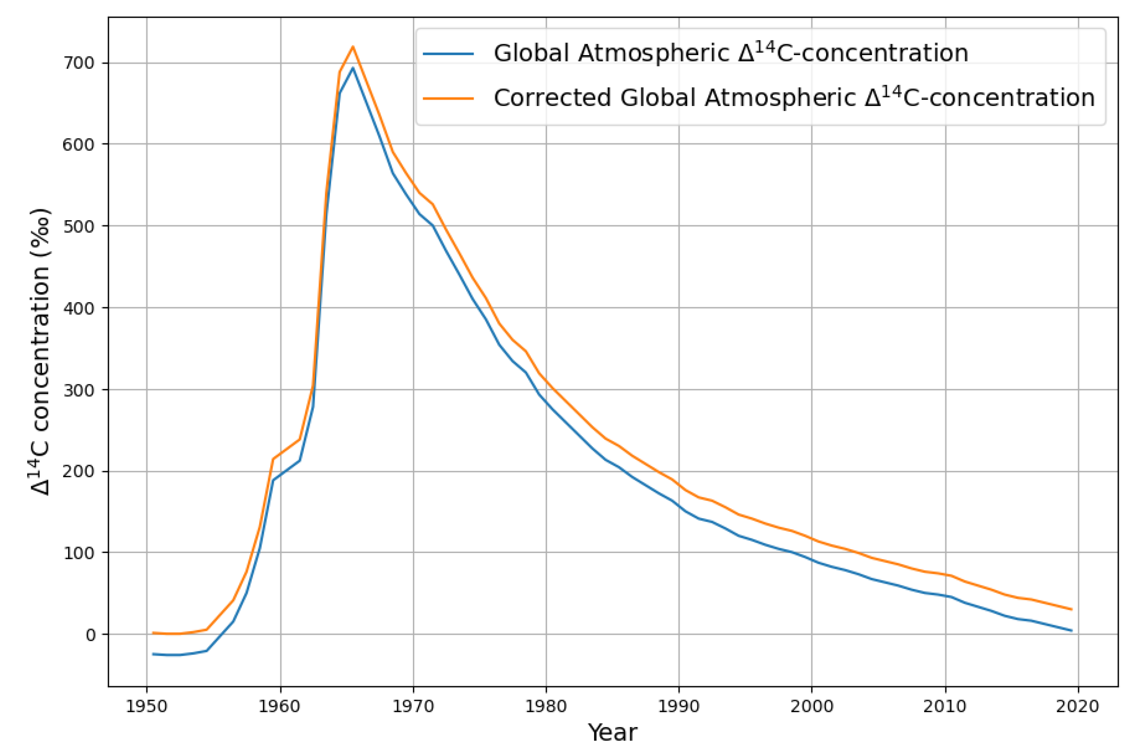
Figure 7.
Determination of the C decay rate by a logarithmic transformation
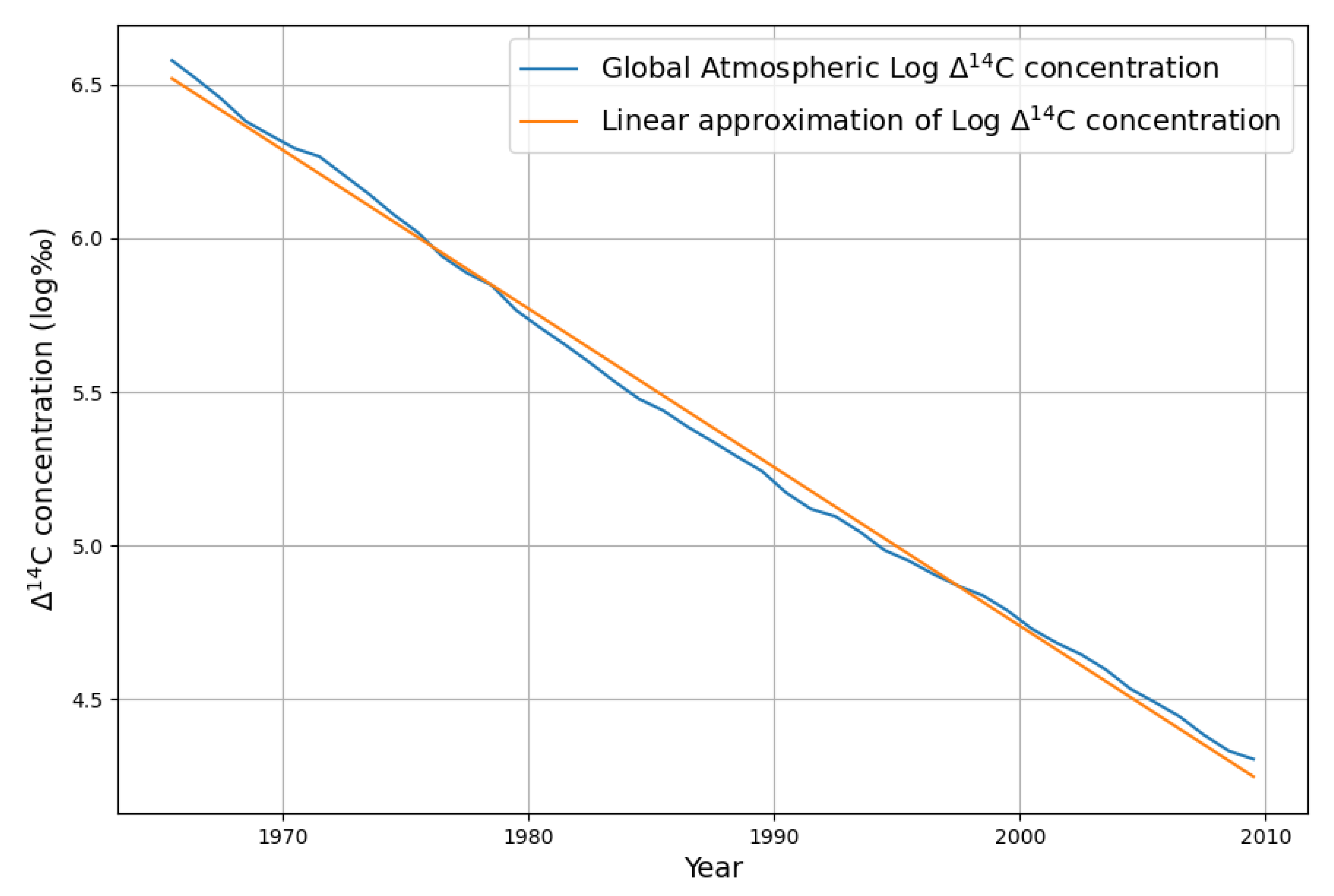
Figure 8.
Explained variance of extended model as a function of temperature shift, measured in months
Figure 8.
Explained variance of extended model as a function of temperature shift, measured in months
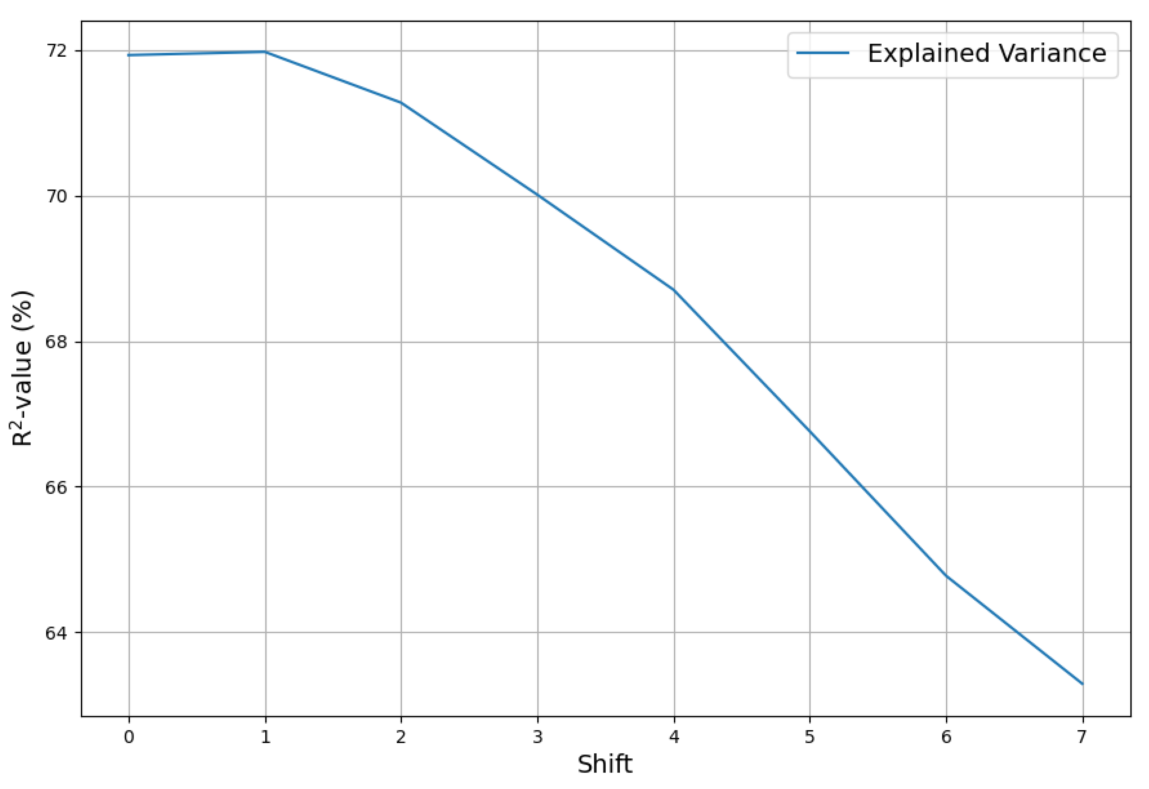
Figure 9.
Composition of the the measured sink effect (red) by absorptions (green) and natural emissions (blue)
Figure 9.
Composition of the the measured sink effect (red) by absorptions (green) and natural emissions (blue)
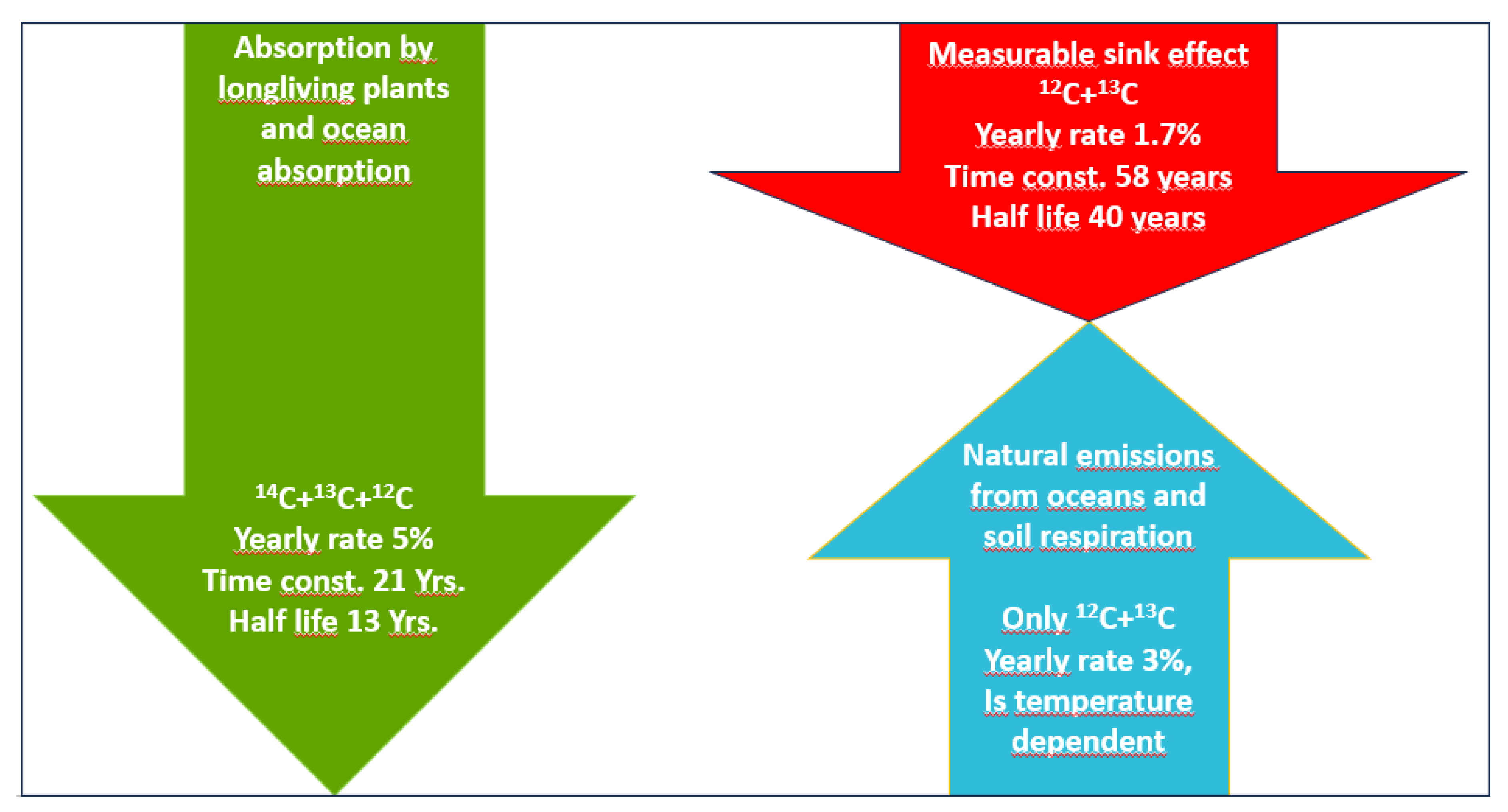
Figure 10.
Yearly sink effect (blue), result of simple sink model (green), and result of extended sink model (orange).
Figure 10.
Yearly sink effect (blue), result of simple sink model (green), and result of extended sink model (orange).
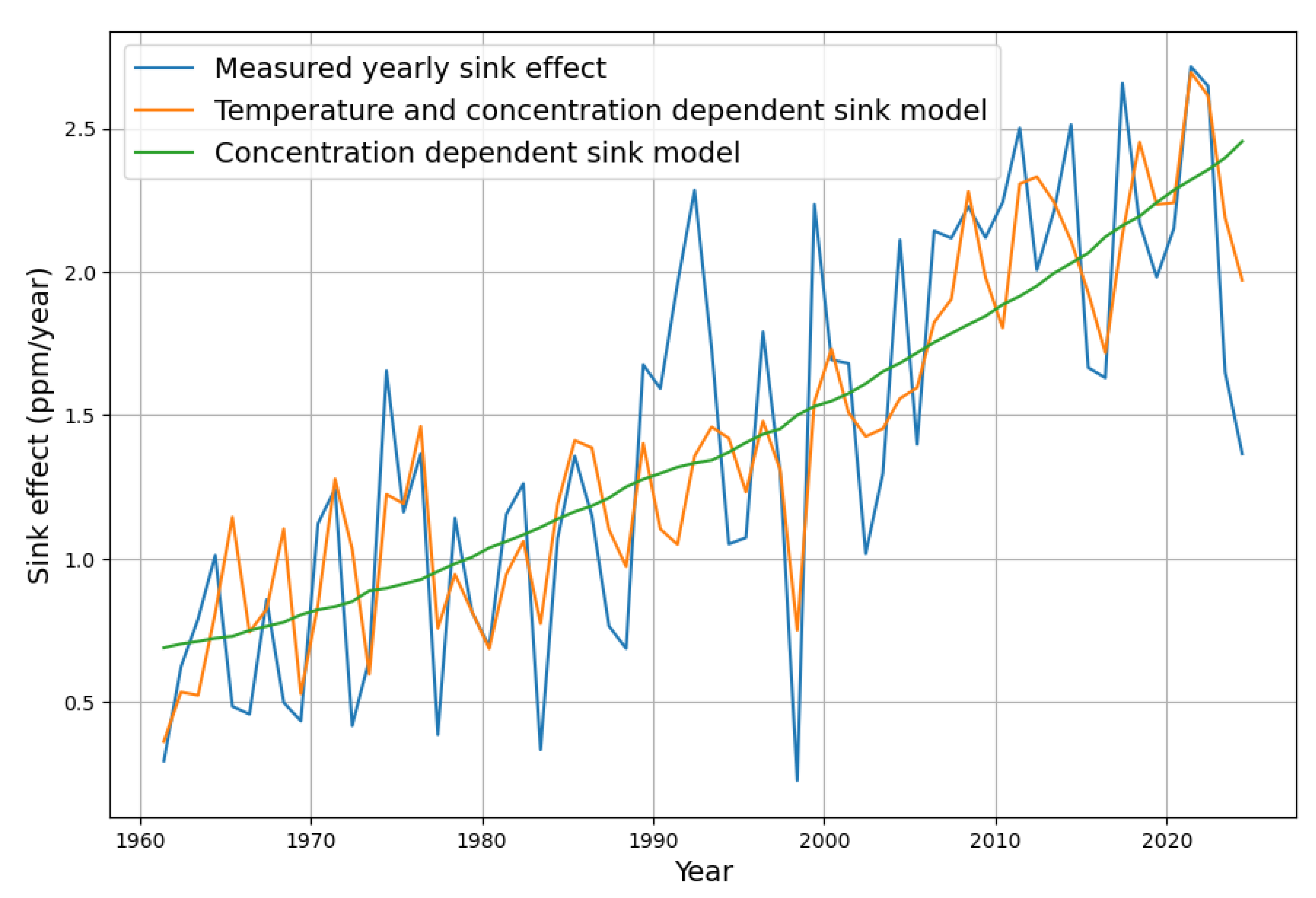
Figure 11.
Yearly concentration growth (blue) and its modeling with simple sink model (green) and temperature-dependent extended sink model (orange).
Figure 11.
Yearly concentration growth (blue) and its modeling with simple sink model (green) and temperature-dependent extended sink model (orange).
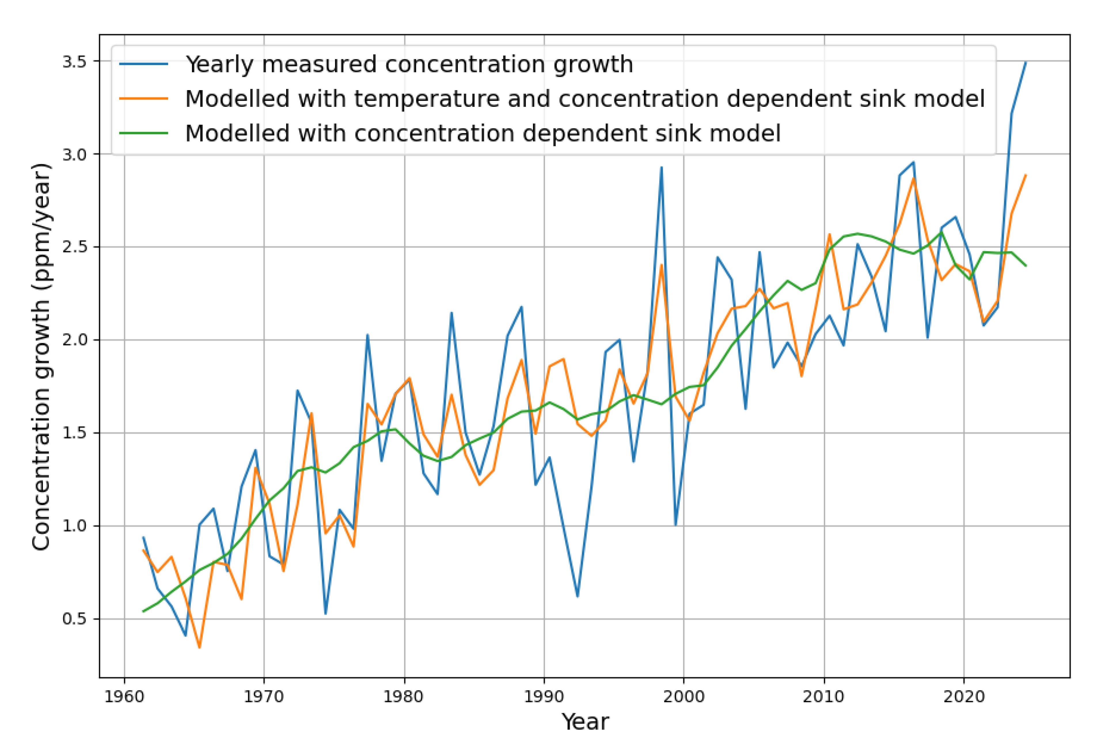
Figure 12.
Monthly concentration growth (blue) and its modeling with simple sink model (green) and temperature-dependent extended sink model (orange).
Figure 12.
Monthly concentration growth (blue) and its modeling with simple sink model (green) and temperature-dependent extended sink model (orange).
Disclaimer/Publisher’s Note: The statements, opinions and data contained in all publications are solely those of the individual author(s) and contributor(s) and not of MDPI and/or the editor(s). MDPI and/or the editor(s) disclaim responsibility for any injury to people or property resulting from any ideas, methods, instructions or products referred to in the content. |
© 2025 by the authors. Licensee MDPI, Basel, Switzerland. This article is an open access article distributed under the terms and conditions of the Creative Commons Attribution (CC BY) license (http://creativecommons.org/licenses/by/4.0/).
Copyright: This open access article is published under a Creative Commons CC BY 4.0 license, which permit the free download, distribution, and reuse, provided that the author and preprint are cited in any reuse.


