Submitted:
23 April 2025
Posted:
24 April 2025
You are already at the latest version
Abstract
Forecasting systemic financial risks is important to prevent and resolve systemic financial risks effectively. In this paper, we give a method to measure and predict the systemic financial risk of China’s financial industry based on stock trading data of 36 China’s A-share listed financial institutions. We establish a complex financial network and obtain three clusters of the system by spectral clustering. A weighted average value is defined to measure the systemic risk of each cluster. Based on the interrelationship of different clusters, phase space reconstruction and delay parameterization method (RDPM), radial basis function neural network (RBF) are used together to forecast the systemic financial risk. The relative accuracy of prediction is more than 95%, which is higher than that of some common machine learning methods.
Keywords:
systemic financial risk
; forecast
; phase space reconstruction
; delay parameterization method
; machine learning
1. Introduction
Since the outbreak of the US subprime crisis in 2008, there has been a growing intensity in research on the systemic risk of financial markets. The bankruptcy of Lehman Brothers and the European debt crisis have exposed vulnerabilities within the financial system. A large-scale financial crisis not only infilicts significant harm on economic operations but also highlights the lack of effective mechanisms to address such events and risks [1]. While financial regulators cannot entirely prevent crises from occurring, early detection of warning signals can assist in formulating effective macro policies. Consequently, with the integration and increasing complexity of financial markets, predicting systemic financial risks has become an urgent and challenging task within financial research [2]. In recent years, numerous research findings on systemic financial risks have emerged, primarily focusing on measuring these risks, understanding contagion and spillover effects, identifying influencing factors, as well as exploring their interaction with macroeconomic conditions [[3[6].
Benoit believes that systemic risk impacts multiple market participants at the same time, and will further spread throughout the entire financial system [7]. It has been widely recognized that systemic risk has a fast contagion speed and wide impact, and will lead to currency depreciation, market downturn, and recession of a country or even the world economy [8]. Systemic risk is often considered difficult to define. Summer believes that the difficulty lies in the lack of a general theoretical framework that can strictly distinguish between the crisis contagion itself and the joint crisis caused by the common impact [9]. Accurate measurement of systemic financial risk or the design of relevant proxy indicators are the basis for empirical research. The connectivity of financial markets and the infectivity of risks have eliminated the VaR index [10], and the marginal expected loss (MES) and conditional value at risk (CoVaR), which focus on the overall measurement of financial risks, have been widely used [11,12].
Due to the high correlation between financial markets, complex network theory has been widely applied to the contagion analysis of financial risks. Complex network breaks through the limitation of relationship and examines risk spillover and spread from the perspective of overall correlation [13]. Considering the complexity of the network model, most scholars establish low-dimensional models which including fewer financial entities and resulting in certain biases in relevant studies [14]. In recent years, many scholars have tried to study high-dimensional networks [15,16]. Some scholars choose cluster analysis and other methods to reduce the network dimension and effectively identify the homogeneity of complex systems such as [1][20].
Since there is no effective monitoring mechanism, forward-looking prediction of systemic risk is an important means of supervision. The prediction of the future fluctuation trend of systemic risks and the detection of structural mutation points will help to formulate macro policies and take preventive measures in advance [21].
Systemic risk is measured by high-frequency data of the financial market, so it inherits the characteristics of nonlinearity, high noise and chaos of financial time series [22]. Traditional measurement models, such as ARIMA model, based on the premise of linear assumption, cannot effectively predict the volatility of systemic risk [23]. In recent years, machine learning, such as support vector machine, random forest, neural network and deep learning have achieved good forecasting effect in the financial field [2][27]. However, the “blackbox” nature of machine learning also makes predictions much less interpretable.
Meanwhile, many nonlinear tools, such as differential equations [28,29] and phase space reconstruction [30,31] are used to study financial problems. Phase space reconstruction is a nonlinear dynamic analysis tool derived from chaos theory. By mapping one-dimensional financial time series to multidimensional space, it is expected to capture the nonlinear relationship and dynamic evolution process of financial system in a more comprehensive way [32]. Stochastic distribution embedding based on phase space reconstruction has good performance in predicting short- term high-dimensional data [33,34]. In [35], the time-varying point detection has been successfully carried out, and the abnormal fluctuations caused by the bankruptcy of Lehman Brothers Bank before the subprime crisis has been successfully verified. The delayed parameterization method (DPM) shows good characteristics in predicting stock market prices and indexes [30,34].
The increasing complexity of financial market brings new challenges to the accuracy of prediction. Many scholars use combination methods to extract effective information of financial time series in order to improve the accuracy of prediction. The features of time series are extracted by phase space reconstruction technology as the input of Net model. Reference [29] combines the advantages of neural network and stochastic differential equation to achieve high-quality prediction of stock index.
In the future, risk management and analysis in the financial field will be driven by artificial intelligence and big data [3][39]. The combination of cross-domain research methods is expected to solve more efficiently the complex problems of the financial system.
In this paper, we measure and predict the systemic financial risk of China’s financial industry based on stock trading data of 36 China’s A-share listed financial institutions. Firstly, we establish a complex financial network and obtain three subsystems by spectral clustering, then use a weighted average value to measure the systemic financial risk of every cluster. Secondly, we predict the systemic financial risk by combination of phase space reconstruction, delay parameterization method and radial basis function neural network. The relative accuracy of prediction is more than 95%, and the prediction effect is better than that of a single common neural network method. Finally, based on the predicted results, the time points of the Sino-US trade war and the large-scale outbreak of the COVID-19 are tested, which are the points that systemic financial risk. To the best of our knowledge, this is the first paper that phase space reconstruction theory has been applied to the prediction of systemic financial risk.
The rest of this paper are arranged as follows: we introduce phase space reconstruction method in section 2. The section 3 is devoted to the measurement of systemic risk. The forecast process and results of systemic risk are presented in Section 4. In section 5, according to the prediction results, we detect the abnormal points of the systemic risk series, and find the mutation time points of the Sino-US trade war and the large-scale outbreak of COVID-19. In Section 6, we give a summary of the main conclusion of this paper.
2. Phase Space Reconstruction and Delay Parameterization Method (RDPM)
The prediction principle of phase space reconstruction method is derived from Takens’ embedding theorem and generalized embedding theorem [40,41]. According to two embedding theorems, the trajectory information in the reconstructed phase space is topologically equivalent to the dynamical evolution of the original system. Hence, it can be applied to establish the prediction model. For better understanding, suppose the original observation data is vector set, and the phase space composed of original multiple observations is
where m is the number of vector and N is the data length. The phase space reconstructed by kth observation function is
Here, the embedding dimension of the phase space d = m for simplicity, and is the delay parameter, both Y and are m-dimension spaces. Suppose be a linear function such that
Here, P is the parameter matrix constituted by the coefficients of coupling relation between Y and . The unknown data in are and Note that the first lines of are known. We defined the first line of and Y as new matrixes and , that is,
then the parameter matrix P can be solved by the equation .
According to , we can obtain the prediction of the sequence However, the linear mapping P can hardly reflect the complex mapping relationship between financial time series. Hence, in the following paper, we use radial basis function (RBF) neural network to train the mapping relationship.
There are many methods to determine the time delay, such as autocorrelation function method, mutual information method [42,43] etc. In order to make full use of the internal dynamic evolution information of the system, we consider the time delay
uniformly. Referring to literatures [30,31], we adopt the delay parameterization method to find optimal time delay and minimize the overall training prediction error of the system. Define an object function
where represents the predicted value and represents the true value, and are the mean value and standard deviation. The optimal time delay minimizes the object function f in (4). A brief description of the method is given here, readers can refer to [30] for a detailed discussion.
Let . The observation seriesis divided into training set and test set. belong to training set and
belong to test set. Here, need to be predicted.
The prediction is carried out according to the following steps:
- Step1
- Observe and normalization the variable
still denoted by for convenience;
- Step2
- For
- The normalized matrix are constructed;
- Train the network with as the input matrix and as the output matrix;
- Using the test matrix as a new input matrix and the network structure obtained in 2, predict
Compute the object function f ;
end for
- 4.
- Minimize the object function f and choose the optimal delay ;
- Step3: Single-step prediction
- The matrix and are reconstructed by using normalized and the optimal delay ;
- Train the network with as the input matrix and as the output matrix, where ;
- Using the network structure obtained in 2 and the test matrix as new input and predicts ;
- Add the predicted value
to the observed variable;
end
- Step4 Obtain the predicted value . Then inverse normalization. Process is performed;
- Step5: Calculate MAE, MSE and RMSE. Three indexes to evaluate the prediction effect are mean absolute error (MAE), mean square error (MSE) and root mean square error (RMSE):
3. Measurement of Systemic Financial Risk
3.1. Data
We select the financial institutions which were listed in the China A-share before July 1, 2015 as research object. A total of 40 listed enterprises include banking, securities, insurance and trust. Excluding those with serious missing annual data and marked with ST, 36 listed financial institutions are selected as effectively sampled (see Appendix A), including 15 banks, 15 securities companies, 4 insurance companies and 2 trust companies. The market value of the sample institutions accounted for 77.3% of the total market value of A-share listed financial institutions in 2022. We choose the daily closing prices of 36 institutions from July 1, 2015 to December 30, 2020, total 1342 trading days data. Date comes from the CSMAR database. The tail processing is carried out according to 1% above or below to eliminate the influence of outliers. The sample interval includes the stock market volatility in 2015, the stock market circuit breaker in 2016, the Sino-US trade war in 2018 and covers the time before and after the outbreak of COVID-19 pandemic.
3.2. Measurement of Systemic Financial Risk
The most commonly measure for assessing the risk of an individual financial institution is value-at-risk (VaR). The maximum loss of the institution i at time t at the confidence level (e.g., 95%) is defined as:
where is the return rate of the institution i at time t and is the closing price of stock i in period t. The represents the maximum loss of financial institution i under normal conditions, and represents the loss of institution i when the risk occurs.
To measure the contribution of each institutional asset to systemic risk, Adrian and Brunnermeier [44] proposed the concept of conditional value-at-risk (CoVaR), defined as follows:
Here is the return rate of the market, and represents the conditional risk to which the system is exposed when the financial institution i has suffered an extreme loss at time t. We employ quantile regression techniques to estimate CoVaR. The selected state variables are the volatility of CSI 300 index and the growth rate of CSI 300 index*, which are used to measure the volatility of the stock market.
The spillover of risk from institution i to the financial system s can be measured in terms of:
The confidence level is set to 95%, that is, . has proven to be a valuable tool for assessing systemic risk in financial markets [12].
In this paper, the value of we obtain are all negative. To simplify the analysis, we use absolute values to measure the systemic risk. The larger the value, the greater the individual institution’s contribution to systemic risk.
Figure 1 shows the sequence of of Guotai Junan (securities), Agricultural Bank of China (bank) and China Pacific Insurance (insurance). As can be seen from Figure 1, the sequences have strong irregular volatility.
Table 1 shows the daily average of each financial institution during the sample period. The securities and insurance companies dominate the top 10. Although the number of insurance companies is small, accounting for only 12% of the total number of samples, Ping An of China, New China Insurance and China Pacific Insurance ranked 6th, 7th and 10th respectively. The contribution of some securities companies to the systemic risk is higher. The contribution of most banks to financial risk is at a moderate level.
Table 2 lists the average values of of different industries. The insurance industry has the highest systemic risk, followed by the securities industry and the bank. Specially, the average value of of the insurance industry is much higher than that of the bank. This shows that the insurance industry is an important source of systemic risk. The banking industry is relatively stable in China’s financial system.
3.3. Construction of Complex Network Model of Financial System
Complex network model has proved to be an effective tool to study the interconnectedness of financial system. By building complex networks, we can better analyze the internal structure and connectivity of the financial system. In order to examine the risk of the financial system, this paper constructs a complex network with 36 financial institutions as nodes:
(1) Nodes: The network nodes are the 36 A-share listed financial institutions listed in Appendix A.
(2) Edge: We establish the edge through the correlation between stocks [10]. The correlation coefficient of the sequence and is calculated:
where is the logarithmic return rate of stock i at time t.
For simplifying the network, we chose a certain threshold for . If , we consider that there is an edge between stock i and j. Otherwise there is no edge. The selection of threshold will affect the specific structure of the network. According to the research conclusion of Bo Zheng et al. [11], the threshold can be calculated as
where N = 36 is the total number of financial institutions. The network is shown in Figure 2.
In Figure 2, most financial institutions are closely related each other. The network diagram presents a “dumbbell” shape. The securities companies are mainly concentrated on the left side, the banks are mainly concentrated on the right side, and the insurance companies are scattered in the middle. The relevant measurement indicators of the network model are shown in Table 3.
The degree of a node represents the number of edges connected between the node and other nodes, and degree centrality represents the ratio of the degree to the maximum number of edges that the node may have, reflecting the importance of node in the network. The distance between two nodes is the number of edges contained in the shortest path connecting them, and the network average pathlength refers to the average distance between two nodes. The network diameter is defined as the maximum distance between two nodes in the network. Network density is the ratio of the actual number of edges in the network to the maximum number of edges that can be accommodated, which reflects the density of the network.
The average degree of the complex network in Figure 2 is 20.72, and the average degree centrality is 0.592. The average path length is 1.443, and the network diameter is 3. The network density is 0.296. These indicate that the network is a relatively dense and the connectivity between nodes is strong. Once the risk occurs, it will spread through the entire system at a faster speed. Table 4 lists the degree centrality of each node.
We find that the top 10 of degree centrality are security and insurance institutions. The mean degree centrality of the securities industry is 0.6857, that of the banking industry is 0.5294, and that of the insurance industry is 0.3809. This difference is mainly due to the large-scale expansion and development of securities companies with the development of national economy and finance, and the formation of close economic relations with the real economy and other financial institutions. Banks have a special position in China’s financial system, especially the four major commercial banks. Although their frequency of connection with other institutions in the financial market are not the highest, but the banks play an important role in maintaining system stability.
3.4. Cluster Analysis
The sequence of 36 financial institutions represents the risk spillover value of individual financial institutions to the financial system. We need to define a proxy indicator for the systemic risk of the financial system. A natural way is to calculate the weighted average of according to the important of nodes in the financial network. However, it is too rough to measure the systemic financial risk.
Generally, financial risks will first spread among closely connected nodes, and then continue to spread and spill over to other nodes. Therefore, we use the clustering method to divide the system into several small clusters. Then, we consider the systemic risks of each cluster and the mutual influence of risks among clusters. By classifying nodes in a complex network, cluster analysis reveals the maximum homogeneity among nodes in the system, which can effectively identify high-risk clusters within the financial system and then discover the risk propagation path. Cluster analysis is widely used in stock index volatility analysis and loan default and other financial risk prevention and control [12,13]. Spectral clustering is an effective tool to reveal the higher-order organization of complex networks, which has been widely used in physics, neuroscience, social science, financial risk analysis and other field [14]. For detailed research and specific algorithms of spectral clustering, please refer to reference [19]. This section performs spectral clustering on a complex network of 36 financial institutions. The clustering results are shown in Figure 3.
The specific financial institutions contained in the three clusters are shown in Table 5. Table 5 shows that in the actual economic operation, the closely connected institutions may come from different industries.
The results obtained by spectral clustering are very different from the traditional classification by industry. In Cluster 1, securities companies account for 50%, among which, Shanxi Securities, Guotai Junan and other securities companies are at a high level of systemic risk. In Cluster 2, banks account for 46%. In particular, systemically important banks such as Bank of China and Agricultural Bank of China gather in cluster 2. Cluster 3 contains those institutions that are less connected to other institutions in the system.
3.5. The Weighted Average Value
We calculate the weighted average value of the three clusters as a measure of systemic risk in financial markets. The higher the degree of node, the stronger the infectivity in the event of a crisis. Therefore, a weight is assigned to each financial institution with , here is the degree of node i and n represents the number of financial institutions contained in each cluster. Figure 4 contains three time series of the daily weighted average value of the three clusters from January 2, 2019 to December 30, 2020 reflecting the dynamic changes of the systemic financial risk value of the three clusters.
On the whole, the risk value of Cluster 1 is slightly higher than that of Cluster 2, because there are more securities institutions distributed in cluster 1, and some securities institutions have higher risks. Cluster 2 contains more banks. The risk value of cluster 3 is significantly lower than that of the other two clusters, and the risk contribution to the system is relatively low. Generally speaking, risks are propagated from institutions with higher risks to institutions with lower risks, and continue to propagate to other institutions after reaching the overflow threshold [13]. Financial risks accumulate in cluster 1, spread to Cluster 2, and finally spread to Cluster 3. Table 6 shows the descriptive statistical characteristics of the systemic financial risks of each cluster. Cluster 1 has a higher mean of 1.226 than the other two subcategories, and Cluster 3 has the lowest mean of 1.034. In addition, the extreme risk of Cluster 1 is much higher than that of the other two subclasses, with a range of 6.204 and a large fluctuation. The fluctuation amplitude of Cluster 2 is the smallest, indicating that the systemic risk of Cluster 2 remains relatively stable.
3.6. Chaotic Identification of Systemic Financial Risk Sequence
Figure 4 shows the daily weighted average of for all three clusters showing jagged irregular fluctuation. Based on the nonlinear and high noise characteristics of financial time series, it is necessary to determine whether the sequences of the three clusters are chaotic. In this section, Lyapunov index is used for judging whether time series has chaos [45,46]. There are many main methods to calculate the Lyapunov index. In this paper, the small data quantity method proposed in [45] is used to calculate the Lyapunov index of time series. This method has some advantages such as reliable results, small computation amount and easy operation, and is suitable for practical problems. The sequence is chaotic if its Lyapunov index is greater than 0. The Lyapunov index of the weighted average sequence corresponding to the three clusters is 0.08, 0.08 and 0.09, respectively, which are all greater than 0. Therefore, the three sequences are all chaotic.
4. Prediction and Analysis of Systemic Financial Risk
Due to many factors which affecting systemic financial risk, such as politics, economy and natural environment, there are great difficulties in data simulation and prediction. For the chaotic sequence, signal extraction and difference to eliminate sequence noise have certain limitations. We use the phase space reconstruction and delay parameterization method (RDPM), and radial basis function (RBF) neural network to simulate and predict.
4.1. Forecast Results
Denote the daily weighted average of the three clusters as observation series . We selects the first 70% data as the training set to train the neural network structure, and the remaining 30% data as the test set to test the prediction effect. Basing on the algorithm in section 2, the optimal time delay trained is
On the whole, the fluctuation of the predicted value is basically consistent with the fluctuation of the real value, and there are slightly large deviations in some regions. Combined with the error indicators of the prediction, the MSE is less than 0.01, and the MAE and RMSE are less than 0.1. Cluster 2 has the smallest error index and the prediction effect is better than the other two clusters, while cluster 3 has a large error.
- 2.
- Prediction relative accuracy (RA): Relative accuracy (RA) is introduced to measure the effect of prediction, and the calculation formula of RA is as follows:
The RA trend for the three subclasses is shown in Figure 6.
The Mean of Relative accuracy are 95.92%, 97.51%, 95.82% for Cluster 1, Cluster 2, and Cluster 3, respectively. The prediction accuracy of cluster 2 is still the highest. However, there are a large deviation between the predicted value and the true value for three sequences when the observation time is at about 100 and 200, that is, around January 2, 2020 and June 4, 2020. These are the time of the first and second outbreaks of the coronavirus epidemic, which caused severe turbulence in the financial system. Hence, the accuracy of the forecast is reduced.
- 3.
- Forecast hit rate: In the actual risk prevention and control work, correctly predicting the “direction of financial risk movement” has important guiding significance for taking preventive measures. According to the Hit ratio index [46], the accuracy of predicting for the change trend of systemic risk can be assessed. The hit ratio is defined as
where, n is the number of samples, denotes the number of correct forecasts of the financial risk direction. represents the prediction of the change direction of systemic financial risk. The calculation formula is as follows
The variation trend of the hit rate is shown in Figure 7. The baseline for judging the index is 50%.
It can be seen from Figure 7 that with the extension of the prediction time, the hit rate is stable at about 60%, and all three clusters exceed 50% in the early stage. Therefore, corresponding preventive measures can be taken in time according to the prediction of the direction of financial risk changes.
4.2. Comparison with Other Machine Learning Methods
Machine learning has a very strong ability to simulate and predict data, but it is also limited in practical application due to many unknown factors and the inability to explain the actual principles of prediction. In this section, radial basis function neural network (RBF), support vector machine (SVM) and long short-term memory neural network (LSTM) were used for comparative analysis of prediction respectively. The prediction results are shown in Figure 8, and comparison of errors is shown in Table 8. The RDPM method has a better model fit, with higher than other machine learning models. In addition, RDPM performs better in many aspects than the other models except for the following cases. The mean absolute error (MAE) of RBF and LSTM is slightly lower than that of RDPM in Cluster 2 and Cluster 3, and the mean square error of LSTM in Cluster 3 is slightly better. Since the RDPM method is based on phase space reconstruction. The time series corresponding to the three clusters are not isolated. The prediction of each time series makes use of the all information of three time series, so the prediction is more accurate and comprehensive.
4.3. Robustness Test of Prediction Method
- 1.
- Changing the frequency of data: In order to verify the universality of RDPM method based on phase space reconstruction to predict systemic financial risks, we conduct a robustness test by changing the frequency of data. Considering the frequency of systemic financial risk changes, it is also instructive to forecast on a longer time scale. We use weekly data for simulation. After replacing daily degree data with weekly degree data, the prediction results are shown in Figure 9, and error analysis is shown in Table 9.
Figure 9 and Table 9 show that the model fits Cluster 2 well, Cluster 1 second, and Cluster 3 slightly less well. Similar to the prediction effect of the daily data, the predicted data and the actual data fluctuate roughly in line. The prediction error is the same order of magnitude as the daily degree data, indicating that the model has the ability to capture the dynamic change of the weekly degree frequency data. Although some of the predicted points having large deviations from the actual values, this result is still acceptable considering that the low frequency data distribution will lead to the loss of some information, and the reduction of data volume will affect the accuracy of model training. That is, the prediction method remains robust to changes in data frequency.
- 2.
- Other sample periods: We use data from different periods to test the robustness of the model. Daily degree data from January 2, 2021 to December 31, 2022 are selected to evaluate the stability of the model. The systemic financial risk sequences of the three clusters are shown in Table 10.
Because the year of 2021 is still in the period of epidemic prevention and control, frequent small-scale outbreaks still have a significant impact on the stability of the financial system. The mean systemic risk for this period is higher than before 2021 (see Table 6), indicating that the absolute level of risk in the three clusters is increasing as the epidemic continues. In particular, the risk of Cluster 3 changes the most, indicating that the financial institutions in cluster 3 have weak ability to withstand risks, and external shocks will lead to increased risk volatility. The predicted results are shown in Figure 10. It can be seen that the systemic financial risks of all clusters in the new sample period basically show a downward trend, which means that after the epidemic, the economy will gradually recover, and the risks of the financial system will gradually decline.
The relevant error indicators of prediction are shown in Table 11. The average absolute error and mean square error are consistent with the orders of magnitude of the above two groups of samples, and there is no abnormal fluctuation. This indicates that after changing the sample period, the predicted values of the three categories can still capture the dynamic changes of the data, and the prediction results are robust, and the prediction method is still applicable to the dynamic data of other periods. The balance between prediction efficiency and accuracy needs to be determined according to the specific problem.
5. Further Study
5.1. The Influence of Multi-Step Forecasting Days on Forecasting Accuracy
In this section, RDPM method is used to achieve recursive multi-step prediction. The old predicted value will be added to the observation series during the prediction process, and the next iteration will be done. This way can improve the prediction efficiency, but the error will be accumulated continuously. The linear relationship in Figure 11 represents the errors are roughly proportional to the number of forecast days. When the number of forecast days increases, the error of multi-step prediction will increase. At present, the optimal number of iteration steps is a problem worth studying.
5.2. Model Outlier Detection
Time series data describe the change of system behavior. Due to the impact of external events and changes within the system, the system behavior will change over time, and the changes will be reflected in the time series data. The abnormal point is usually the time point when the internal structure of time series changes. Outliers generally occur when the system is subjected to severe external shocks. Finding the abnormal points is conducive to the effective prevention and control of systemic risk. We can detect outliers based on the predicted results. When the attribute change of data occurs, the prediction error will fluctuate sharply, resulting in a large deviation between the predicted result and the true value. The detection is based on the absolute prediction error. When , we think that the error has an abnormal fluctuations, and the point i is determined to be an outlier. The anomaly detection of sample data is shown in Figure 12.
Through data detection, we find that every cluster has anomalies during the Sino-US trade war in August 2018, the first large-scale outbreak of the COVID-19 in March 2020, and the second large scale outbreak in March 2022. It shows that the impact of these events has significantly changed the systemic risk structure of China’s financial system. During a short time, the systemic risk rose rapidly to a higher level from relatively stable. In the first half of 2020, the COVID-19 epidemic broke out in a large scale, and the country was closed control. The systemic risk increased shapely.
With the effective implementation of the epidemic prevention policy, the epidemic was quickly controlled, and the risk of the financial system gradually returned to a lower level in the second half of 2020. In March 2022, the epidemic broke out again on a large scale. As the domestic financial center, Shanghai was in the whole-process closed management. It led to soar of systemic risk.
6. Conclusions
In this paper, we put forward a set of programs for predicting systemic financial risk. Firstly, based on the closing price of the stock of 36 financial institutions listed on China’s A-share market and the CSI 300 index, we calculate of the financial institution as its systemic risk measurement index. Moreover, we construct a complex network according to the relationship between the logarithmic returns of financial institution’s stock. The samples are divided into three clusters by using spectral clustering method. Then, we calculate the weighted value of each cluster to measure systemic risk. Based on the method combining phase space reconstruction and delay parameterization method (RDPM), radial basis function neural network, the sequences of the three clusters are predicted. The relative accuracy of prediction is more than 95%, and the effect is better than that of a single common neural network method. We verify the rationality of the prediction scheme from multiple angles. Finally, the detection of sequence outliers during the sample is studied. Through the study of the prediction scheme, we have the following conclusions:
- Systemic financial risk is generated from the internal action of entities of complex systems and external shock. A single study on the risk spillover effect of financial institutions ignores the dynamic evolution of risk within the financial system. Therefore, research for systemic risk from a systemic perspective can reveal better the evolutionary relationship of risk transmission within the financial system. It is helpful to explain the accumulation and spread effects of systemic risk more deeply. Meanwhile, risk supervision and prevention from a systemic perspective can improve the effectiveness of supervision and reduce the harm caused by the widespread spread of systemic risks.
- In China, the securities and insurance companies have higher risks than banks at the current stage and are the main source of system risks, while banks in the system are much more stable. The main reason may be the rapid development of the securities and insurance industry during the sample period. So it is necessary to focus on risk monitoring for them at this stage. Through the cluster analysis, we find that the research on the financial system cannot be classified solely according to the industry attributes of financial institutions, but should be carried out according to the actual business relations and the connectivity between institutions. Among the three clusters in this paper, Cluster 1 gathers a large number of high-risk securities and insurance institutions, which continuously accumulate and spread risks to other clusters in the system. Therefore, high-risk institutions in Cluster 1 are the focus of current financial supervision. Cluster 2 is mainly distributed with relatively stable banks. In the actual forecasting process and robustness analysis, it has always maintained good predictability. It is the stabilizer of the China’s financial system. The sharp increase in systemic risk in Cluster 3 under the impact of emergencies such as the novel coronavirus epidemic indicates that financial institutions in Cluster 3 are vulnerable and should be given special attention during abnormal events.
- Systemic risk research focuses on “systemic”. The phase space reconstruction and delay parameterization method (RDPM) provides an effective tool. The method can extract effectively the dynamic evolution information of financial system. To our knowledge, the application of this method in the systemic financial risk is rarely seen. The research scheme of this paper can be extended to other financial systems or markets, and can also be used to study other systemic complex problems.
Author Contributions
Conceptualization, Y. An and ZH. Liu; methodology, Y. An and ZH. Liu.; software, ZH. Liu; validation, Y. An and ZH. Liu; formal analysis, Y. An and ZH. Liu; investigation, Y. An and ZH. Liu; resources, ZH. Liu; data curation, ZH. Liu.; writing—original draft preparation, Y. An and ZH. Liu; writing—review and editing, Y. An; visualization, ZH. Liu; supervision, Y. An; project administration,Y. An; funding acquisition, Y. An. All authors have read and agreed to the published version of the manuscript.
Funding
This research was funded by “National Natural Science Foundation of China, grant Number 12071302” and “Mentor Academic Guidance Program of Shanghai International Studies University, grant Number 2022113028.”.
Data Availability Statement
The data of this study are from CSMAR databases, which is available at https://data.csmar.com/.
Acknowledgments
This work is supported by the National Natural Science Foundation of China. The authors sincerely thank the editors and anonymous reviewers for their valuable comments and suggestions.
Conflicts of Interest
The authors declare no conflicts of interest.
Abbreviations
The following abbreviations are used in this manuscript:
| VaR | Value-at-risk |
| CoVaR | Conditional value-at-risk |
| RDPM | Phase space reconstruction and delay parameterization method |
| RBF | Radial basis function neural network |
| SVM | Support vector machine |
| LSTM | Long short-term memory neural network |
| MAE | Mean absolute error |
| MSE | Mean square error |
| RMSE | Root mean square error |
Appendix A

Table A1.
36 listed financial institutions.
| Institutions | Abbrevia-tion | Institutions | Abbrevia-tion | ||
|---|---|---|---|---|---|
| 1 | Guotai Junan Securities | GJS | 19 | China Construction Bank | CCB |
| 2 | Oriental Securities | OS | 20 | Bank of Beijing | BOB |
| 3 | Dongxing Securities | DS | 21 | Bank of Ningbo | NBCB |
| 4 | Shenwan Hongyuan Securities | SHS | 22 | Bank of Nanjing | NJCB |
| 5 | Guosen Securities | GS | 23 | Bank of Communications | BCM |
| 6 | Weatern Securities | WS | 24 | China CITIC Bank | CNCB |
| 7 | New China Life Insurance Company Ltd. | NCLI | 25 | Ping An Insurance (Group) Co. of China Ltd. | PAIC |
| 8 | Soochow Securities | SCS | 26 | Industrial Bank | CIB |
| 9 | Founder Securities | FS | 27 | China Life Insurance (Group) Company |
CLIC |
| 10 | Shanxi Securities | SXS | 28 | Industrial and Commercial Bank of China |
ICBC |
| 11 | Industrial Securities | IS | 29 | Bank of China | BOC |
| 12 | China Everbright Bank | CEB | 30 | Huaxia Bank | HB |
| 13 | Agricultural Bank of China | ABC | 31 | CITIC Securities | CS |
| 14 | Huatai Securities | HS | 32 | China Merchants Bank | CMB |
| 15 | China Merchants Securities | CMS | 33 | China Minsheng Banking | CMBC |
| 16 | Everbright Securities | ES | 34 | Shanghai Pudong Development Bank |
SPDB |
| 17 | Pacific Securities | PS | 35 | Shanghai AJ Group Co.,Ltd. | SAJ |
| 18 | China Pacific Insurance (Group) Co.,Ltd | CPIC | 36 | Shaanxi International Trust Co.,Ltd | SITC |
References
- Silva, W.; Kimura, H.; Sobreiro, V.A. An analysis of the literature on systemic financial risk: A survey. Journal of Financial Stability. 2017, 28, 91–114. [Google Scholar] [CrossRef]
- Bluwstein, K.; Buckmann, M.; Joseph, A.; et al. Credit growth, the yield curve and financial crisis prediction: Evidence from a machine learning approach. Journal of International Economics. 2023, 145. [Google Scholar] [CrossRef]
- Zedda, S.; Cannas, G. Analysis of banks’ systemic risk contribution and contagion determinants through the leave-one-out approach. Journal of Banking & Finance, 2020; 112, 105160. [Google Scholar] [CrossRef]
- Hale, G.; Kapan, T.; Minoiu, C. Shock transmission through cross-border bank lending: Credit and real effects. The Review of Financial Studies. 2020, 33, 4839–4882. [Google Scholar] [CrossRef]
- Van Oordt, M.; Zhou, C. Systemic risk and bank business models. Journal of Applied Econometrics. 2019, 34, 365–384. [Google Scholar] [CrossRef]
- Elenev, V.; Landvoigt, T.; Van Nieuwerburgh, S. A macroeconomic model with financially constrained producers and intermediaries. Econometrica. 2021, 89, 1361–1418. [Google Scholar] [CrossRef]
- Benoit, S.; Colliard, J.E.; Hurlin, C.; et al. Where the risks lie: A survey on systemic risk. Review of Finance. 2017, 21, 109–152. [Google Scholar] [CrossRef]
- Diks, C.; Hommes, C.; J Wang, J. Critical slowing down as an early warning signal for financial crises? Empirical Economics. 2019, 57, 1201–1228. [Google Scholar] [CrossRef]
- Summer, M. Financial contagion and network analysis. Annual Review of Financial Economics. 2013, 5, 277–297. [Google Scholar] [CrossRef]
- Du, Z.; Escanciano, J.C. Backtesting expected shortfall: accounting for tail risk. Management Science. 2017, 63, 940-958. Backtesting expected shortfall: accounting for tail risk.
- Acharya, V.V.; Pedersen, L.H.; Philippon, T.; Richardson, m. Measuring systemic risk. The review of financial studies. 2017, 30, 2–47. [Google Scholar] [CrossRef]
- Adrian, T.; Brunnermeier, M.K. CoVaR. The American Economic Review. 2016, 106, 1705–1741. [Google Scholar] [CrossRef]
- Grant, E.; Yung, J. The double-edged sword of global integration: Robustness, fragility, and contagion in the international firm network. Journal of Applied Econometrics. 2021, 36, 760–783. [Google Scholar] [CrossRef]
- Bostanci, G.; Yilmaz, K. How connected is the global sovereign credit risk network? Journal of Banking & Finance, 2020; 113, 105761. [Google Scholar] [CrossRef]
- Wang, G.J.; Wan, L.; Feng, Y.; et al. Interconnected multilayer networks: Quantifying connectedness among global stock and foreign exchange markets. International Review of Financial Analysis. 2023, 86, 102518. [Google Scholar] [CrossRef]
- Ouyang, Z.; Zhou, X. Multilayer networks in the frequency domain: Measuring extreme risk connectedness of Chinese financial institutions. Research in International Business and Finance. 2023, 65, 101944. [Google Scholar] [CrossRef]
- Zhu, Z.; Liu, N. Early warning of financial risk based on K-means clustering algorithm. Complexity. 2021, 1, 1–12. [Google Scholar] [CrossRef]
- Sharma, K.K.; Seal, A. Spectral embedded generalized mean based k-nearest neighbors clustering with S-distance. Expert Systems with Application. 2020, 169, 114326. [Google Scholar] [CrossRef]
- Benson, A.R.; Gleich, D.F.; Leskovec, J. Higher-order organization of complex networks. Science. 2016, 353, 163-166.
- Duffy, J.; Karadimitropoulou, A.; Parravano, M. Financial contagion in the laboratory: Does network structure matter? Journal of Money, 2019; 51, 1097–1136. [Google Scholar] [CrossRef]
- Filippopoulou, C.; Galariotis, E.; Spyrou, S. An early warning system for predicting systemic banking crises in the Eurozone: A logit regression approach. Journal of Economic Behavior & Organization, 2020; 172, 172–363. [Google Scholar] [CrossRef]
- Gu, Z.; Xu, Y. Chaotic dynamics analysis based on financial time serie. Complexity. 2021, 2021, 1–6. [Google Scholar] [CrossRef]
- Pirani, M.; Thakkar, P.; Jivrani, P.; et al. A comparative analysis of ARIMA, GRU, LSTM and BiLSTM on financial time series forecasting. 2022 IEEE International Conference on Distributed Computing and Electrical Circuits and Electronics (ICDCECE). Ballari, India, 23-24 April 2022, pp:1-6.
- Nazareth, N.; Reddy, Y.Y.R. Financial applications of machine learning: A literature review. Expert Systems with Applications, 2023, 219, 119640. [CrossRef]
- Ahmed, S.; Alshater, M.M.; El Ammari, A.; et al. Artificial intelligence and machine learning in finance: A bibliometric review. Research in International Business and Finance. 2022, 61, 101646. [Google Scholar] [CrossRef]
- Kou, G.; Chao, X.; Peng, Y.; et al. Machine learning methods for systemic risk analysis in financial sectors. Technological and Economic Development of Economy. 2019, 25, 716–742. [Google Scholar] [CrossRef]
- Beutel, J.; List, S.; Hasan Iet, a.l. Does machine learning help us predict banking crises? Journal of Financial Stability. 2019, 45, 100693. [Google Scholar] [CrossRef]
- Yan, X.; Wang, H.; An, Y. Forecasting systemic risk of China’s banking industry by PDE model. Journal of Applied Analysis and Computation. 2023, 13, 3632-3654. Available online: https://www.jaac-online.com/article/doi/10.11948/20230306.
- Yang, L.; Gao, T.; Lu, Y.; et al. Neural network stochastic differential equation models with applications to financial data forecasting. Applied Mathematical Modelling. 2023, 115, 279–299. [Google Scholar] [CrossRef]
- Guo, X.; Han, W.; Ren, J. Design of a prediction system based on the dynamical feed-forward neural network. Science China, Information Sciences. 2023, 66, 112102. Available online: https://link.springer.com/article/10.1007/s11432-020-3402-9.
- Guo, X.; Sun, Y.; Ren, J. Low dimensional midterm chaotic time series prediction by delay parameterized method. Information Sciences. 2020, 516, 1–19. [Google Scholar] [CrossRef]
- Zhang, A.; Xu, Z. Chaotic time series prediction using phase space reconstruction based conceptor network. Cognitive Neuro dynamics. 2020, 14, 849–857. [Google Scholar] [CrossRef] [PubMed]
- Ma, H.F.; Leng, S.Y.; Aihara, K.; et al. Randomly distributed embedding making short-term high-dimensional data predictable. Proceedings of the National Academy of Sciences. 2018, 115, E9994–E10002. [Google Scholar] [CrossRef] [PubMed]
- Chen Ch Li, R.; Shu, L.; et al. Predicting future dynamics from short-term time series using an Anticipated Learning Machine. National Science Review. 2020, 6, 1079-1091. Available online: https://academic.oup.com/nsr/article/7/6/1079/5740743.
- Hou, J.W.; Ma, H.F.; He, D.; et al. Harvesting random embedding for high-frequency changepoint detection in temporal complex systems. National Science Review. 2022, 9, 92–104. [Google Scholar] [CrossRef]
- Murugan, M.S. Large-scale data-driven financial risk management & analysis using machine learning strategies. Measurement: Sensors. 2023, 27, 100756. [CrossRef]
- Fan, X.; Wang, Y. Wang, D. Network connectedness and China’s systemic financial risk contagion analysis based on big data. Pacific-Basin Finance Journal. 2021, 68, 101322. [CrossRef]
- Song, P.; Xiao, Y. Estimating time-varying reproduction number by deep learning techniques. Journal of Applied Analysis and Computatio. 2022, 12, 1077-1089. Available online: https://www.jaac-online.com/article/doi/10.11948/20220136.
- Hu, H.P.; Tang, L.; Zhang, S.H.; et al. Predicting the direction of stock markets using optimized neural networks with Google trends. Neurocomputing. 2018, 285, 188–195. [Google Scholar] [CrossRef]
- Takens, F. Detecting strange attractors in turbulence. In: Rand, D., Young, LS. (eds) Dynamical Systems and Turbulence, Warwick, UK, 1980. Lecture Notes in Mathematics, 1981, pp:366-381. [CrossRef]
- Deyle, E.R.; Sugihara, G. Generalized theorems for nonlinear state space reconstruction. PLoS ONE. 2011, 6, 18295. [Google Scholar] [CrossRef]
- Matilla-Garca, M.; Morales, I.; Rodrguez, J.M.; et al. Selection of embedding dimension and delay time in phasespace reconstruction via symbolic dynamics. Entropy. 2021, 23, 221. [Google Scholar] [CrossRef]
- Wallot, S.; Mφnster, D. Calculation of average mutual information (AMI) and false-nearest neighbors (FNN) for the estimation of embedding parameters of multidimensional time series in matlab. Frontiers in psychology. 2018, 9, 365315. [Google Scholar] [CrossRef]
- Adrian, T.; Brunnermeier, M.K. CoVaR. National Bureau of Economic Research. 2011. Available online: http://www.nber.org/papers/w17454.
- Wolf, A.; Swift, J.B.; Swinney, H.L.; et al. Determining Lyapunov exponents from a time series. Physica D: nonlinear phenomena. 1985, 16, 285-317. [CrossRef]
- Crutchfield, J.P.; Packard, N.H. Symbolic dynamics of noisy chaos. Physica D: Nonlinear Phenomena. 1983, 7, 201-223. [CrossRef]
Figure 1.
Time sequence diagram (Guotai Junan(a), Agricultural Bank of China(b), China Pacific Insurance(c), in turn).
Figure 1.
Time sequence diagram (Guotai Junan(a), Agricultural Bank of China(b), China Pacific Insurance(c), in turn).
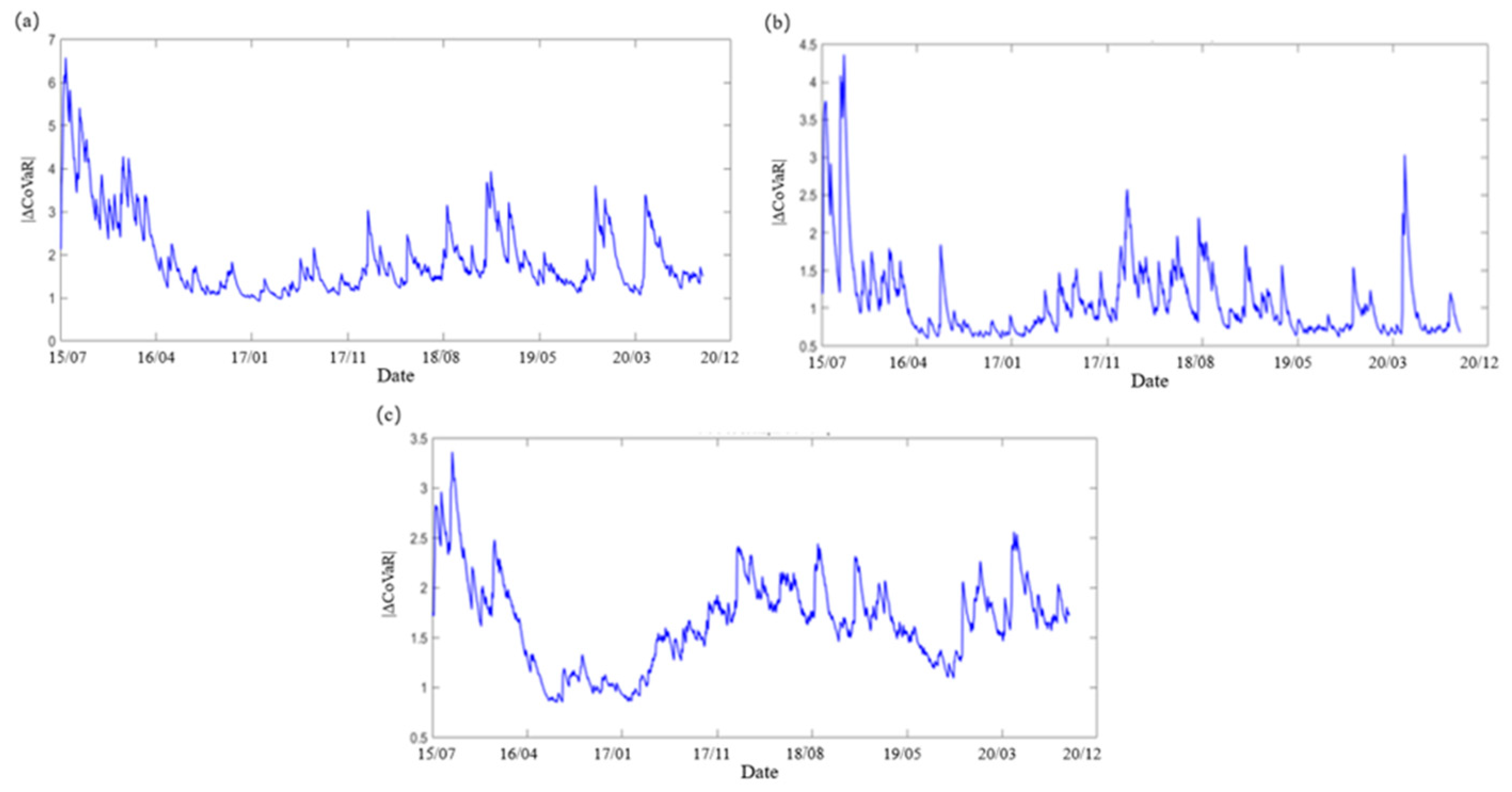
Figure 2.
Complex network model of A-share financial mark.
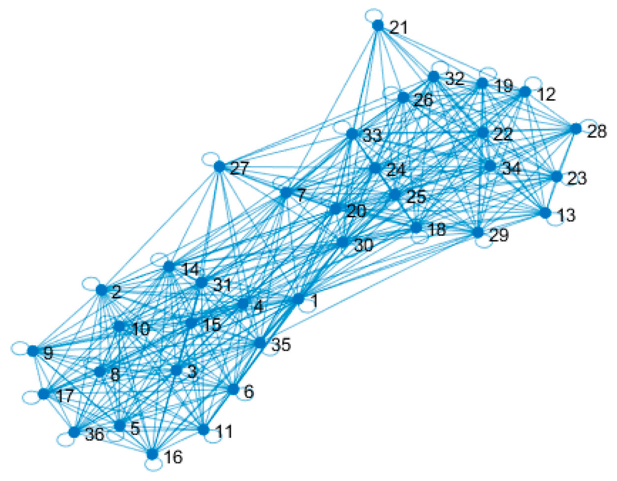
Figure 3.
Spectrum clustering results of A-share listed financial institutions.
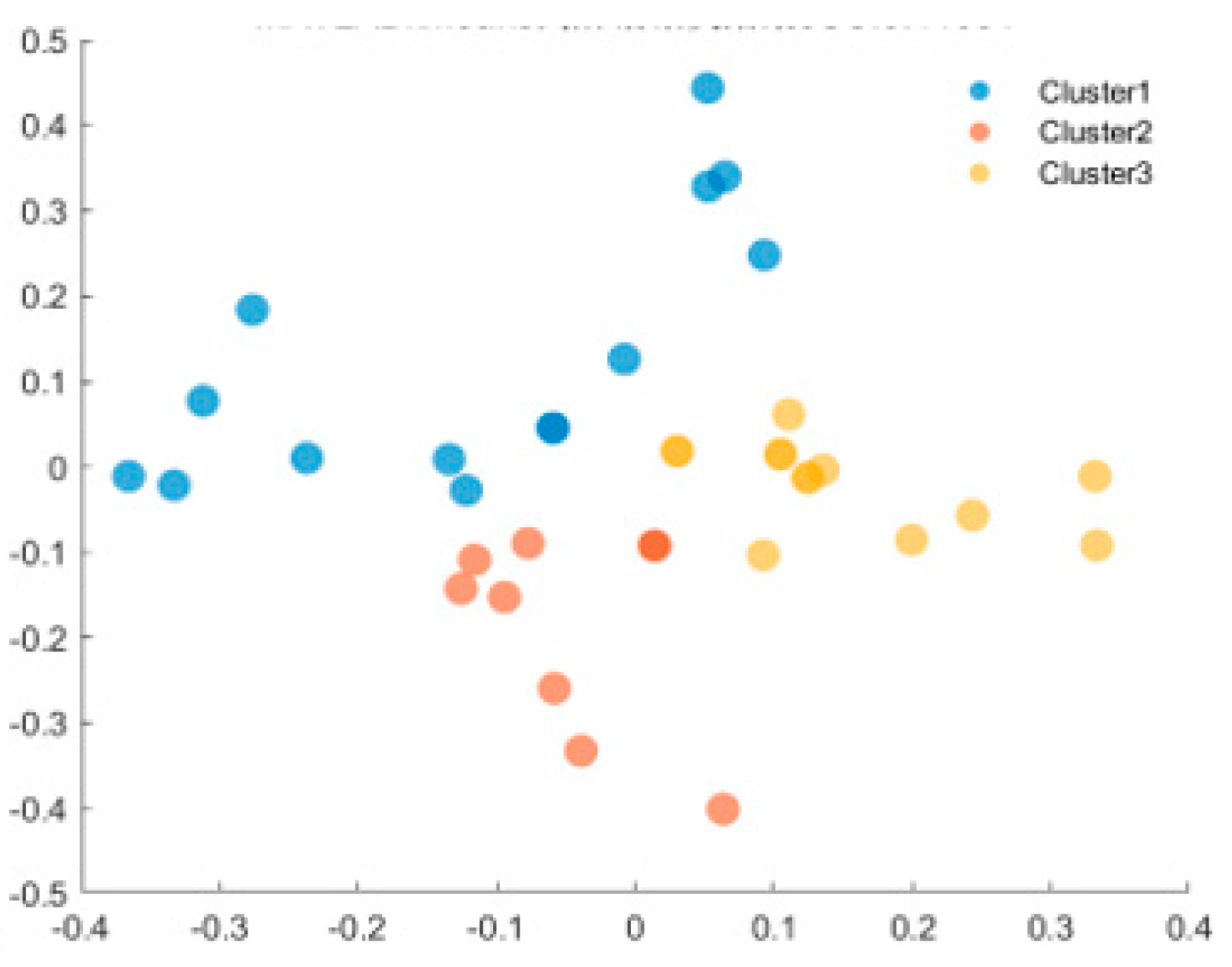
Figure 4.
Daily weighted average value of the three clusters from 2019 to 2020.
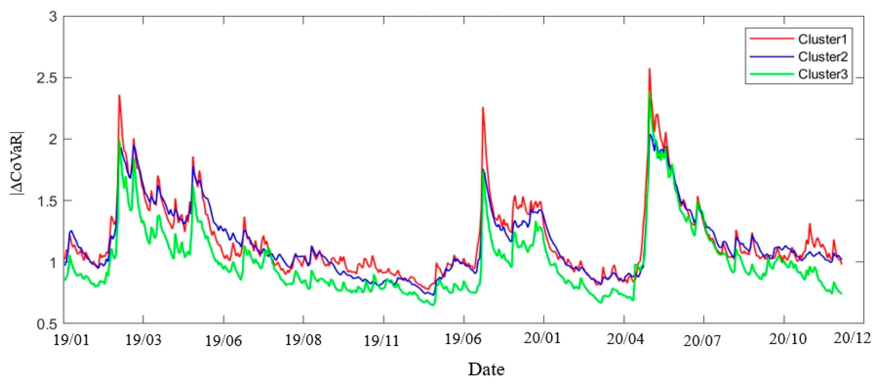
Figure 5.
Single-step prediction by RDPM and RBF neural network.
Figure 6.
Relative prediction accuracy of the three clusters.
Figure 7.
The trend of hit ratio.
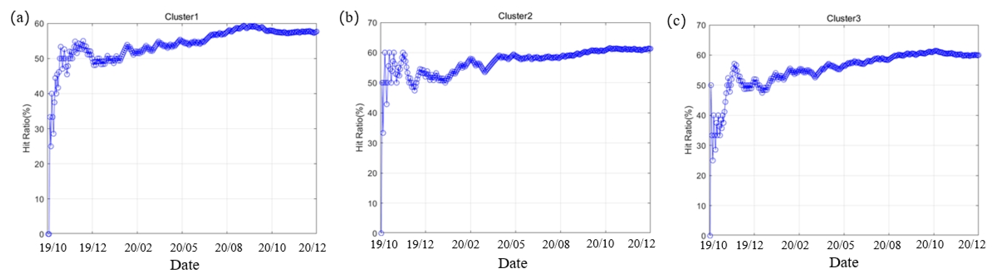
Figure 8.
Comparison of machine learning model predictions (RBF(a), SVM(b), LSTM(c) in turn).
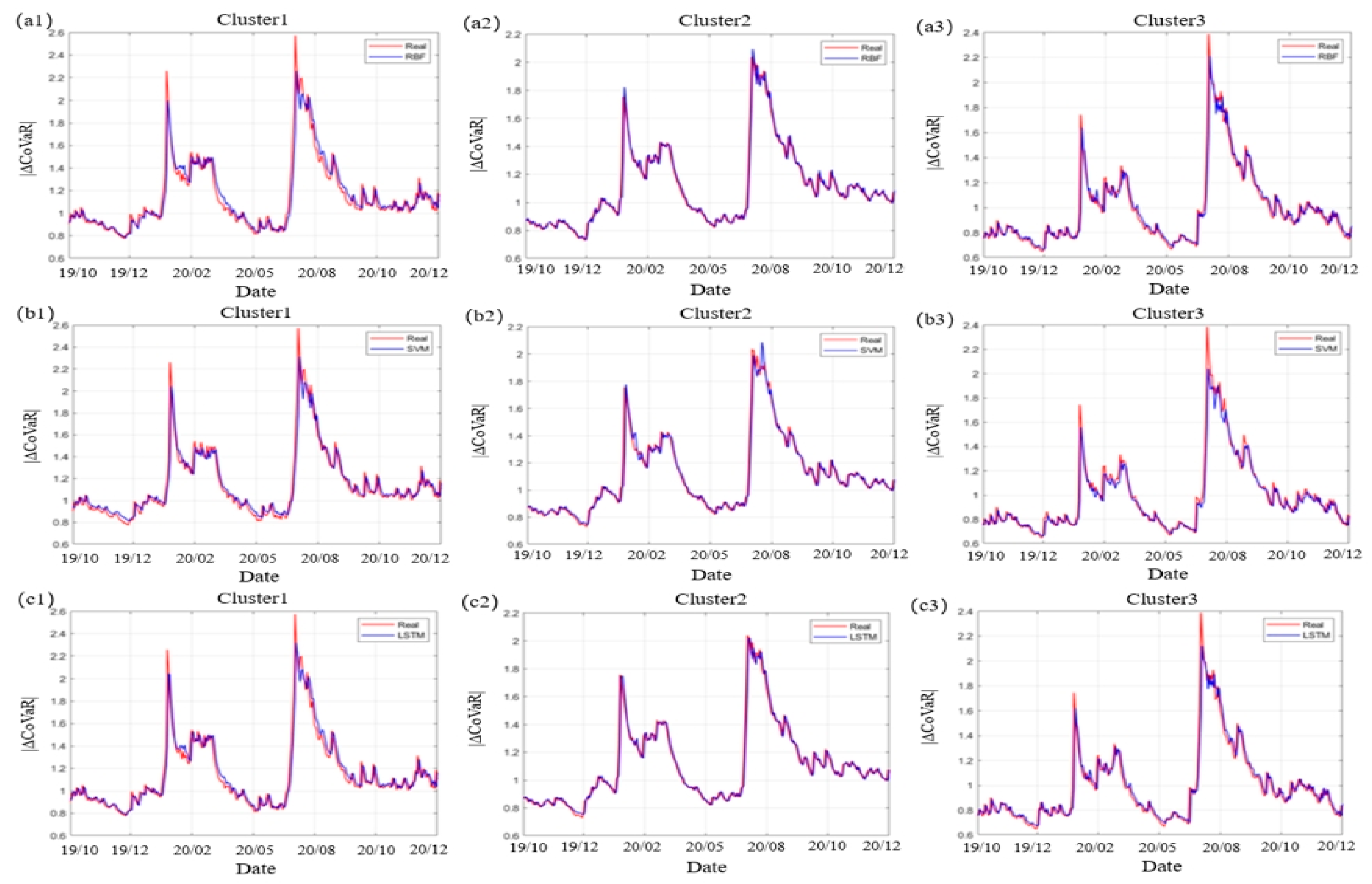
Figure 9.
Single-step prediction with weekly data.
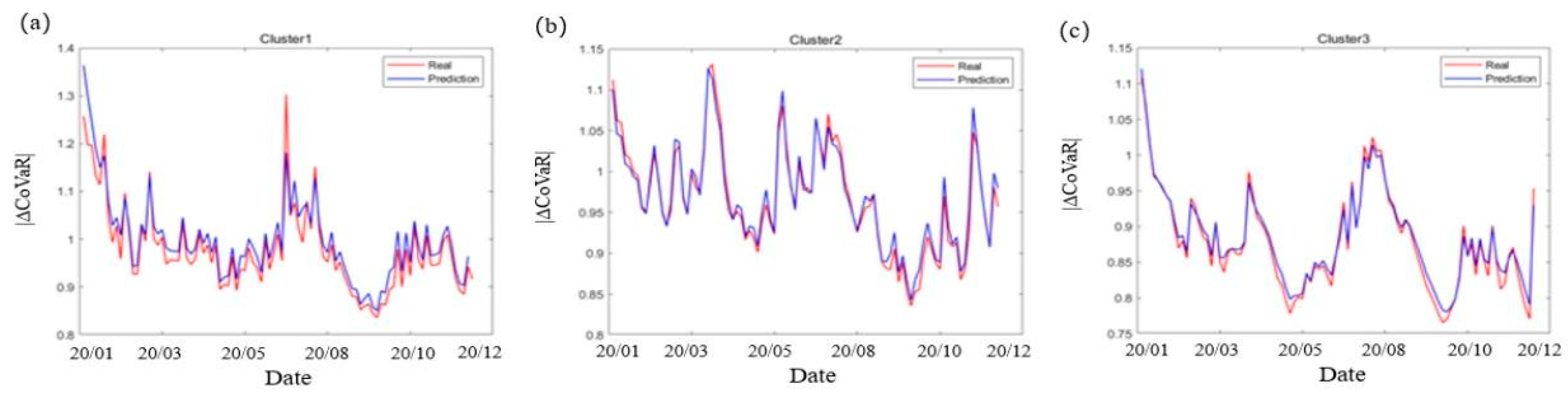
Figure 10.
Single-step prediction for 2021-2022.
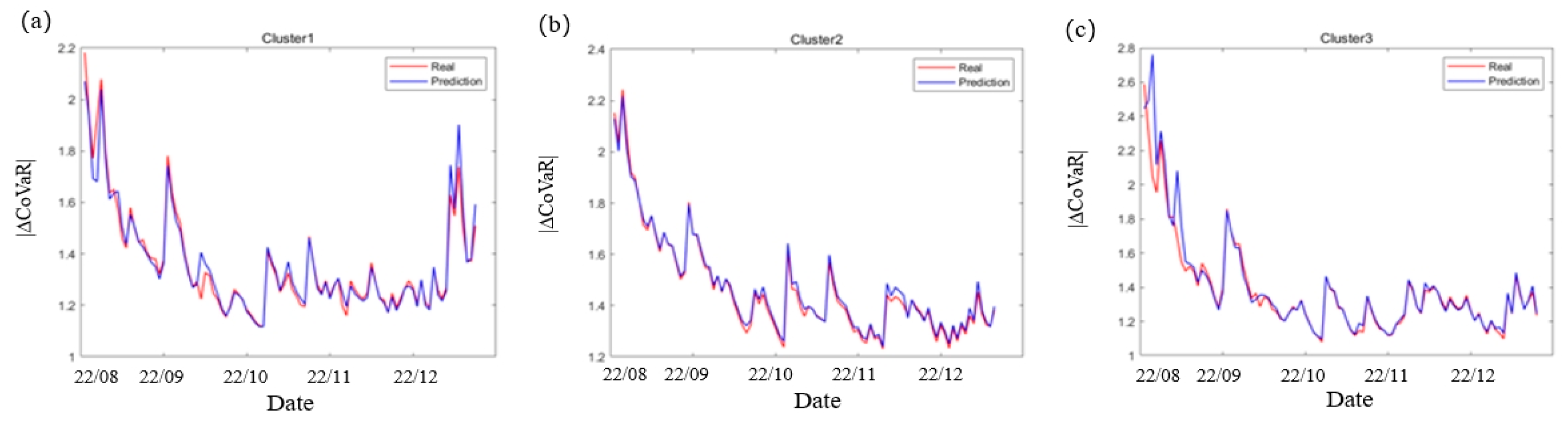
Figure 11.
Multi-step prediction days and corresponding error(MAE(a)、MSE(b)、RMSE(c)).
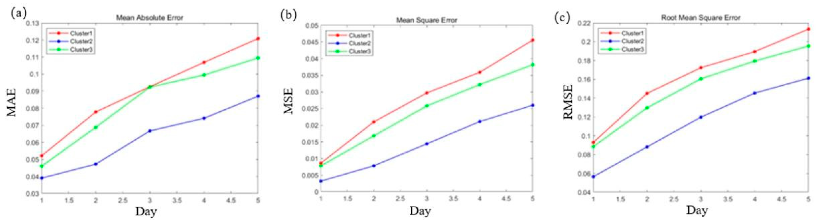
Figure 12.
Detection of systemic risk outliers.
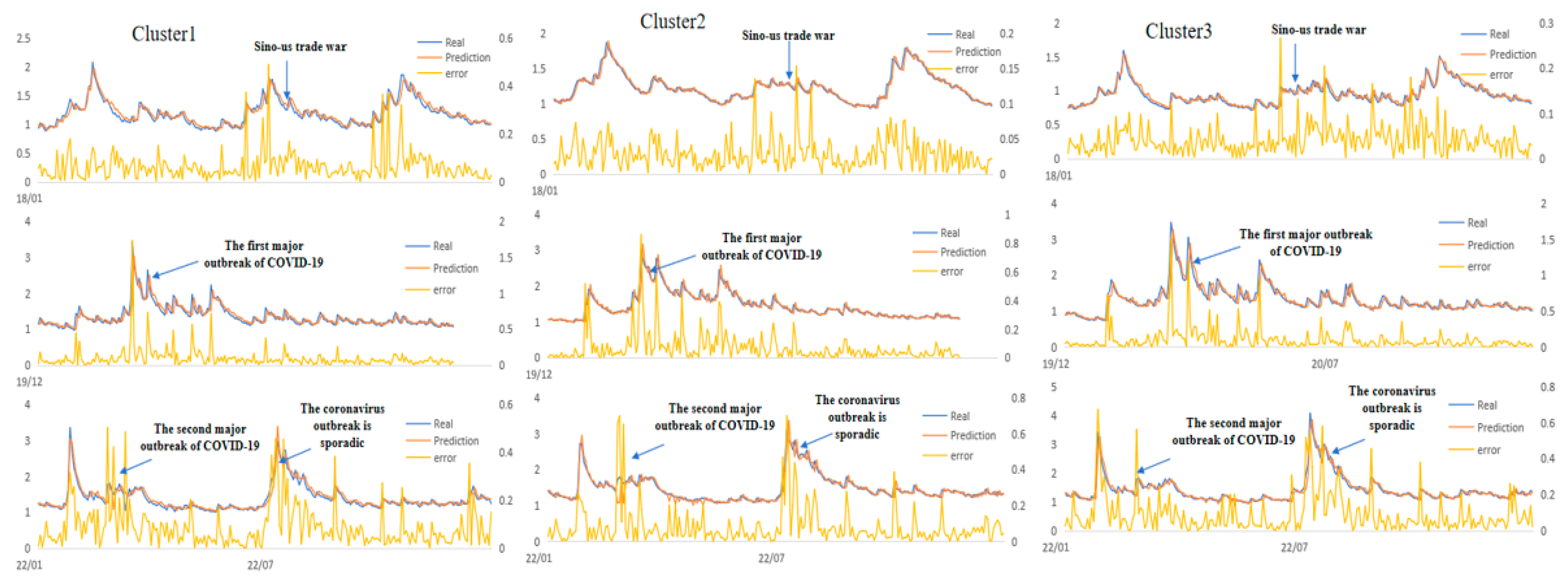
Table 1.
Average value of for financial institutions.
| Financial Institution | Financial Institution | ||
|---|---|---|---|
| SXS | 2.2872 | CMB | 1.1922 |
| HS | 2.1251 | CEB | 1.0941 |
| GJS | 1.9361 | ABC | 1.0910 |
| GS | 1.9247 | BCM | 1.0125 |
| ES | 1.9081 | CMBC | 1.0091 |
| PAIC | 1.8339 | WS | 0.9679 |
| NCLI | 1.8292 | CIB | 0.9196 |
| CMS | 1.7645 | BOC | 0.8871 |
| SCS | 1.6968 | ICBC | 0.6465 |
| CPIC | 1.6620 | SAJ | 0.6248 |
| OS | 1.6138 | CNCB | 0.3342 |
| CS | 1.5473 | SHS | 0.2984 |
| DS | 1.5413 | PS | 0.2651 |
| HB | 1.4445 | SPDB | 0.2037 |
| CLIC | 1.3602 | SITC | 0.0971 |
| NJCB | 1.3593 | BOB | 0.0703 |
| CCB | 1.2431 | FS | 0.0692 |
| NBCB | 1.2100 | IS | 0.0189 |
Table 2.
Average value of for three industries.
| Industry | Bank | Security | Insurance |
|---|---|---|---|
| 0.9145 | 1.3309 | 1.6713 |
Table 3.
Indicators related to complex networks.
| Node number |
Average degree |
Average degree centrality |
Average Path length |
Network diameter |
Network density |
|---|---|---|---|---|---|
| 36 | 20.72 | 0.592 | 1.443 | 3 | 0.296 |
Table 4.
Nodes and degree centrality of complex network.
| Financial Institution | Degree Centrality | Financial Institution | Degree Centrality |
|---|---|---|---|
| GJS | 0.8857 | CCB | 0.5428 |
| OS | 0.8571 | BOB | 0.5428 |
| DS | 0.8285 | NBCB | 0.5428 |
| SHS | 0.7428 | NJCB | 0.5428 |
| GS | 0.7428 | BCM | 0.5142 |
| WS | 0.7142 | CNCB | 0.5142 |
| NCLI | 0.7142 | PAIC | 0.5142 |
| SCS | 0.7142 | CIB | 0.5142 |
| FS | 0.6857 | CLIC | 0.4857 |
| SXS | 0.6571 | ICBC | 0.4857 |
| IS | 0.6571 | BOC | 0.4857 |
| CEB | 0.6571 | HB | 0.4857 |
| ABC | 0.6571 | CS | 0.4857 |
| HS | 0.6 | CMB | 0.4857 |
| CMS | 0.5714 | CMBC | 0.4857 |
| ES | 0.5714 | SPOB | 0.4857 |
| PS | 0.5714 | SAJ | 0.4571 |
| CPIC | 0.5714 | SITC | 0.3428 |
Table 5.
Spectrum clustering results of 36 financial institutions.
| Industry | Cluster1 | Cluster2 | Cluster3 |
|---|---|---|---|
| Bank | CIB,CEB,NJCB, | ABC,BOC,CMB, | BOB,NBCB, |
| CNCB,CMBC | ICBC,CCB,SPOB | BCM,HB | |
| Security | GJS,OS,SCS,GS, | DS,WS, | SHS,FS, |
| SXS,CMS,CS | IS,PS | HS,ES | |
| Insurance | PAIC,SAJ | NCLI,CPIC, SITC | CLIC |
Table 6.
Descriptive statistical characteristics of weighted average value.
| MAX | MIN | MEAN | |
|---|---|---|---|
| Cluster1 | 6.901 | 0.697 | 1.226 |
| Cluster2 | 2.992 | 0.708 | 1.216 |
| Cluster3 | 3.866 | 0.605 | 1.034 |
Table 7.
Prediction error by RDPM.
| MSE | MAE | RMSE | |
|---|---|---|---|
| Cluster1 | 0.0086 | 0.0511 | 0.0920 |
| Cluster2 | 0.0030 | 0.0295 | 0.0601 |
| Cluster3 | 0.0093 | 0.0584 | 0.1041 |
Table 8.
Comparison of errors with different machine learning methods.
| Model | MAE | MSE | ||
|---|---|---|---|---|
|
Cluster1 |
RDPM RBF SVM LSTM |
0.9123 0.8934 0.9066 0.9058 |
0.0511 0.0568 0.0529 0.0551 |
0.0086 0.0105 0.0092 0.0092 |
|
Cluster2 |
RDPM RBF SVM LSTM |
0.9613 0.9592 0.9592 0.9603 |
0.0295 0.0293 0.0393 0.0293 |
0.0030 0.0032 0.0031 0.0031 |
|
Cluster3 |
RDPM RBF SVM LSTM |
0.8990 0.8573 0.8816 0.9162 |
0.0584 0.0601 0.0685 0.0465 |
0.0093 0.0173 0.0195 0.0077 |
Table 9.
Prediction error of weekly data by RDPM.
| MSE | MAE | RMSE | |
|---|---|---|---|
| Cluster1 | 0.0056 | 0.0603 | 0.0745 |
| Cluster2 | 0.0035 | 0.0316 | 00592 |
| Cluster3 | 0.0081 | 0.0353 | 0.0899 |
Table 10.
Descriptive statistical characteristics of (2021-2022).
| MAX | MIN | MEAN | |
|---|---|---|---|
| Cluster1 | 3.878 | 1.019 | 1.379 |
| Cluster2 | 3.159 | 1.002 | 1.472 |
| Cluster3 | 4.084 | 0.961 | 1.387 |
Table 11.
Prediction error for 2021-2022.
| MSE | MAE | RMSE | |
|---|---|---|---|
| Cluster1 | 0.0087 | 0.0338 | 0.0933 |
| Cluster2 | 0.0078 | 0.0469 | 0.0882 |
| Cluster3 | 0.0115 | 0.0711 | 0.1072 |
Disclaimer/Publisher’s Note: The statements, opinions and data contained in all publications are solely those of the individual author(s) and contributor(s) and not of MDPI and/or the editor(s). MDPI and/or the editor(s) disclaim responsibility for any injury to people or property resulting from any ideas, methods, instructions or products referred to in the content. |
© 2025 by the authors. Licensee MDPI, Basel, Switzerland. This article is an open access article distributed under the terms and conditions of the Creative Commons Attribution (CC BY) license (http://creativecommons.org/licenses/by/4.0/).
Copyright: This open access article is published under a Creative Commons CC BY 4.0 license, which permit the free download, distribution, and reuse, provided that the author and preprint are cited in any reuse.


