
Submitted:
22 April 2025
Posted:
23 April 2025
You are already at the latest version
Abstract
This paper presents the optimal sizing of a hybrid renewable energy system (HRES) for 12 an isolated residential building using a modified Smell Agent Optimization (mSAO). The paper 13 introduces a time-dependent approach that adapts the selection of the original SAO control param-14 eters as the algorithm progresses through the optimization hyperspace. This modification addresses 15 issues of poor convergence and suboptimal search in the original algorithm. Both the modified and 16 standard algorithms were employed to design an HRES system comprising photovoltaic panels, 17 wind turbines, fuel cells, batteries, and hydrogen storage, all connected via a DC-bus microgrid. The 18 components were integrated with the microgrid using DC-DC power converters and supplied a 19 designated load through a DC-AC inverter. Multiple operational scenarios and multi-objective cri-20 teria, including techno-economic metrics such as Levelized Cost of Energy (LCOE) and Loss of 21 Power Supply Probability (LPSP), were evaluated. Comparative analysis demonstrated that mSAO 22 outperforms the standard SAO. Simulation results highlighted that the PV-wind turbine-battery 23 system achieved the best economic performance using SAO and mSAO. The mSAO reduced the 24 total annual cost (TAC) to approximately $614,288.8 and the levelized cost of energy (LCOE) to 25 (0.6868477489) $0.013/kWh, compared to the SAO which obtained a TAC, $615217 and the LCOE, 26 (0.7108991366) $0.077/kWh respectively.
Keywords:
Energy Management
; Hybrid Renewable Energy System (HRES)
; Meta-heuristic Algorithms
; Multisource
; Optimal Sizing
; Smell Agent optimization (SAO)
1. Introduction
Renewable energy sources have been utilized to decrease reliance on fossil fuels and reduce greenhouse gas emissions [1]. However, to address the intermittency issues of renewable sources, such as solar and wind, hybrid renewable energy systems (HRES) have been introduced as a solution. These systems not only meet electricity demand but also lower greenhouse gas emissions, providing an efficient, sustainable, and eco-friendly approach. This contributes significantly to the development of smart grid environments. Various configurations are integrated to develop a hybrid renewable energy system, either in grid-connected or stand-alone mode, using multiple energy sources to meet the energy demand. The system utilizes multiple storage devices to balance energy fluctuations, storing excess energy in the short term with batteries and supercapacitors, and in the long term with hydrogen tanks [2].
The optimal design of stand-alone hybrid renewable energy systems requires effective capacity planning and sizing to minimize investment costs and maximize the efficient use of hybrid energy resources. This design process must account for the coordination between energy sources, storage systems, and load demand patterns. To address sizing challenges in these systems, optimization techniques have been explored in the literature, involving mathematical modeling of components and the use of hourly weather data for the chosen location [3]. Additionally, these models focus on specific objective functions. In [4], the authors applied the PSO algorithm and an Artificial Neural Network to estimate PV panel parameters, with simulation results demonstrating a 3.5% improvement in convergence speed.
Recent research has focused on the performance of meta-heuristic algorithms for renewable energy system sizing. Several optimization techniques have been explored, including the Smell Agent Optimization (SAO) algorithm, a novel meta-heuristic inspired by the human sense of smell, which operates in three distinct modes: sniffing, trailing, and random mode, as described in [5]. The authors proposed an enhanced SAO algorithm for sizing hybrid renewable energy systems using photovoltaic panels, wind turbines, and batteries. This approach optimized the system for the lowest annual cost and minimized the Loss of Power Supply Probability (LPSP), with improvements of 79% and 53.4%, respectively. Similarly, in [6], the authors analyzed and compared the energy performance of different configurations, testing fuel cells (FC), electrolyzers, and hydrogen tanks as backup storage systems alongside photovoltaic panels (PV) and wind turbines (WT). The optimization results indicated that the PV/WT/FC configuration was the most cost-effective, achieving the lowest Total Annual Cost (TAC). In [7], Shuang Wang et al. demonstrated that while the original SAO algorithm is reliable for solving numerical problems, they improved the algorithm by incorporating the jellyfish swarm’s active-passive mechanism and a novel random operator. This modified SAO (mSAO) improved solution quality by 10–20% over the basic SAO when applied to constraint benchmarks and engineering problems.
Several algorithms have been developed to solve complex problems, including discrete, constraint, dynamic, and non-differentiable issues, as highlighted by Mariye Jahannoosh et al. in [8]. The hybrid Grey Wolf Optimizer-Sine Cosine Algorithm (HGWOSCA) was compared with the SCA, GWO, and Particle Swarm Optimization (PSO) methods for designing various combinations of hybrid systems under varying reliability constraints. The results demonstrated that the PV/WT/FC combination was the most cost-effective and reliable, particularly in terms of the lowest Levelized Supply Cost of Energy (LSCS) and the highest Load Instantaneous Power (LIPmax) for meeting the demand of remote communities. Additionally, the same system was analyzed using the Jaya algorithm and compared with the Genetic Algorithm, Backtracking Search Algorithm, and PSO. The simulation results, as shown in [9], revealed that the PV-FC system was the most cost-effective method, outperforming the PV-WT-FC and WT-FC combinations when the maximum Loss of Power Supply Probability (LPSP) was set at 0% and 2%. Recent studies have also led to the development of novel hybrid algorithms, such as the Smell Agent Optimizer (SAO) combined with Symbiosis Organism Search (SOS), as described in [10], for optimal control of microgrid operations. The findings suggest that the SASOS algorithm is a promising solution for engineering optimization and improving the control systems of autonomous microgrids.
Muhammad et al. in [11] presented an off-grid hybrid renewable energy system for electrifying a remote area in Abuja, Nigeria. The optimization problem was addressed using the Optimal Foraging Algorithm (OFA), and the results were compared with those from the Genetic Algorithm (GA) and Particle Swarm Optimization (PSO). Additionally, in [12], the authors proposed a Power Management and Control (PMC) system for energy optimization in sustainable environments. This system combines GA and PSO to balance energy consumption and the Occupant Comfort Index (OCI). The PMC system outperformed existing models by achieving an ideal OCI of 1 while using less energy. It was validated through simulations using actuators to control the indoor environment, demonstrating its effectiveness in reducing energy consumption while maintaining or enhancing comfort. Yan Cao et al. in [13] introduced a new model of the Elephant Herding Optimization (BEHO) Algorithm to solve multi-objective optimization problems. The algorithm was validated through various benchmark functions and algorithms for a proposed hybrid system based on PV, wind, fuel cell, and battery technologies. Recently, global attention has focused on optimizing energy management strategies for hybrid renewable energy systems, requiring careful coordination of design state, geophysical conditions, load demand, and parametric constraints. Effective implementation ensures project longevity, and cost-efficiency, and promotes sustainable development. Studies [14,15,16,17,18,19] highlight the technical and economic evaluation of excess electricity management beyond optimal storage capacity for off-grid renewable systems.
The main contributions of this paper are highlighted as follows:
- i.
- The paper presents a modified version of the Smell Agent Optimization (SAO) algorithm, which uses a time-dependent approach to adapt the control parameters dynamically as the algorithm progresses. This modification improves convergence and search efficiency, addressing the limitations of the original SAO algorithm.
- ii.
- The paper applies both the modified and standard SAO algorithms to design a hybrid renewable energy system (HRES) for an isolated residential building, in Annaba Algeria. The system includes photovoltaic panels, wind turbines, fuel cells, batteries, and hydrogen storage, all integrated with a DC-bus microgrid.
- iii.
- Through simulations, the paper proved that, modified SAO (mSAO) outperformed the standard SAO in terms of economic performance, reducing the total annual cost (TAC) to approximately $614288.8 and the levelized cost of energy (LCOE) to $0.013/kWh, compared to the TAC, $615217 and the LCOE, $0.077/kWh achieved by the SAO, ensuring optimal power delivery and maximizing project profitability over the HRES lifetime.
The paper is organized as follows: First, the introduction is provided. Section 2 presents the mathematical descriptions of all components in the DC multisource system, along with the problem formulation, including the objective function and constraints. In Section 3, the optimization approaches are defined. Section 4 discusses the energy management system of the proposed framework, utilizing the SAO and mSAO optimization techniques. The simulation results and corresponding discussion are covered in Section 5. Finally, conclusions and future research directions are suggested in Section 6.
2. Configuration of the System Under Study
This study focuses on a residential application using a multi-source hybrid renewable energy system (MHRES) connected to a DC bus to supply an AC dynamic load based on daily load data, with a maximum power of 4.9 kW. The primary goal is to enhance the system’s resilience by ensuring continuous power delivery to meet demand [20,21]. The system includes photovoltaic (PV) panels and a wind turbine to supply the load, along with a storage system consisting of batteries and a hydrogen storage tank. The parameters related to the components are presented in Table A1, Appendix A. The proposed system is shown in Figure 1, while the data used for the modeling are shown in Figure 2.
As illustrated in Figure 2, The Figure 2(a) displays the 24-hour load profile of a residential building in Anaba, Algeria. This profile exhibits a fluctuating energy demand throughout the day, with periods of low consumption during the early morning hours (approximately 0-6 hours), followed by increasing demand in the morning, a significant peak around midday (approximately 12-14 hours reaching nearly 5 kW), and subsequent fluctuations with a generally decreasing trend towards the late evening.
Figure 2(b) presents the corresponding 24-hour profiles for solar radiation and wind speed in Annaba. The blue line, plotted against the left y-axis, shows the solar radiation (in W/m²). It indicates a typical daytime solar irradiance pattern, starting at zero during the night, gradually increasing after sunrise, reaching a peak intensity around midday, and then decreasing back to zero as the sun sets. The orange line, plotted against the right y-axis, depicts the wind speed (in m/s). This profile shows more variability throughout the day, with periods of relatively low wind speeds and instances of higher wind speeds occurring at different times within the 24 hours. These solar and wind profiles capture the
2.1. System Modeling
The model examined in this study is a hybrid system comprising a solar system, fuel cell, and wind turbine integrated with electrolyzer and cell stacks (wind/solar/fuel cell) for prolonged energy utilization with stored energy for specific durations. During operation, excess electrical energy generated by the photovoltaic (PV) panels and wind turbine is utilized to charge the battery when SOC battery is less than SOC min or to produce hydrogen via electrolysis. Subsequently, the produced hydrogen is stored in hydrogen reservoir tanks, which are then utilized to generate electricity by providing fuel cell stacks with hydrogen.
The mathematical models of all components included in the proposed hybrid system are briefly presented as flow:
- A.
- PV model
The electrical power generated from series-connected several PV cells is expressed as follows [21,22]:
where I (t) is the solar radiation, A denotes the PV area and ηPV is the efficiency of PV system and converter system with number of PV panels, the total produced power is:
- B. Wind turbine model
The power of the wind turbine at a specific wind speed v can be formulated as follows [21,22]:
where v is the wind speed, Pr is the rated power of the WT, and vcut-in, vcut-out, and vr are cut-in, cut-out, and rated speed of the WT, respectively. If the number of WTs is ,the overall produced power is:
- C. Energy Storage
To maintain a continuous balance between energy sources and load, the Energy Storage System (ESS) can provide a regulating reserve. In our work, battery banks with fully integrated electrolyzer, fuel cells, and hydrogen tank systems are complemented to meet the required load.
The power balance is calculated as the difference between the total power generated ( ) by both the PV and wind and the power load. This value indicates whether there is a surplus or deficit of energy relative to the demand.
C.1 Battery storage
Potentially leading to a positive (excess energy) and the could be negative, indicating a deficit of energy. The charging and discharging schedule of
the battery is expressed in eqs. (6 to 9) in [23].
- Charging mode, when there is excess energy i.e :
The energy stored in the batteries can be calculated as the expression (7):
- Discharging mode, when there is deficit energy i.e:
The energy stored in the battery can calculated as the equation (9):
The SoCb can be expressed in a discrete form in [20]:
where, SoCb is the state charge of the battery and Pb is the battery power in (W), Eb,u is the nominal energy capacity in (Wh) of each elemental battery unit and nb is the number of batteries. It is assumed positive in the discharge process and negative when it is charging.
C.2 Water Electrolyzer
When there is an excess of energy, hydrogen is produced. The power output delivered from the electrolyzer to the tank of the hydrogen is illustrated as follows [23]
where Pel is the electrolyzer output power (kw), Pren_el is the electrolyzer input power (kw), and ηel is the efficiency of the electrolyzer assigned a constant value.
The amount of renewable energy available is determined by the amount of excess energy and the amount of energy used to charge the batteries.
Taking into account the rated power of the electrolyzer Peln and the charge level ofthe hydrogen tank, the following equation determines the actual amount of hydrogenproduced in [23]:
C.3 Modeling H2 Tank
The electrical energy stored inside the tank can be expressed as follows:
The amount of hydrogen stored in kilograms can be obtained from Equation (15) in [23]:
where, is the hydrogen gas higher heating value, which is usually taken as 39.7 [23].
C.4 Fuel Cell model
Proton Exchange Membrane Fuel Cells (PEMFC), one of the most widely utilized fuel cell technologies. This type of fuel cell generates only electricity, water, and heat.
The energy output of fuel cells is directly related to the hydrogen consumed from the hydrogen tank and the efficiency of the fuel cell as expressed in equation (16) as in [23].
- D. Inverter model
The inverter model is expressed in terms of the output power delivered to the load as follows in [23]:
2.2. Problem Formulation
The meta-heuristic algorithms, standard SAO, and modified mSAO algorithms are applied to generate the optimal design and sizing of the proposed systems. The objective function describing the entire system and all the relevant constraints are presented in this section.
2.2.1. Objective Function
The optimal design of the hybrid systems is proposed to minimize the level cost of energy (LCOE), the Loss of Power Supply Probability (LPSP), and excesses energy (EE). The corresponding mathematical expression is given by the Equation below in [24]:
The objective functions can be expressed in Eqs (21 to 29)
where, Total Annual Cost (TAC), present the total energy produced and N stands for the overall number of hours considered, ACC for annualized capital cost, and AMC for the annual maintenance and REPC for replacement cost. The AMC is calculated using Eq. (23) in [5]:
The ACC, on the other hand, is calculated using Eq. (24) in [5] as follows:
where represents the number of PV, wind turbine, batteries, hydrogen tank and converter, respectively, while denote the unit costs of the PV, wind turbine, fuel cell, electrolyzer, batteries and converter, respectively. CRF is the Capital Recovery Factor is modeled in [5] as:
where I (5%) is the annual interest rate and n denotes the system’s lifetime (20 years).
The replacement cost (REPC) is calculated using Eq. (26-27) in [25]:
where, nr is the lifetime of the replaced component.
The loss of power supply probability (LPSP) is a criterion used for evaluating the reliability of the proposed energy system. The equation below is used to calculate the value of the LPSP in [23].
The following mathematical equation can be used to express the excesses of energy [23]:
2.2.2. Different Constraints
The tri-objective function must be optimized considering system components minimum and maximum number N Lower ≤ Ni ≤ N Upper as decision variable constraints related to the optimal design and sizing of the HRES that should be satisfied:
3. Optimization Approaches for Microgrid Energy Management
The majority of new metaheuristics algorithms was focused on the foraging behaviors of the agents through a constant parameterization [24]. The SAO is one such algorithm whose performance is significantly influenced by the choice of its control parameters, like the olfaction capacity and step size. In our study we proposed a dynamic method for selecting these parameters and eventually proposed a modified SAO, called the mSAO. Both the mSAO and the original SAO were used to obtain the optimal results for sizing the hybrid renewable energy system based on established reliability, technico-economical and stability criterion. To attain optimal solutions for microgrid energy management (EMS) issues characterized by diverse limitations and uncertainties, optimization approaches based on multiple management strategies were proposed in Figure B1, Appendix B.1 in [26].
3.1. Smell Agent Optimizer
Smell Agent Optimization (SAO) is a cutting-edge metaheuristic algorithm inspired by the intelligent behaviors of agents trailing the source of a smell molecule. This modern optimization technique mimics the natural process of smell detection and tracking, where agents navigate through a complex search space to identify the optimal solution [27]. The SAO combines swarm intelligence, machine learning, and dynamic optimization principles to efficiently explore and exploit the search space, ensuring a robust and adaptive search process. The parameters related to the SAO algorithm are given in Table A2, Appendix A. Detail theoretical information on the SAO algorithm can be found in [24,27].
The SAO algorithm is defined by a set of equations in three main phases, which model the behavior of agents as they search for optimal solutions.
The SAO begins by initializing a population of smell molecules, represented as candidate solutions:
where denotes the matrix of current solutions, and d is the number of control variables in the problem domain.
Each molecule’s position is based on upper and lower bounds:
where is a random number between 0 and 1, and ub and lb ,are the upper and lower bounds of the variable.
- Sniffing Mode: Initial exploration of the search space.
Through Brownian motion with each molecule having a velocity given by:
The molecules update their positions using:
where is updated by:
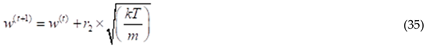
where: k is Boltzmann’s constant (smell constant), T is the temperature of molecules, m is the mass of molecules, r2 is a random value.
- 2.
- Trailing Mode: Agents follow the best solution found.
Agents adjust their positions to move toward promising solutions. The new position is computed using:
where: rD, rJ,are random numbers between [0,1], olf is the olfaction capacity, is the best solution found, is the worst solution.
- 3.
- Random Mode: Random exploration to avoid local optimal.
If the algorithm fails to improve fitness using sniffing or trailing modes, the random mode is activated:
where: step is an arbitrary constant step size, rK is a random number between (0, 1).
3.2. Modified Smell Agent Optimizer (mSAO)
The unique features of SAO, such as dynamic sniffing, trailing, random phases, and agent communication, enable the algorithm to balance exploration and exploitation effectively, leading to improved convergence and solution quality. Despite these positive features of the algorithm, the performance of each phase of the algorithm is highly dependent on the proper choice of its control parameters. For example, in the sniffing phase of the algorithm, the evaporation of smell molecules is penalized by the temperature (T), mass (M), and Boltzmann’s constant (K). In the trailing phase, the ability of the agent to trail the smell molecule is penalized by a constant olfaction capacity of the agent (olf), whereas, the random, phase is penalized by a constant step size (S). Poor choices of these parameters may result in inadequate exploration and exploitation of the search space, leading to insufficient diversity in solutions and reduced chances of finding global optima. This could also result in scalability problems, as the algorithm may not scale well with increasing problem dimensions or agent populations, leading to decreased performance and efficiency. To address these challenges, this paper introduces a mathematical procedure to adapt the selection of the control parameters as the algorithm progresses through the hyperspace. For example, the olfaction capacity and the step movement of the agent are mathematically determined using (31) and (32) respectively.
where, and are the lowest and highest possible values of olfaction capacity, and are the lowest and highest possible step an agent can take during random search, and are the maximum and current iterations respectively.
The SAO modification in (31) and (32) is implemented to linearly decreases with time. This means that, for the initial stages of the search process, large values are selected to enhance the global exploration, and searching new area is recommended while, for last stages, the parameter values are reduced for local exploration, fine-tuning the current search area effectively. The Flowchart for the implementation of the modified SAO is shown in Figure 3.
4. Multisource Model Energy Management Strategy
In our study, the proposed energy management used for the integrated multisource-based PV & WT generators and using batteries, green hydrogen for energy storage, was investigated. The primary objective is to ensure power balance and to minimize the operating costs of the system. Additionally, extending the life cycle is essential for system components, especially the fuel cell stack by reducing the FC power dynamics and conserving hydrogen use. However, the battery is fully charged to manage excess energy when the hydrogen storage tank is filled, and load demand is minimal. This approach ensures a consistent and reliable energy supply to meet demand. The proposed EMS optimization mechanisms are illustrated in Figure 4, following the definition of the system’s constraints and objective function.
5. Results and Discussion
This section presents the simulation results study of the proposed systems carried out on hourly weather and load demand data.
5.1. Optimization Technique Analysis
The results in Table 1 outline the sizing of renewable energy components obtained using the modified Smell Agent Optimization (mSAO) algorithm compared to the original Smell Agent Optimizer (SAO). The performance of the developed techniques is evaluated under three test scenarios. In the first scenario, all the systems components including the two storage types (Battery and Hydrogen Tank) are interconnected in the EMS. In the second scenario, the hydrogen is disconnected leaving only the battery system as the energy storage device. While, in the third scenario, the Battery system is disconnected, leaving only the Hydrogen Tank as the storage system. The best, average, and standard deviation have been calculated based on the results of the 50 executions. The modeling and simulation of the optimization problem have been accomplished using MATLAB R2023b program. All simulations were carried out on a HP computer system, with Windows 11 OS, 16GB of RAM, and Intel CORE i7, 10th Gen.
The results for the optimal sizing with EMS are summarized in Table 1.
It can be seen from Table 1 that; the analysis reveals that, the mSAO algorithm consistently outperforms the SAO algorithm across all configurations, as evidenced by the reduced number of components required and the associated decrease in total annual cost. The installed PV power is reduced with the mSAO in all configurations; this is mainly caused by the optimal distribution of power and the prediction capacity of the mSAO algorithm. However, wind turbines serve the same dimension in all configurations; the energy capacity of batteries is also reached with mSAO in the scenario 1 and fixed in scenario 2.
The depicted Figure 5 illustrates the convergence of the algorithms throughout 100 iterations, wherein the most optimal outcome is observed in the second configuration utilizing battery, contrasting with the other two configurations. Moreover, the efficiency of the mSAO algorithm in attaining optimal solutions by iteration number 29 correlates with a total annual cost of 614288.8 ($), as demonstrated by its consistently superior performance over a total of 50 runs as as shown in Figure 6, and Figure 7.
The results of different scenarios show the response of the proposed method to variation of input parameters indicating the effectiveness of the proposed optimization algorithm. From the results shown in Table 2, it can be observed that the mSAO reached the optimal objective function value in all cases much better than the standard SAO. The insignificant difference between the Best and Average values proved the convergence of the 50 implemented runs, demonstrating the stability and accuracy of the mSAO technique.
The analysis of the result shows the superior performance of the mSAO algorithm over the SAO algorithm across the key performance indicators. For the PV/WT/Battery/Hydrogen configuration, the average LCOE achieved by mSAO is approximately slightly higher than that achieved by SAO. The average LPSP with mSAO is significantly lower at 0.0144, compared to 0.3801 for SAO, representing a substantial reduction of roughly 96.2%. The average excess energy is slightly higher for mSAO at 17.164 GWh compared to 16.418 kWh for SAO, an increase of about 4.6%. Similarly, for the PV/WT/Battery configuration, the average LCOE for mSAO is about 3.9% higher than that of SAO. The average LPSP for mSAO is 0.0122, significantly lower than the 0.3149 for SAO, a reduction of approximately 96.1%. The average excess energy is marginally higher for mSAO at 17.304 kWh compared to 17.079 kWh for SAO, an increase of about 1.3%. Finally, for the PV/WT/Hydrogen configuration, the average LCOE for mSAO is also little higher than that obtained by SAO. The average LPSP is reduced from 0.3126 with SAO to 0.0105 with mSAO, a reduction of approximately 96.6%. The average excess energy is slightly higher for mSAO at 17.322 kWh compared to 17.069 kWh for SAO, an increase of about 1.5%. These comparative values across all configurations consistently highlight the significant improvements offered by the mSAO algorithm, more importantly, the LPSP.
Figure 8, illustrates the performance comparison of the two optimization algorithms, SAO and mSAO, across 50 runs for the three renewable energy system configurations: PV/WT/Hydrogen/Battery, PV/WT/Hydrogen, and PV/WT/Battery.
The mSAO exhibits improved stability and reduced fluctuations in total annual cost across all system configurations, with particular advantages in the complex PV/WT/Hydrogen/Battery setup. This improvement can be attributed to mSAO design, which incrementally narrows the range of search parameters in later iterations. By focusing more precisely on promising regions in the solution space, mSAO minimizes the occurrence of cost spikes, especially under more intricate conditions involving multiple energy storage options like hydrogen. In simpler configurations (PV/WT/Battery), while both algorithms show comparable performance, mSAO still consistently achieves marginally lower costs, suggesting a distinct robustness that favors complex system optimization where cost minimization and reliability are paramount.
Figure 9 compares the performance of the three renewable energy system configurations using three key metrics: Loss of Power Supply Probability (LPSP), Levelized Cost of Energy (LCOE), and Excess Energy. In terms of reliability, the PV/WT/Hydrogen system shows the lowest LPSP, indicating it is the most dependable configuration with the least chance of power supply failure. The PV/WT/Battery/Hydrogen system has a higher LPSP, but it achieves the lowest LCOE, making it the most cost-effective option over its lifetime. Meanwhile, both the PV/WT/Battery and PV/WT/Hydrogen systems show higher LCOE, which suggests they are less cost-efficient. When assessing energy efficiency, the PV/WT/Battery/Hydrogen system also excels by producing the least excess energy, indicating better energy utilization compared to the other two configurations. The PV/WT/Battery configuration, although simpler, produces the most excess energy, which suggests it is less efficient and incurs higher energy wastage. Overall, the PV/WT/Battery/Hydrogen system offers the best balance between cost-effectiveness and energy utilization, though the PV/WT/Hydrogen system stands out for its superior reliability.
Figure 10 which shows the results across the three scenarios—PV/WT/Hydrogen/Battery, PV/WT/Battery, and PV/WT/Hydrogen—highlight the cost distribution among key components: wind turbines (wtCost), photovoltaic panels (pvCost), batteries (batCost), and hydrogen tanks (tankCost). The optimization results show that the PV/WT/Hydrogen/Battery system generally incurs the highest total annual cost due to the inclusion of both battery and hydrogen storage, with substantial contributions from batCost and tankCost. However, this system offers the best balance for reliability due to its diversified energy storage options, making it a strong contender for projects prioritizing energy security despite higher costs. The PV/WT/Battery system has lower overall costs, particularly due to reduced tankCost, but it may be less reliable in scenarios requiring largescale energy storage, as it relies solely on batteries.
From an investment perspective, the PV/WT/Hydrogen system stands out as the best option, striking a favorable balance between total cost and system performance. While it eliminates the cost of batteries (batCost), it leverages the cost efficiency of hydrogen storage (tankCost) and maintains moderate wtCost and pvCost. This system provides a middle ground in terms of both cost and energy reliability, making it an optimal choice for investors looking to minimize capital expenditures while maintaining a reliable and efficient energy supply. Therefore, for projects focused on minimizing costs without compromising too much on energy reliability, the PV/WT/Hydrogen configuration is the most attractive scenario for investment.
6. Conclusion
This paper has successfully demonstrated the efficacy of modified Smell Agent Optimization (mSAO) algorithm in optimizing the design and operation of a hybrid renewable energy system (HRES) for an isolated residential building. By introducing a time-dependent adaptation of control parameters, the mSAO significantly improved upon the limitations of the standard SAO algorithm, leading to enhanced convergence and search capabilities. Through rigorous simulations and comparative analysis, the mSAO consistently outperformed the standard SAO in terms of both economic and reliability metrics. The proposed HRES, optimized using mSAO, achieved a lower total annual cost (TAC) and levelized cost of energy (LCOE) compared to the standard SAO, indicating superior economic performance. Furthermore, the system configuration comprising photovoltaic (PV) panels, a wind turbine, and a battery storage system was identified as the most cost-effective solution, capable of delivering optimal energy performance across various operational scenarios. The findings of this research highlight the potential of advanced optimization techniques like mSAO in enhancing the economic viability and operational efficiency of renewable energy systems. Future work could also focus on real-time control strategies and demand-side management techniques that enable more responsive and adaptive power distribution. This could include the application of machine learning algorithms to predict load demand and optimize energy storage management. Also, field validation of the proposed mSAO technique in real-world HRES installations would be invaluable in demonstrating its practical viability and scalability for larger, more complex systems.
Author Contributions
Manal.D.: Conceptualization methodology and writing—original draft, original draft preparation; editing; formal analysis. Ahmed .T.S.: Conceptualization, supervision and resources, reviewing and editing; formal analysis. Mourad.H: reviewing and supervision, Mebarek.B:reviewing. All authors have read and agreed to the published version of the manuscript.
Funding
This research received no external funding.
Institutional Review Board Statement
Not applicable.
Informed Consent Statement
Not applicable.
Data Availability Statement
The data presented in this study are available on request from the corresponding author.
Acknowledgments
The authors sincerely acknowledge the significant Editor and Reviewers for their useful contributions.
Conflicts of Interest
The authors declare no conflict of interest.
Appendix A
Nomenclature and Abbreviation List
|
Lower limit of solar panels number Upper limit of solar panels number Number of wind turbine Lower limit number of WT Upper limit number of WT Power balance Energy consumed to charge the batteries Energy supplied from the batteries to the load Fuel cells power output power Fuel cells rating power Amount of hydrogen generated Amount of hydrogen generated and stored Energy consumed by fuel cell to generate power Inverters rating power Energy available at (t) in the batteries Energy available in the batteries at (t-1) Nominal capacity of the batteries |
Battery self-discharge rate Efficiency of the solar panel Battery charging system efficiency Battery discharging efficiency Electrolyzer efficiency Fuel cells efficiency SOC state of charge of battery SOC min state of charge minimal of battery Upper limit of batteries capacity Energy available at (t) in the tank Energy available in the tank at (t-1) Hydrogen minimum permissible energy Nominal capacity hydrogen tank Lower limit number of hydrogen tank Upper limit number of hydrogen tank Lower limit number of Fuel cell Upper limit number of Fuel Cell Lower limit number of Electrolyzer Upper limit number of Electrolyzer Batteries minimum permissible energy Maximal capacity of the batteries Lower limit of batteries capacity |
Appendix A.1

Table A1.
HRES components specification and economic parameters. .
| Component systems | Parameters | Specifications |
| PV | Nominal Pv power Pr-Pv Pv cost CPv Surface area A Pv efficiency ηPV Pv lifetime |
120 W $216 1.07 m2 12% 20 years |
| Wind Turbine | Nominal Wt power Pr-Wt Vcut-in Vcut-out Vr CWind Maintenance cost CMntWind Wt lifetime |
1 kW 3 m/s 20 m/s 9 m/s $1804 $100 20 years |
| FC | Nominal FC power FC efficiency (ηFC) FC lifetime FC cost (CFC) Replacement cost (CMnt-FC) |
3 kW 50% 5 years $20000 $1400 |
| Battery | Energy capacity (Eb,u) Maximum discharge power (b,max) Maximum charge power (Pb,min) Maximum SoCb minimum SoCb Capital Cost (CCb) Equivalent full cycles (Ncycles,b) Maintenance cost (Com;b) |
1000 Wh 1000 W 1000 0.9 0.24 2000 $ 471 5% CCb $/year |
| Electrolyzer | Nominal electrolyzer power Electrolyzer efficiency (hEle) Electrolyzer lifetime Electrolyzer cost (CEle) Replacement cost (CMnt-Ele) |
3 kW 74% 5 years $20000 $1400 |
| H2Tank | Reservoir tanks cost (CHT) Nominal capacity of hydrogen tank |
$2000 0.3 kW |
| Converter | Power converter inverter efficiency (η conv/inv) Converter/inverter lifetime Converter/inverter cost |
3 kW 95% 10 years $1583 |
| Other parameters | Interest rate of project i lifespan of the project n |
5% 20 years |
Appendix A.2
Table A2.
SAO Metaheuristic algorithm related parameters.
| Parameter | Symbol | Value |
| Number of Smell Molecules | N | 50 |
| Number of the decision variable | D | 4 |
| Temperature | T | 3 |
| Mass | m | 2.4 |
| Boltzman’s constant | K | 1.38× |
| Maximum iteration | itr | 100 |
References
- De Vito, S., et al. Electric Transmission and Distribution Network Air Pollution. Sensors . (20240.24(2): 587.
- Sharaf MA, Armghan H, Ali N, Yousef A, Abdalla YS, Boudabbous AR, Mehdi H, Armghan A. Hybrid control of the DC microgrid using deep neural networks and global terminal sliding mode control with the exponential reaching law. Sensors. 2023 Nov 22;23(23):9342.
- Thirunavukkarasu GS, Seyedmahmoudian M, Jamei E, Horan B, Mekhilef S, Stojcevski A. Role of optimization techniques in microgrid energy management systems—A review. Energy Strategy Reviews. 2022 Sep 1;43:100899.
- Lo WL, Chung HS, Hsung RT, Fu H, Shen TW. PV Panel Model Parameter Estimation by Using Particle Swarm Optimization and Artificial Neural Network. Sensors. 2024 May 9;24(10):3006.
- Biliyok AS, Tijani SA. Improved Smell Agent Optimization Sizing Technique Algorithm for a Grid-Independent Hybrid Renewable Energy System. InRenewable Energy-Recent Advances 2022 Oct 12. IntechOpen.
- Drici M, Houabes M, Salawudeen AT, Bahri M. Optimum design of an off-grid PV/WT/FC/battery based microgrid for sustainable and cost-effective energy optimization. Studies in Engineering and Exact Sciences. 2024 Jul 3;5(2):e5438-.
- Shuang Wang , Abdelazim G. Hussien , Sumit Kumar, Ibrahim AlShourbaji and Fatma A. Hashim . A modified smell agent optimization for global optimization and industrial engineering design problems.Journal of Computational Design and Engineering, 2023, 10,2147–2176. [CrossRef]
- Mariye Jahannoosh , Saber Arabi Nowdeh , Amirreza Naderipour , Hesam Kamyab , Iraj Faraji Davoodkhani , Jiří Jaromír Klemeš .New Hybrid Meta-Heuristic Algorithm for Reliable and CostEffective Designing of Photovoltaic/Wind/Fuel Cell Energy System Considering Load Interruption Probability.journal of Cleaner Production . [CrossRef]
- Khan A, Javaid N. Optimal sizing of a stand-alone photovoltaic, wind turbine and fuel cell systems. Computers & Electrical Engineering. 2020 Jul 1;85:106682.
- Mohammed S, Sha’aban YA, Umoh IJ, Salawudeen AT, Ibn Shamsah SM. A hybrid smell agent symbiosis organism search algorithm for optimal control of microgrid operations. Plos one. 2023 Jun 7;18(6):e0286695.
- M. M. Muhammad, J. Usman, I. Mustapha, M. U. M. Bakura and A. T. Salawudeen .An independent framework for off-grid hybrid renewable energy design using optimal foraging algorithm (ofa). journal of engineering, technology & environment 2021, www.azojete.com.ng.
- Ali S, Hayat K, Hussain I, Khan A, Kim D. Optimization of Distributed Energy Resources Operation in Green Buildings Environment. Sensors. 2024 Jul 22;24(14):4742.
- Yan Cao , Hui Yao , Zhijie Wang , Kittisak Jermsittiparsert , Nasser Yousefi ,‘’Optimal Designing and Synthesis of a Hybrid PV/Fuel cell/Wind System using Meta-heuristics’’, Energy Reports 6 (2020) 1353–1362. [CrossRef]
- Xing X, Jia L. Energy management in microgrid and multi-microgrid. IET Renewable Power Generation. 2023 Oct 30.
- Chalal L, Saadane A, Rachid A. Unified Environment for Real Time Control of Hybrid Energy System Using Digital Twin and IoT Approach. Sensors. 2023 Jun 16;23(12):5646.
- Alhumade H, Rezk H, Louzazni M, Moujdin IA, Al-Shahrani S. Advanced energy management strategy of photovoltaic/PEMFC/lithium-ion batteries/supercapacitors hybrid renewable power system using white shark optimizer. Sensors. 2023 Jan 30;23(3):1534.
- Mbouteu Megaptche CA, Kim H, Musau PM, Waita S, Aduda B. Techno-Economic Comparative Analysis of Two Hybrid Renewable Energy Systems for Powering a Simulated House, including a Hydrogen Vehicle Load at Jeju Island. Energies. 2023 Nov 29;16(23):7836.
- Abdelwahab SA, El-Rifaie AM, Hegazy HY, Tolba MA, Mohamed WI, Mohamed M. Optimal Control and Optimization of Grid-Connected PV and Wind Turbine Hybrid Systems Using Electric Eel Foraging Optimization Algorithms. Sensors. 2024 Apr 7;24(7):2354.
- Ali S, Hayat K, Hussain I, Khan A, Kim D. Optimization of Distributed Energy Resources Operation in Green Buildings Environment. Sensors. 2024 Jul 22;24(14):4742.
- Rullo P, Braccia L, Luppi P, Zumoffen D, Feroldi D. Integration of sizing and energy management based on economic predictive control for standalone hybrid renewable energy systems. Renewable energy. 2019 Sep 1;140:436-51.
- Akbar Maleki . Modeling and optimum design of an off-grid PV/WT/FC/diesel hybrid system considering different fuel prices. Journal of Low-Carbon Technologies 2018, 13, 140–147.
- Maleki A, Pourfayaz F, Rosen MA. A novel framework for optimal design of hybrid renewable energy-based autonomous energy systems: A case study for Namin, Iran. Energy. 2016 Mar 1;98:168-80.
- Amoussou I, Tanyi E, Fatma L, Agajie TF, Boulkaibet I, Khezami N, Ali A, Khan B. The optimal design of a hybrid solar PV/Wind/Hydrogen/Lithium battery for the replacement of a heavy fuel oil thermal power plant. Sustainability. 2023 Jul 25;15(15):11510.
- Salawudeen AT, Mu’azu MB, Yusuf A, Adedokun AE. A Novel Smell Agent Optimization (SAO): An extensive CEC study and engineering application. Knowledge-Based Systems. 2021 Nov 28;232:107486.
- Douak M, Settou N. Techno-economical optimization of pv/wind/fuel cell hybrid system in Adrar region (Algeria). International Journal of Sustainable Development and Planning. 2021 Feb;16:175-80.
- Shafiullah M, Refat AM, Haque ME, Chowdhury DM, Hossain MS, Alharbi AG, Alam MS, Ali A, Hossain S. Review of recent developments in microgrid energy management strategies. Sustainability. 2022 Nov 9;14(22):14794.
- Salawudeen AT, Mu’azu MB, Sha’aban YA, Adedokun EA. On the development of a novel smell agent optimization (SAO) for optimization problems. In2nd International Conference on Information and Communication Technology and its Applications (ICTA 2018), Minna 2018 Sep 5.
Figure 1.
Hybrid multisource components of the proposed system.
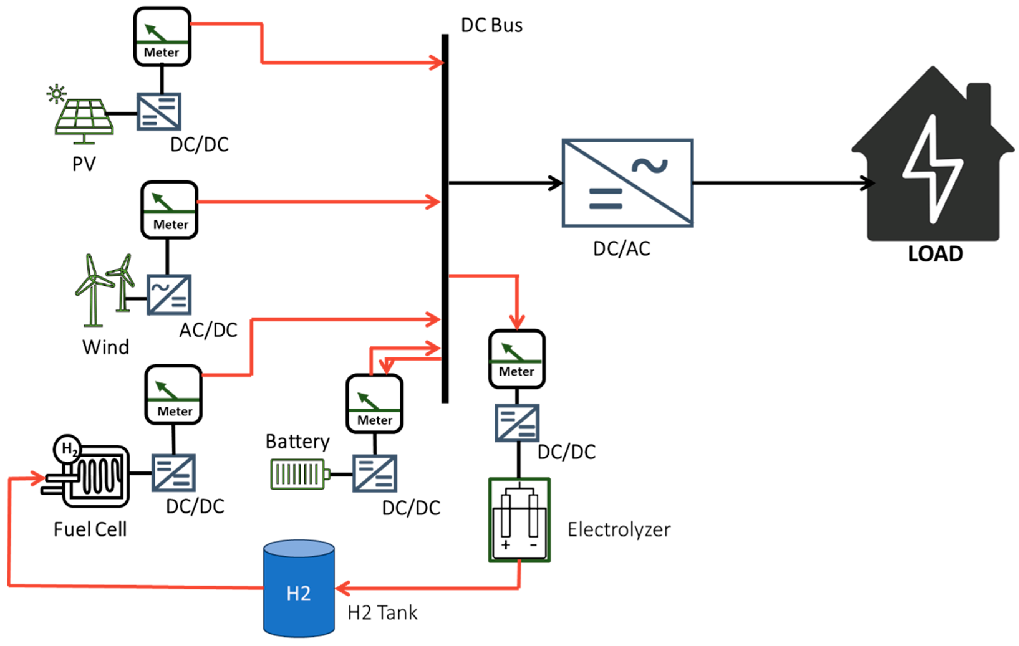
Figure 2.
Load profile and Weather conditions.
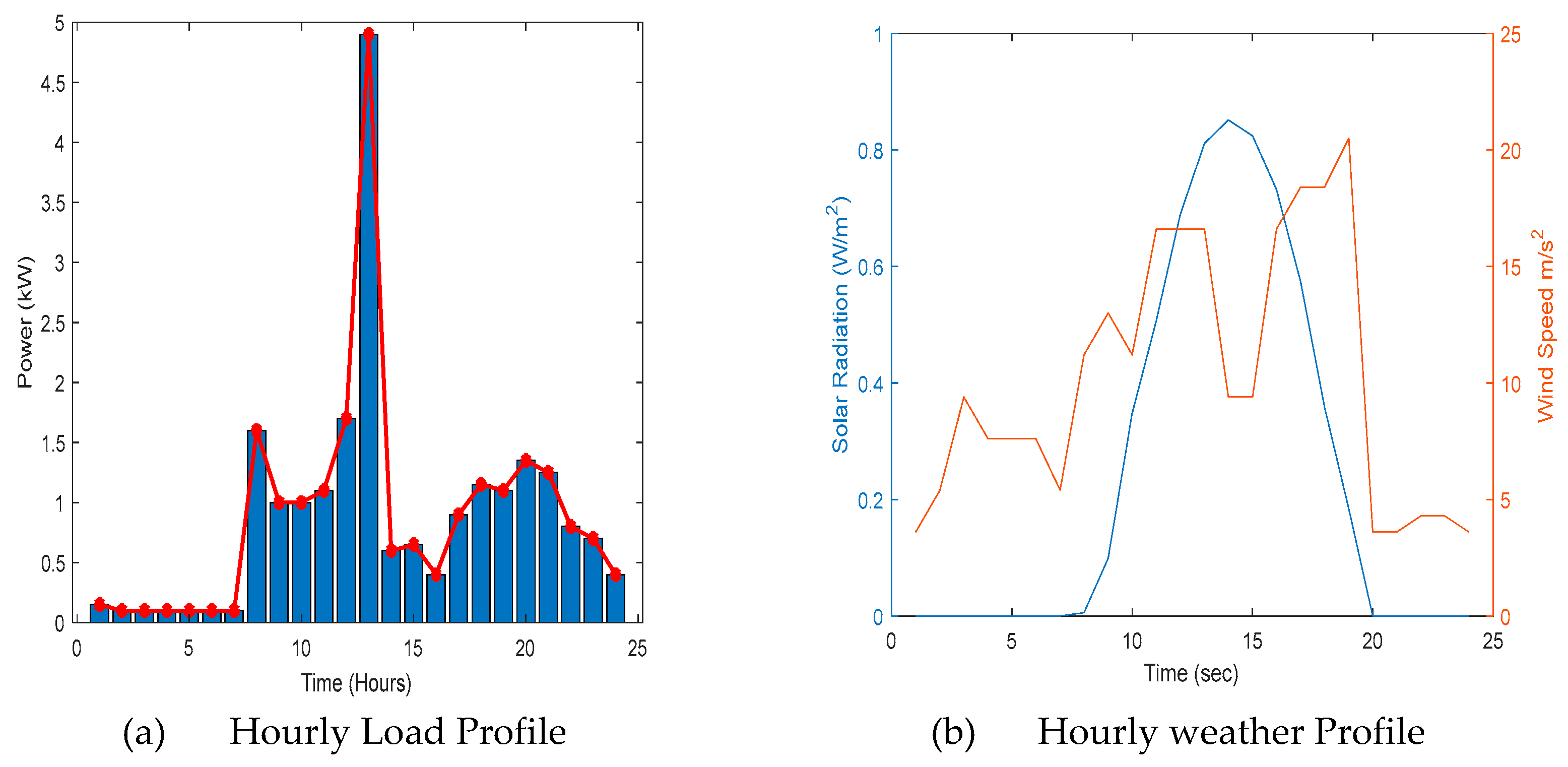
Figure 3.
Modified smell agent optimization flow chart.
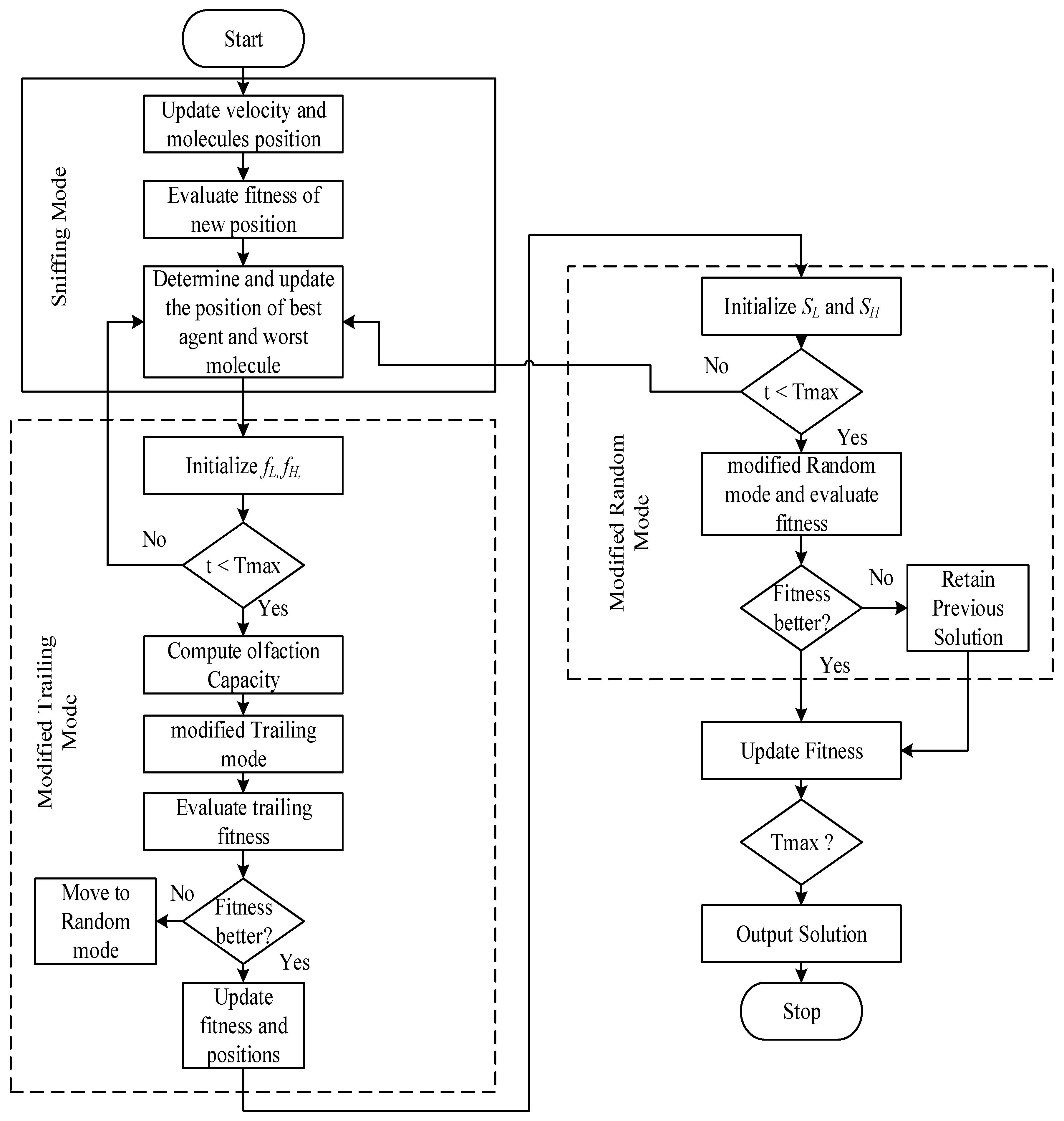
Figure 4.
Flowchart of proposed hybrid energy management system.
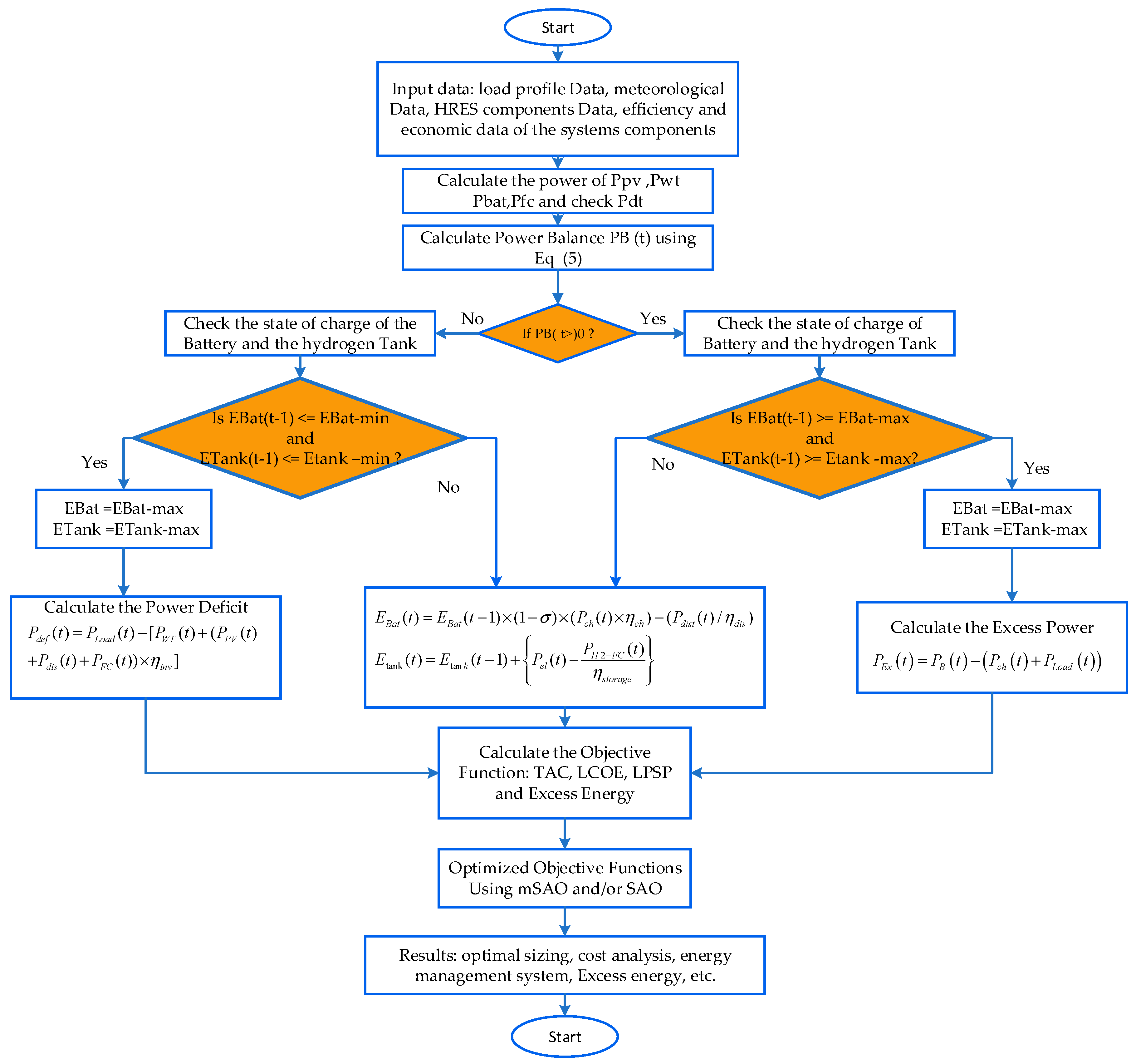
Figure 5.
Convergence (a) SAO on all Configurations (b:) mSAO on all Configurations throughout 100 iterations.
Figure 5.
Convergence (a) SAO on all Configurations (b:) mSAO on all Configurations throughout 100 iterations.
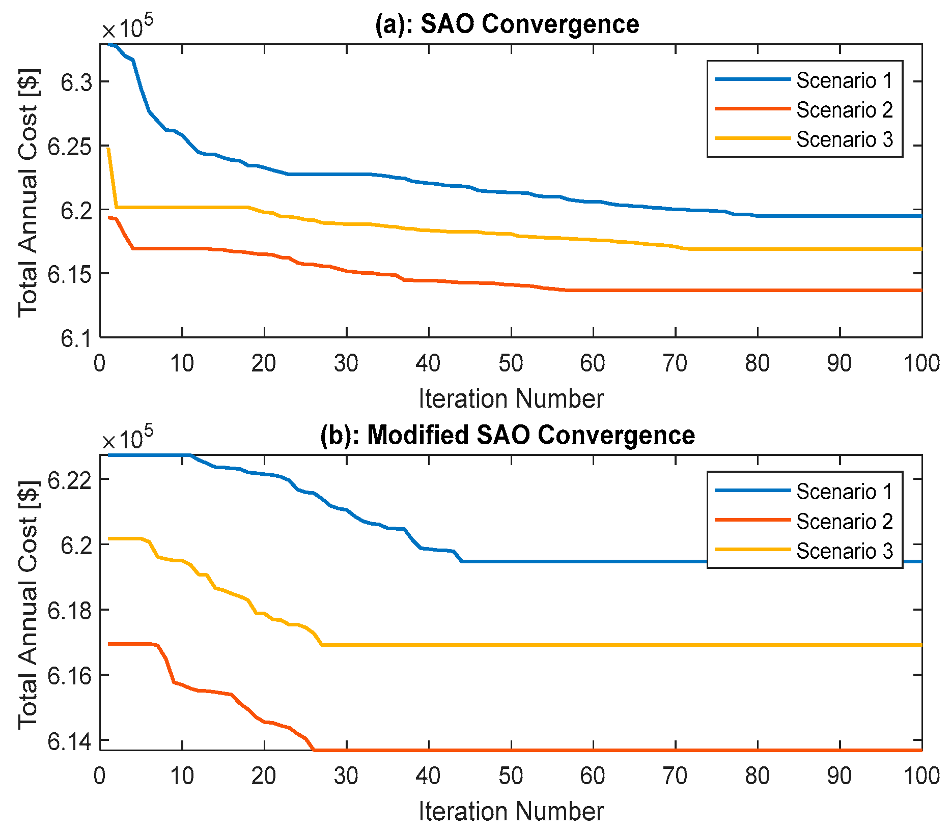
Figure 6.
The convergence of the objective function throughout 100 iterations.
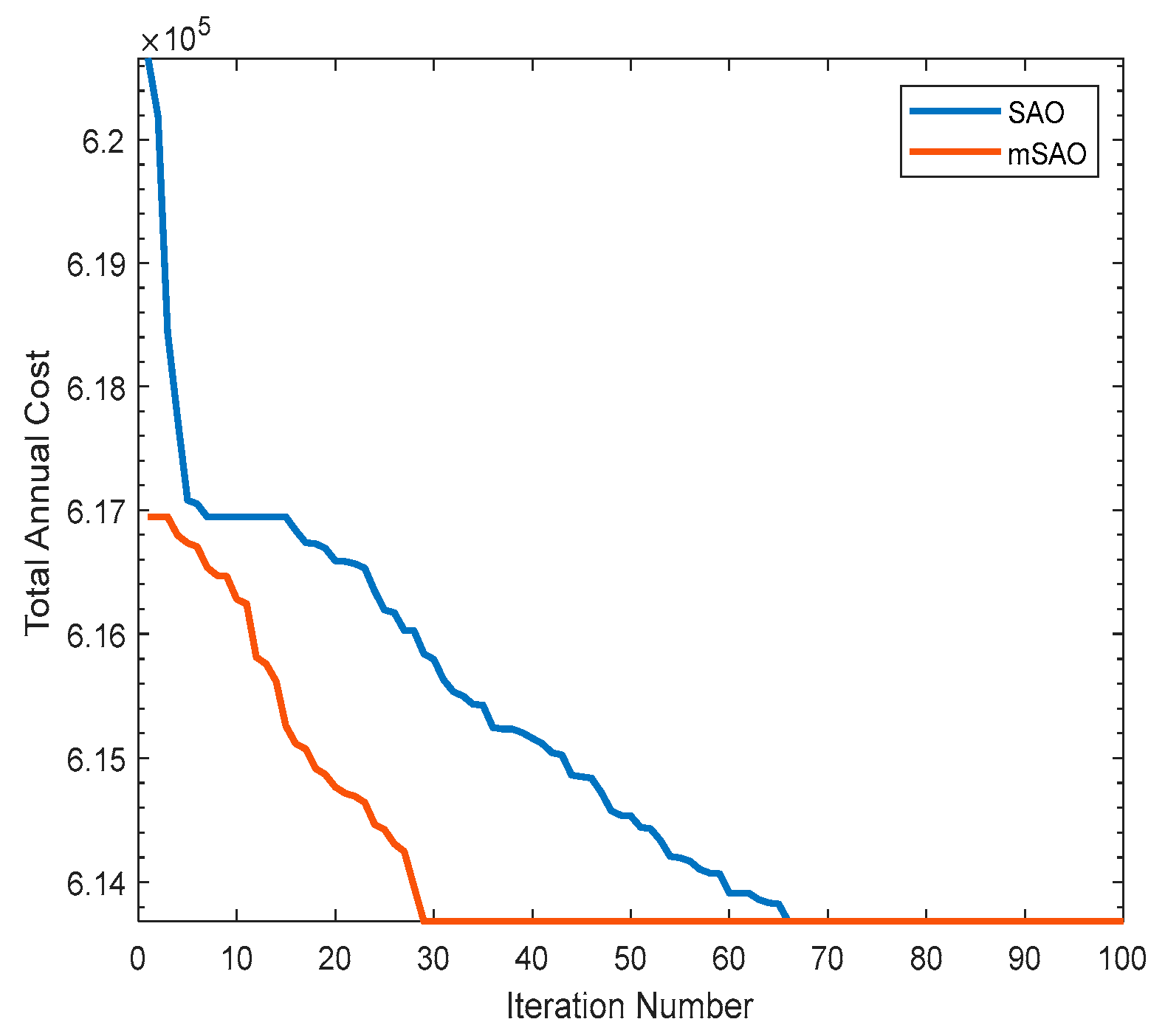
Figure 7.
All 50-Run Total Annual Cost Convergence for the Second Scenario.
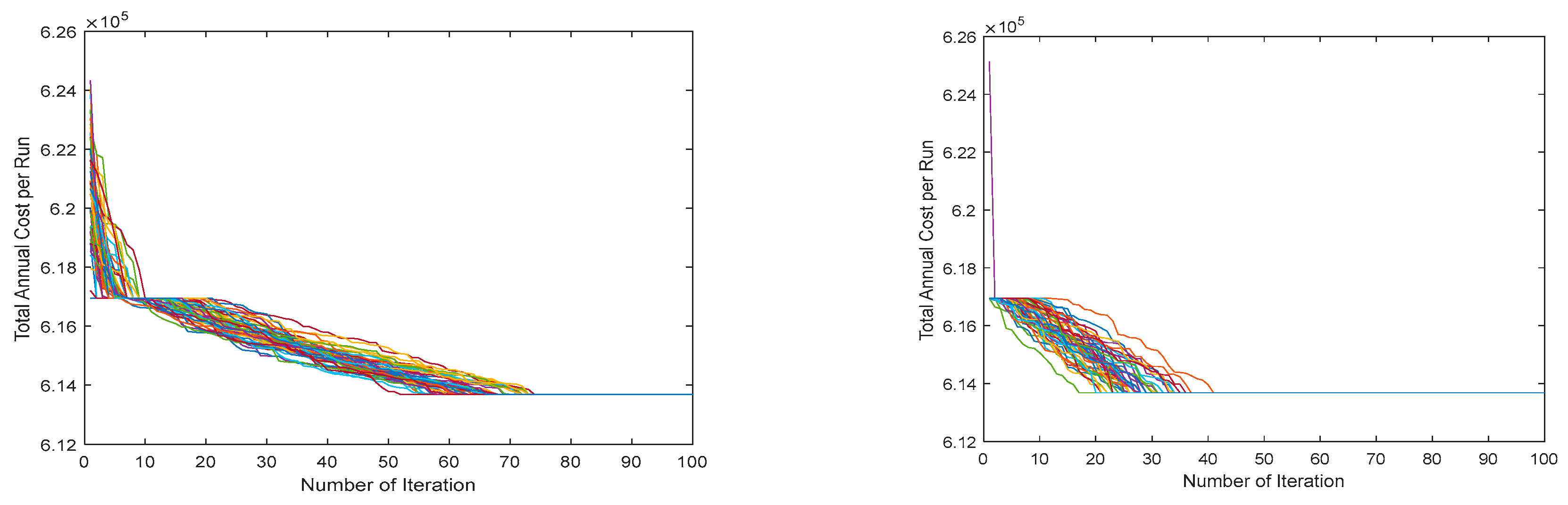
Figure 8.
End value of the objective function on the 50 individual run using SAO and mSAO, (a) PV/WT/Hydrogen /Battery, (b) PV/WT/Battery, (c) PV/WT/Hydrogen.
Figure 8.
End value of the objective function on the 50 individual run using SAO and mSAO, (a) PV/WT/Hydrogen /Battery, (b) PV/WT/Battery, (c) PV/WT/Hydrogen.
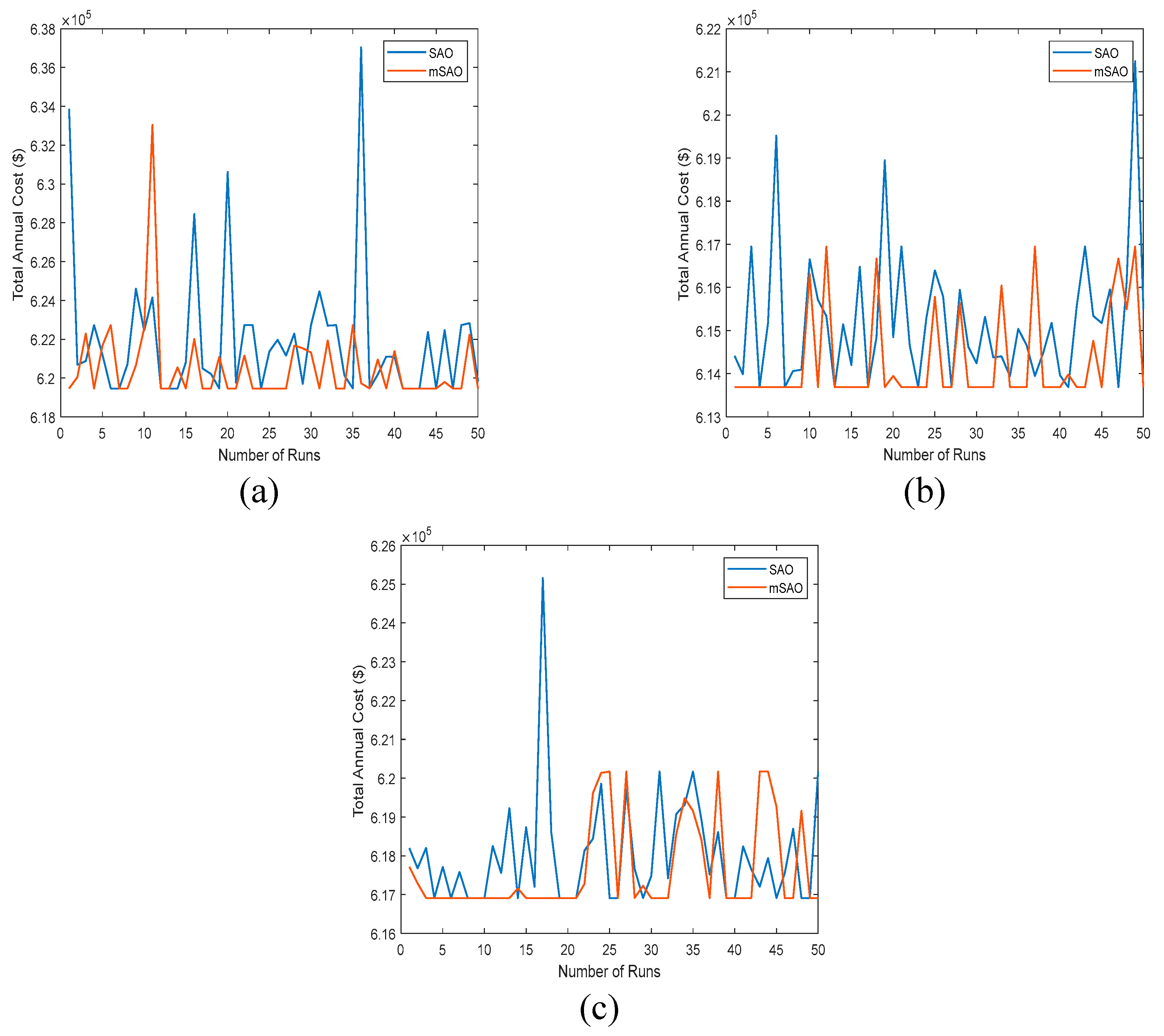
Figure 9.
Comparison curve for all configurations using mSAO of best, (a) LPSP, (b) LCOE, (c) Excess Energy.
Figure 9.
Comparison curve for all configurations using mSAO of best, (a) LPSP, (b) LCOE, (c) Excess Energy.
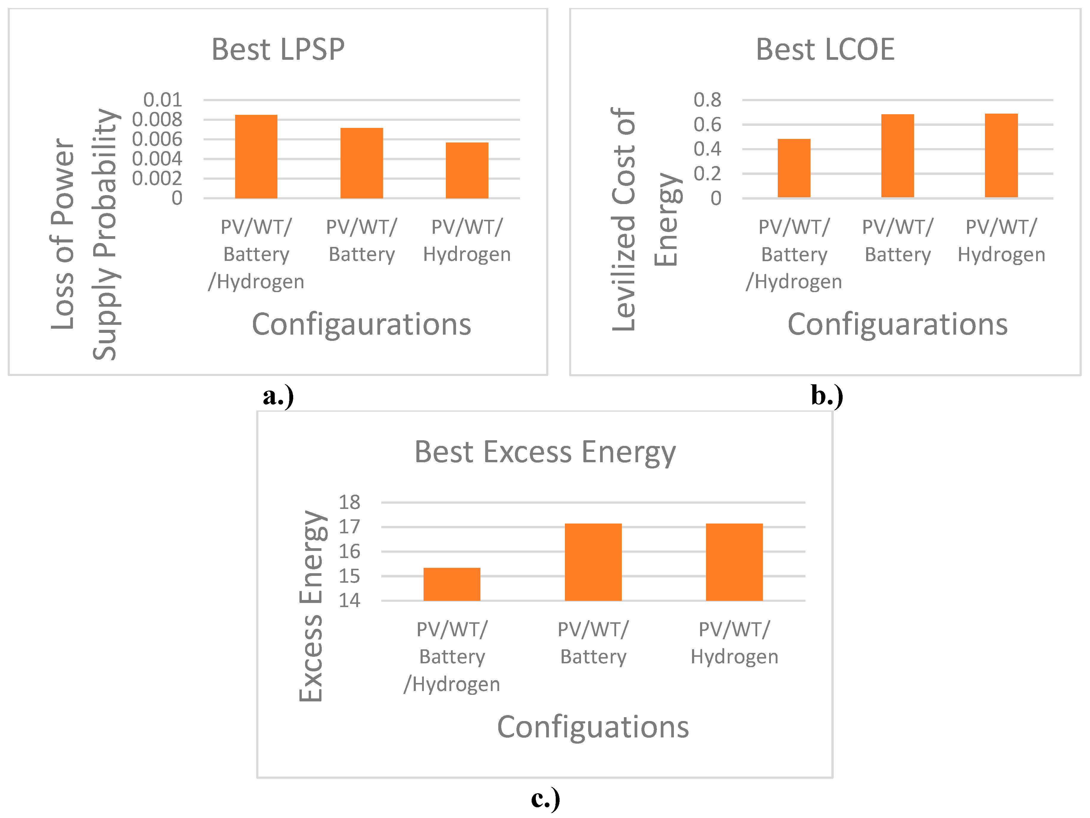
Figure 10.
Breakdown of the TAC obtained by mSAO and SAO for each HRES Component.
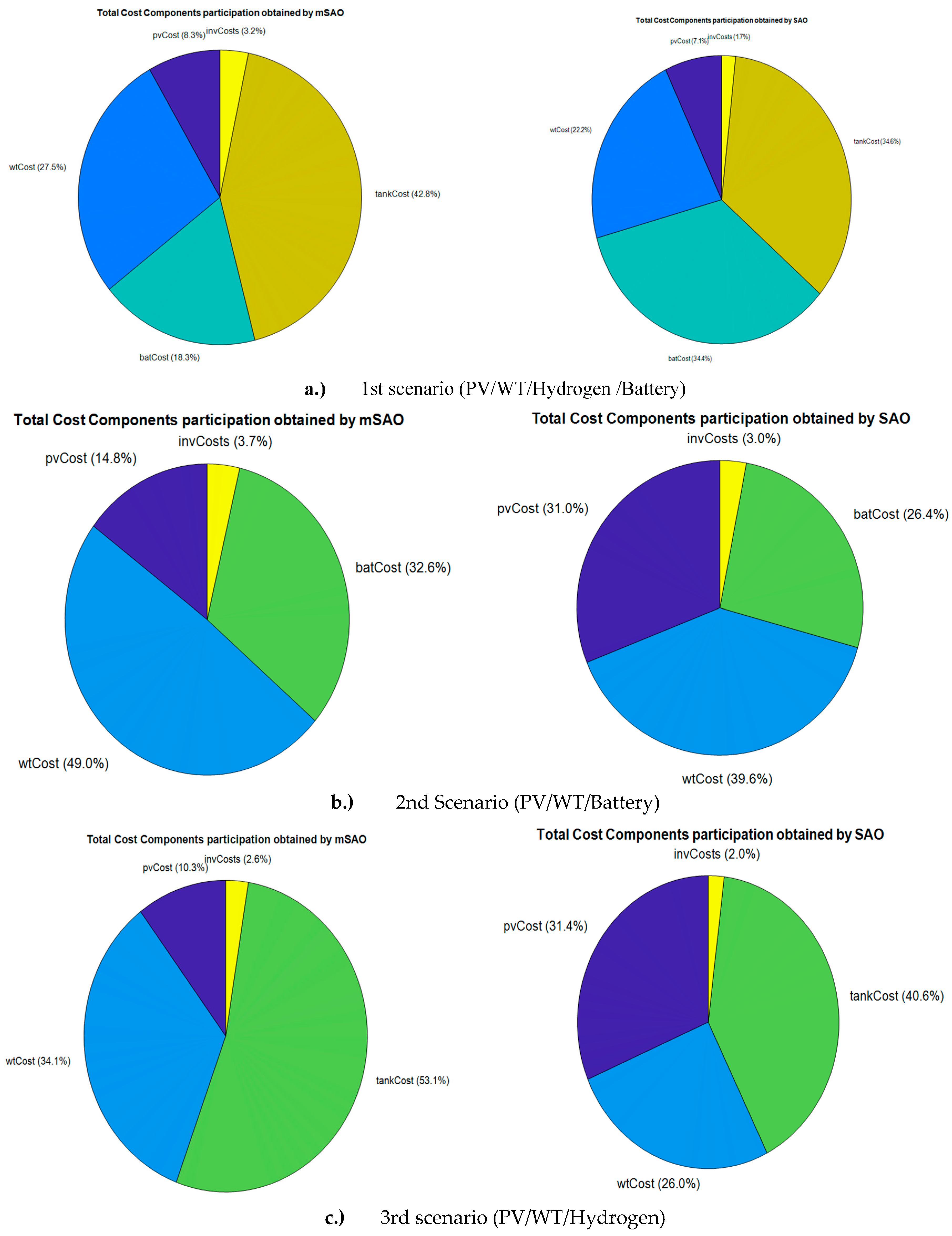
Table 1.
HRES components sizing results.
| Metrics | Scenario 1 (All Components) | Scenario 2 (No Hydrogen) | Scenario 3 (No Battery) | ||||
| SAO | mSAO | SAO | mSAO | SAO | mSAO | ||
| NPV | 8 | 5 | 13 | 5 | 20 | 5 | |
| NWT | 3 | 2 | 2 | 2 | 2 | 2 | |
| NBat | 7 | 2 | 2 | 2 | -- | -- | |
| NTank | 3 | 2 | -- | -- | 2 | 2 | |
| NConv | 5 | 5 | 4 | 4 | 4 | 4 | |
| Total annual cost ($) | Best | 619464.6 | 619464.6 | 613685.5 | 613685.5 | 616910.5 | 616910.5 |
| Average | 622376.4 | 620531.7 | 615217 | 614288.8 | 618031 | 617649.1 | |
| Std | 3.568e-3 | 1.914e-3 | 1.558e-3 | 1.111e-3 | 1.446e-3 | 1.212e-3 | |
| Time (s) | 2.877019 | 4.263277 | 2.958071 | 2.854077 | 2.969879 | 2.851904 | |
Table 2.
Results of the statistical study for the three proposed hybrid configurations using SAO and mSAO algorithms.
Table 2.
Results of the statistical study for the three proposed hybrid configurations using SAO and mSAO algorithms.
| Configuration | Index | SAO | mSAO | |
| PV/WT/ Battery /Hydrogen | LCOE | Best | 0.1845914141 | 0.4827999716 |
| Average | 0.6713710701 | 0.6985542546 | ||
| StD | 0.1153515723 | 0.5468124717 | ||
| LPSP | Best | 0.293372621 | 0.0084838478 | |
| Average | 0.380106609 | 0.0143923633 | ||
| StD | 0.0027696684 | 0.0714469320 | ||
| Excess Energy |
Best | 16.135833379 | 15.340319148 | |
| Average | 16.417603078 | 17.163953138 | ||
| StD | 2.7668380982 | 0.4253515836 | ||
| PV/WT/ Battery | LCOE |
Best | 0.3509501639 | 0.6830423606 |
| Average | 0.6868477489 | 0.7108991366 | ||
| StD | 0.0772454915 | 0.0133358999 | ||
| LPSP |
Best | 0.29337183 | 0.0071446932 | |
| Average | 0.31491137 | 0.0122269890 | ||
| StD | 7.8178237e-04 | 0.0774712029 | ||
| Excess | Best | 13.157611860 | 17.140715003 | |
| Average | 17.078775557 | 17.304232841 | ||
| StD | 0.7833305552 | 0.0774712029 | ||
| PV/WT/ Hydrogen | LCOE | Best | 0.3997548128 | 0.6866308822 |
| Average | 0.6853173504 | 0.7175898792 | ||
| StD | 0.0712544499 | 0.0098690281 | ||
| LPSP | Best | 0.29239547 | 0.0056768049 | |
| Average | 0.31260406 | 0.0104951486 | ||
| StD | 6.4520347e-04 | 0.0714469320 | ||
| Excess Energy |
Best | 14.120005570437 | 17.140715003 | |
| Average | 17.068731687154 | 17.321551245 | ||
| StD | 0.6331719103384 | 0.0567680495 | ||
Disclaimer/Publisher’s Note: The statements, opinions and data contained in all publications are solely those of the individual author(s) and contributor(s) and not of MDPI and/or the editor(s). MDPI and/or the editor(s) disclaim responsibility for any injury to people or property resulting from any ideas, methods, instructions or products referred to in the content. |
© 2025 by the authors. Licensee MDPI, Basel, Switzerland. This article is an open access article distributed under the terms and conditions of the Creative Commons Attribution (CC BY) license (http://creativecommons.org/licenses/by/4.0/).
Copyright: This open access article is published under a Creative Commons CC BY 4.0 license, which permit the free download, distribution, and reuse, provided that the author and preprint are cited in any reuse.


