
Submitted:
14 December 2025
Posted:
15 December 2025
You are already at the latest version
Abstract
Koide's mass formula, originally proposed for charged leptons, has been hypothesized by Carl A. Brannen to also apply to neutrinos. Assuming this hypothesis' validity, two three-dimensional mass models were constructed based on the proposed neutrino masses. This paper demonstrates that the Pontecorvo–Maki–Nakagawa–Sakata (PMNS) matrix can be derived by introducing an intermediate set of hypothetical states, referred to as mass negative eigenstates, which mediate the transformation between mass and flavor eigenstates. This framework naturally reproduces the tribimaximal mixing structure and yields a PMNS matrix with elements close to those obtained using global fits. Neutrino oscillation probability predictions were further compared with results from the Tokai-to-Kamioka (T2K) and Daya Bay collaborations. While the proposed model captures key structural lepton mixing features, a deviation of approximately −3σ in sin2(2θ13) highlights its limitations in terms of reproducing current data. This discrepancy may indicate the involvement of additional mechanisms or physics beyond the current framework. Future theoretical refinements and more precise experimental tests are crucial to assess whether the Koide--Brannen framework can serve as a meaningful step toward a deeper understanding of neutrino phenomenology.
Keywords:
Koide's formula
; θ13
; charge conjugation and parity (CP) violation
; neutrino oscillation
1. Introduction
1.1. Koide’s Mass Formula
1.2. Interpretation by Carl A. Brannen
In 2006, Carl A. Brannen provided an interpretation of Koide’s mass formula [4,5]. Let the masses of ,, and be denoted as , , and , respectively, which are experimentally determined as follows [6]:
According to Brannen, the square root of each mass is expressed as
for This provides a deeper mathematical insight into Koide’s mass formula.
As which follows Brannen’s mass formula, this is used as a normalization factor. Therefore,
1.3. Brannen’s Neutrino Mass Hypothesis
Brannen hypothesized that a similar relationship holds for neutrinos:
Let the masses of , , and be denoted as , , and , respectively. Brannen proposed the following expressions [4,5]:
For ,
where the minus sign appears because this expression evaluates to a negative value.
For , 3,
From these, the neutrino masses are calculated as
1.4. Constructing Two Three-Dimensional (3D) Mass Models
Here, a question arises: While Brannen indicates that the square root of the mass of is negative, what does it mean for the square root of a mass to be negative?
Could it imply that is antimatter? No. The observed should correspond to the positive square root of its mass.
Assuming Brannen’s hypothesis is valid, it is proposed that might be the origin of the rotation in the Pontecorvo–Maki–Nakagawa–Sakata (PMNS) matrix [7]. Based on Brannen’s hypothesis, two three-dimensional (3D) mass models were constructed for neutrinos.
2. Methods
In this study, most of the computations were performed using Microsoft Excel 2021 with its default double-precision arithmetic (approximately 15 significant digits). For plotting and numerical integration, Python was used. In those cases, the Excel outputs were rounded to 12 decimal places and hard-coded into the scripts. Herein, all reported values are rounded to six decimal places for readability; this rounding does not affect the accuracy of the results within reasonable numerical precision.
2.1. Construction of the Neutrino 3D Mass Models
Let the masses of , , and be denoted as , , and , respectively, satisfying
In 3D space, let the origin be ; the radius is defined as
where r represents the radius of a sphere described by .
Points and are defined as
where both lie on the aforementioned sphere. Further, three additional points on the sphere are defined as
The models are constructed in two patterns, based on the square roots of the neutrino masses and the following combinations:
(i) ;
(ii) .
2.1.1. Combination
Vectors and Dot Products
The unit vector (hereafter referred to as the unit vector) is defined as
The following vectors originating from are defined as:
The dot products are calculated as follows:
To align the direction of with the x-axis, , , , and are rotated about the origin in 3D space.
Initial Coordinates
The initial coordinates are expressed as
Rotation in the -Plane
Using and , corresponding to , rotation in the -plane is applied as follows:
Rotation in the -Plane
Using and , corresponding to , rotation in the -plane is applied as follows:
Rotation in the -Plane
Similarly, using and , corresponding to , rotation in the -plane is applied as follows:
For visualization purposes, the z-component of can be set to 0. The x-components of , , and denote , , and , respectively, thus relating each vector with the respective neutrino.
2.1.2. Combination
Vectors and Dot Products
The unit vector is defined as
The vectors originating from are defined as follows:
The dot products are calculated as follows:
To align the direction of with the x-axis, , , , and are rotated about the origin in 3D space.
Initial Coordinates
The initial coordinates are expressed as
Rotation in the -Plane
Using and , corresponding to , rotation in the -plane is applied as follows:
Rotation in the -Plane
Using and , corresponding to , rotation in the -plane is applied as follows:
Rotation in the -Plane
Finally, using and , corresponding to , rotation in the -plane is applied as follows:
The x-components of , , and denote , , and , respectively, thus relating each vector with the respective neutrino.
3. Results
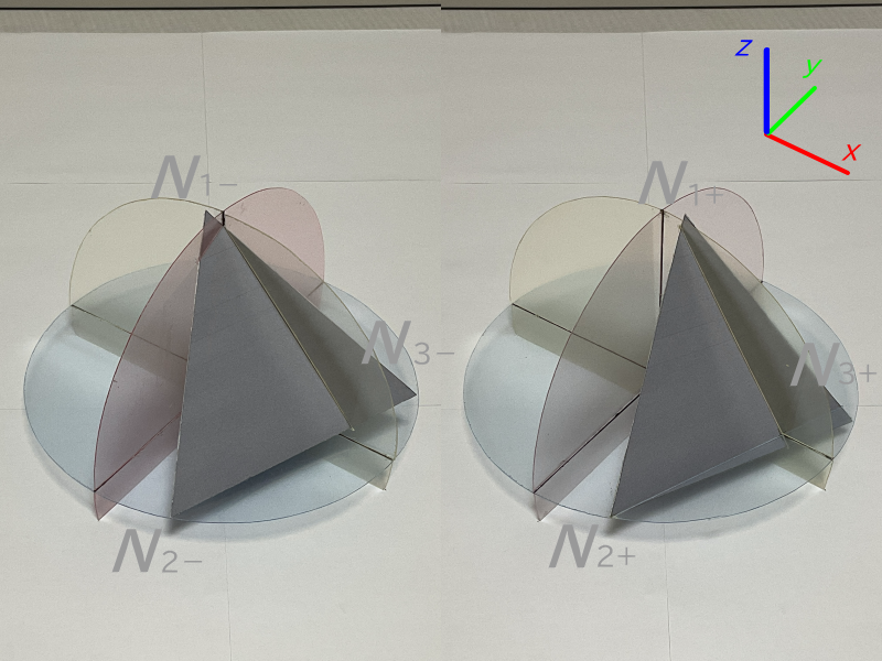
Figure 1 shows the results of the two 3D neutrino mass models.
The relationship between the two models can be expressed as follows:
This simplifies to
Here, .
If the cyclic permutations of the 3–1, 1–2, and 2–3 rotations are considered, the relationship can also be written as
Here, .
4. Discussion
4.1. Correspondence to the Conjugation and Parity (CP) Violation
Each component is extended to a complex value to account for the charge conjugation and parity (CP) violation [8,9]. The extended vectors are given as follows:
which relates each vector with the respective neutrino.
Then, the relationship between the two matrices can be expressed as
This relationship can also be written as
where .
The two states are distinguished as the states in which the square root of the mass of is negative, referred to as mass negative eigenstates , and the states in which it is positive, referred to as mass eigenstates .
By relating each vector with the respective neutrino, the following relation can be written:
Hereafter, the above matrix is denoted as
4.2. Product with the Tribimaximal Mixing Matrix
The tribimaximal mixing matrix [10] is defined by the product of two unitary matrices, as follows:
where , i.e., the complex cube root of unity.
However, does not allow extraction of rotation angles and . Therefore, in this study, the following form of the tribimaximal mixing matrix is adopted:
where
Hereafter, the above matrix is denoted as
This tribimaximal mixing matrix is regarded as a transformation matrix between the mass negative eigenstates and the flavor eigenstates of neutrinos, as follows:
Accordingly, the relationship between the mass and flavor eigenstates can be expressed as
The product of matrices , , and can be approximated as follows:
Could this be interpreted as the PMNS matrix?
The absolute values of each component are as follows:
These values closely match the “Leptonic Mixing Matrix” provided by NuFIT 6.0 [11].
4.3. Neutrino Oscillation
The validity of the derived PMNS matrix depends on whether the neutrino oscillation [12] predictions calculated with it agree with the experimental data.
4.3.1. Probability Calculation
The oscillation probability formula for each neutrino can be derived as follows. Let the flavor states before and after oscillation be and , respectively. Then, the calculation involves the following steps:
(i) Decomposing flavor eigenstate into mass eigenstates using the PMNS matrix;
(ii) Applying phase shifts due to the time evolution of each mass eigenstate; and
(iii) Reconstructing flavor eigenstate from mass eigenstates using the inverse PMNS matrix.
In Step (ii), the phase shift of each (, 2, 3) is shifted by , where depends on the neutrino mass, propagation distance, and energy. In this paper, as the estimated neutrino masses are known, the calculation proceeds in a straightforward manner.
The unit conversion constant for the phase shift is given by
Thus,
where L is the propagation distance and E is the neutrino energy.
In Step (iii), the inverse of the PMNS matrix is required.
Representing the PMNS matrix as
and noting that the PMNS matrix is unitary, its inverse is simply its Hermitian adjoint matrix. Therefore,
The oscillation probability from to , denoted as , is given by
For antineutrinos, the corresponding probability is
or alternatively:
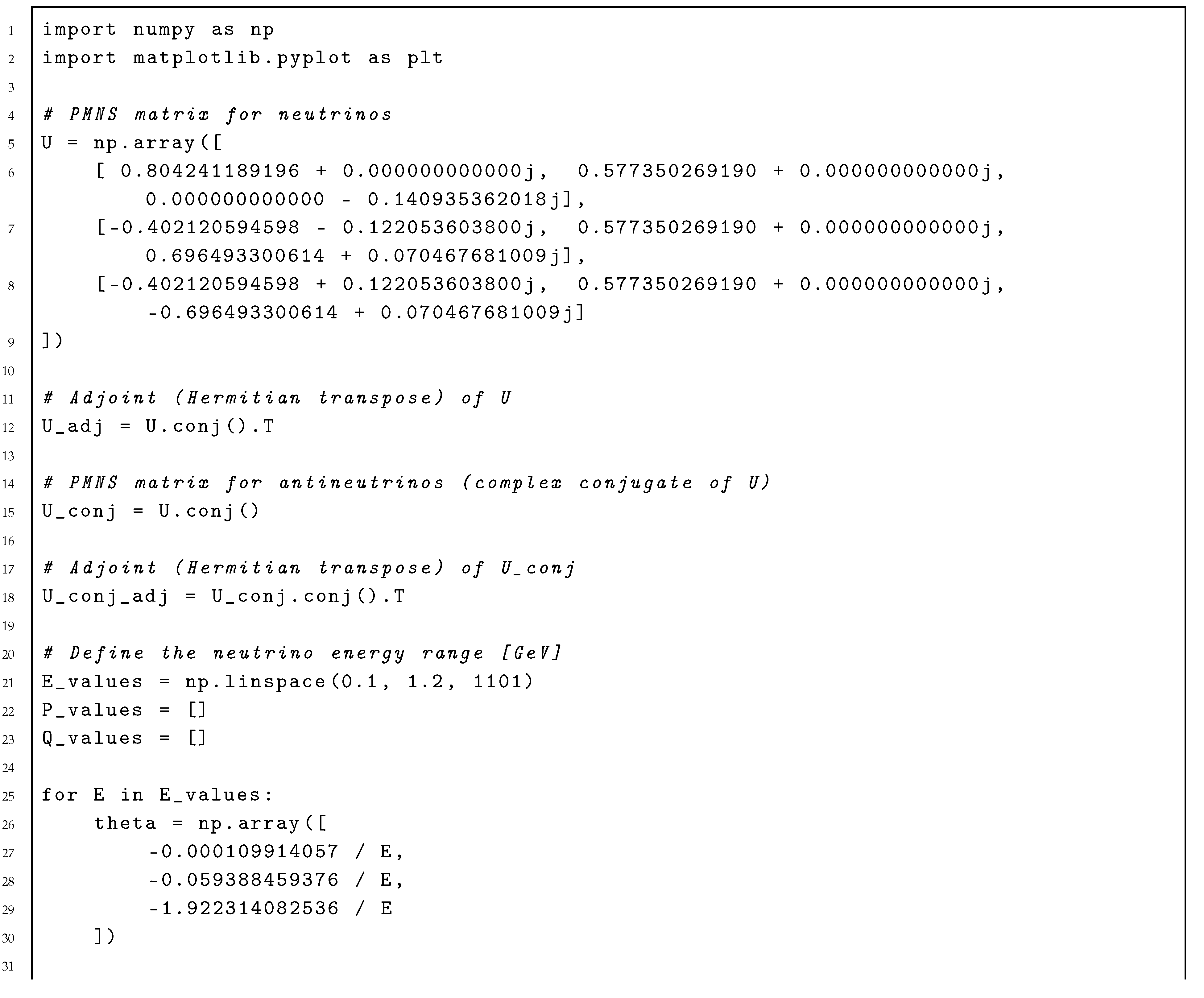
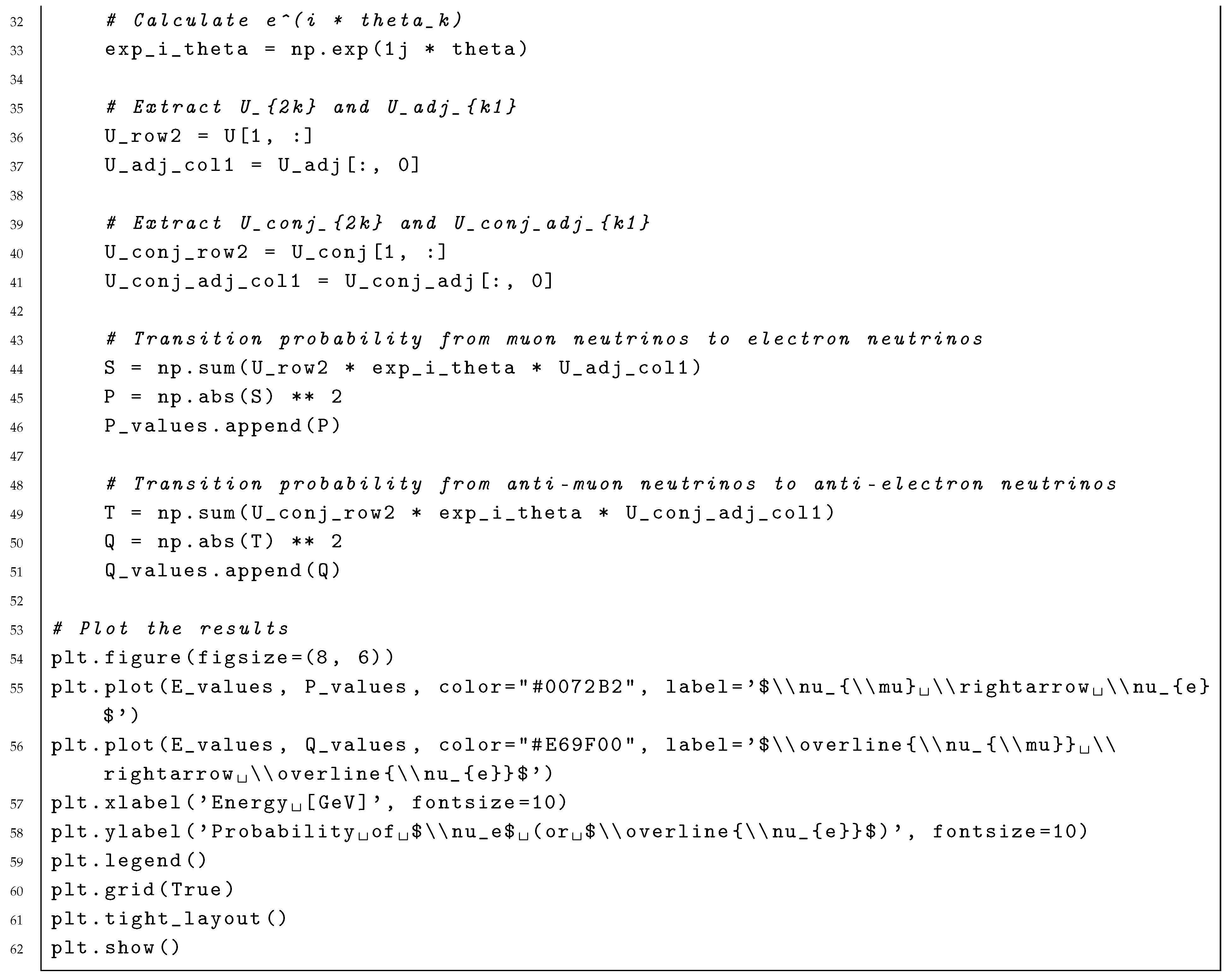
Following the Tokai-to-Kamioka (T2K) [13,14] experimental setup, and were calculated numerically using Python (see Appendix A.1 for more details). When the propagation distance is fixed at , the oscillation probabilities depend on the neutrino energy (Figure 2).
4.3.2. Energy Distribution of the Muon (Anti-)Neutrino Beam
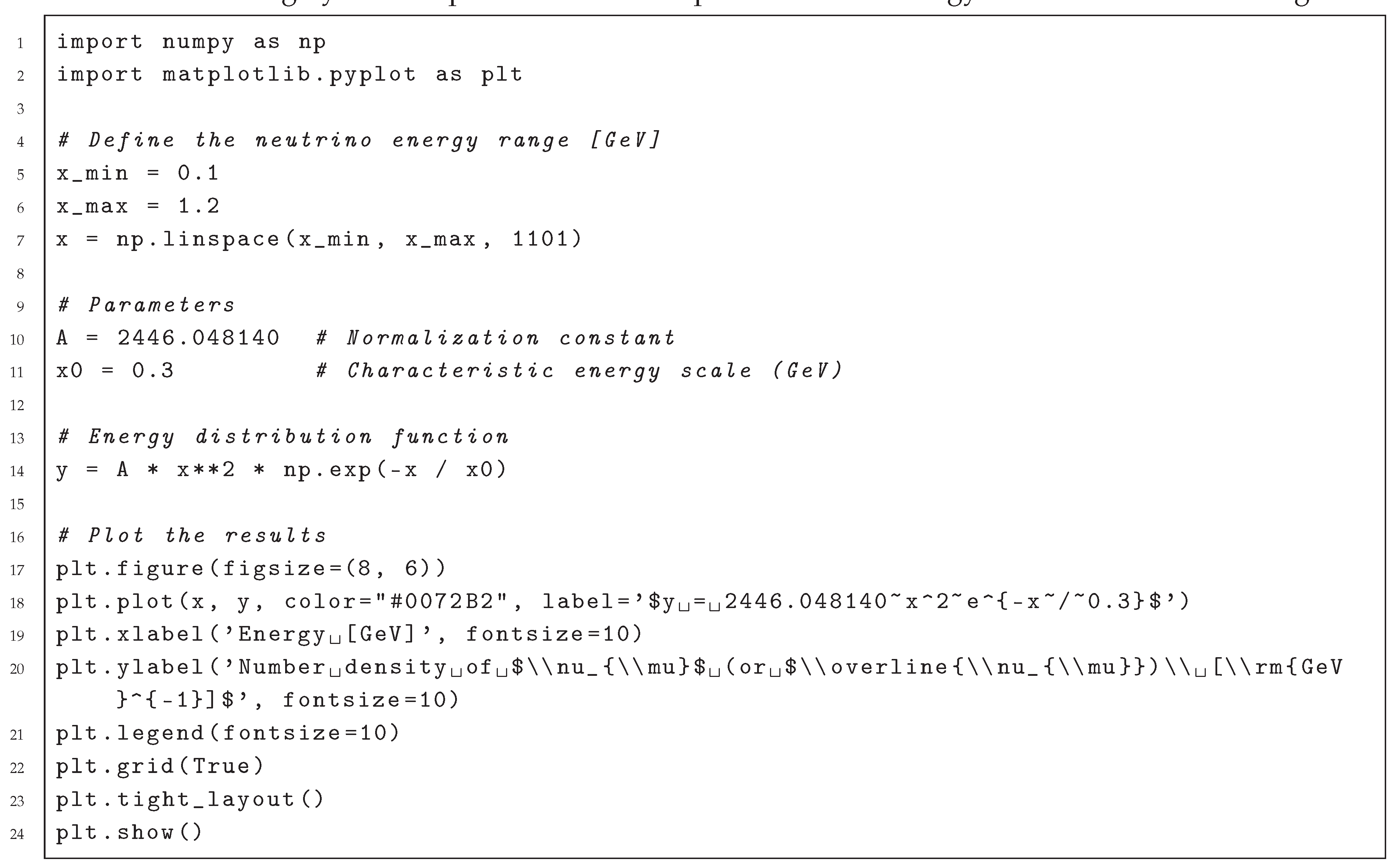
Based on this experimental setup, the emitted (or ) beam energy is not precisely ; instead, it exhibits a spread in its distribution. Although the exact form of the beam energy distribution is unknown, it is assumed to be represented by a function such as
where represents the beam energy and denotes the number density of the emitted (or ). This distribution is shown in Figure 3, where the function peaks at . This distribution was evaluated numerically using Python (see Appendix A.2 for more details).
The expected number of emitted (or ) in the energy range of 0.1–0.2 is given by
4.3.3. Probability Density and Expected Number of (Anti-)Neutrinos
By combining the two functions, the probability density for (or ) was calculated numerically using Python (see Appendix A.3 for more details), as shown in Figure 4. The resulting distribution closely resembles that reported in Figure 3 of Ref. [14].
Integration over the 0.1–0.2 interval yields the following expectations:
For 100 neutrinos, the expected number of events is approximately ; for 100 antineutrinos, the expected number of events is approximately .
4.4. Comparison with Experimental Data and Model Limitations
As can be seen, the expectation for is less than , which is smaller than anticipated.
Therefore, a comparison with experimental data is warranted.
Let the rotation angles in the reordered 1–2, 1–3, and 2–3 rotations be denoted as , , , and , and assume
From the (3,1) element of the matrices, the following are obtained:
which yields
The Daya Bay experiment, as reported by Chen [15], measured the following:
By contrast, the present model yields a deviation of approximately .
This discrepancy indicates that the model, in its current form, is insufficient to fully reproduce the experimental results. Furthermore, this deviation may indicate missing elements in the proposed framework, such as additional interactions, higher-order effects, or new physics beyond the present assumptions. This limitation highlights the need for theoretical refinement. Future experimental and theoretical studies will be essential for clarifying the mechanisms underlying the observed values.
5. Conclusions
In this study, the implications of Koide’s mass formula and Brannen’s neutrino mass hypothesis were examined by constructing two 3D neutrino mass models. The PMNS matrix was shown to be derived by introducing mass negative eigenstates as intermediate states linking the mass and flavor eigenstates. This approach successfully reproduces the tribimaximal mixing structure and yields a PMNS matrix with elements that closely resemble those obtained in global analyses.
Despite some encouraging results, when applied to oscillation observables, the proposed model predicts , which deviates from the Daya Bay measurement by approximately . This discrepancy highlights the limitations of the proposed framework and points to missing ingredients—additional interactions, higher-order effects, or new physics beyond the assumptions considered in this study.
Acknowledgments
The author would like to express his sincere gratitude to Carl A. Brannen for his insightful comments and suggestions during the preparation of this manuscript. The author would also like to acknowledge Editage (www.editage.com) for their support in manuscript preparation.
Appendix A
Appendix A.1. Code for Figure 2
The following Python script was used to compute the oscillation probabilities shown in Figure 2.
Appendix A.2. Code for Figure 3
The following Python script was used to compute the beam–energy distribution shown in Figure 3.
Appendix A.3. Code for Figure 4
The following Python script was used to compute the (or ) probability density shown in Figure 4 by combining the two functions.
References
- Koide, Y. Fermion-boson two body model of quarks and leptons and Cabibbo mixing. Lettere al Nuovo Cimento 1982, 34(7), 201–206. [Google Scholar] [CrossRef]
- Koide, Y. A fermion-boson composite model of quarks and leptons. Physics Letters B 1983, 120(1–3), 161–165. [Google Scholar] [CrossRef]
- Quark masses and Cabibbo angles. Physics Letters B 78(4), 459–461. [CrossRef]
- Brannen, C. A. The lepton masses. Brannen Works. 2006. Available online: https://brannenworks.com/MASSES2.pdf.
- Brannen, C. A. Spin path integrals and generations. Foundations of Physics 2010, 40, 1681–1699. [Google Scholar] [CrossRef]
- Particle Data Group Collaboration. Review of particle physics. Physical Review D 2024, 110, 030001. [Google Scholar] [CrossRef]
- Remarks on the unified model of elementary particles. Progress of Theoretical Physics 28(5), 870–880. [CrossRef]
- Evidence for the 2π decay of the K20 meson. Physical Review Letters 13(4), 138–140. [CrossRef]
- CP-violation in the renormalizable theory of weak interaction. Progress of Theoretical Physics 49(2), 652–657. [CrossRef]
- Tri-bimaximal mixing and the neutrino oscillation data. Physics Letters B 530(1–4), 167–173. [CrossRef]
- NuFit-6.0: Updated global analysis of three-flavor neutrino oscillations. Journal of High Energy Physics 2024, 12, 216. [CrossRef]
- Pontecorvo, B. Inverse beta processes and nonconservation of lepton charge. Zhurnal Éksperimental’noĭ i Teoreticheskoĭ Fiziki;Soviet Physics JETP Reproduced and translated in. 1958, 34 7(1), 247–249 172–173. [Google Scholar]
- T2K Collaboration. Measurement of neutrino oscillation parameters from the T2K experiment. Physical Review Letters 2017, 118, 151801. [Google Scholar] [CrossRef]
- T2K Collaboration. Search for CP violation in neutrino oscillations. arXiv 2023, arXiv:2310.11942. [Google Scholar]
- Chen, Z. Latest results from Daya Bay using the full dataset. arXiv 2023, arXiv:2309.05989. [Google Scholar] [CrossRef]
Figure 1.
Results of the two 3D neutrino mass models.
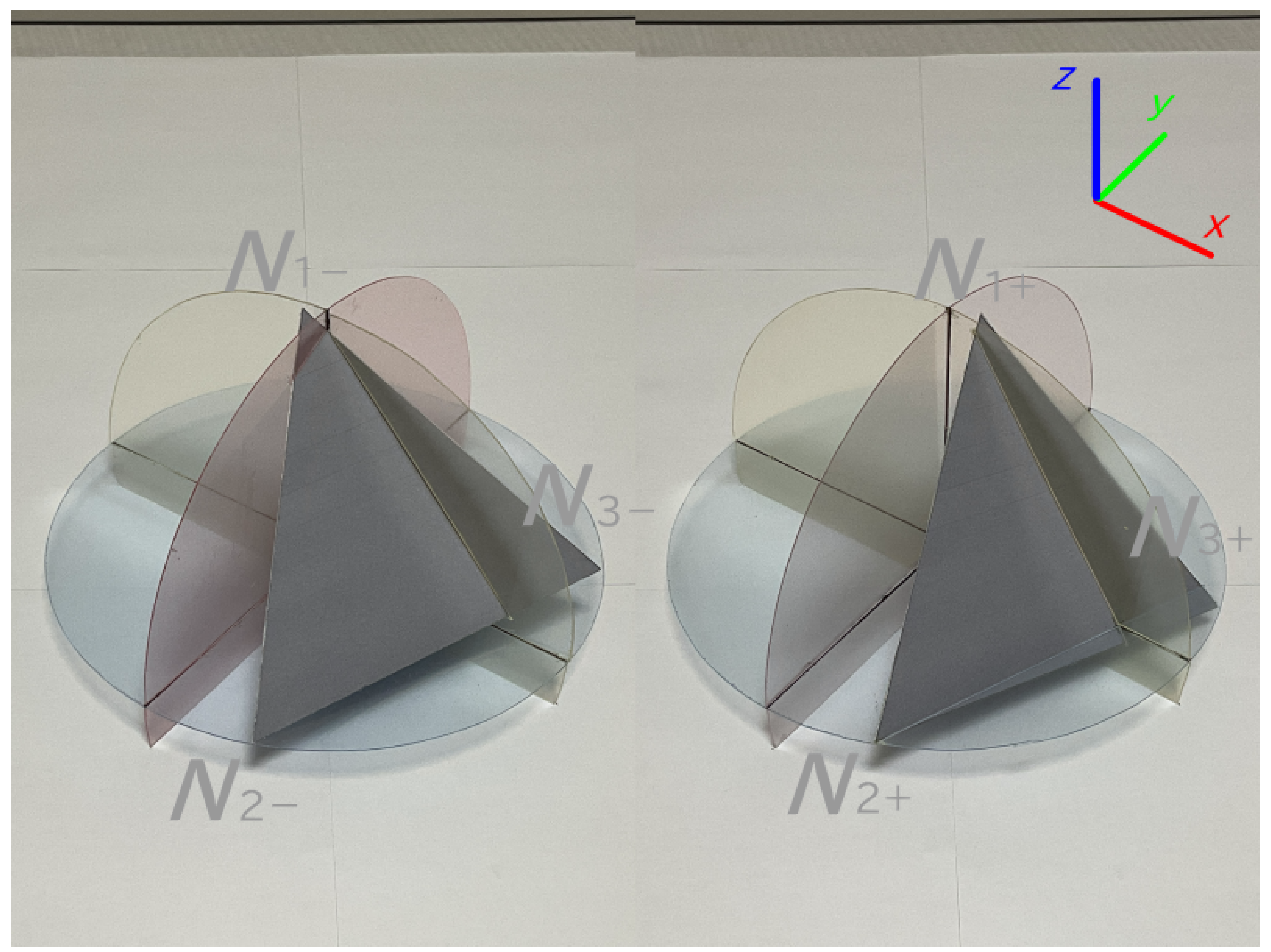
Figure 2.
Relationship between the neutrino energy and oscillation probability.
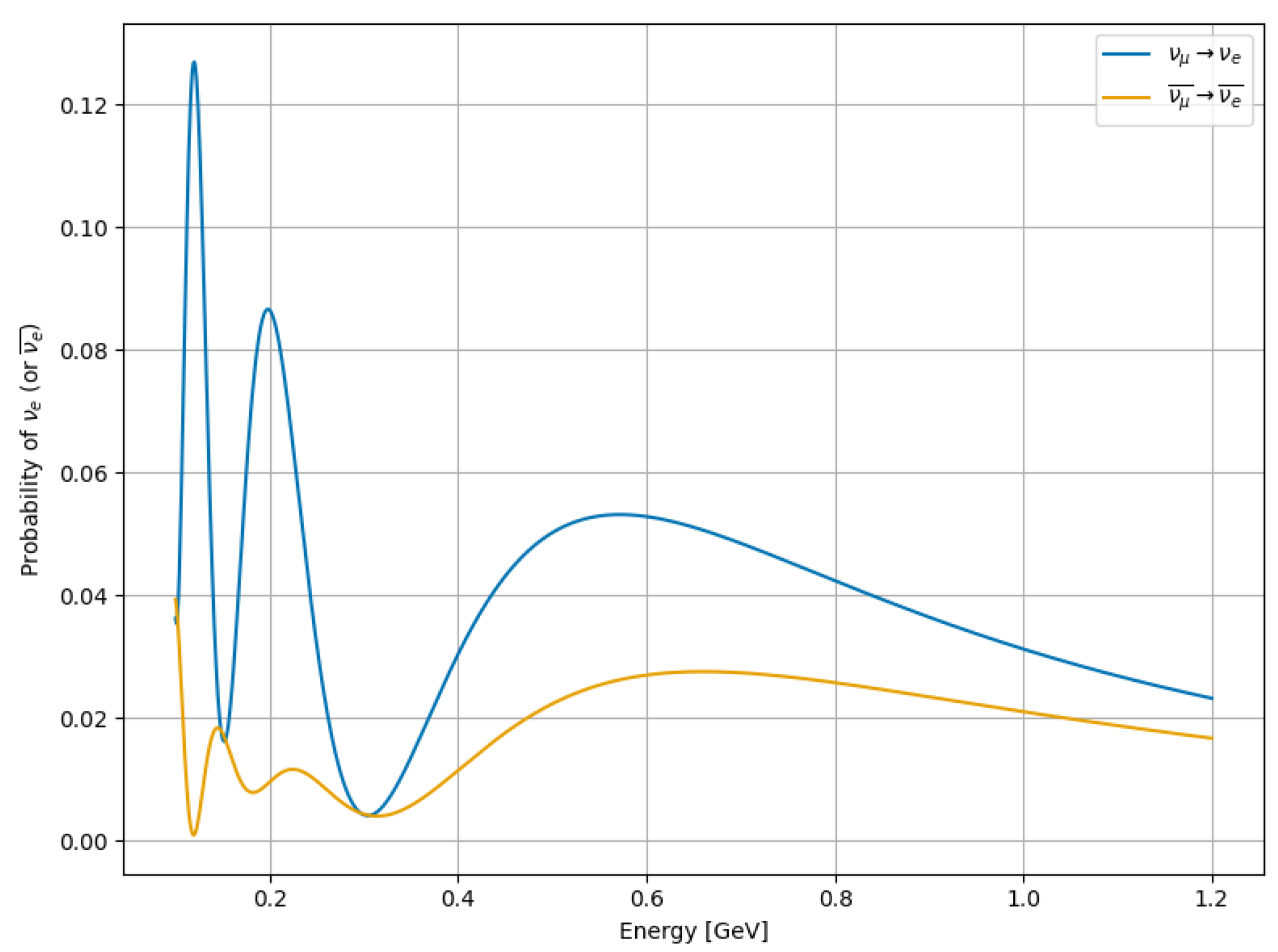
Figure 3.
Relationship between the neutrino beam energy and the number density of (or ).
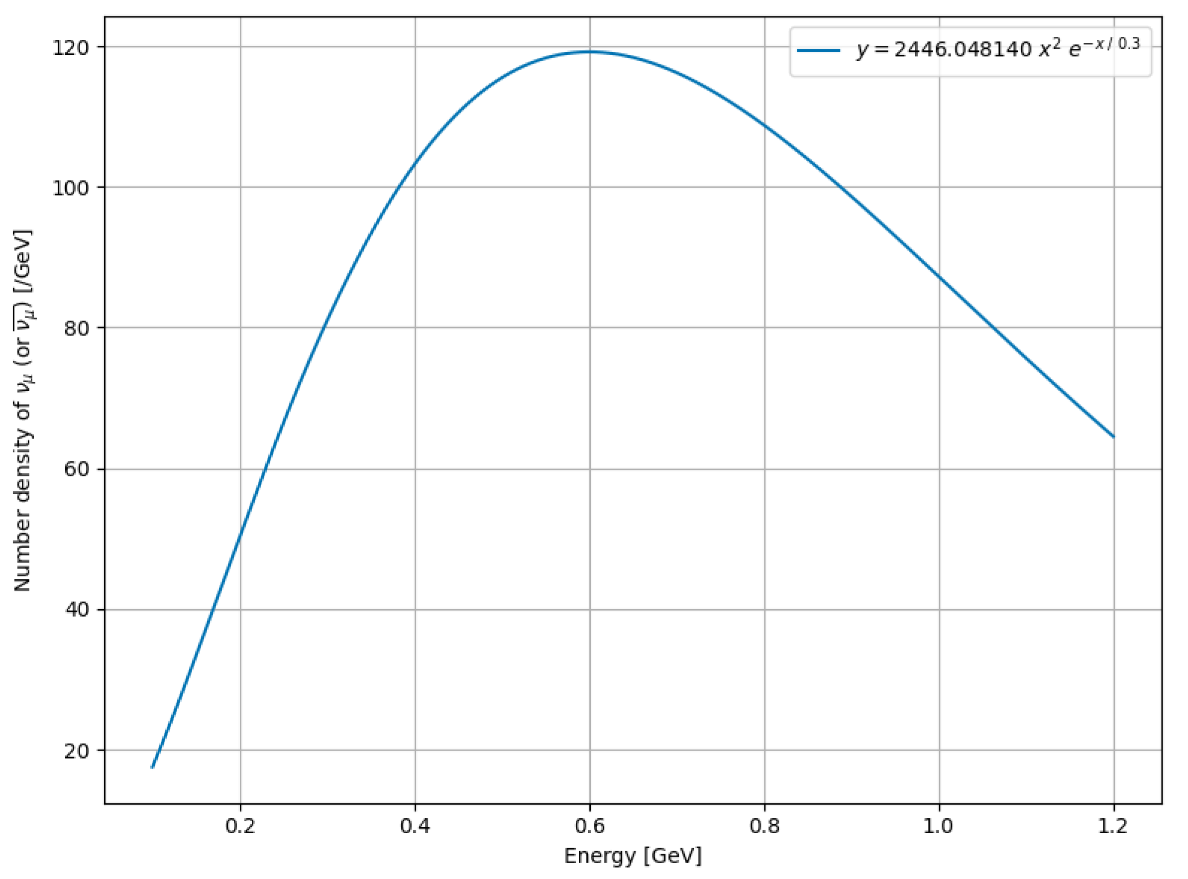
Figure 4.
Relationship between the neutrino energy and the probability density of (or ).

Disclaimer/Publisher’s Note: The statements, opinions and data contained in all publications are solely those of the individual author(s) and contributor(s) and not of MDPI and/or the editor(s). MDPI and/or the editor(s) disclaim responsibility for any injury to people or property resulting from any ideas, methods, instructions or products referred to in the content. |
© 2025 by the authors. Licensee MDPI, Basel, Switzerland. This article is an open access article distributed under the terms and conditions of the Creative Commons Attribution (CC BY) license (http://creativecommons.org/licenses/by/4.0/).
Copyright: This open access article is published under a Creative Commons CC BY 4.0 license, which permit the free download, distribution, and reuse, provided that the author and preprint are cited in any reuse.


