
Submitted:
14 April 2025
Posted:
16 April 2025
You are already at the latest version
Abstract
The semi-Mediterranean (SM) and semi-arid (SA) regions, exemplified by the Kurdo-Zagrosian forests in western Iran and northern Iraq, have experienced frequent wildfires in recent years. This study has proposed a modified Non-Negative Matrix Factorization (NMF) method for detecting fire-prone areas using satellite-derived data in SM and SA forests. The performance of the proposed method was then compared with three other already proposed NMF methods: Principal Component Analysis (PCA), K-means, and IsoData. NMF is a factorization method renowned for performing dimensionality reduction and feature extraction. It imposes non-negativity constraints on factor matrices, enhancing interpretability and suitability for analyzing real-world datasets. Sentinel-2 imagery, the Shuttle Radar Topography Mission (SRTM) Digital Elevation Model (DEM), and the Zagros Grass Index (ZGI) from 2020 were employed as inputs and validated against post-2020 burned area derived from the Normalized Burned Ration (NBR) index. Results demonstrate NMF’s effectiveness in identifying fire-prone areas across large geographic extents typical of SM and SA regions. The results also revealed that when elevation was included, NMF_L1/2 sparsity offered the best outcome among the used NMF methods. In contrast, the proposed NMF method provided the best results when only Sentinel 2 bands and ZGI were used.
Keywords:
fire susceptibility
; NMF
; semi-Mediterranean
; semi-arid
; ZGI
; machine learning
1. Introduction
Forest fires’ rising frequency and severity have emerged globally as a critical issue fueled by natural factors and human activities. Extreme weather events, shifts in land use, and rapid urban development are crucial contributors to this growing problem, exacerbating the risk of wildfires [1,2,3,4]. In 2021, wildfires caused the global loss of approximately 7.02 million hectares of tree cover [5]. Climate change has exacerbated these incidents through rising temperatures, decreased precipitation, and more frequent droughts. In contrast, human activities such as deforestation and land-use changes have further contributed to this escalation. These effects are particularly severe in vulnerable regions like the Semi-Mediterranean (SM) and Semi-Arid (SA) forests of the Kurdo-Zagrosian mountains in western Iran and northern Iraq [6,7,8]. The consequences of forest fires extend beyond immediate environmental damage; they contribute to global carbon emissions and disrupt ecosystems, leading to soil degradation, erosion, loss of microfauna and flora, and the deterioration of water quality [9].
In response to these challenges, early identification of fire-prone areas has become increasingly crucial for effective risk mitigation. Forest Fire Susceptibility Mapping (FFSM) is vital in identifying fire-prone areas or areas at high risk of wildfires, enabling better ecological management and biodiversity conservation [10,11,12]. Such map-ping efforts are significant for regions like the Kurdo-Zagrosian mountains, where human activity and climate change are constantly threatened. By accurately mapping fire-prone zones, FFSMs help decision-makers prioritize resources, reduce vulnerability-ties, and implement preventive measures, ensuring long-term ecosystem health. These efforts rely on factors such as vegetation cover, temperature, humidity, rainfall, wind speed, proximity to roads and water bodies, elevation, slope, land use patterns, and the Topographic Wetness Index (TWI) [13,14,15,16].
Technological advances, particularly in combining Geographic Information Systems (GIS) with Remote Sensing (RS) data/techniques, have revolutionized the development of FFSMs, enabling more precise identification of fire-prone areas. Additionally, ensemble models, which combine the strengths of multiple algorithms, have shown superior accuracy in predicting fire susceptibility [17,18,19]. Studies have demonstrated that these models applied across regions like Gangwon-do in South Ko-rea and the Chaloos Rood watershed in Iran have yielded highly accurate predictions by integrating topography, climate, and human activity [20,21]. Beyond this, integrating geospatial and RS data has allowed researchers to account for various factors that influence wildfire susceptibility, such as temperature, land use, proximity to roads, slope, and vegetation cover [13,22]. Cloud-based platforms like Google Earth Engine (GEE) have facilitated the development of FFSMs by providing powerful processing capabilities for large-scale data analysis. Studies employing GEE, such as those conducted by [23], have achieved highly accurate fire susceptibility predictions for India, with Area Under the Curve (AUC) values exceeding 90%.
On the other hand, several studies have focused on classifying various land features and vegetation types for mapping fire-prone areas using only reflectance data from satellite sources, bypassing topographic features like slope, aspect, and distance from roads [4,24,25,26,27]. These models primarily utilize spectral indices from satellite imagery, such as the Normalized Difference Vegetation Index (NDVI), Enhanced Vegetation Index (EVI), Live Fuel Moisture Content (LFMC), and Zagros Gras Index (ZGI) derived from RS data [4,8,24,25,26,27,28,29]. These indices can capture vegetation’s health, moisture content, and stress, all critical factors in fire susceptibility.
Unsupervised techniques, such as Principal Component Analysis (PCA), K-means clustering, IsoData, and Non-negative Matrix Factorization (NMF), have shown significant potential in studying environmental studies [30,31,32]. PCA, K-means clustering, and IsoData are widely used unsupervised techniques that facilitate the analysis of complex datasets. PCA is a dimensionality reduction method that transforms correlated variables into a smaller set of uncorrelated variables, known as principal components, which capture the most variance in the data [33,34]. On the other hand, K-means and IsoData clustering partition the data into K distinct clusters based on feature similarity, making it effective for identifying patterns within large [35]. Collectively, these methods are instrumental in extracting meaningful information from RS data, supporting applications such as land cover classification and environmental monitoring [35,36]. Moreover, NMF is a dimensionality reduction method that breaks down data into non-negative components and their associated weights. This approach provides interpretable results, as the non-negativity constraint leads to distinct, additive parts, making it ideal for applications like image processing and spectral unmixing, where understanding individual, meaningful components is essential [37,38].
Satellite-based models and indices like NDVI, EVI, LFMC, and ZGI leverage spectral data to assess vegetation characteristics, relying on pre-existing knowledge of biomass and land surface properties while often excluding terrain factors such as slope or proximity to roads. These models evaluate vegetation’s health and stress through satellite band analysis [24,25,26,27,28,29].
Unsupervised methods such as PCA, K-means clustering, and IsoData enable automatic detection of patterns in data, which is widely applied in environmental studies and landcover mapping for dimensionality reduction and clustering [39,40]. NMF, though primarily employed for hyperspectral data reduction and unmixing [41], offers unique benefits through interpretable non-negative components [38,41] yet remains less explored in mapping fire susceptibility, highlighting the potential for further research. NMF is particularly suited for post-fire analysis due to its non-negativity constraint, which aligns with the physical properties of spectral reflectance. Its ability to decompose mixed pixels—common in burned landscapes—into interpretable, additive components makes it effective for burn severity mapping [42]. Unlike supervised classifiers, NMF does not require labeled training data, making it advantageous for rapid post-fire assessment.
Besides proposing a modified NMF method, sparse and endmember-independent NMF (SEI-NMF), this study aims to perform a comparative analysis of the latest and three other already developed NMF methods (Basic or Standard NMF, L1 Sparsity, and L1/2 Sparsity) in FSSM regarding other advanced techniques such as PCA, K-means, and IsoData, to evaluate how these unsupervised methods can predict fire-prone in SM and SA area of Kurdo-Zagrosian region, using only satellite-derived data. By extracting features from these images, the study aims to create new satellite-based layers that enhance fire susceptibility understanding, moving beyond the traditional reliance on the NDVI for vegetation representation. Including the ZGI factor accounts for phenological characteristics and enriches the dataset with ecological insights, providing a more comprehensive approach to fire risk assessment.
2. Materials and Methods
2.1. Study Area
The study focuses on the SA and SM climate regions, particularly the forests of Marivan and Sarvabad in Kurdistan Province, western Iran, which have faced numerous wildfires over the past decades (see Figure 1) [8].
Fires typically begin in late May, driven by the accumulation of dry grass species, and persist until the onset of autumn rains. These forests are located between 750 and 1,700 meters above sea level (a.s.l.), neighboring different shrub species [43]. Grass species, highly flammable and widespread, further increase fire vulnerability, especially during the dry summer months, when most of these species dry out, contributing to fire susceptibility [8]. These forests are located near the Iraq border, between longitudes 45°57′50″E and 46°46′41″E and latitudes 35°1′1″N and 35°49′51″N [8]. Marivan sits at an average elevation of 1,287 meters within the northern Zagros mountain range, featuring mountainous terrains and valleys [8]. The region’s SM climate brings cold winters and hot summers, with annual precipitation of approximately 991 mm. The vegetation, predominantly Brant’s oak (Quercus brantii) and Crataegus pontica and Pistacia atlantica, covers dense and semi-dense forests, rangelands, and pastures [44,45]. These areas have experienced numerous fires in recent decades, highlighting the urgent need for studies to address the issue [8].
2.2. Data Sources
The data used in this study are presented in Table 1. Sentinel-2 multispectral imagery, spanning 2020 to 2023, was obtained from the European Space Agency’s (ESA) Copernicus archive via GEE [46]. The elevation data was derived from the Shuttle Radar Topography Mission (SRTM) Digital Elevation Model (DEM) at 30-meter resolution, later resampled to 10 meters using GEE to meet the resolution of the Sentinel-2 data to avoid scaling biases [47]. All datasets were processed within the Universal Transverse Mercator (UTM) coordinate system, Zone 38N (EPSG:32638). Additionally, the ZGI was calculated from the Sentinel-2 imagery [2].
2.3. C. Sparse and Endmember-Independent Non-Negative Matrix Factorization (SEI-NMF)
Besides applying three scenarios for the already developed NMF methods, this study introduces the sparse and endmember-independent non-negative matrix factorization (SEI-NMF) models. Three variants of NMF were applied: standard NMF, L1-NMF, and L1/2-NMF. The L1 sparsity constraint enforces a more localized, part-based decomposition suitable for isolating fire-affected spectral signatures [48]. At the same time, the L1/2 variant promotes greater sparsity and robustness to noise, which is particularly valuable in hyperspectral fire scene analysis [49]. Essential foundational methods are discussed to contextualize SEI-NMF’s approach. The Linear Mixture Model (LMM) is a widely used model in RS that decomposes pixel spectra into physical components, or "endmembers," representing distinct surface types [37]. NMF, closely aligned with LMM, similarly decomposes multispectral data into non-negative components, making it particularly effective for identifying additive spectral features. SEI-NMF extends NMF by adding sparsity and endmember independence, improving its utility in detecting surface materials and mapping fire-prone regions using remote sensing data [37,38].
This study employs a range of notation to represent mathematical entities. Lowercase letters stand for scalars, while boldface lowercase letters and uppercase letters stand for vectors and matrices, respectively. For any matrix , its -th column and -th row are denoted by and , and represents its (i, j)-element. The trace of is represented by , and the transposed matrix of is denoted by . The Frobenius norm of a matrix is described as Equation 1 which provides a single scalar value that measures the overall magnitude of the matrix and is commonly used for comparing matrices or for error minimization in optimization problems [38].
To clarify the following steps, we will first discuss the concepts of LMM, NMF, and the sparsity regularizer. Subsequently, we will highlight the modifications that lead to the proposed NMF method (SEI-NMF).
2.3.1. Linear Mixture Model (LMM)
Given an observation matrix with bands and pixels, where each band corresponds to a particular wavelength , the LMM can be expressed as Equation 2.
where and represent the endmember matrix and the abundance matrix, respectively, denotes the number of endmembers, and is the additive noise. In contrast to the number of pixels or the bands, the number of endmembers existing in a multispectral image is often much smaller, i.e., .
Let stand for the location of a pixel in the image after putting all the pixels in order. Then, according to LMM, a single-pixel can be approximately represented as a linear combination of endmember vectors (Equation 3).
In Equation 3, the value of measures how much the endmember contributes to the pixel .
2.3.2. Non-negative Matrix Factorization (NMF_Basic)
Since NMF can lead to the interpretable part-based representation of high-dimensional data [48], it owns a wide range of applications, such as clustering [49], feature selection [53], recommender system [54], community detection [55], and matrix completion [56]. Let be the given data matrix, represented as , where is the number of features and is the number of samples. Each column vector denotes a non-negative data sample with dimensions. NMF aims to discover two non-negative matrices and , which can accurately reconstruct the data matrix as , according to Equation 4.
where, according to the measure function Ξ, each sample xi can be reconstructed as a linear combination of the vector bases in , using coefficients given by the vector . The basic NMF model utilizes the square error distance to quantify the difference between and . Its objective function is defined as Equation 5.
where represents the reconstructed error of the i-th sample and refers to the Frobenius norm. Although Equation 5 is convex in and independently, it loses convexity when both variables are considered simultaneously. Therefore, obtaining the globally optimal solution is impractical, and a locally optimal solution can only be obtained by using optimization methods. It is worth noting that most NMF algorithms are iterative and leverage the fact that NMF can be simplified to a convex non-negative least square problem (NNLS) when either or is fixed. Specifically, one of the two factors are held constant throughout each iteration. At the same time, the other is updated to decrease the objective function. The most well-known and widely used optimization can be conducted using the following multiplicative update rules (Equations 6 and 7) [57].
where the operator represents the transpose of the matrix, and and / denote the elementwise multiplication and division, respectively. Note that the rules denoted by Equations 6 and 7 will not change the non-negativity of and , provided that the initial and are non-negative.
2.3.3. Sparsity regularizer (NMF_L1 and L1/2 Sparsity)
In NMF, the objective function is non-convex, which means it can have many local minimum points. As a result, solutions can vary, making the outcome less stable or unique. To address this, additional constraints are often added to standard NMF. Since multispectral data naturally exhibit sparse abundance patterns—where only a few components significantly contribute to each pixel—a sparsity constraint is applied to the objective function. This approach, introduced in studies like [48] and [58], helps improve stability by focusing the solution on more realistic, sparse data representations. Equation 8 shows the objective function.
where is the parameter used to control the contribution of the sparsity measure function of the matrix , which is regarded as the regularization term. In this study, we introduce two kinds of sparsity regularizers: and . The corresponding L1-NMF is given as Equations 9 and 10.
The -NMF is then written as:
where and is the abundance fraction for the th endmember at the th pixel in the multispectral data.
2.3.4. Proposed Method (SEI-NMF)
To develop the proposed SEI-NMF method, the L1-sparsity NMF model was extended by incorporating specific constraints. This enhancement allows the model to capture sparse, and independent features better. The solution space of the NMF model is vast, and the identification of endmembers plays a critical role in fire susceptibility research. Incorporating the characteristics of endmembers as prior knowledge into the NMF model can significantly enhance its performance. This approach enables the identification of more accurate endmembers, leading to improved results. Since different components of the multispectral data contribute with specific proportions, it is essential to ensure their independence. To achieve this, the autocorrelation matrix can be adapted as a constraint, where the independence of these components is reflected in a diagonal autocorrelation matrix. That is, the off-diagonal elements of its autocorrelation matrix should be as close to 0 as possible. Therefore, the NMF model with endmember independence constraint is as Equation 11.
where α is the parameter to balance the data fidelity and endmember independence term. The second term refers to the sum of the off-diagonal elements of the autocorrelation matrix for endmembers, i.e., the difference between the sum of all the components (the first sub-term) and the sum of the diagonal elements (the second sub-term). The purpose of the second term in Equation 10 is to make the endmembers independent of each other as much as possible; that is, the correlation between different endmembers should be as small as possible.
Equation 12 describe the ultimate loss function proposed to our SEI-NMF.
where q∈ {1⁄2,1} determines sparse regularization term.
2.3.5. Optimization
Similar to the NMF case, the cost functions (Equation 12) are not convex concerning and together. To this end, a standard method is to iteratively optimize the objective function by minimizing one variable while keeping the other variable fixed. We then perform two types of updates. First, we update while is fix. Let and be the corresponding Lagrange multipliers. Consider the Lagrange for q=1⁄2 as Equation 13.
Then, taking the partial derivative concerning on both sides leads to Equation 14.
According to the KKT conditions , so it follows to Equation 15.
Therefore, the updating rule can be acquired as Equation 16.
In the same way, the updating rule for the matrix , based on (9) is represented by Equation 17.
Second, we update while is fix, taking the partial derivative concerning on both sides of leads to Equation 18.
where represents a matrix in which all elements are equal to 1. Following the similar steps, the update rule for is as Equation 19.
Figure 2 displays the methodologic framework briefly describing the steps to define the proposed method. As can be seen, the proposed method results from applying new constraints on L1 Sparsity NMF.
2.4. The Number of Components (Endmembers) and Iteration
In the context of dimensionality reduction, mainly when working with large datasets, it is crucial to identify the optimal number of dimensions that can capture the essential features of the data while minimizing complexity. Domain knowledge is often used to estimate the likely number of clusters or components before applying algorithms like K-means [59]. Accordingly, experimenting with different dimensionalities (3, 4, and 5), it was found that using three dimensions yielded the optimal results [59]. This suggests that three dimensions are sufficient to represent the data effectively, allowing for a more manageable and interpretable biomass analysis without significant information loss and less time-consuming.
Additionally, iterations play a crucial role in converging iteration-based algorithms, such as NMF. Therefore, various iterations should be considered to determine the optimum iteration for each tested method. This finding will indicate that the models can reach a stable solution within this number of iterations, balancing computational efficiency and model performance.
2.5. Labelling and Validation
PCA, K-means, and NMF methods create components based on the inherent structure in the data. These components are derived from patterns and relationships in the data and do not rely on arbitrary thresholds for classification or pre-defined labeled data. Instead, the methods aim to find the underlying variation or similarity in the data, grouping values or creating components that explain this structure.
Wildfire prediction is inherently challenging due to the complex interactions between natural factors, such as vegetation and climate, and human activities, which often act as triggers. Since human actions rather than natural conditions cause most wildfires, validating predictions becomes more complicated. However, by combining spatial consistency and consistency across models [60], we can build a solid foundation for assessing and labeling fire-prone areas despite these challenges.
To assign appropriate labels to the output, geographic information categorizes the results into classes such as High, Average, or Low fire susceptibility. In the unsupervised methods, the labeling process occurs after the methods are applied based on the interpretation of the results concerning geographical and field data. In contrast, supervised models rely on pre-labeled data, where the labeling is completed before applying the method. This distinction highlights the exploratory nature of unsupervised approaches, which derive insights from the data, requiring subsequent interpretation to assign meaningful categories. In this case, the fire-prone regions identified by the model were cross-referenced with real-world fire-prone characteristics, such as dense vegetation zones or urban interfaces where human activities are likely to ignite fires. For instance, fire-prone areas are often closely related to specific geographic features such as slope, elevation, vegetation types, and proximity to water bodies [61,62]. When these geographic factors are used to label classification results, they can help distinguish between areas with higher and lower fire risk, creating meaningful classes (e.g., high, average, and low fire risk). This approach provides interpretive validation, ensuring that high-risk areas align with regions typically associated with wildfire susceptibility.
To further evaluate the effectiveness of our method, the proposed SEI-NMF technique was compared with multiple classification approaches, including K-means, PCA, IsoData, and three variations of previously developed NMF methods.
This comparison was aimed at assessing the consistency of fire-prone area classification. Regions consistently identified as high-risk across these models are likely reliable indicators of fire-prone areas. By identifying stable patterns across different unsupervised techniques, we validate the robustness of our findings. Moreover, adjusting the number of components or classes may change the classification outcomes, but the results remain interpretable.
The validation process was conducted through spatial overlap analysis, comparing the areas classified as high, average, and low fire susceptibility with burned areas recorded after 2020. To verify and assess the effectiveness of the applied models in identifying fire-prone areas, burned area data derived from Sentinel-2 satellite imagery from 2021 to 2023 were employed. These burned areas were calculated based on the Normalized Burn Ratio (NBR) alongside statistical records from the Kurdistan Province Natural Resources Administration in Iran. Equation 20 represents the NBR index calculated using Sentinel-2 imagery, utilizing Band 8 (Near-Infrared (NIR)) and Band 12 (Short-Wave Infrared (SWIR)), as these bands are susceptible to burn-related changes in vegetation [63,64].
Figure 3 presents the methodological framework used.
3. Results
The results are presented in two sets: first, the maps generated using the applied methods, and second, the statistical results, provided numerically and in chart format for clear visualization and comparison. The results compare model performance in two scenarios, with and without elevation data.
Figure 4 represents the convergence chart of each NMF scenario used. Convergence in NMF methods refers to the process by which the algorithm iteratively improves its solution until it reaches a stable point where further iterations do not significantly change the results. This property is essential for ensuring the reliability and robustness of NMF, especially in unsupervised tasks like feature extraction and dimensionality reduction. However, convergence can be sensitive to initialization and the chosen number of components, highlighting the need for careful model setup. In practice, methods like NMF-L1 Sparsity, which enforce sparsity constraints, tend to improve convergence by promoting more interpretable and meaningful features for real-world applications, such as identifying fire-prone zones, compared to the Basic NMF method.
In the first scenario, Sentinel-2 data, ZGI, and elevation were used to assess fire susceptibility (Figure 5). In contrast, only Sentinel-2 data and ZGI were applied in the second scenario, making it solely based on multispectral information (Figure 6).
By testing these two scenarios, the study examines whether including elevation improves model performance or disrupts clustering when combined with Sentinel-2 data. DEM, a static variable representing topographical elevation, is recognized in many fire susceptibility models, especially supervised methods. However, DEM differs fundamentally from Sentinel-2 reflectance data, which captures dynamic surface characteristics like vegetation health, moisture, and land use. These differences can influence clustering in unsupervised methods, potentially altering cluster composition. Comparing both scenarios highlights how terrain and surface data interact, affecting the adaptability of unsupervised clustering in fire susceptibility assessments.
Figure 5 displays the results of applying discussed unsupervised methods, including Basic NMF (Figure 5a), L1-Sparsity (Figure 5b), L1/2-Sparsity (Figure 5c), SEI-NMF (Figure 5d), PCA (Figure 5e), K-means (Figure 5f), and IsoData (Figure 5g) on Sentinel-2 satellite data, ZGI, and elevation data.
The same way, Figure 6 presents the resulted maps of applying Basic NMF (Figure 6a), L1-Sparsity (Figure 6b), L1/2-Sparsity (Figure 6c), SEI-NMF (Figure 6d), PCA (Figure 6e), K-means (Figure 6f), and IsoData (Figure 6g) on Sentinel-2 satellite data, and ZGI. The dark areas represent the high-fire susceptible areas, while the orange and blue areas represent the average (moderate) and low-fire susceptible areas, respectively. Furthermore, the red polygons represent the post-2020 burned areas, and the yellow polygons represent the water bodies (Zrebar Lake and Garan Lake). Marivan town, as an urban area, is displayed as a black polygon within the maps.
4. Discussion
In applying NMF, PCA, K-means, and IsoData clustering to Sentinel-2 data, we observed variability across different runs, mainly due to these algorithms’ random initialization processes and non-convex nature. Without a fixed random seed, these methods may converge to different local minima, producing slightly different decom-positions or cluster assignments [48,65]. This is particularly evident in NMF, where initial values significantly influence results. While setting a fixed random seed could improve consistency, some variability remains inherent due to the complexity and dimensionality of RS data [48,66]. Such considerations are crucial for ensuring reproducibility and robustness in analyses using high-dimensional satellite imagery.
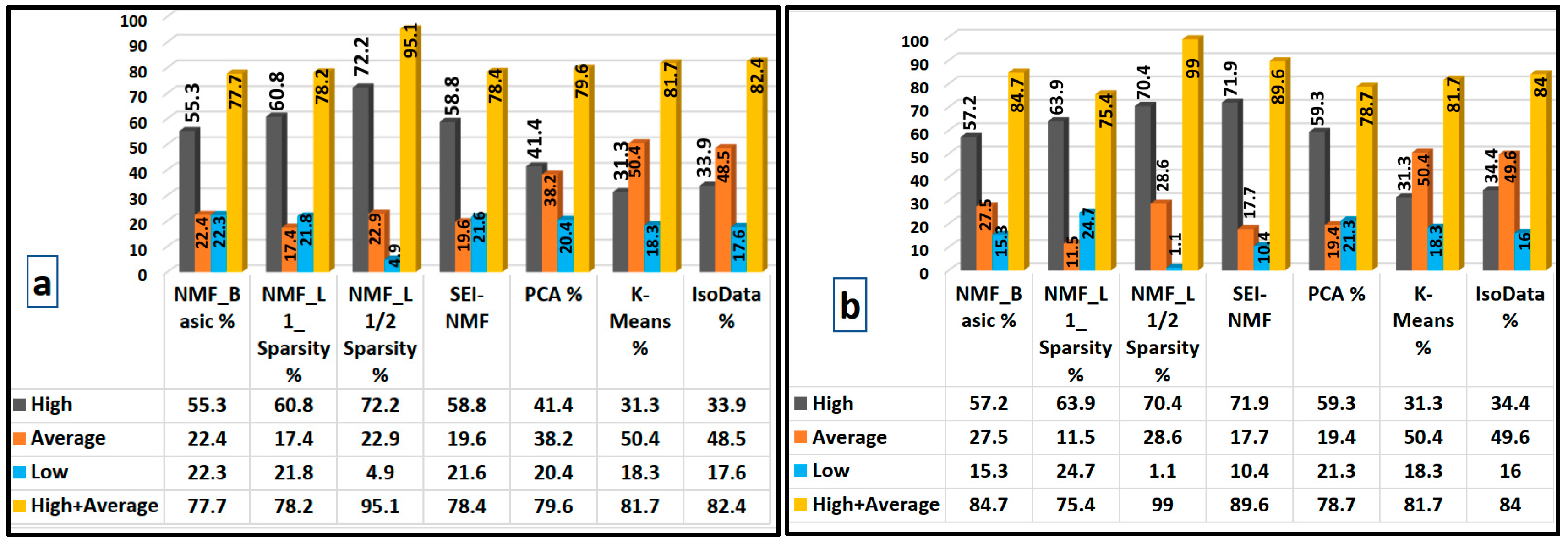
Regarding the first scenario encompassing Sentinel 2, ZGI, and elevation, the results demonstrate that the NMF methods offer superior predictive performance compared to PCA, K-means, and IsoData. Specifically, the L1/2-Sparsity NMF model provided the best results [48] and identified 72.2% of the burned areas as high-risk, with an overall combined classification of 95.1% when high and average risk areas were considered. The L1-Sparsity, Basic NMF, and SEI-NMF models also performed robustly, capturing 60.8%, 55.3%, and 58.8 % as high-risk and 78.2%, 77.7%, and 78.4% as high plus average risk zones, respectively. This consistency across NMF variants suggests a heightened sensitivity to critical fire-prone features, which may be attributed to NMF’s decomposition of data into parts-based representations, helping isolate areas with characteristics strongly associated with fire susceptibility [38,48].
In contrast, while yielding 79.6% in the high and average categories, PCA classified only 41.4% of burned areas as high-risk, underscoring its lower precision in identifying zones with the highest fire susceptibility. K-means and IsoData further demonstrated limitations, with high-risk classifications of 31.3% and 33.9%, respectively (Figure 6a), and struggled to identify non-flammable features like water bodies accurately (Figure 5f-5g, and 6f-6g). It can be due to the high sensitivity of K-means and IsoData to outliers, high dimensionality, and noise [35].
On the other hand, when only Sentinel-2 bands and the ZGI index were included, the results show that the SEI-NMF method outperformed all other models in predicting fire-prone areas, capturing approximately 72% of burned areas as high-risk and nearly 90% as high and average risk combined. The L1/2-Sparsity NMF model followed closely, identifying 70.4% as high-risk and 99% as high-plus-average areas. Basic NMF and L1-Sparsity models achieved around 57% and 64% in high-risk classifications, respectively (Figure 7b). When DEM data is included, its inherent characteristics may introduce noise, which can disrupt accurate spectral discrimination compared to using Sentinel data alone, which has distinct and consistent spectral properties. DEM data may dilute spectral signals by emphasizing elevation-driven features that are less relevant to the land cover targets (endmembers), reducing the algorithm’s capacity to focus on the critical spectral characteristics of endmembers. By relying solely on Sentinel-2 data, the modified NMF can better isolate and analyze the pure spectral signals, free from the noise introduced by mixed-data characteristics of DEM. This characteristic can also be generalized to other data like slope, aspect, and distance from roads, which have been widely used to detect fire-prone areas, especially supervised methods.
PCA and K-means results remained largely unchanged from previous analyses (where elevation was included), with K-means and PCA showing limited ability to differentiate high-risk areas. Additionally, the NMF models showed a solid ability to recognize non-fire-prone regions such as water bodies, mountainous areas with minimal vegetation cover, and urban zones, which typically exhibit the lowest susceptibility to wildfires (yellow polygons in Figure 4a- 4d and 5a-5c). These regions were consistently classified as low-risk areas, highlighting NMF’s effectiveness in distinguishing between fire-prone and non-fire-prone landscapes. PCA similarly identified these low-susceptibility areas accurately, although with slightly less precision than the NMF models (Figure 4e and 5e). This ability to detect and categorize non-flammable zones with high accuracy further validates the NMF methods’ applicability in comprehensive fire-risk mapping, ensuring non-vulnerable areas are correctly excluded from high-risk classifications. K-means and IsoData failed to detect water bodies or urban areas as low fire-prone areas. If the K-means and IsoData methods are adjusted such that water bodies are classified as low fire-prone areas, it could lead to inconsistencies with ground observations and the performance of other methods. Typically, water bodies, due to their lack of vegetation and low flammability, are expected to be classified as low-risk areas for wildfires. However, when not correctly distinguishing water bodies, these methods may misclassify them. This would conflict with observations and other models’ classifications, which align water bodies with areas of minimal fire susceptibility. Adjusting the classification could disrupt the model’s consistency, as real-world fire-prone zones (such as areas with dense vegetation) would be misrepresented, undermining the overall validity of the classification. This could lead to a less accurate representation of fire-prone areas and affect resource allocation and fire management strategies based on these classifications.
The urban area, such as Marivan town (shown as a black polygon inside the maps), is also recognized as low fire-prone. The performance of the methods used within the two scenarios differed, with and without elevation data. When elevation was considered, almost all methods failed to detect it as a low fire-prone area, while excluding elevation, practically all NMF methods and PCA recognized it accurately, and even K-means and IsoData partly recognized it. However, the NMF-L1/2 method recognizes the town as partly average and low fire-prone. The results also showed that 150 iterations were generally enough to achieve stable NMF outcomes (Figure 4a-4d). However, testing different iteration sizes or using predefined, reliable initial values could further improve model performance.
NMF has shown great promise in various fields, particularly in dimensionality reduction and uncovering hidden patterns within complex data. Despite its proven capabilities, NMF has not yet been applied in the context of wildfire detection and burn severity mapping [41,48]. This gap presents a significant opportunity, as NMF’s ability to handle heterogeneous data could enhance wildfire research, especially when dealing with the varied and complex features found in wildfire datasets. Some methods, like Segmented Non-negative Matrix Factorization (SNMF), have outperformed PCA and NMF in hyperspectral image analysis [64], indicating a significant advantage in data processing. Yet, the potential of NMF in wildfire applications remains untapped despite its successes in other fields [64,67].
In contrast, other techniques like PCA have been utilized in this domain. Zheng et al. [68] demonstrated the effectiveness of PCA with Polarimetric Synthetic Aperture Radar (PolSAR) data and random forest algorithm, achieving promising correlations by integrating vegetation structure. Similarly, PCA has been used in multiple studies, such as those by Henry and Epting et al., to differentiate burned areas using Landsat data [69,70].
Additionally, hybrid methods like K-means clustering combined with neural networks and the Forest Fire Hybrid Detection Model (FFHDM) have demonstrated remarkable success in fire detection. These techniques utilize clustering and advanced classifiers to improve detection efficiency [71,72].
By integrating NMF into wildfire research, especially with other advanced techniques like PCA and machine learning models, researchers could unlock new potential for more accurate and efficient wildfire detection and burn severity mapping. While advanced deep learning methods could potentially improve performance, they often require large labeled datasets and significant computational resources, which may not be feasible in time-sensitive post-fire scenarios. Our choice of interpretable, lightweight methods such as NMF and K-means enables more practical deployment in operational wildfire monitoring. Future work may investigate hybrid approaches combining deep feature extraction with unsupervised clustering.
5. Conclusions
This study underscores the critical need for effective fire susceptibility mapping in SM and SA regions, which face increasing wildfire threats. By proposing a modified NMF method and comparing it with other unsupervised techniques such as PCA, K-means, and IsoData, the research provides valuable insights into the potential of satellite-derived data for wildfire risk prediction. The results demonstrate that NMF, especially the L1/2 sparsity method, performs best in detecting high-risk fire areas when using Sentinel-2 bands, ZGI, and elevation data, achieving up to 72% high-risk areas. When elevation data was not considered, the proposed NMF method performed similarly well, identifying 72% of burned areas as high-risk and nearly 90% as high and average combined.
However, challenges remain in improving the accuracy of these unsupervised models. Variability in results due to random initialization and the non-convex nature of these algorithms suggests the need for more controlled experimentation. To address these challenges, future research could explore integrating NMF results into supervised machine learning models, where they could serve as features to enhance classification accuracy. Additionally, using predefined initial values and testing different iteration sizes may improve model stability and reduce outcome variability.
Further improvements could include refining the classification of non-fire-prone areas, such as water bodies and urban zones, which K-means and IsoData struggled to classify correctly. A more robust approach would involve integrating these unsupervised methods with supervised classification techniques, where ground truth data or expert labels could provide the final validation layer. By doing so, building more reliable and contextually accurate fire risk maps would be possible. Moreover, combining these satellite-based models with environmental factors like weather patterns, human activities, and land cover changes could offer a more holistic view of fire susceptibility.
In conclusion, this study provides a valuable foundation for future wildfire management strategies in SM and SA regions. This framework is potentially applicable on other areas with similar weather regimes, such as Portugal, Spain, and Greece. Future work should focus on improving the consistency of unsupervised methods and exploring their integration into supervised machine learning methods, which could result in more accurate, reliable, and actionable fire-prone area predictions.
Author Contributions
Conceptualization, I.R. and W.B; methodology, I.R and W.B.; software, I.R. and W.B; investigation, I.R., W.B, and L.D.; data curation, I.R.; writing—original draft preparation, I.R. and W.B; writing—review and editing, I.R., L.D., and A.C.T.; funding acquisition, A.C.T. and L.D. All authors have read and agreed to the published version of the manuscript.
Funding
This research received no external funding
Institutional Review Board Statement
Not applicable.
Informed Consent Statement
Not applicable.
Acknowledgments
This work is supported by national funding awarded by FCT—Foundation for Science and Technology, I.P., projects UIDB/04683/2020 (https://doi.org/10.54499/UIDB/04683/2020), UIDP/04683/2020 (https://doi.org/10.54499/UIDP/04683/2020) and UID/04683-INSTITUTO DE CIÊNCIAS DA TERRA.
Conflicts of Interest
The authors declare no conflict of interest.
References
- D.A.; Nunes, J.P.; Lucas-Borja, M.E. Improvement of Seasonal Runoff and Soil Loss Predictions by the MMF (Morgan-Morgan-Finney) Model after Wildfire and Soil Treatment in Mediterranean Forest Ecosystems. Catena 2020, 188, 104415. [CrossRef]
- Bowman, D.M.J.S.; Moreira-Muñoz, A.; Kolden, C.A.; Chavez, R.O.; Munoz, A.A.; Salinas, F.; Gonzalez-Reyes, A.; Rocco, R.; de la Barrera, F.; Williamson, G.J.; et al. Human-environmental drivers and impacts of the globally extreme 2017 Chilean fires. Ambio 2019, 48, 350–362. [Google Scholar] [CrossRef] [PubMed]
- Geist, H.J.; Lambin, E.F. Proximate Causes and Underlying Driving Forces of Tropical Deforestation. BioScience 2002, 52, 143–150. [Google Scholar] [CrossRef]
- Suryabhagavan, K.V.; Alemu, M.; Balakrishnan, M. GIS-Based Multi-Criteria Decision Analysis for Forest Fire Susceptibility Mapping: A Case Study in Harenna Forest, Southwestern Ethiopia. Trop. Ecol. 2016, 57, 33–43. [Google Scholar]
- Dos Reis, M.; Graça, P.M.L. de A.; Yanai, A.M.; Ramos, C.J.P.; Fearnside, P.M. Forest Fires and Deforestation in the Central Amazon: Effects of Landscape and Climate on Spatial and Temporal Dynamics. J. Environ. Manag. 2021, 288, 112310. [CrossRef]
- Keenan, R.J. Climate Change Impacts and Adaptation in Forest Management: A Review. Ann. For. Sci. 2015, 72, 145–167. [Google Scholar] [CrossRef]
- Simioni, G.; Marie, G.; Davi, H.; Martin-St Paul, N.; Huc, R. Natural Forest Dynamics Have More Influence than Climate Change on the Net Ecosystem Production of a Mixed Mediterranean Forest. Ecol. Model. 2020, 416, 108921. [Google Scholar] [CrossRef]
- Rahimi, I.; Duarte, L.; Teodoro, A.C. Zagros Grass Index—A New Vegetation Index to Enhance Fire Fuel Mapping: A Case Study in the Zagros Mountains. Sustainability 2024, 16, 3900. [Google Scholar] [CrossRef]
- Kala, C.P. Environmental and socioeconomic impacts of forest fires: A call for multilateral cooperation and management interventions. Nat. Hazards Res. 2023, 3, 286–294. [Google Scholar] [CrossRef]
- Teodoro, A.C.; Duarte, L. Forest fire risk maps: A GIS open source application—A case study in Norwest of Portugal. Int. J.Geogr. Inf. Sci. 2013, 27, 699–720. [Google Scholar] [CrossRef]
- Ghorbanzadeh, O.; Valizadeh, K.K.; Blaschke, T.; Aryal, J.; Naboureh, A.; Einali, J.; Bian, J. Spatial Prediction of Wildfire Susceptibility Using Field Survey GPS Data and Machine Learning Approaches. Fire 2019, 2(3), 43. [Google Scholar] [CrossRef]
- Gong, J.; Jin, T.; Cao, E.; Wang, S.; Yan, L. Is Ecological Vulnerability Assessment Based on the VSD Model and AHP-Entropy Method Useful for Loessial Forest Landscape Protection and Adaptive Management? A Case Study of Ziwuling Mountain Region, China. Ecol. Indic. 2022, 143, 109379. [Google Scholar] [CrossRef]
- Lamat, R.; Kumar, M.; Kundu, A.; Lal, D. Forest Fire Risk Mapping Using Analytical Hierarchy Process (AHP) and Earth Observation Datasets: A Case Study in the Mountainous Terrain of Northeast India. SN Appl. Sci. 2021, 3. [Google Scholar] [CrossRef]
- Arca, D.; Hacısalihoğlu, M.; Kutoğlu, Ş.H. Producing Forest Fire Susceptibility Map via Multi-Criteria Decision Analysis and Frequency Ratio Methods. Nat. Hazards 2020, 104(1), 73–89. [Google Scholar] [CrossRef]
- Tiwari, A.; Shoab, M.; Dixit, A. GIS-Based FFS Modeling in Pauri Garhwal, India: A Comparative Assessment of Frequency Ratio, Analytic Hierarchy Process, and Fuzzy Modeling Techniques. Nat. Hazards 2021, 105, 1189–1230. [Google Scholar] [CrossRef]
- Moayedi, H.; Mehrabi, M.; Bui, D.T.; Pradhan, B.; Foong, L.K. Fuzzy-Metaheuristic Ensembles for Spatial Assessment of Forest Fire Susceptibility. J. Environ. Manag. 2020, 109867. [Google Scholar] [CrossRef] [PubMed]
- Shi, C.; Zhang, F. A forest fire susceptibility modeling approach based on integration of machine learning algorithms. Forests 2023, 14, 1506. [Google Scholar] [CrossRef]
- Trucchia, A.; Meschi, G.; Fiorucci, P.; Gollini, A.; Negro, D. Defining wildfire susceptibility maps in Italy for understanding seasonal wildfire regimes at the national level. Fire 2022, 5, 30. [Google Scholar] [CrossRef]
- Saha, S.; Bera, B.; Shit, P.K.; Bhattacharjee, S.; Sengupta, N. Prediction of forest fire susceptibility applying machine and deep learning algorithms for conservation priorities of forest resources. Remote Sensing Applications: Society and Environment 2023, 29, 100917. [Google Scholar] [CrossRef]
- Piao, Y.; Lee, D.; Park, S.; Kim, H.G.; Jin, Y. Forest fire susceptibility assessment using Google Earth Engine in Gangwon-do, Republic of Korea. Geomatics, Natural Hazards and Risk 2022, 13(1), 432–450. [CrossRef]
- Kalantar, B.; Ueda, N.; Idrees, M.O.; Janizadeh, S.; Ahmadi, K.; Shabani, F. Forest fire susceptibility prediction based on machine learning models with resampling algorithms on remote sensing data. Remote Sensing 2020, 12, 3682. [Google Scholar] [CrossRef]
- Mishra, M.; Guria, R.; Baraj, B.; Nanda, A.P.; Santos, C.A.G.; Da Silva, R.M.; Laksono, F.A.T. Spatial analysis and machine learning prediction of forest fire susceptibility: A comprehensive approach for effective management and mitigation. Science of the Total Environment 2024, 926, 171713. [Google Scholar] [CrossRef]
- Sharma, L.K.; Gupta, R.; Naureen Fatima, N. Assessing the predictive efficacy of six machine learning algorithms for the susceptibility of Indian forests to fire. International Journal of Wildland Fire 2022, 31(8), 735–758. [Google Scholar] [CrossRef]
- Maffei, C.; Menenti, M. An application of the perpendicular moisture index for the prediction of fire hazard. EARSeleProceedings 2014, 13. [Google Scholar]
- Sulova, A.; Arsanjani, J.J. Exploratory Analysis of Driving Force of Wildfires in Australia: An Application of Machine Learning within Google Earth Engine. Remote Sens. 2020, 13(1), 10. [Google Scholar] [CrossRef]
- Sivrikaya, F.; Küçük, Ö. Modeling forest fire risk based on GIS-based analytical hierarchy process and statistical analysis in the Mediterranean region. Ecological Informatics 2021, 68, 101537. [Google Scholar] [CrossRef]
- Chaleplis, K.; Walters, A.; Fang, B.; Lakshmi, V.; Gemitzi, A. A Soil Moisture and Vegetation-Based Susceptibility Mapping approach to wildfire events in Greece. Remote Sens. 2024, 16(10), 1816. [Google Scholar] [CrossRef]
- Chuvieco, E.; Cocero, D.; Riaño, D.; Martin, P.; Martínez-Vega, J.; De La Riva, J.; Pérez, F. Combining NDVI and surface temperature for the estimation of live fuel moisture content in forest fire danger rating. Remote Sens. Environ. 2004, 92(3), 322–331. [Google Scholar] [CrossRef]
- Luz, A.E.O.; Negri, R.G.; Massi, K.G.; Colnago, M.; Silva, E.A.; Casaca, W. Mapping fire susceptibility in the Brazilian Amazon forests using multitemporal remote sensing and time-varying unsupervised anomaly detection. Remote Sensing. 2022, 14, 2429. [Google Scholar] [CrossRef]
- Yankovich, K.S.; Yankovich, E.P.; Baranovskiy, N.V. Classification of vegetation to estimate forest fire danger using LANDSAT 8 Images: Case study. Math. Probl. Eng. 2019, 6296417. [Google Scholar] [CrossRef]
- Zaidi, A. Predicting wildfires in Algerian forests using machine learning models. Heliyon 2023, 9(7), e18064. [Google Scholar] [CrossRef]
- Wang, M.; Gao, G.; Huang, H.; Heidari, A.A.; Zhang, Q.; Chen, H.; Tang, W. A principal component Analysis-Boosted dynamic Gaussian mixture clustering model for ignition factors of Brazil’s rainforests. IEEE Access 2021, 9, 145748–145762. [Google Scholar] [CrossRef]
- Jolliffe, I.T. Principal Component Analysis; Springer: New York, NY, USA, 2002. [Google Scholar]
- Jarocińska, A.; Kopeć, D.; Kycko, M. Comparison of Dimensionality Reduction Methods on Hyperspectral Images for the Identification of Heathlands and Mires. Sci. Rep. 2024, 14(1). [CrossRef]
- Ma, Z.; Liu, Z.; Zhao, Y.; Zhang, L.; Liu, D.; Ren, T.; Zhang, X.; Li, S. An Unsupervised Crop Classification Method Based on Principal Components Isometric Binning. ISPRS Int. J. Geo-Inf. 2020, 9, 648. [Google Scholar] [CrossRef]
- Lv, Z.; Liu, T.; Shi, C.; Benediktsson, J.A.; Du, H. Novel Land Cover Change Detection Method Based on K-Means Clustering and Adaptive Majority Voting Using Bitemporal Remote Sensing Images. IEEE Access 2019, 7, 34425–34437. [Google Scholar] [CrossRef]
- Lillesand, T.; Kiefer, R. Remote Sensing and Image Interpretation, 4th ed.; Wiley: New York, NY, USA, 2000. [Google Scholar]
- Bioucas-Dias, J.M.; Plaza, A.; Dobigeon, N.; Parente, M.; Du, Q.; Gader, P.; Chanussot, J. Hyperspectral Unmixing Overview: Geometrical, Statistical, and Sparse Regression-Based Approaches. IEEE J. Sel. Top. Appl. Earth Obs. Remote Sens. 2012, 5(2), 354–379. [Google Scholar] [CrossRef]
- Thein, A.M.; Htwe, A.N. Based on Principal Component Analysis of Land Use Land Cover Change Detection Using Landsat Satellite Images (Case Study Mandalay City). Proceedings of the 2023 IEEE Conference on Computer Applications (ICCA), Yangon, Myanmar, 2023, pp. 147–152. [CrossRef]
- Lv, Z.; Liu, T.; Shi, C.; Benediktsson, J.A.; Du, H. Novel Land Cover Change Detection Method Based on k-Means Clustering and Adaptive Majority Voting Using Bitemporal Remote Sensing Images. IEEE Access 2019, 7, 34425–34437. [Google Scholar] [CrossRef]
- Huang, R.; Jiao, H.; Li, X.; Chen, S.; Xia, C. Hyperspectral unmixing using robust deep nonnegative matrix factorization. Remote Sens. 2023, 15(11), 2900. [Google Scholar] [CrossRef]
- Berry, M.W.; Browne, M.; Langville, A.N.; Pauca, V.P.; Plemmons, R.J. Algorithms and Applications for Approximate Nonnegative Matrix Factorization. Comput. Stat. Data Anal. 2007, 52, 155–173. [Google Scholar] [CrossRef]
- Jazirehi, M.H.; Rostaaghi, E.M. Silviculture in Zagros; University of Tehran Press: Tehran, Iran, 2003; 560p. Available online: https://www.scirp.org/reference/referencespapers?referenceid=1852053 (accessed on 20 November 2023).
- El-Moslimany, A.P. Ecology and Late-Quaternary History of the Kurdo-Zagrosian Oak Forest Near Lake Zeribar, Western Iran. Vegetation 1986, 68, 55–63. [Google Scholar] [CrossRef]
- Pourhashemi, M.; Zandebasiri, P.; Panahi, S. Structural Characteristics of Oak Coppice Stands of Marivan Forests. Iran. J. Plant Res. 2014, 27, 766–776. [Google Scholar]
- European Space Agency (ESA). Copernicus Open Access Hub, Sentinel-2 Level-2A Products. Available online: https://scihub.copernicus.eu.
- USGS EROS Archive. Digital Elevation - Shuttle Radar Topography Mission (SRTM). Available online: https://www.usgs.gov/centers/eros/science/usgs-eros-archive-digital-elevation-shuttle-radar-topography-mission-srtm-1.
- Qian, Y.; Jia, S.; Zhou, J.; Robles-Kelly, A. Hyperspectral unmixing via L1/2 sparsity-constrained nonnegative matrix factorization. IEEE Trans. Geosci. Remote Sens. 2011, 49(11), 4282–4297. [Google Scholar] [CrossRef]
- Huang, Q.; Yin, X.; Chen, S.; Wang, Y.; Chen, B. Robust Nonnegative Matrix Factorization with Structure Regularization. Neurocomputing 2020, 412, 72–90. [Google Scholar] [CrossRef]
- National Cartographic Center of Iran (NCC), https://en.ncc.gov.ir/Services.
- Lee, D.D.; Seung, H.S. Learning the parts of objects by non-negative matrix factorization. Nature 1999, 401(6755), 788. [Google Scholar] [CrossRef]
- Wu, W.; Jia, Y.; Kwong, S.; Hou, J. Pairwise constraint propagation-induced symmetric nonnegative matrix factorization. IEEE Trans. Neural Netw. Learn. Syst. 2018, 29(12), 6348–6361. [Google Scholar] [CrossRef] [PubMed]
- Faraji, M.; Seyedi, S.A.; Akhlaghian Tab, F.; Mahmoodi, R. Multi-label feature selection with global and local label correlation. Expert Syst. With Appl. 2024, 246, 123198. [Google Scholar] [CrossRef]
- Li, H.; Li, K.; An, J.; Zhang, W.; Li, K. An efficient manifold regularized sparse non-negative matrix factorization model for large-scale recommender systems on GPUs. Inf. Sci. 2019. [CrossRef]
- Liu, X.; Wang, W.; He, D.; Jiao, P.; Jin, D.; Cannistraci, C.V. Semi-supervised community detection based on non-negative matrix factorization with node popularity. Inf. Sci. 2017, 381, 304–321. [Google Scholar] [CrossRef]
- Seyedi, S.A.; Tab, F.A.; Lotfi, A.; Salahian, N.; Chavoshinejad, J. Elastic adversarial deep nonnegative matrix factorization for matrix completion. Inf. Sci. 2023, 621, 562–579. [Google Scholar] [CrossRef]
- Lee, D.D.; Seung, H.S. Algorithms for non-negative matrix factorization. In Advances in Neural Information Processing Systems, 2001; pp. 556–562.
- Lu, X.; Wu, H.; Yuan, Y.; Yan, P.; Li, X. Manifold regularized sparse NMF for hyperspectral unmixing. IEEE Trans. Geosci. Remote Sens. 2013, 51(5), 2815–2826. [Google Scholar] [CrossRef]
- Xu, R.; Wunsch, D. Survey of clustering algorithms. IEEE Trans. Neural Netw. *2005, *16, 645–678. [CrossRef]
- Kang, J.; Wang, Z.; Sui, L.; Yang, X.; Ma, Y.; Wang, J. Consistency Analysis of Remote Sensing Land Cover Products in the Tropical Rainforest Climate Region: A Case Study of Indonesia. Remote Sens. 2020, 12, 1410. [Google Scholar] [CrossRef]
- Wei, R.; Ye, C.; Sui, T.; Ge, Y.; Li, Y.; Li, J. Combining Spatial Response Features and Machine Learning Classifiers for Landslide Susceptibility Mapping. Int. J. Appl. Earth Obs. Geoinf. 2022, 107, 102681. [Google Scholar] [CrossRef]
- Meyer, H.; Pebesma, E. Machine Learning-Based Global Maps of Ecological Variables and the Challenge of Assessing Them. Nat. Commun. 2022, 13, 29838. [Google Scholar] [CrossRef]
- Giddey, B.L.; Baard, J.A.; Kraaij, T. Verification of the differenced Normalised Burn Ratio (dNBR) as an index of fire severity in Afrotemperate Forest. South Afr. J. Bot. 2021, 146, 348–353. [Google Scholar] [CrossRef]
- Sivrikaya, F.; Günlü, A.; Küçük, Ö.; Ürker, O. Forest fire risk mapping with Landsat 8 OLI images: Evaluation of the potential use of vegetation indices. Ecol. Informatics 2024, 79, 102461. [Google Scholar] [CrossRef]
- Guo, Z.; Min, A.; Yang, B.; Chen, J.; Li, H. A Modified Huber Nonnegative Matrix Factorization Algorithm for Hyperspectral Unmixing. IEEE J. Sel. Top. Appl. Earth Obs. Remote Sens. 2021, 14, 5559–5571. [Google Scholar] [CrossRef]
- Bari, M.H.; Ahmed, T.; Afjal, M.I.; Nitu, A.M.; Uddin, M.P.; Marjan, M.A. Segmented Nonnegative Matrix Factorization for Hyperspectral Image Classification. In Proceedings of the International Conference on Electrical, Computer and Communication Engineering (ECCE), Chittagong, Bangladesh; 2023; pp. 1–5. [Google Scholar] [CrossRef]
- Zhao, L.; Zhuang, G.; Xu, X. Facial expression recognition based on PCA and NMF. In Proceedings of the 7th World Congress on Intelligent Control and Automation (WCICA), Chongqing, China; 2008; pp. 6826–6829. [Google Scholar] [CrossRef]
- Zheng, Z.; Zeng, Y.; Zou, B.; Xie, Q.; Xian, W.; Xu, W.; Liu, Y.; Liu, Z. Assessing the burn severity of wildfires by incorporating vegetation structure information. Geomatics Nat. Hazards Risk *2024, *15, 1. [CrossRef]
- Henry, M.C. Comparison of single- and multi-date Landsat data for mapping wildfire scars in Ocala National Forest, Florida. Photogramm. Eng. Remote Sens. *2008, *74, 881–891. [CrossRef]
- Epting, J.; Verbyla, D.; Sorbel, B. Evaluation of remotely sensed indices for assessing burn severity in interior Alaska using Landsat TM and ETM+. Remote Sens. Environ. *2005, *96, 328–339. [CrossRef]
- Oladimeji, M.O.; Ghavami, M.; Dudley, S. A new approach for event detection using k-means clustering and neural networks. In Proceedings of the International Joint Conference on Neural Networks (IJCNN); 2015. [Google Scholar] [CrossRef]
- Lakshmanaswamy, P.; Sundaram, A.; Sudanthiran, T. Prioritizing the right to environment: enhancing forest fire detection and prevention through satellite data and machine learning algorithms for early warning systems. Remote Sens. Earth Syst. Sci. *2024*. [CrossRef]
Figure 1.
Location of the study Area. Marivan, Sarvabad in western Iran.
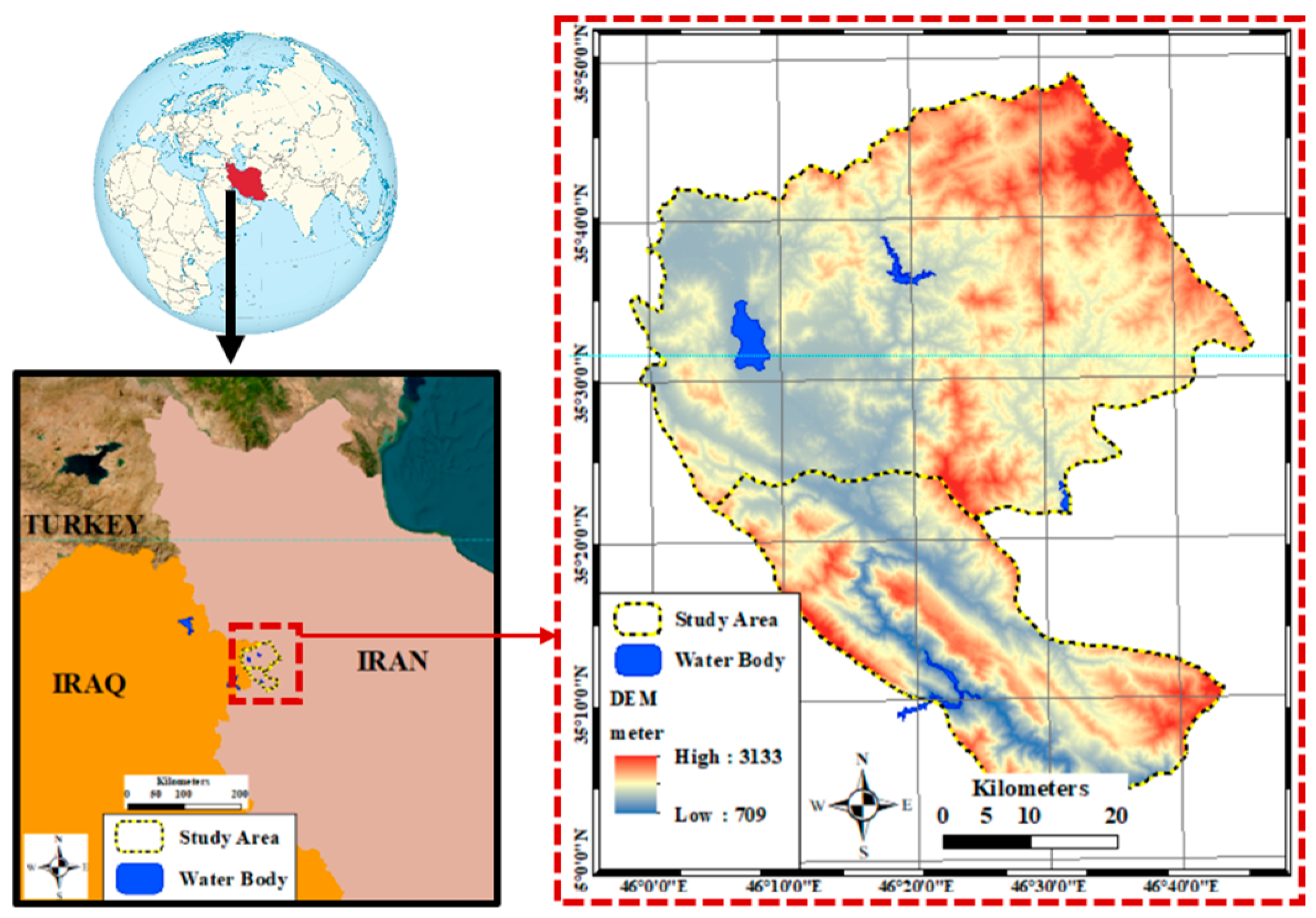
Figure 2.
SEI-NMF Methodological Framework. The red-border steps show the proposed modifications.
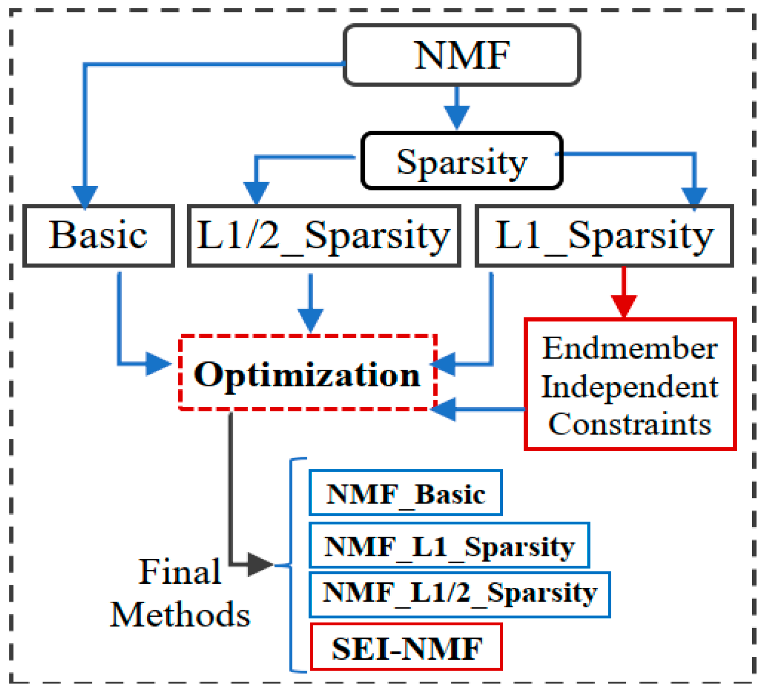
Figure 3.
Methodological Framework.
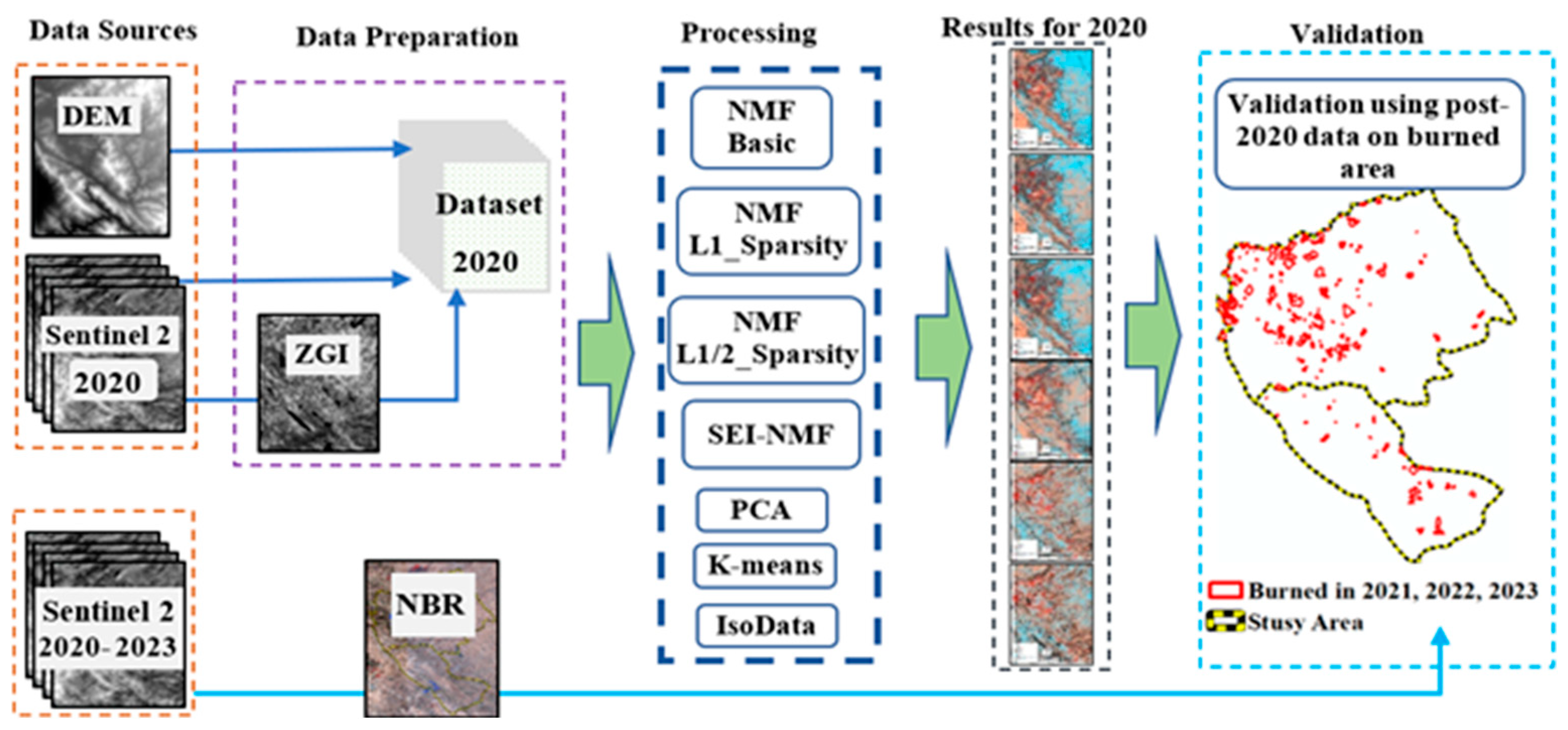
Figure 4.
The convergence rate of each NMF method per iteration.
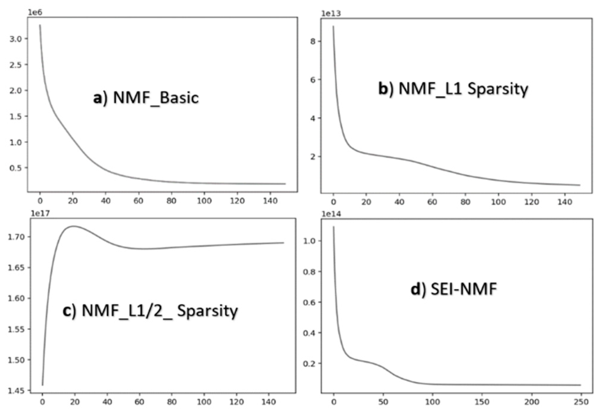
Figure 5.
Maps generated by a) Basic NMF, b) L1-Sparsity, c) L1/2-Sparsity, d) SEI-NMF, e) PCA, f) K-means, g) IsoData using Sentinel 2 bands, ZGI, and elevation. The red areas are the burned areas from 2021 to 2023. The yellow polygons represent the area with water bodies, and the black polygon represents Marivan town.
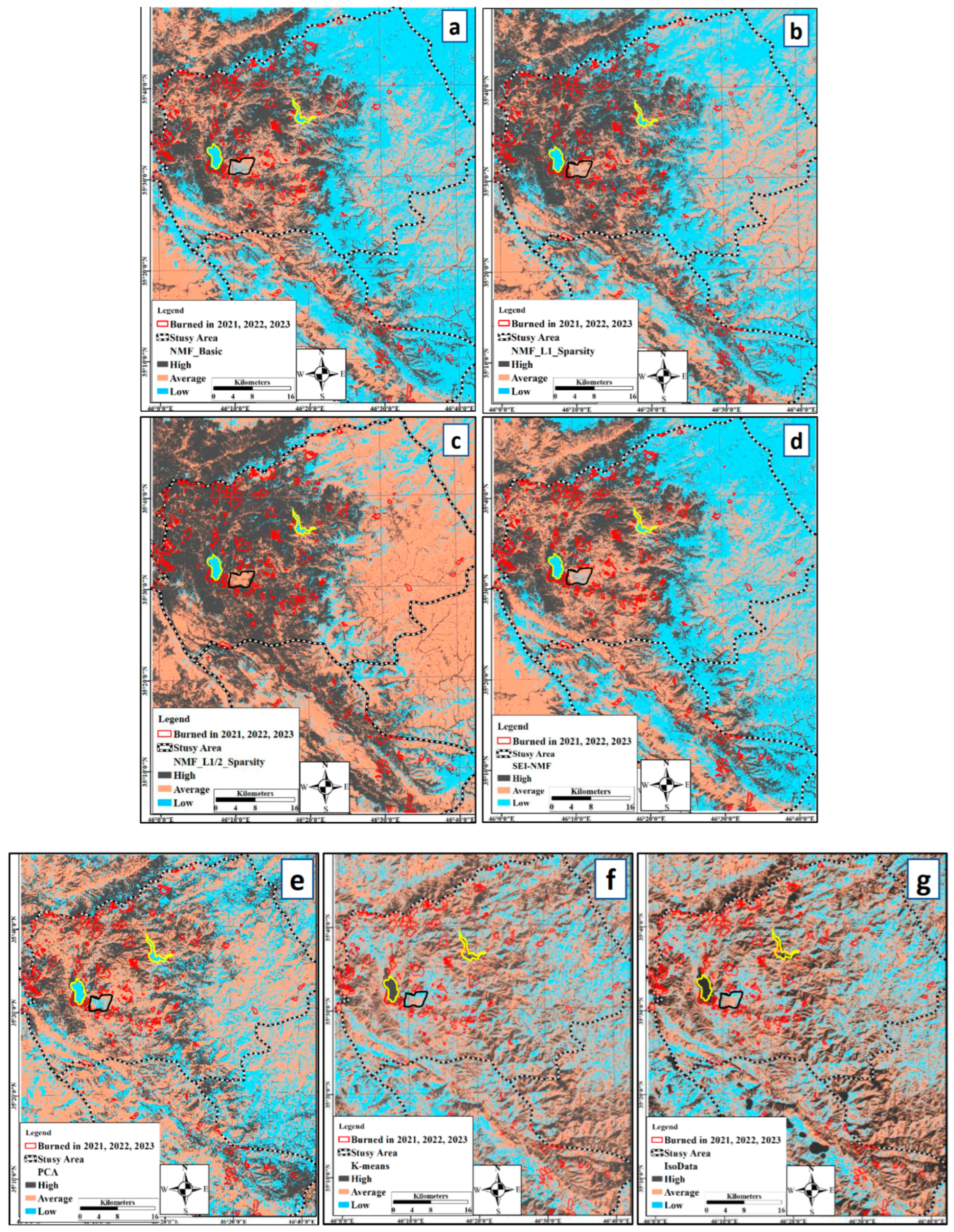
Figure 6.
Maps generated by a) Basic NMF, b) L1-Sparsity, c) L1/2-Sparsity, d) SEI-NMF, e) PCA, f) K-means, g) IsoData using Sentinel 2 bands, and ZGI. The red areas are the burned areas from 2021 to 2023. The yellow polygons represent the area with water bodies, and the black polygon represents Marivan town.
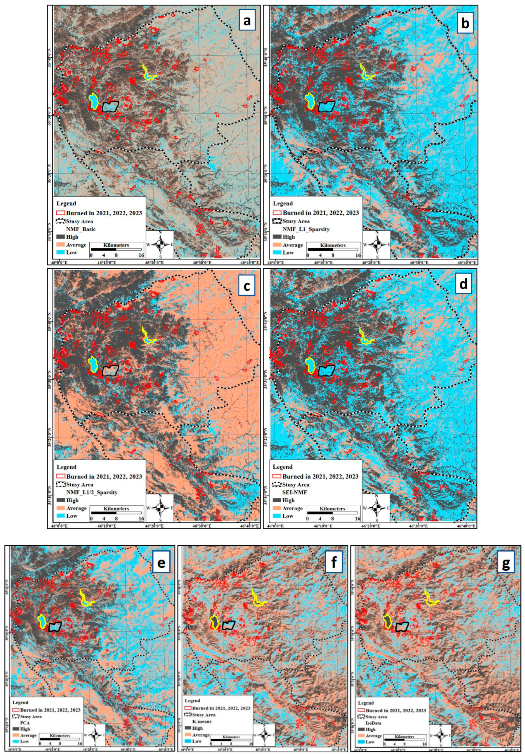
Figure 7.
Statistical distribution of each class for 2020 within the post-2020 burned area, regarding a) Sentinel 2 data, ZGI, and the elevation, and b) only Sentinel 2 bands and ZGI.
Figure 7.
Statistical distribution of each class for 2020 within the post-2020 burned area, regarding a) Sentinel 2 data, ZGI, and the elevation, and b) only Sentinel 2 bands and ZGI.

Disclaimer/Publisher’s Note: The statements, opinions and data contained in all publications are solely those of the individual author(s) and contributor(s) and not of MDPI and/or the editor(s). MDPI and/or the editor(s) disclaim responsibility for any injury to people or property resulting from any ideas, methods, instructions or products referred to in the content. |
© 2025 by the authors. Licensee MDPI, Basel, Switzerland. This article is an open access article distributed under the terms and conditions of the Creative Commons Attribution (CC BY) license (http://creativecommons.org/licenses/by/4.0/).
Copyright: This open access article is published under a Creative Commons CC BY 4.0 license, which permit the free download, distribution, and reuse, provided that the author and preprint are cited in any reuse.


