Submitted:
12 April 2025
Posted:
15 April 2025
You are already at the latest version
Abstract
With ever increasing renewable energy sources, such as wind and solar, being interconnected to power systems, the grid strength, as measured by existing short-circuit ratio (SCR) measures, will become weaker. The high penetration of renewable generation has posed new challenges to the stability of power grids, and grid-forming (GFM) inverters have been introduced as an effective solution to improve power system stability under these conditions. However, the impact of grid strength (e.g., SCR and X/R ratio) on the stability of GFM and legacy grid-following (GFL) inverters is still not well studied, especially because no hardware test/evaluation work has been carried out. To fill this gap, this paper conducts a comprehensive hardware test of two commercial inverters (which can operate in either GFM or GFL control) under varying grid strengths (SCR and X/R) to gain a comprehensive understanding of how grid strength can impact the stability of GFM and GFL inverters. This comprehensive evaluation using commercial inverters reveals that both X/R and SCR affect the voltage stability of GFM and GFL inverters, but they exhibit different trends under varying grid impedances. X/R affects the voltage stability more than SCR; reducing X/R has a negative impact on the GFM inverter’s stability, but it has a positive impact on the GFL’s stability (this indicates that the GFM inverter might have better stability with transmission systems with a higher X/R ratio, and GFL inverters might have better stability with distribution systems with a lower X/R ratio); and under the same X/R with varying SCRs, the GFM inverter’s point of interconnection (POI) voltage decreases with a lower SCR, whereas the GFL inverter’s POI voltage increases with a lower SCR.
Keywords:
GFM inverters
; GFL inverters
; SCR
; X/R ration
; Grid
; renewable energy
1. Introduction
The rapid increase in the interconnection of inverter-based resources (IBRs), such as wind and solar power, is reducing system inertia and strength, thereby affecting the frequency and voltage stability of the power grid, making it crucial to analyze power system stability driven by IBRs [1]. The stability analysis becomes increasingly complicated with high penetrations of IBRs because it requires careful considerations of various factors, including the grid operating conditions, grid strength, controls and control parameters of IBRs, as well as
This work was authored by the National Renewable Energy Laboratory, operated by Alliance for Sustainable Energy, LLC, for the U.S. Department of Energy (DOE) under Contract No. DE-AC36-08GO28308. Funding provided by the U.S Department of Energy Office of Energy Efficiency and Renewable Energy Solar Energy Technologies Office Agreement Number 38637. The views expressed in the article do not necessarily represent the views of the DOE or the U.S. Government. The U.S. Government retains and the publisher, by accepting the article for publication, acknowledges that the U.S. Government retains a nonexclusive, paid-up, irrevocable, worldwide license to publish or reproduce the published form of this work, or allow others to do so, for U.S. Government purposes.
The X/R ratio of the feeder [2]. In particular, many research efforts have focused on studying how grid strength and the grid impedance X/R ratio impact grid-forming (GFM) and grid- following (GFL) inverters. The research in [2] shows that the stability of both GFL and GFM inverters will deteriorate when increasing the X/R ratio; the X/R ratio has a great impact on the GFL inverter under a weaker power grid, whereas the X/R ratio has a greater impact on the GFM inverter under a strong power grid. The effect of the X/R ratio on reactive power control and voltage stability in distribution systems with wind plants is studied in [3]; it shows that lower X/R ratios increase the voltage level, and higher X/R ratios decrease the voltage profile at the PCC, imposing the need for more reactive power support. Reference [4] provides insights on how different X/R ratios affect the GFL inverters’ controls: When the X/R is in a higher range, the interaction is between the grid impedance and the phase-locked-loop (PLL), and when the X/R is in a lower range, the interaction is among the grid impedance, PLL, and current loop.
The study of the stability of a GFL inverter under varying
grid strengths shows that the stability of the GFL inverter gradually decreases if the power grid strength decreases, and the adjustment of the control parameters for the current controller and the PLL should be opposite [5]. A complex torque coefficients method is developed to identify the oscil- lation mechanism of a grid-connected doubly fed induction generator wind plant and contributing factors, including the grid strength and the PLL parameters, and a robust controller is developed to damp the oscillations based on the oscillation mode [6]. A novel method of de-terming the system strength across the frequency range is presented to calculate the grid strength impedance metrics, which is useful to determine the enhancement of the GFM inverter in improving the grid voltage stiffness [7]. A small-signal grid strength of a 100% IBR system is developed to identify the grid strength boundary for both GFM and GFL inverters [8], and this methodology can be applied to guide grid planning and operations to address the small-signal stability issues in 100% IBR systems with GFM and GFL inverters. An adaptive inertia control is developed for virtual synchronous machine-based GFM inverters to adjust the virtual inertia with an identified grid impedance to maintain the desired stability margin of the GFM inverter under strong grid conditions [9]. A simple low-order robust controller based on control parameter-plane and D-decomposition is developed in [10] to guarantee the stability of the GFL inverter under varying grid impedances.
All the research works mentioned here are based on numer- ical simulations to study how the grid strength and different X/R ratios impact GFM and GFL inverters from different angles; however, no hardware testing has been done to demon- strate how various grid strengths and X/R ratios impact the hardware GFM and GFL inverters. To address this research gap, this paper conducts hardware tests on the stability of two commercial inverters (which can operate in either GFM or GFL control) under varying grid strengths (SCR and X/R ratio). The grid is emulated by a grid simulator with zero.

Table 1.
Specifications of the two commercial inverters.
| Specification | GFM 1 | GFM 2 |
|---|---|---|
| Capacity (kVA) | 250 | 125 |
| Frequency droop | 0.6% | 0.6% |
| Voltage droop | 5% | 5% |
| Synch check | Yes (GCB and MCB) | Yes |
| ∆ − Y transformer | 500 kVA | 250 kVA |
| Communication protocol | Modbus TCP | Modbus TCP |
B. Testing Scenarios
Based on the definition of SCR (SCR= SP OI= VLL/Z), and physical output impedance, and a physical line emulator with define X/R = m, the corresponding R
SkV A
SkV Achangeable R and X values is connected to the grid simulator and configured to vary the grid impedance. This pure hardware and X values can be
derived as follows:
VLL
setup with two commercial inverters as the devices under test reflects the impact of grid strength and X/R ratio on
R = SCR ∗ SkV A
∗ √1 + m2 (1)
the hardware GFM and GFL inverters. The insightful testing results from the hardware inverters reveal the different voltage stability characteristics of the GFM and GFL inverters, and those observations might be different from analytic studies or simulations because the hardware inverters usually contain features/nonlinearities/protection functions that are either not captured or not captured correctly and completely in those studies.
2. Description of The Hardware Test Setup
A. Testing Objective and Testing Circuit
The testing objective is to evaluate the voltage stability (especially the voltage profile at the point of interconnection (POI)) of the GFM and GFL inverters under varying grid strengths (short-circuit ratio (SCR) and X/R ratio). For the pure hardware experiment test, two commercial inverters are selected as the devices under test. A distribution line emulator with variable impedance is used to emulate the varying grid impedance with different SCRs and X/R ratios. Figure 1 shows the overall laboratory experiment setup. A grid simulator with 270-kVA capacity is used as a grid, and this grid simulator is a stiff voltage source. Its voltage and frequency are internally controlled to output voltage and frequency with nominal values. The line emulator is 480 V and 75 A (62.35 kVA) with maximal R equal to 0.72 Ω and maximal X equal to 0.54 Ω. The relay of the POI switch is configured 70 A to protect the line emulator and any current higher than that will trip off the breaker. For all the tests, the measurement point is located at the Y-side of the transformer that faces the line emulator. The specifications for the two inverters as the devices under test are presented in Table I. Note that each inverter is configured to work in either GFM or GFL control for the test.
X = R ∗ m (2)
SP OI is the short circut power of the POI and SkV A is the rating of the IBR/DER. VLL is the line-line voltage of the POI, and Z is the equivalent grid impedance. We aim to vary the X/R ratio from 6 to 4, 2, 1, 0.5, and 0.25, and under each fixed
X/R ratio, the SCR can vary from 10, to 5, 2.5, and 1.25. The lists of the varying grid impedances for inverters 1 and 2 are presented in Table II and Table III. Because the R and X value of the line emulator have limitations (Rmax = 0.72 and Xmax = 0.54), some scenarios cannot be achieved. The capacity of Inverter 1 is twice that of Inverter 2, and its needed grid impedance is half that of Inverter 2 under the same X/R ratio and SCR. Therefore, it is able to have a larger range of varying grid impedance.
For each inverter, both GFM and GFL control will be tested based on the scenarios defined in the tables. For fair comparison, both GFM and GFL control of each inverter will output the same power. For example, Inverter 1 operating in GFL control mode is dispatched to output 20% active power (due to the limitation of the capacity of the line emulator at 62.3 kVA), and the GFM inverter is also dispatched to output 20% active power. Both commercial inverters are dispatched to output the target active power through dispatching the frequency intercept, f0, when they operate in GFM control in grid-connected mode. This dispatching rule is illustrated in Figure 2. If the GFM inverter’s target power is P ∗, the new frequency intercept is f ′ =f +m P ∗ 60. The reactive power of the GFM inverter is not intentionally controlled.
3. Analytical Studies of Inverters with GFM and GFL Control
The GFL inverter injects active and reactive power into the grid through controlling the injected current, and the GFL inverter behaves as a current source. The GFM inverter injects active and reactive power into the grid through controlling the droop intercept, f ∗ (or phase angle), and V ∗, and the GFM inverter behaves as a voltage source. Even though the GFM and GFL inverter inject the same amount of active and reactive power into the grid, the impact at the POI terminal voltage stability is different. The phasor diagram analysis circuit of the GFM and GFL inverter for power injection is shown in Figure 3.
Table 2.
List of varying grid impedances for Inverter 1.
| X/R | R (Ω) | X (Ω) | SCR |
|---|---|---|---|
| X/R=6 | 0.015 | 0.09 | 10 |
| 0.03 | 0.18 | 5 | |
| 0.06 | 0.36 | 2.5 | |
| X/R=4 | 0.022 | 0.088 | 10 |
| 0.045 | 0.18 | 5 | |
| 0.089 | 0.358 | 2.5 | |
| X/R=2 | 0.041 | 0.082 | 10 |
| 0.082 | 0.16 | 5 | |
| 0.16 | 0.32 | 2.5 | |
| X/R=1 | 0.065 | 0.065 | 10 |
| 0.13 | 0.13 | 5 | |
| 0.26 | 0.35 | 2.5 | |
| X/R=0.5 | 0.0824 | 0.0412 | 10 |
| 0.1649 | 0.0824 | 5 | |
| 0.3297 | 0.1649 | 2.5 | |
| 0.6954 | 0.3297 | 1.25 | |
| X/R=0.25 | 0.0894 | 0.0224 | 10 |
| 0.1788 | 0.0447 | 5 | |
| 0.3576 | 0.0894 | 2.5 | |
| 0.7153 | 0.1788 | 1.25 |
Table 3.
List of varying grid impedances for Inverter 2.
| X/R | R (Ω) | X (Ω) | SCR |
|---|---|---|---|
| X/R=6 | 0.015 | 0.09 | 10 |
| 0.03 | 0.18 | 5 | |
| 0.06 | 0.36 | 2.5 | |
| X/R=4 | 0.022 | 0.088 | 10 |
| 0.045 | 0.18 | 5 | |
| 0.089 | 0.358 | 2.5 | |
| X/R=2 | 0.041 | 0.082 | 10 |
| 0.082 | 0.16 | 5 | |
| 0.16 | 0.32 | 2.5 | |
| X/R=1 | 0.065 | 0.065 | 10 |
| 0.13 | 0.13 | 5 | |
| 0.26 | 0.35 | 2.5 | |
| X/R=0.5 | 0.0824 | 0.0412 | 10 |
| 0.1649 | 0.0824 | 5 | |
| 0.3297 | 0.1649 | 2.5 | |
| 0.6954 | 0.3297 | 1.25 | |
| X/R=0.25 | 0.0894 | 0.0224 | 10 |
| 0.1788 | 0.0447 | 5 | |
| 0.3576 | 0.0894 | 2.5 |
∗
I˙=I + j ∗ I with I = 3 Pand I =- 3 Q. As explained
V ∠θ is the output voltage for the GFM inverter, and I∠θ is the output voltage for the GFL inverter. Rtx and Xtx are the impedances of the transformer. VP OI is the terminal voltage. Rg and Xg are the grid impedance resistive and inductive part, and E∠0 is the grid voltage. In [12], the GFL inverter has indirect voltage control (using reactive power to affect the voltage), and GFM inverter has direct voltage control. This distinction between indirect and direct voltage control causes the GFM and GFL inverters to have different voltage stability characteristics with the same operating points.
4. Experiment Results
To verify the aforementioned analysis for GFM and GFL in- verters operating under varying grid impedances with different combinations of SCR and X/R, a comprehensive laboratory hardware experiment is carried out. Table II and Table III list all the tests that were performed for inverters 1 and 2, respectively. Note that the line emulator has limited R and X values so that the lowest SCR for each X/R is different. For fair comparison, the GFM and GFL inverter are dispatched to output the same active and reactive power. The evaluation results are listed in Figure 4–Figure 7. Each test result is collected with the selected R and X values to meet the specific SCR and X/R, and the results are obtained when the inverter reaches steady state. There is no step change of the grid impedance because the line emulator is not allowed to be changed during the test.
A. Inverter 1 Testing Results
Figure 4 shows the GFM and GFL inverter’s voltage response under varying SCRs with different X/R ratios. The pattern of the voltage stability of both the GFM and GFL inverters can be drawn from those results: (1) For the GFM inverter, with the same X/R ratio, the lower SCR results in the lower voltage. For example, the voltage with SCR=10 has the highest voltage. Whereas for the GFL inverter, with the same X/R ratio, the lower SCR results in the higher voltage. For example, the voltage with SCR=10 has the lowest voltage. This is completely opposite of the GFM inverter. (2) This trend is consistent for all the tests (X/R ratios from 6 to 4, 2, and 1). And there is no inverter tripping in this case. The GFM and GFL inverters maintain good stability, whereas the GFL inverter exhibits overvoltage issues from X/R=2 with SCR=2.5 and 1.53, and X/R=1 with SCR=5, 2.5, and 1.25. Note that it is a commonly accepted practice that the GFL can only work well with SCRs larger than 3; however, this test shows that the GFL can go even lower, and as low as 1.25.
We proceed to the varying grid impedance testing with an
V ∠θ = E + (Rtx + Rg + j(Xtx + Xg))I˙(3)
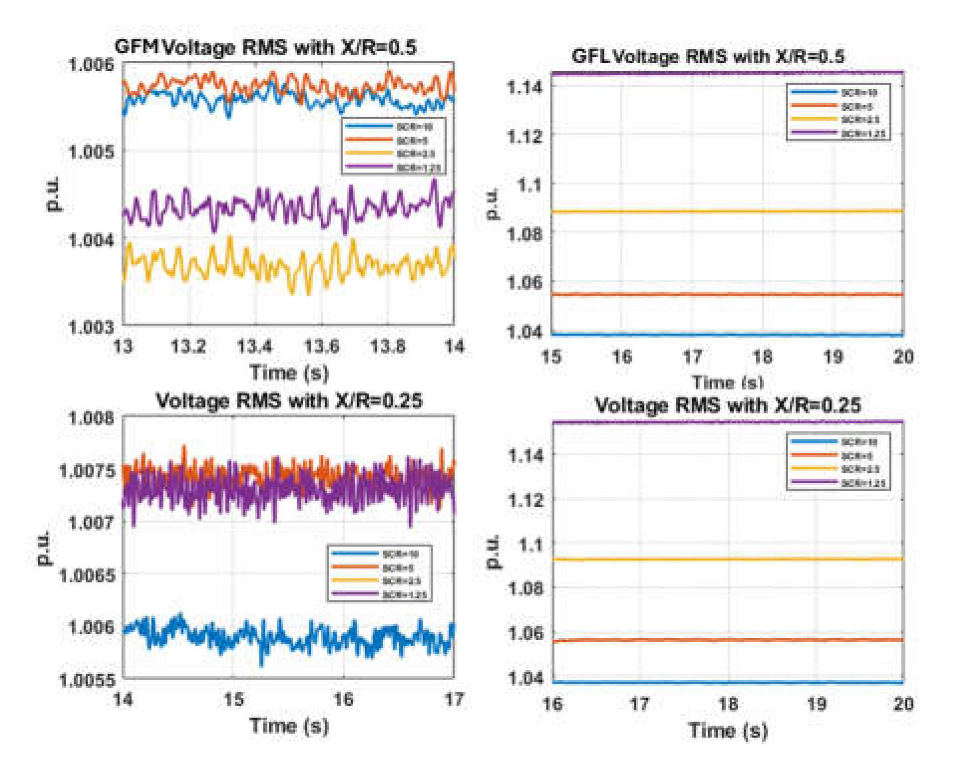
even lower X/R ratio, and the testing results are presented in Figure 5; however, the inverter with GFM control starts to
When in GFM control, I˙= P+j∗Q with P and Q are con-trip with X/R=0.5 and SCR=10. Further, for the rest of trolled by f ∗ and V ∗V ∠θ, respectively. When in GFL control, the tests (X/R=0.5 with SCR=5, 2.5, 1.25 and X/R=0.25 with SCR=10, 5, 2.5, 1.25), the inverters with GFM control all tripped off after approximately 10–15 seconds due to the AC overcurrent; however, the inverter with GFL control did not trip, but the terminal voltage was boosted very high. A deeper look at Figure 5 shows that when the X/R ratio is low (the line impedance becomes more resistive), the inverter with GFM control has difficulty staying connected, and the voltage RMS measurements look very distorted. However, for GFL inverter, the lower X/R (more resistive), the POI voltage is very smoother than higher X/R.
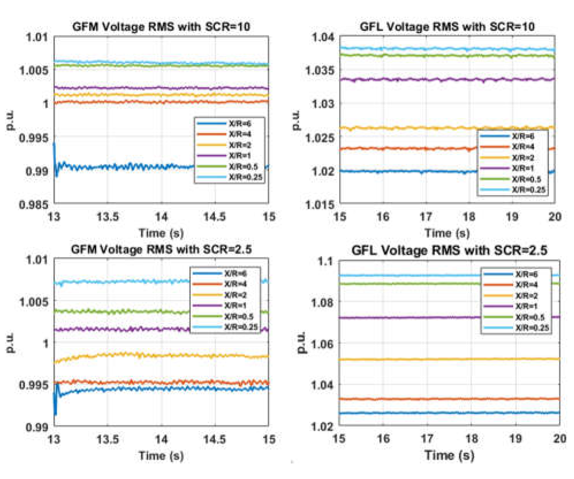
Figure 4 and Figure 5 reveal how different SCRs under varying X/R ratios affect the voltage stability of GFM and GFL inverters. Figure 6 reflects how different X/R under the same SCR affects the voltage stability of GFM and GFL inverters. Note that only the results of SCR=10 and SCR=2.5 are presented due to the limited space of the paper. For the SCR=5, the comparison can be fund in Figure 4 and Figure 5. Under SCR=10, a smaller X/R ratio causes a higher voltage at the terminal of the GFM inverter, and this trend/pattern is also observed for the GFL inverter. This can be understood from the fact that under the same SCR, the lower X/R ratio results in a larger R, which will cause more voltage change (if the inverter injects power into the grid, then there is more
Figure 5.
Varying SCRs under different X/R ratios for GFM control (left) and GFL control (right) with inverter GFM control tripping.
Figure 5.
Varying SCRs under different X/R ratios for GFM control (left) and GFL control (right) with inverter GFM control tripping.
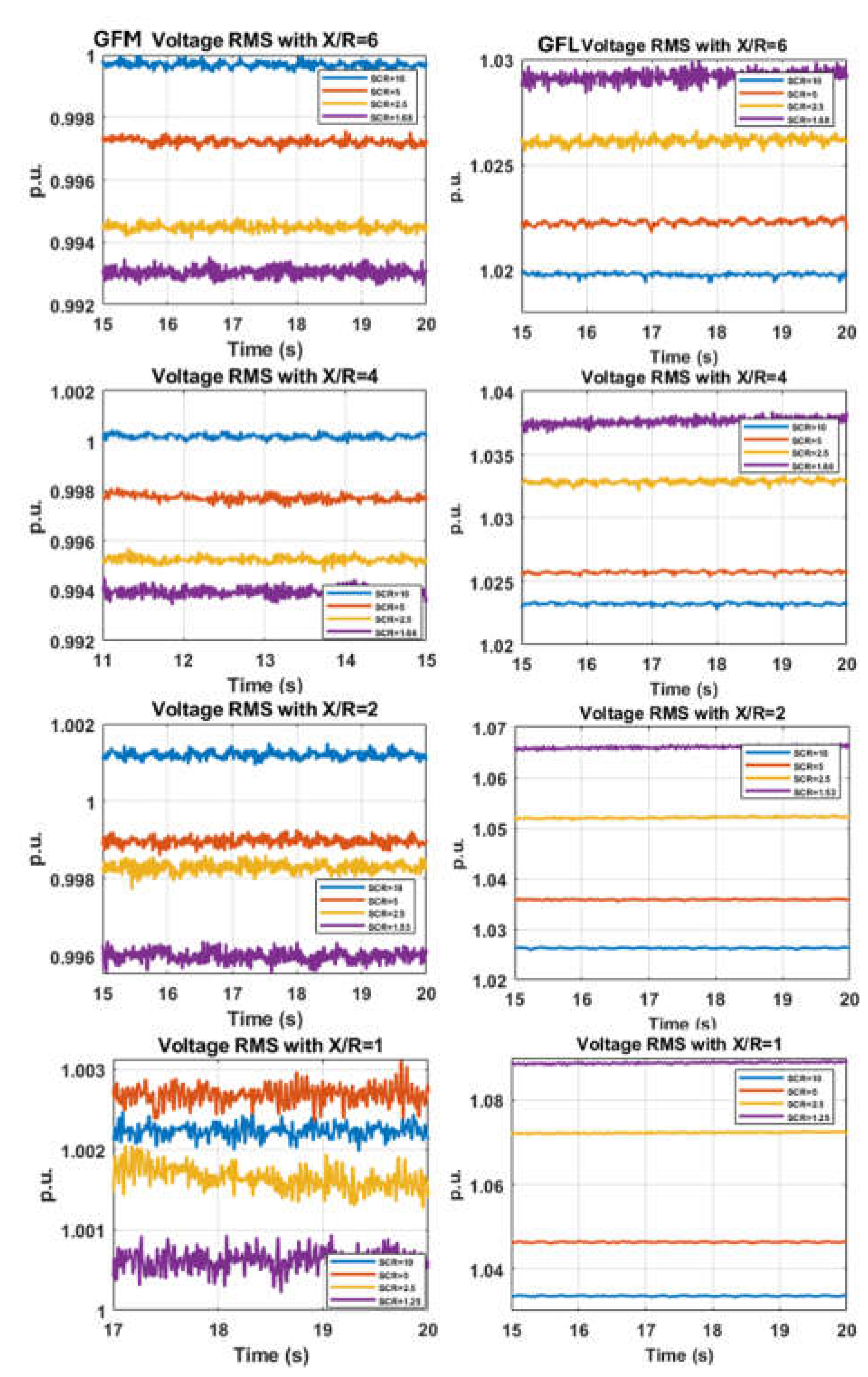
Figure 6. Varying X/R under different SCRs for GFM control (left) and GFL control (right).
voltage rise). Additionally, the voltage should be smoother because the higher resistance can have a damping effect. This is observed for the GFL inverter but not for the GFM inverter. Additionally, we can observe that the GFM inverter maintains the POI voltage very well with both SCR=10 and SCR=2.5 under all different X/R ratios, however, the GFL inverter has good POI voltage with high SCR=10 and causes over- voltage issues with lower SCR=2.5 and lower X/R ratio (from X/R=2 to X/R=0.25).
A. Inverter 2 Testing Results
The hardware test for GFM2 is carried out based on Table III for both GFM and GFL control. The testing results for Inverter 2 with GFM control under varying X/R from 6 to 4, 2, and 1 with changing SCR are presented in Figure 7. Note that Inverter 2 with GFM control starts to trip off when X/R=1, and this is the reason why the results of X/R=0.5 and 0.25 are not presented. For Inverter 2 with GFL control, the inverter also tripped off for all the scenarios listed in Table III when the dispatched active power command is increased from 15% to a higher value (should reach 40% as the GFM control).
Figure 7.
Varying X/R under different SCRs for Inverter 2 with GFM control.
Based on Figure 7 and the unlisted testing results, the main observations are: (1) Inverter 2 has better stability in GFM control mode than GFL control mode under the same SCR and X/R ratios; (2) Inverter 2 with GFM control for the untripped scenarios still shows a similar trend as Inverter 1 with GFM control under the same X/R, where a higher SCR has a higher voltage, and with a reduced X/R, the inverter’s POI voltage increases; (3) compared to Inverter 1 with GFM control, Inverter 2’s voltage stability is worse because the voltage RMS shows oscillations; and (4) the anti-islanding function needs to be disabled or desensitized (less aggressive), otherwise Inverter 2 with GFL control has challenges to synchronize and connect with the grid simulator.
5. Conclusions
This paper evaluates two commercial hardware inverters’ voltage stability under varying grid strengths (SCR and X/R) using a pure hardware setup. The first inverter shows consistent and promising results to draw the trend/pattern of its stability under varying SCRs and X/R; however, the second inverter with GFM control exhibits continuous tripping when the X/R ratio decreases (starts from X/R=1 to 0.5 and 0.25), and it tripped for all the tests with GFL control. The testing results can still indicate that the second inverter works more stably with GFM control than GFL control, and this inverter’s GFM control is able to maintain stability under strong grid conditions (SCR=10 with X/R=6, 4, and 2). This is con- tradictory to the commonly accepted fact that GFM inverters exhibit better stability with a weak grid, not a strong grid. The hardware testing work performed in this paper also tells us that not all inverters behave the same way. More insightful conclusions are drawn from the testing results from the first inverter:
Both X/R and SCR affect the voltage stability of GFM and GFL inverters. X/R affects the voltage stability more than SCR; reducing X/R has a negative impact on the GFM inverter’s stability, whereas it has a positive impact on the GFL’s stability (this indicates that the GFM inverter might have better stability with transmission systems with higher X/R ratios, and GFL inverters might have better stability with distribution systems with lower X/R ratios). Under the same X/R with varying SCRs, the GFM inverter’s POI voltage decreases with a lower SCR, whereas the GFL inverter’s POI voltage increases with a lower SCR.
When the X/R ratio decreases (e.g., X/R=2) with a lower SCR (e.g., SCR=2.5), the GFM inverter is able to maintain the POI voltage profile within the safe operating limits, whereas the GFL inverter usually causes overvoltage issues under the same operating conditions.
The X/R ratio affects the voltage stability of the GFM and GFL inverter differently. When the X/R ratio reduces to very low (e.g., X/R=0.5), the GFM inverter tends to trip off due to the AC overcurrent, and the GFL inverter stays connected but pushes the POI voltage outside the safe operating limits (0.95–1.05 p.u.).
Note that what we observed from the hardware test might be different from analytical studies or simulation re- sults because the hardware inverters usually contain fea- tures/nonlinearities/protection functions that are either not captured or not captured correctly and completely in those studies.
References
- D. Kim, H. D. Kim, H. Cho, B. Park, and L. Byongjun, “Evaluating influence of inverter-based resources on system strength considering inverter interaction level,” Sustainbility, vol. 12, pp. 1–18, 2020.
- Sheth, K. , Patel, D., & Swami, G. (2024). Reducing electrical consumption in stationary long-haul trucks.
- Efficiency, 13(3), Article 6. [CrossRef]
- S. M. Alizadeh, C. S. M. Alizadeh, C. Ozansoy, and T. Alpcan, “The impact of x/r ratio on voltage stability in a distribution network penetrated by wind farms,” in 2016 Australasian Universities Power Engineering Conference (AU- PEC). IEEE, 2016, pp. 1–6.
- R. Yin, Y. R. Yin, Y. Sun, S. Wang, and Z. Lu, “Stability analysis of the grid- tied vsc considering the influence of short circuit ratio and x/r,” IEEE Transactions on Circuits and Systems II: Express Briefs, vol. 69, pp. 129–133, 2022.
- Swami, G. , Sheth, K., & Patel, D. (2025). From ground to grid: The environmental footprint of minerals in renewable energy supply chains.
- Article 2. [CrossRef]
- J. Liu et al., “Impact of power grid strength and pll parameters on stability of grid-connected dfig wind farm,” IEEE Tran. Sustainable Energy, vol. 11, pp. 545–557, 2020.
- C. Henderson, E. A. C. Henderson, E. A. Alvarez, T. Kneuppel, Y. Guangya, and L. Xu, “Grid strength impedance metric: An alternative to scr for evaluating system strength in converter dominated systems,” IEEE Tran. Power Delivery, vol. 39, pp. 386–396, 2024.
- Sheth, K. , & Patel, D. (2024). Strategic placement of charging stations for enhanced electric vehicle adoption in San Diego, California. Journal of Transportation Technologies, 14(1), Article 5.
- jtts. 2024.14 1005.
- L. Huang, C. L. Huang, C. Yang, M. Song, H. Yuan, H. Xie, H. Xin, and Z. Wang, “An adaptive inertia control to improve stability of virtual synchronous machines under various power grid strength,” in 2019 IEEE Power Energy Society General Meeting (PESGM). IEEE, 2019, pp. 1–5.
- Sheth, K. , & Patel, D. (2024). Comprehensive examination of solar panel design: A focus on thermal dynamics.
- 15(1), Article 2. [CrossRef]
- Y. Gu and C. T. Green, “Power system stability with a high penetration of inverter-based resources,” in Proceedings of the IEEE, vol. 111. IEEE, 2027, pp. 832–853.
- Swami, G. , Sheth, K., & Patel, D. (2024). PV capacity evaluation using ASTM E2848: Techniques for accuracy and reliability in bifacial systems. Smart Grid and Renewable Energy, 15(9), Article 12. [CrossRef]
Figure 1.
Laboratory experiment setup.

Figure 2.
The dispatch rule of GFM inverters [11].
Figure 2.
The dispatch rule of GFM inverters [11].
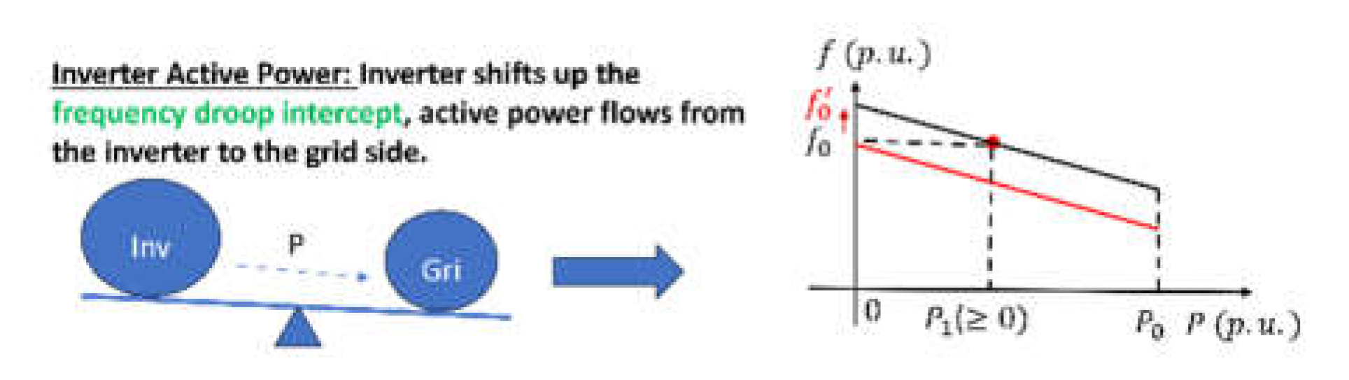
Figure 3.
Phasor diagram analysis of the GFM and GFL inverter for power injection.
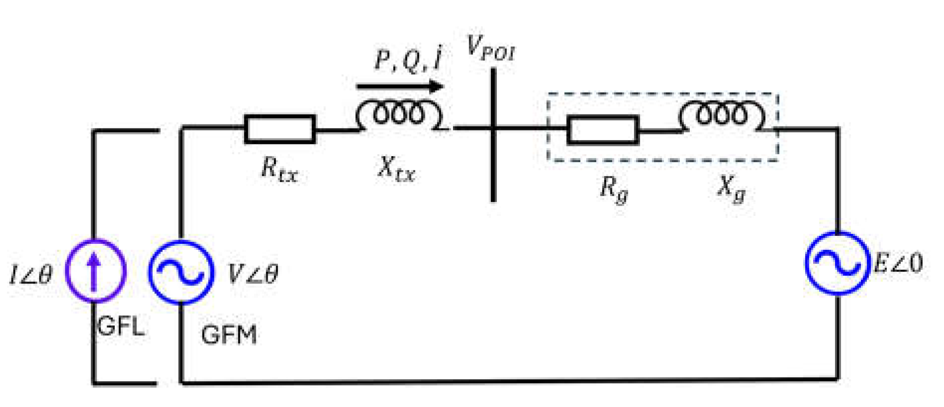
Figure 4.
Varying SCRs under different X/R ratios for GFM control (left) and GFL control (right) with no inverter tripping.
Figure 4.
Varying SCRs under different X/R ratios for GFM control (left) and GFL control (right) with no inverter tripping.
Disclaimer/Publisher’s Note: The statements, opinions and data contained in all publications are solely those of the individual author(s) and contributor(s) and not of MDPI and/or the editor(s). MDPI and/or the editor(s) disclaim responsibility for any injury to people or property resulting from any ideas, methods, instructions or products referred to in the content. |
© 2025 by the authors. Licensee MDPI, Basel, Switzerland. This article is an open access article distributed under the terms and conditions of the Creative Commons Attribution (CC BY) license (http://creativecommons.org/licenses/by/4.0/).
Copyright: This open access article is published under a Creative Commons CC BY 4.0 license, which permit the free download, distribution, and reuse, provided that the author and preprint are cited in any reuse.


