
Submitted:
24 December 2024
Posted:
25 December 2024
You are already at the latest version
Abstract
In the recent years, a continuous effort have been made for modeling and stability analysis of converter dominated grids. Ensuring stability in converter dominated grid presents a unique challenge, primarily due to manufacturers’ intellectual property (IP) protections. Determining the robust stability boundary of a grid incorporating converters from various manufacturers remains an area requiring extensive research. Recently, a grey-box modeling approach for studying interoperability has been proposed in literature. However, the existing methodology is solely suitable for grid following converters. This study bridges the gap by proposing GFM converters model which aligns with the methodology for analyzing interoperability of GFL converters. The model is designed to represent a range of control system implementations across different manufacturers. Using robust control theory, this approach assesses the grid’s stability margin and sensitivity analysis of the uncertain control loops under various conditions considering a single GFM converter. The results are validated both analytically and through real time hardware-in-the-loop (HIL) test to demonstrate the model’s accuracy in predicting robust stability margin and the sensitive of the control loops in GFM converters dominated grids.
Keywords:
Grid-forming
; Grey-box modeling
; Robust stability analysis
; Sensitivity analysis
; Synchronization
; Uncertainty
1. Introduction
Power electronics converters like grid-following (GFL) and grid-forming (GFM) converters are playing a significant roles in integrating renewable energy sources (RESs), e.g., wind power and solar power, into the power grid [1,2]. In addition, the power electronics converters especially the GFM converters are expected to play an important roles in the future multi-terminal high-voltage direct-current (HVDC) transmission systems [3]. Moreover, recent studies on GFM converters are highlighting their significance in the dynamic power sharing between hybrid AC/DC grids. They are mainly used for coupling of low-voltage DC (LVDC) and AC grids, ensuring voltage and current regulation during interconnected and islanding modes. By actively participating in the control of voltage and frequency, these converters enable seamless integration and stabilization of the hybrid grid, ensuring reliable operation under varying load conditions [4,5]. This increasing interests of the transition to the clean energy and the use of the power electronics converters in the multi-terminal HVDC systems and hybrid AC/DC grids, are indeed introducing several challenges to the power system. The first one is stability problem. Power electronics converters which integrate the RES’s to the grid do not inherently provide the same level of inertia as the conventional synchronous generators [6]. This leads to the reduction to the system’s stability of withstanding disturbances [7,8].
The second challenge is interoperability problem due to lack of standardization. The integration of RES and Multi-terminal HVDC system involves the use of power electronics converters from different vendors, each implementing different control algorithms and strategies which may lead to compatibility issues. The control strategies for all of the converters are kept confidential by their manufacturers due to the intellectual property (IP) protection [9]. Converters of different vendors may have a different voltage variations and it might cause unwanted dynamics to the grid unless a proper standardization for converters control system tuning is in place [10].
Grid stability analysis, converters control loop sensitivity analysis, and interoperability analysis of GFM converters are areas for which intense research is needed. However, it requires a precise model which truly represent the GFM converters behaviour. A lot of researches has been conducted to derive model of the converters which can represent the converters behaviour under different operating conditions [11]. The white-box modeling which is based on the assumption that the detailed control structure and parameters of power converters are fully known [12]. This assumption often does not hold true in practice, as industries typically keep the detailed implementation of the converters control system confidential to protect the IP [9].
To address the confidentiality issues, impedance based black-box converter models, which are derived from measurements at their points of connection (PoCs), have gained popularity. These impedance models are accurate only near the nominal operating point used during the estimation process [13]. Given the high variability of load profiles and power injection from renewable sources, modern power systems operate across a wide range of steady state conditions. Unless the measurement is repeated, whenever there is a change in the system’s operating condition, the model would become inaccurate and results a wrong analysis of the power system [9].
Given the confidentiality challenges of white-box modeling and the potential inaccuracy of black-box modeling under change in operating conditions, it is necessary to develop an accurate model of a GFM converters with unknown dynamics for analyzing the robust stability of grids dominated by GFM converters and for establishing converter control tuning guidelines to ensure grid stability. A non-linear grey-box modeling approach has been proposed in [14], but it is only limited to GFL converters. So, this paper is presenting a non-linear grey-box modeling of GFM converters without disclosing the internal details of the converters control system. The model is then used to study the grid’s stability boundary and evaluate the sensitivity of uncertain control loops using robust control theory. In summery in this paper:
- Generic modeling of the GFM converter is provided considering all the possible implementations of: the synchronization, the voltage profile management and the inner voltage and current control loops by assuming only rough and non-detailed knowledge’s of the converter’s control system.
- The generic modeling considers the DC link dynamics, which make it more suitable to model hybrid AC/DC grid.
- A proper definition of uncertainties for each uncertain control loop is discussed to be able to consider all the possible implementations.
- Stability analysis of GFM converters dominated grids using robust control theory is done by studying the stability margin for different operating condition of the grid.
- Sensitivity analysis of the uncertain control loops is also investigated in order to determine which of the control loops have significant impact on the stability of GFM converters dominated grids.
This paper is organized as follows: In section 2, the discussion and modeling of the generic GFM converter is illustrated in detail. In section 3, the grey-box modeling of the GFM converters and the interconnection with power grid has been discussed. In section 4, the robust stability analysis of the grid considering single GFM converter is presented. In section 5, the hard-ware-in-the loop result is presented and in section 6 a brief conclusion has been provided.
2. Power Converters Control System Uncertainties and Their Modeling
Making a few assumptions about the converters control system grounded in understanding of the physical laws governing power converters and their basic operation in power grids, gives a sufficient information to assume the converter as a grey-box rather than viewing it as a black-box model, which would be based solely on impedance-based measurements. For instance, manufacturing industries provide the mode of operations of the converters (e.g. GFL or GFM) and a generic information about their control system as long as it does not reveal confidential details. In addition, the mathematical equations used in power converter models, like energy conservation and reference frame transformations, which are derived from fundamental principles of electromagnetism and standard mathematical techniques are not protected by IP. With the generic information provided by the manufacturing industries without disclosing the internal details, the power converters can be modeled with uncertain control system using grey-box modeling approach.
2.1. Generic Modeling of GFM Converters
In this paper, the generic GFM three phase converter shown in Figure 1 is considered. The control structure of the generic GFM converter consists of a DC voltage control loop , power synchronization loop , the reactive power ac voltage loop , the inner voltage loop and current loop . Due to the possibility of implementing GFM converter control in various ways, the control loops inside the gray-box in Figure 1 are assumed to be unknown and they are modeled through unknown transfer functions , , and . The DC voltage control loop is used to regulate the voltage at the power source, and it is assumed that the control tuning and its implementation is fully known.
The proper modeling of the converter considering its non-linearity is crucial to represent the operating point-dependent behaviors of the converter, which is necessary for system-level small-signal analysis.
2.1.1. Synchronization Loop Modeling
The generic representation of the synchronization loop in the GFM converter is an inclusive representation of all the possible synchronization mechanisms like droop control [15], power synchronization control (PSC) [16], enhanced direct power control (EDPC), synchronverter [17] and synchronous power control (SPC) [18]. The virtual synchronous machine (VSM) swing equation is used to generically represent all the possible implementations of the GFM synchronization mechanisms. So the dynamic equation can be derived as follows:
where J is the virtual inertia, is the damping coefficient, and are the reference active power and the converter active power output, and and are the angular frequency and the synchronization angle.
2.1.2. Reactive Power AC Voltage Loop Modeling
The reactive power injection profile of the grid is dependent on this loop and it is designed based on the grid code requirement. So, a proportional (droop) controller is considered to generically model the reactive power AC voltage loop.
where and are the reference and nominal voltages, and Q and the reactive power output of the converter and the reference reactive power.
2.1.3. Cascaded Voltage and Current Control Loop Modeling
The Integration of the voltage source converters (VSC’s) subsystem to the distribution lines subsystem requires an accurate modeling of the inner voltage and current control loop. The cascaded loop is used to calculate the voltage for producing the pulse width modulation (PWM) signal of the converter.
A wide range of voltage control strategies have been presented in [19] to manage and stabilize the output voltage of GFM converters. These schemes aim to ensure reliable voltage regulation and addressing various operational challenges. For the generic modeling of this loop a cascaded Proportional Integral (PI) controller is considered.
The first control loop which is used to adjust the reference current for the inner current loop based on the difference between the output voltage at the point of common coupling (PCC) and the reference voltage. The corresponding dynamic equation is provided in (5):
where is the reference current of the current controller, is the integral state voltage error and and are the proportional and integral gains of the voltage controller.
The inner current control loop is modeled using impedance modeling approach as in [21], which permits the interconnection of VSCs and distribution lines without the need of virtual resistor.
where is the - axis decoupling term and and are the Proportional and integral gains of the current controller.
Figure 2.
Current loop modeling [22].
Figure 2.
Current loop modeling [22].
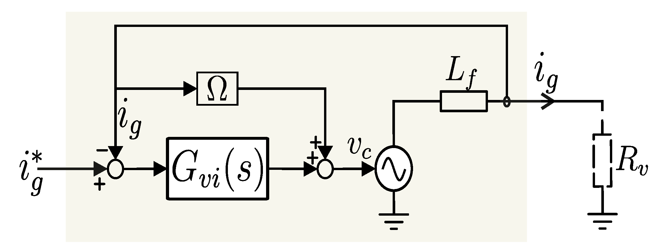
By substituting (8) into (7), the impedance model of the VSC current control loop is derived, as presented in (9). A detailed discussion can be found in [22].
Where is the bandwidth of the current loop. The state space model of the current loop is realized using the non-physical state variables defined by and .
2.1.4. DC Voltage Control Loop Modeling
A Proportional-Integral (PI) controller is employed to regulate the DC input voltage of the GFM converter. The operation of the PI controller is based on the squared difference between the actual DC voltage and the desired DC voltage reference. By minimizing this difference, the PI controller adjusts the current () from the energy sources (e.g. storage systems and wind turbine) to ensure that the DC voltage remains close to its set point. So, the DC voltage control loop is modeled through the dynamic equations as follows:
where is the integral state DC voltage error, and and are the proportional and integral gains of the DC voltage controller. The DC side of the converter dynamics is described by a non-linear power balance equation as in [22][23], by assuming that there is no conversion loss.
2.2. Grey-Box Nonlinear Modeling of GFM Converter
The Grey-box modeling strategy of the GFM converter shown in Figure 1 is illustrated in Figure 3. The model in Figure 3 is composed of the non-linear blocks (in red) and linear blocks (in green). The non-linear dynamics of the DC side of the converter and DC voltage control dynamics indicated in (11), (12) and (14) assumed to be known without uncertainty by assuming that the DC link capacitor and the control turnings for the PI controller are known.
The converter model in Figure 3 presents both input/output for the the ac grid interconnection (, ) and dc interconnection (, ). In the cases of multiple parallel operation of grid connected converters, the frequency of each converter is determined by its local power sharing controller and is modeled using its own local reference frame [24]. So, the transformation of the voltages and currents from global to local frame and vice verse is done through the nonlinear blocks, the direct and inverse rotation matrices and . The matrix is defined as:
and used in the algebraic relations = and = . Clearly, there is no uncertainty on the matrices and , which can thus be considered as known blocks in the converter model in Figure 3.
The remaining blocks in Figure 3 are all linear: the integral relationship is linear and certain, while the transfer functions , and are linear but unknown.
The uncertain control systems of the converter indicated with a green dashed frame in Figure 3 can be modeled by applying frequency dependent uncertainty to the generic representation of the respective control loops by using multiplicative uncertainty principle.
2.3. Multiplicative uncertainty formulation
According to the robust control theory, to model the unknown subsystems the amount of uncertainty of the subsystem must be properly quantified and mathematically characterized [25,26]. The uncertain converter control systems can be modeled by using either additive complex norm-bounded perturbations (additive uncertainty) or linear multiplicative perturbations which are defined in the frequency-domain. Due to its simplicity for robust stability analysis and performance parameters calculation, multiplicative uncertainty modeling [25] is used in this paper.The multiplicative uncertainty is formulated as (16):
where,
- is the real plant transfer function.
- is the transfer function of the nominal control loop implementations. In this case, the control loop parameters and implementations are totally unknown, so the nominal control loop is chosen by the initial guess made with the generic knowledge about the converter.
- is the uncertainty transfer function for which the real plant is deviated from the initial guess . For instance, if a higher deviation is expected in the real implementations of the control loop then can be chosen as a high pass filter. The unknown frequency-dependant transfer function can be defined using a MATLAB command with norm of unitary and can be used to shape the frequency response of the uncertain function.
- is a scalar constant which quantifies the amount of uncertainty.
2.4. Quantitative Design of the Uncertainty in the Converter Control System
The multiplicative uncertainty formulation is now applied to all the uncertain control loops , , and as shown in Figure 3. The definition of the nominal transfer function and the uncertainty is done loop-by-loop, tailored to the individual characteristics and possible implementations of each specific loop.
2.4.1. Synchronization Loop
Various synchronization mechanisms for GFM converters has been presented in different literature’s including droop [15], power synchronization control (PSC) [16], enhanced direct power control (EDPC), synchronverter [17] and synchronous power control (SPC) [18]. The manufacturers generally kept confidential the converters control system and their turnings. In such cases, a nominal plant (i.e. initial guess) for the synchronization loop represented in grey color in Figure 3 is firstly defined, and the unknown dynamics are then included through proper frequency-dependent uncertainty . So as an initial guess , the VSM swing equation is considered:
The uncertainty definition by means of and must be done with several considerations, for the unknown real plant to represent all the possible synchronization loop implementations and their parameter tuning. The relations and equivalency of all those implementations are discussed in [19,20] by properly choosing their parameters. The representation of the synchronization mechanisms are highly different at high frequency ranges so it is reasonable to assume higher uncertainty at high frequency ranges to be able to represent all of them. In the light of this, is chosen 1.5 (150% uncertainty on the nominal plant ) and is chosen to be low at low frequency and high at high frequency. Based on the assumptions made to consider all the possible synchronization loop implementations, the transfer function of the uncertainty is as in (18).
Where, and are chosen to give low uncertainty in the low frequency range and high uncertainty in the high frequency range. The resulting synchronization loop transfer function is shown in Figure 4. The blue curve in Figure 4 is the initial guess of the synchronization loop, while the yellow region in the Bode plot is the admissible region where the frequency response of the real implementation must lay.
2.4.2. Reactive power AC voltage loop
The AC voltage loop is more constrained to the grid reactive power requirement. With a proper knowledge of the grid code it is reasonable to assume no uncertainty in the AC voltage loop in the low frequency range i.e. . At high frequency ranges the response of various controller implementations for AC voltage loop has to be considered. In this paper the nominal AC voltage control loop is modeled with a proportional (droop) constant and known gain.
with the addition of a high-frequency uncertainty, obtained by setting and as a high-pass filter. The resulting transfer function for the reactive power AC voltage loop uncertainty is as in (20) and the uncertain implementation of this control loop lays in the yellow region of the Bode plot shown in Figure 5.
2.4.3. Inner Voltage Control Loop
The primary function of this control loop is to support reactive power to the AC grid. It is therefore, conceived to control the voltage to be as close as possible to the nominal value during grid faults, grid disturbances and over currents. This control loop can be modeled using PI, PR, or virtual admittance models. To encompass all the possible implementations higher uncertainty in high frequency range is considered. The nominal model is with a PI controller tuned with symmetrical optimum technique.
For the uncertain model, the uncertainty is chosen as a high-pass filter without any uncertainty in the low frequency range with the weighting constant . The resulting transfer function for the uncertainty is as in (22) and the uncertain transfer functions of the inner voltage loop implementations lays in the yellow region as depicted in Figure 6.
2.4.4. Inner current control loop
The inner loop is generally designed to have higher bandwidth than the outer loops in order to have a quick response to the change of the command signals. The implementation of this control loop is also by taking in to an account the negative sequence and harmonic compensation schemes. Therefore, higher uncertainty at high frequency ranges and low uncertainty at lower frequency ranges is considered. The generic implementations is a PI controller tuned with technical optimum technique. Therefore, it is modeled as Multiple Input Multiple Output (MIMO) system as in (23)
For the uncertain model, is chosen as a high-pass filter with a slightly lower DC gain in the low-frequency range and the weighting constant . The resulting transfer function of the uncertainty is defined as a MIMO high-pass filter as in (24).
Where, and are chosen to give high uncertainty in the high frequency range and low uncertainty in the low frequency range. The uncertain transfer functions of the inner current loop implementations lays in the yellow region as depicted in Figure 7.
2.4.5. DC voltage control loop
In this paper, the DC voltage control loop is used to control the voltage from the power source (storage system) and it is modeled without uncertainty, which means that and the uncertainty .
3. Nonlinear Grey-Box State-Space Model of Converter-Dominated Grids
The unknown model of the converter’s control system is simply the interconnection of the two blocks: nominal control system and the uncertainty of control systems as shown in Figure 8. This approach is typically used in robust control theory [25,26]to incorporate multiplicative uncertainties in the form (16) by means of Linear Fractional Transformation (LFT). The uncertainty of the control system shown in Figure 8 is defined as MIMO transfer matrix , which is the concatenation of the uncertainties of all control loops as defined in (26).
The remaining blocks of the converter model in Figure 3 that lay outside the dashed green rectangle (dc converter side, rotation matrices and frequency/angle differential relationship) are embedded into the block known nonlinear part, as shown in Figure 8 with red outline. The resulting converter model in Figure 8 is favorable for robust stability analyses since the uncertainty of the control system is interconnected with a fully linear subsystem and the converters non-linear part is isolated and can not be directly affected by the uncertainty.
3.1. Nonlinear Interconnection with the Power Grid
The nonlinear DAE model of the grid is built according to the procedure in [22], and takes the form:
where contains the grid voltage , the reference power and the DC voltage reference and contains the variables used for the power flow analysis (voltage, angle, active and reactive power of the converter). The linearization of (27) requires the computation of the static equilibrium point by solving through Newton-Raphson method.
for a defined and constant input . The total uncertainty does not play any role in the static converters and grid behaviour, but it influences only their transient dynamics. Thus, the uncertainty is considered null () in the nonlinear static model (28) to compute the equilibrium point, and is then included in the grid model only after its linearization.
The computation of through the solution of (28) with the standard Newton-Raphson method is a generalized power flow problem [27]. Once is computed, the steady state power flow variables in are obtained through the non-linear algebraic function . The resulting for a single converter connected to the grid, as in Figure 1, is reported in Table 2 for different values and grid voltage levels .
The model (27) is then linearized around the computed static equilibrium point based on the procedure in [28], obtaining:
The linearized nominal system (29) is then expressed in a frequency domain as . The uncertain grey-box grid model can be then obtained by interconnecting the uncertainty with the nominal grid model using Linear Fractional Transformation (LFT), with the same procedure in [25], which is given by:
with I identity matrix and , i = 1, 2 being the sub-blocks of .
4. Robust Stability Analysis
The first step for the proposed robust stability analysis is the computation of the power grid stability margin in presence of grey-box converter models, defined as:
being the maximum singular value of , which belongs the defined uncertainty set. The solution of (31) is computed through the command in Matlab.
4.1. Robust Stability Analysis of the Grid with Signle GFM Converter
The stability margin of the grid with the considered converter is obtained for different voltage levels under different SCR values as depicted in Figure 9 by considering the parameters in Table 1. In stability analysis, a higher stability margin signifies a greater ability of the system to maintain stability under varying conditions [29]. Therefore, the study of robust stability using stability margin follows the rule "in the context of control loop implementations considering multiplicative uncertainties, the studied system is robustly stable if the stability margin is beyond and oppositely if the stability margin is lower than then the system is not robustly stable". This rule provides a clear benchmark for analyzing the grid’s robust stability analysis with various scenarios.
Applying this rule to the GFM converters dominated power system based on the stability margin values obtained and presented in Figure 9. Considering the case for and , which has a stability margin of , indicating that the GFM converter dominated grid is stable for all possible control tuning included by the uncertainty. This is because, the smallest possible perturbation that is capable of destabilizing this converter-dominated grid system has an norm of that is 197% of the maximum defined admissible perturbation, implies that no destabilizing perturbation exists within the specified range of uncertainty. So, the GFM converters dominated grid system is robustly stable for the considered case for all possible perturbations within the defined range of uncertainties.
For more illustrations let us consider the system for a slightly increased SCR value (for instance for with ), the stability margin which is lower than , This implies that there is at least one destabilizing perturbation with an norm greater than or equal to of the maximum permissible perturbation. Therefore, the system is not robustly stable, as there is at least one unstable control implementation within the specified range of uncertainty. Based on the results obtained the GFM converter-dominated grids become not robustly stable for SCR values greater than due to its robust stability margin result of below .
Due to the non-linearity of the converter model, changing the grid voltage level affects the stability margin values. As clearly seen in Figure 9, the Stability margin decreases with the increase in the grid voltage level. So the injection of reactive power which will increase the grid voltage reduces the stability margin of GFM converters dominated grids. This dependability is because the change in the grid voltage level will also change the equilibrium points computed to linearize the system. Studying this dependency in the impedance based black-box converter modeling is not possible.
Furthermore, the critical frequency value for which instability might occur in the system is also studied and computed through robust stability analysis tools for the scenarios considered for the simulation, and the result is presented in Figure 9. Let us consider the case and , the critical frequency obtained from the simulation is . This implies the frequency at which instability might occur in the system for the considered case is at . Determining the critical frequency is very important to design the damping action without the full knowledge of the grid model during grid resonance instability.
4.2. Sensitivity Analysis of the Control Loops
The sensitivities of robust stability margins concerning each control loop uncertainties were analyzed in percentage to characterize how the variation in normalized perturbations of each control loop affects the grid stability margin. This analysis is necessary because it tells which control loops mainly affect overall system stability under uncertainties and gives insight into the influence of each control loop on the grid stability. The obtained result from the simulation of the model is presented in the Figure 10 for different short circuit ratio values of the grid. For the considered cases, it is found that the reactive power AC voltage and the inner current loop design and tuning have less impact on the stability margin. On the other hand, the synchronization loop and the inner voltage loop tuning have a higher impact on the stability margin.
5. Hardware-in-the-Loop (HIL) Result
In order to validate the robust stability analysis result obtained by robust control theory, the power grid in Figure 1 simulated in a real time simulation tool, Typhoon HIL device. The validation of the generic model is firstly done to ensure if it can exactly reflects the behaviors of GFM converters and followed by verification of robust stability analysis results.
5.1. Model Validation with HIL Real Time Simulation
To ensure the accuracy of the results from the robust stability analysis, it is essential to verify that the mathematical model developed in Section 2 accurately reflects the behavior of GFM converters. Due to the sense of generality of the model of the converter, the validation is done with two control system implementation of GFM converters i.e. Droop and VSM.
The dynamic response for each converter case is compared with the HIL result. As can be seen in Figure 11, during a voltage sag, the GFM converters attempt to compensate the drop by adjusting their output voltage, providing voltage support to prevent further sag. The current wave forms indicates that there is an increase in leading current to inject the necessary reactive power to the grid to compensate the voltage drop and restore the voltage level and stability of the grid.
5.2. Robust Stability Analysis Validation
In order to validate the results obtained by the robust control theory, two converters with different control mechanisms are considered for the analysis: one utilizing VSM control and the other employing droop control. These control systems of the converters are accurately represented by the generic representation of the GFM in Section 2.
The result in Figure 12 is obtained by considering VSM controlled GFM and droop controlled GFM, with SCR of 3.5. In this case the grid is stable regardless of which converter cases are integrated with the grid. The grid is subjected to a voltage sag of for , the stability is preserved even though a disturbance happens in the grid. This demonstrates that the grids for which the GFM converters connected with it are stable for week grid conditions regardless of the various possible control implementations. Differently, the result shown in Figure 13 is obtained by setting the SCR equal to 4. As shown in the figure the stability is preserved for droop controlled GFM during transient but instability is observed in the response of VSM controlled GFM. This implies stability is not warranted for GFM converter dominated grids when the SCR is greater than 3.5. So, based on the results from the robust stability analysis and the HIL implementation, stability of weak grid is ensured when GFM converters are connected with it. Further increase in the short circuit ratio of the grid causes a stability problem.
Therefore, robust stability of the grid for which GFM converters connected with it are ensured for SCR value of 3.5 or lower, which aligns with the results obtained with robust control theory analyzed by using the generic model discussed in Section 2.
To verify the sensitivity analysis result of which control loop tuning is playing a significant role in the stability of GFM converters dominated grids, a real time simulation is done considering two tuning cases as defined in Table 3. The result in Figure 14 indicated by orange colour is obtained by using the case Tuning A, for which the synchronization and the inner voltage loop are tuned, while the reactive power AC voltage loop and the inner current loop remain unchanged from their initial settings. In this case the stability of the grid is significantly distorted, underscoring the critical role of precise tuning in both the synchronization and inner voltage loops in the stability of the grid. Differently, the result indicated by green colour in Figure 14 is demonstrating the second case Tuning B, where the reactive power AC voltage loop and the inner current loop are tuned, and the synchronization and the inner voltage loop remain unchanged from their initial settings. In this case the effect in the stability of the grid is insignificant, implying the reactive power AC voltage loop and the inner current loop tuning does not play a significant role in the stability of the GFM converters dominated grids.
6. Conclusions
This paper presented, a grey-box model of GFM converter without disclosing the internal details of the converters control system. Robust control theory is utilized to study the robust stability boundary of the grid with GFM converters connected to it. Based on the results obtained, the GFM converters dominated grid is robustly stable for SCR values below 3.5. However, stability is not warranted for SCR values exceeding 3.5, this is because the stability margin is below for large SCR values. In addition, sensitivity analysis of the control loops is also done to give an intuition on which control loop tuning is playing a significant role in the stability of GFM converters dominated grids. To demonstrate this, the bandwidths of the synchronization and the inner voltage loop, and the reactive power AC voltage loop and inner current loop are reduced to below of their nominal value alternatively. It has been found that the synchronization and the inner voltage loop are significantly affecting the stability of the grid, while the tuning of the reactive power AC voltage loop and inner current loop have a negligible effect on grid stability. So, from control loop tuning point of view to avoid grid instability, with this modeling approach system operators can compute and deliver stability specifications to converter manufacturers in the forms of a set of tuning boundaries for the control loops which ensures grid stability. In order to verify the results a real time simulation with Typhoon HIL is performed and it has been demonstrated that the results in both MATLAB and HIL simulation are consistent.
References
- Hesam Pishbahar, Frede Blaabjerg, Hedayat Saboori, Emerging grid-forming power converters for renewable energy and storage resources integration – A review, Sustainable Energy Technologies and Assessments, Volume 60, 2023, 103538, ISSN 2213-1388, https://doi.org/10.1016/j.seta.2023.103538. [CrossRef]
- H. Zhang, W. Xiang, W. Lin and J. Wen, "Grid Forming Converters in Renewable Energy Sources Dominated Power Grid: Control Strategy, Stability, Application, and Challenges," in Journal of Modern Power Systems and Clean Energy, vol. 9, no. 6, pp. 1239-1256, November 2021, doi: 10.35833/MPCE.2021.000257. [CrossRef]
- Y. Liao, H. Wu, X. Wang, M. Ndreko, R. Dimitrovski and W. Winter, "Stability and Sensitivity Analysis of Multi-Vendor, Multi-Terminal HVDC Systems," in IEEE Open Journal of Power Electronics, vol. 4, pp. 52-66, 2023, doi: 10.1109/OJPEL.2023.3234803. [CrossRef]
- J. Arévalo-Soler, M. Nahalparvari, D. Groß, E. Prieto-Araujo, S. Norrga and O.Gomis-Bellmunt, "Small-Signal Stability and Hardware Validation of Dual-Port Grid-Forming Interconnecting Power Converters in Hybrid AC/DC Grids," in IEEE Journal of Emerging and Selected Topics in Power Electronics, doi: 10.1109/JESTPE.2024.3454992. [CrossRef]
- Á. Navarro-Rodríguez, P. García, C. Gómez-Aleixandre and C. Blanco, "Cooperative Primary Control of a Hybrid AC/DC Microgrid Based on AC/DC Virtual Generators," in IEEE Transactions on Energy Conversion, vol. 37, no. 4, pp. 2837-2850, Dec. 2022, doi: 10.1109/TEC.2022.3203770. [CrossRef]
- Pengfei Hu, Yujing Li, Yanxue Yu, Frede Blaabjerg, Inertia estimation of renewable-energy-dominated power system, Renewable and Sustainable Energy Reviews, Volume 183, 2023, 113481, ISSN 1364-0321, https://doi.org/10.1016/j.rser.2023.113481. [CrossRef]
- S. Saha, M.I. Saleem, T.K. Roy, Impact of high penetration of renewable energy sources on grid frequency behaviour, International Journal of Electrical Power & Energy Systems, Volume 145, 2023,108701, ISSN 0142-0615, https://doi.org/10.1016/j.ijepes.2022.108701. [CrossRef]
- Majid Mehrasa, Edris Pouresmaeil, Amir Sepehr, Bahram Pournazarian, João P.S. Catalão, Control of power electronics-based synchronous generator for the integration of renewable energies into the power grid, International Journal of Electrical Power & Energy Systems, Volume 111, 2019, Pages 300-314, ISSN 0142-0615, https://doi.org/10.1016/j.ijepes.2019.04.016. [CrossRef]
- Y. Liao, Y. Li, M. Chen, L. Nordstr¨om, X. Wang, P. Mittal, and H. V. Poor, “Neural network design for impedance modeling of power electronic systems based on latent features,” IEEE Transactions on Neural Networks and Learning Systems, pp. 1–13, 2023.
- A. Suryani, I. Sulaeman, O. A. Rosyid, N. Moonen and J. Popović, "Interoperability in Microgrids to Improve Energy Access: A Systematic Review," in IEEE Access, vol. 12, pp. 64267-64284, 2024, doi: 10.1109/ACCESS.2024.3396275. [CrossRef]
- M. Paolone, T. Gaunt, X. Guillaud, M. Liserre, S. Meliopoulos, A. Monti, T. Van Cutsem, V. Vittal, and C. Vournas, “Fundamentals of power systems modelling in the presence of converter interfaced generation,” Electric Power Systems Research, vol. 189, p. 106811, 2020.
- M. Rasheduzzaman et al., “Reduced-order small-signal model of microgrid systems,” IEEE Trans on Sust. En., vol. 6, no. 4, pp. 1292–1305, Oct. 2015.
- A. Riccobono, M. Mirz, and A. Monti, “Noninvasive online parametric identification of three-phase ac power impedances to assess the stability of grid-tied power electronic inverters in lv networks,” IEEE Journal of Emerging and Selected Topics in Power Electronics, vol. 6, no. 2, pp. 629–647, 2018.
- Federico Cecati, Marco Liserre. Interoperability Specifications for Multi Vendor Converter-Dominated Grid: a Robust Stability Perspective. TechRxiv. October 28, 2024. DOI: 10.36227 techrxiv.173014688.86172997/v1.
- Sana Fazal et al. ‘Droop control techniques for grid forming inverter’. In: 2022 IEEE PES 14th Asia-Pacific Power and Energy Engineering Conference (APPEEC). IEEE. 2022, pp. 1–6.
- Zhang, L.; Harnefors, L.; Nee, H.-P. Power-Synchronization Control of Grid Connected Voltage-Source Converters. IEEE Trans. Power Syst. 2010, 25, 809–820.
- Qing-Chang Zhong et al. ‘Self-synchronized synchronverters: Inverters without a dedicated synchronization unit’. In: IEEE Transactions on power electronics 29.2 (2013), pp. 617–630.
- P. Rodríguez, C. Citro, J. I. Candela, J. Rocabert and A. Luna, "Flexible Grid Connection and Islanding of SPC-Based PV Power Converters," in IEEE Transactions on Industry Applications, vol. 54, no. 3, pp. 2690-2702.
- R. Rosso, X. Wang, M. Liserre, X. Lu and S. Engelken, "Grid-Forming Converters: Control Approaches, Grid-Synchronization, and Future Trends—A Review," in IEEE Open Journal of Industry Applications, vol. 2, pp. 93-109, 2021, doi: 10.1109/OJIA.2021.3074028. [CrossRef]
- Salvatore D’Arco and Jon Are Suul. ‘Equivalence of virtual synchronous machines and frequency droops for converter-based microgrids’. In: IEEE Transactions on Smart Grid 5.1 (2013), pp. 394–395.
- F. Cecati, R. Zhu, M. Liserre and X. Wang, "State-feedback-based Low-Frequency Active Damping for VSC Operating in Weak-Grid Conditions," 2020 IEEE Energy Conversion Congress and Exposition (ECCE), Detroit, MI, USA, 2020, pp. 4762-4767, doi: 10.1109 ECCE44975.2020.9235338.
- F. Cecati, R. Zhu, M. Liserre and X. Wang, "Nonlinear Modular State-Space Modeling of Power-Electronics-Based Power Systems," in IEEE Transactions on Power Electronics, vol. 37, no. 5, pp. 6102-6115, May 2022, doi: 10.1109/TPEL.2021.3127746. [CrossRef]
- Teodorescu, R., Liserre, M., & Rodriguez, P. (2011). Grid converters for photovoltaic and wind power systems. John Wiley & Sons.
- Nagaraju Pogaku, Milan Prodanovic and Timothy C Green. ‘Modeling, analysis and testing of autonomous operation of an inverter-based microgrid’. In: IEEE Transactions on power electronics 22.2 (2007), pp. 613–625.
- Kemin Zhou and John Comstock Doyle. Essentials of robust control. Vol. 104. Prentice hall Upper Saddle River, NJ, 1998.
- Sigurd Skogestad and Ian Postlethwaite. Multivariable feedback control: analysis and design. john Wiley & sons, 2005.
- F. Milano, "An open source power system analysis toolbox," in IEEE Transactions on Power Systems, vol. 20, no. 3, pp. 1199-1206, Aug. 2005, doi: 10.1109/TPWRS.2005.851911 . [CrossRef]
- F. Cecati, R. Zhu, M. Langwasser, M. Liserre and X. Wang, "Scalable State-Space Model of Voltage Source Converter for Low Frequency Stability Analysis," 2020 IEEE Energy Conversion Congress and Exposition (ECCE), Detroit, MI, USA, 2020, pp. 6144-6149, doi: 10.1109/ECCE44975.2020.9236020. [CrossRef]
- F. Cecati, M. Andresen, R. Zhu, Z. Zou and M. Liserre, "Robustness Analysis of Voltage Control Strategies of Smart Transformer," IECON 2018 - 44th Annual Conference of the IEEE Industrial Electronics Society, Washington, DC, USA, 2018, pp. 5566-5573, doi: 10.1109/IECON.2018.8591116. [CrossRef]
Figure 1.
Generic representation of GFM converter with power synchronization loop, reactive power ac voltage loop, inner voltage loop and current loop.
Figure 1.
Generic representation of GFM converter with power synchronization loop, reactive power ac voltage loop, inner voltage loop and current loop.
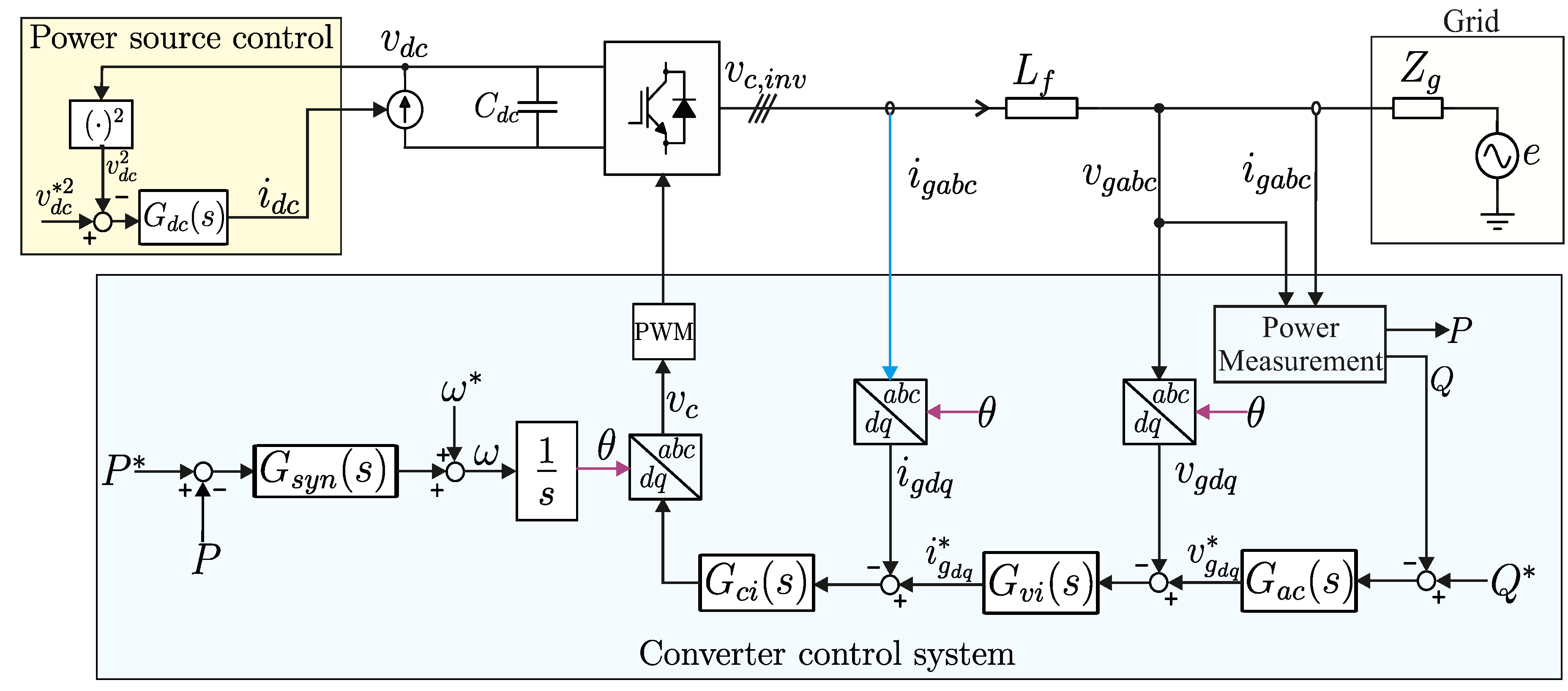
Figure 3.
The proposed modeling scheme for the generic GFM converter including linear, nonlinear, and uncertain blocks.
Figure 3.
The proposed modeling scheme for the generic GFM converter including linear, nonlinear, and uncertain blocks.
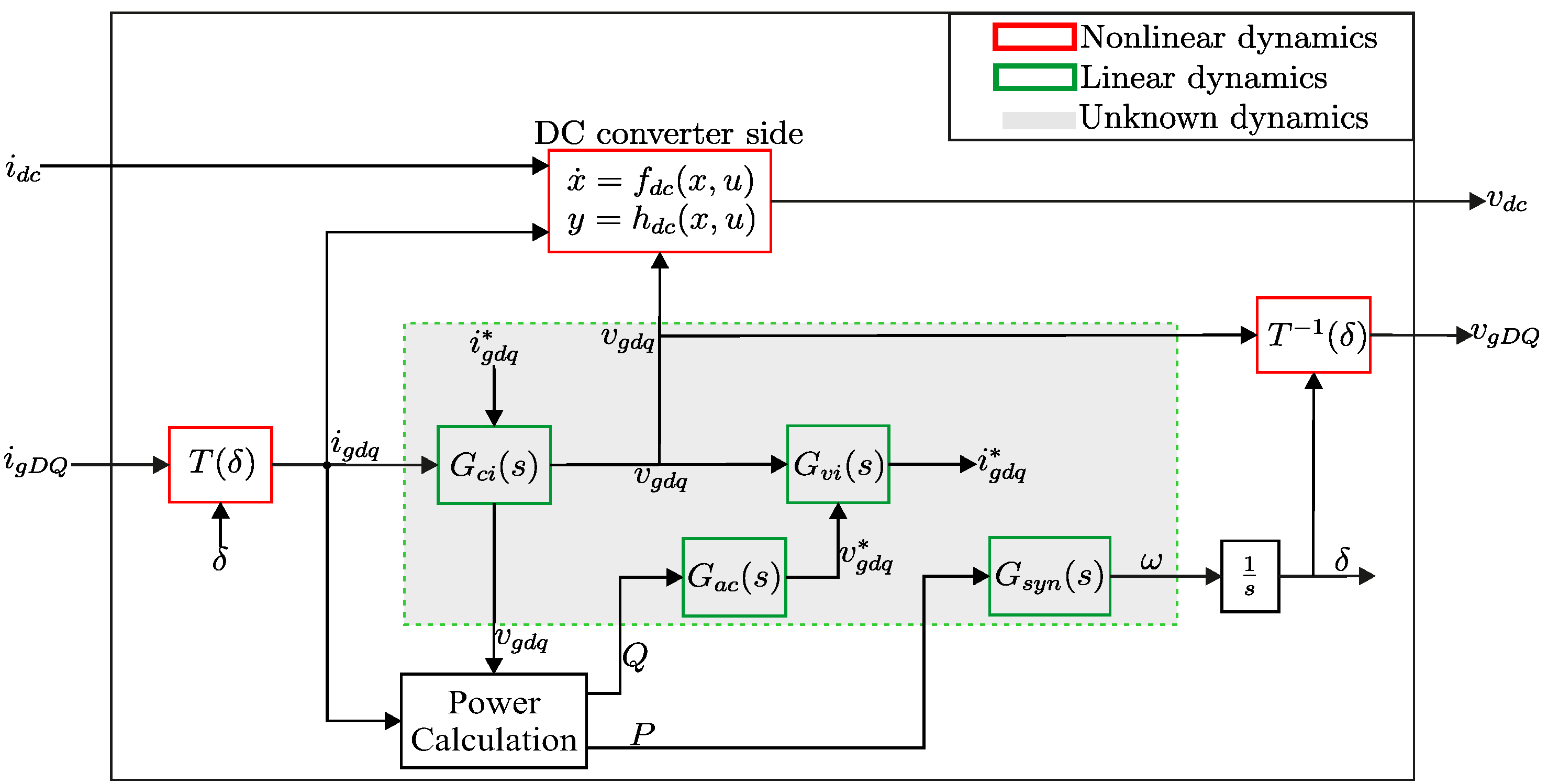
Figure 4.
The uncertain frequency response of the synchronization loop.
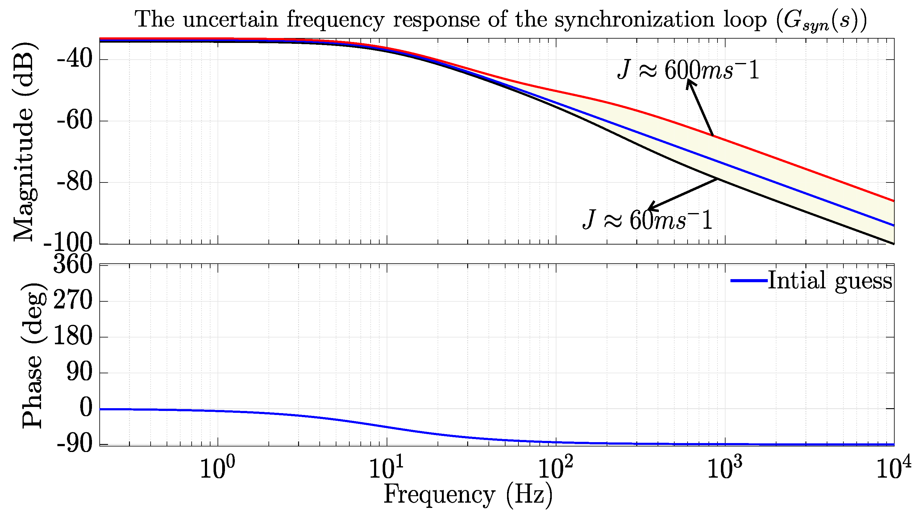
Figure 5.
The uncertain frequency response of the reactive power AC voltage loop.
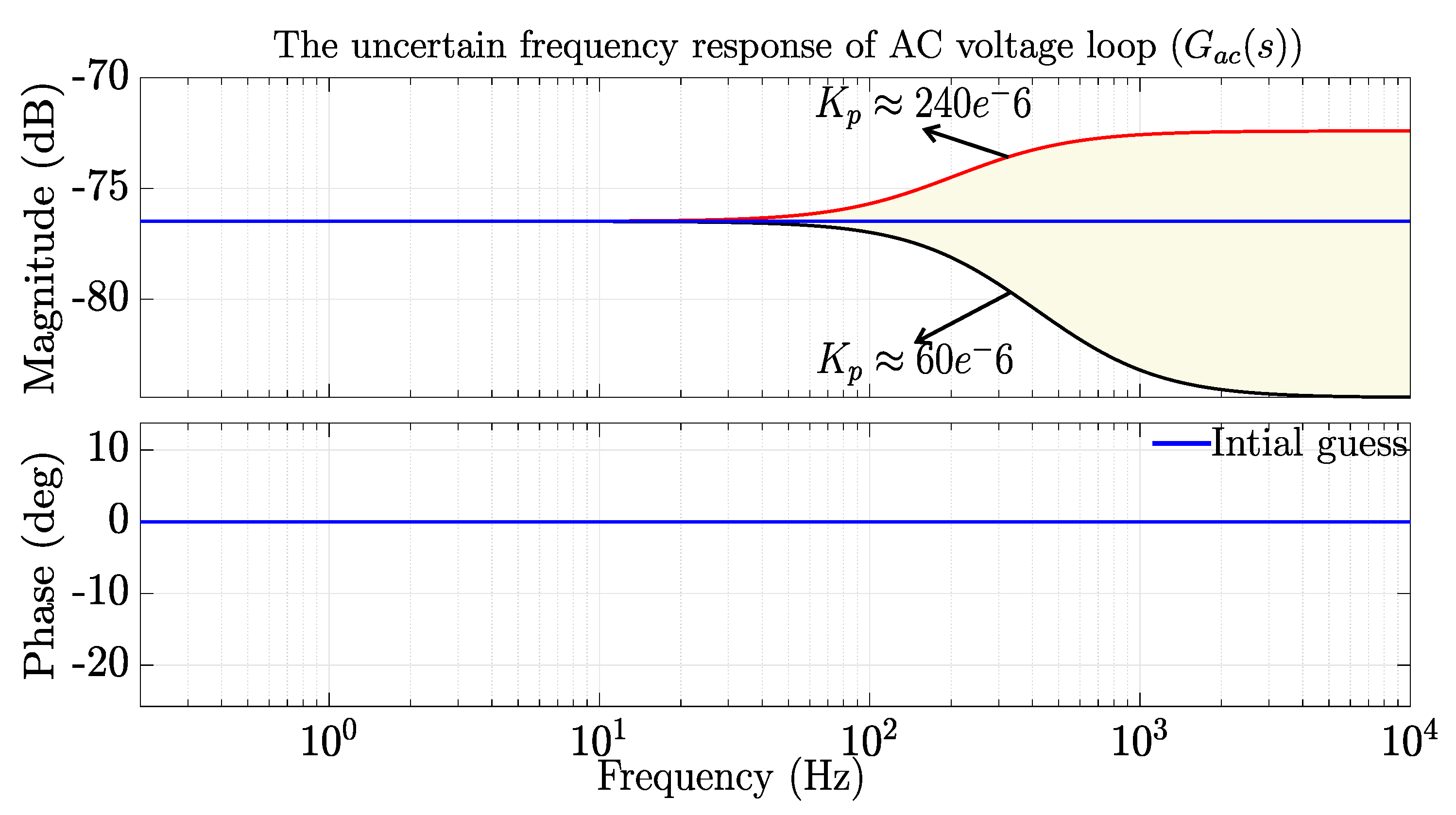
Figure 6.
The uncertain frequency response of the inner voltage loop.
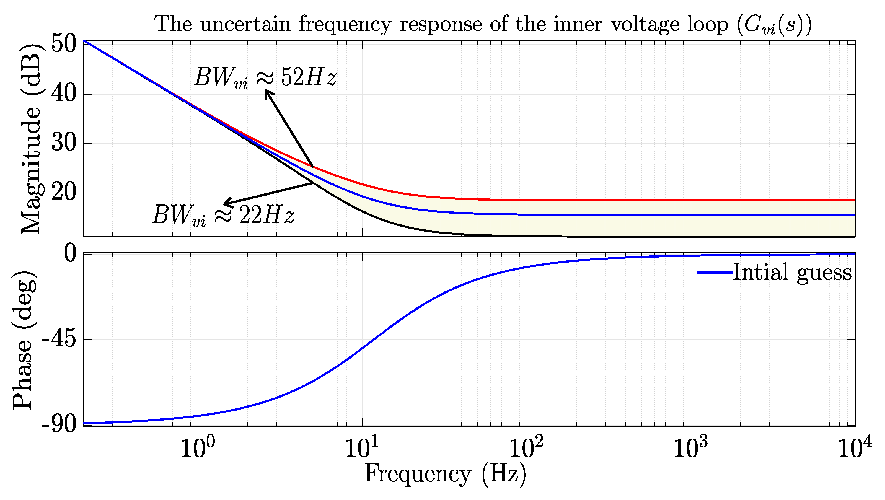
Figure 7.
The uncertain frequency response of the inner current loop.
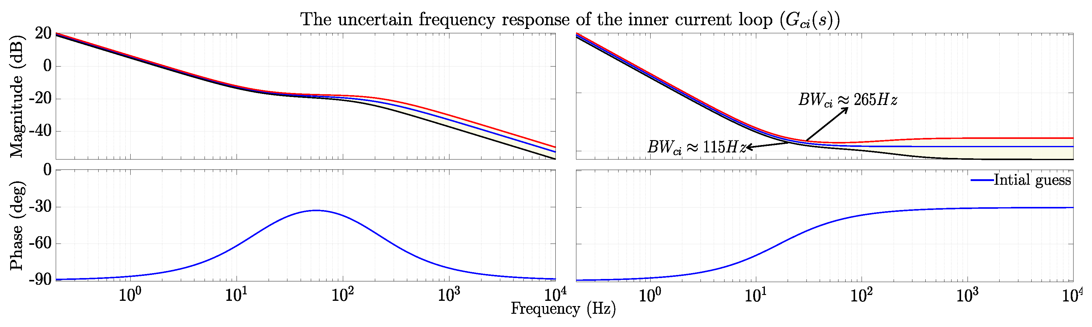
Figure 8.
The block interconnection procedure to embed the uncertainty in the proposed grey-box nonlinear converter model.
Figure 8.
The block interconnection procedure to embed the uncertainty in the proposed grey-box nonlinear converter model.
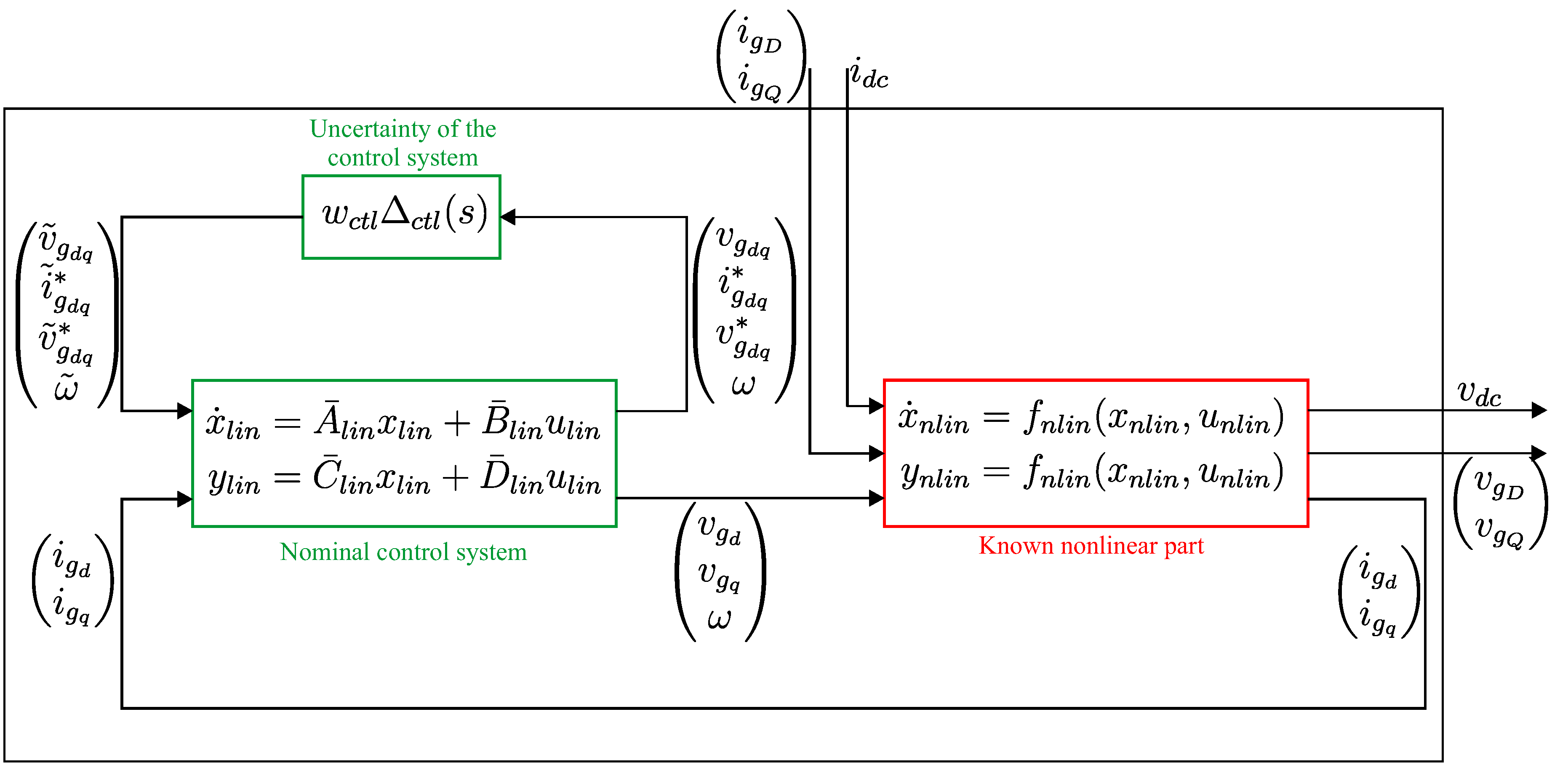
Figure 9.
Robust stability analysis results for different SCR and grid voltage values: (a) Stability margin and (b) Critical frequency.
Figure 9.
Robust stability analysis results for different SCR and grid voltage values: (a) Stability margin and (b) Critical frequency.
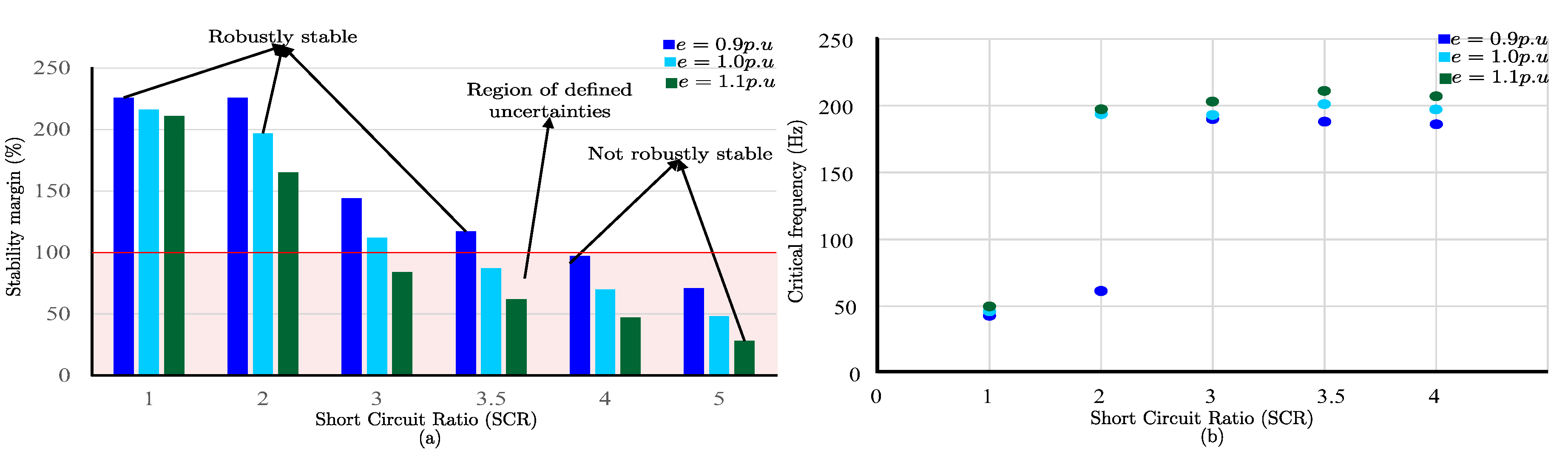
Figure 10.
The sensitivity of the robust stability margin with respect to the individual control loops uncertainty.
Figure 10.
The sensitivity of the robust stability margin with respect to the individual control loops uncertainty.
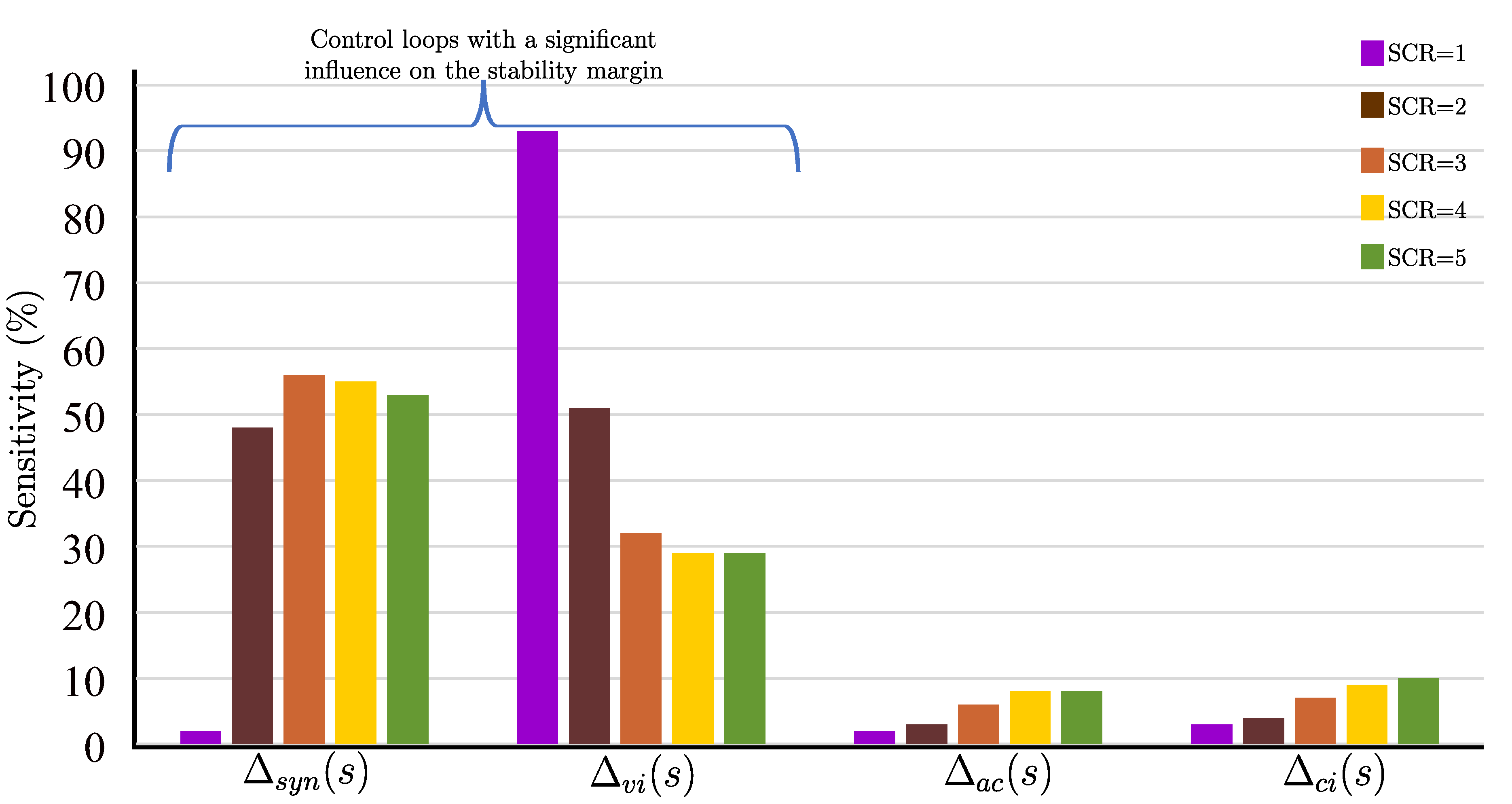
Figure 11.
The validation of the proposed GFM converter model with respect to: (a) Droop controlled GFM converter and (b) VSM controlled GFM converter.
Figure 11.
The validation of the proposed GFM converter model with respect to: (a) Droop controlled GFM converter and (b) VSM controlled GFM converter.
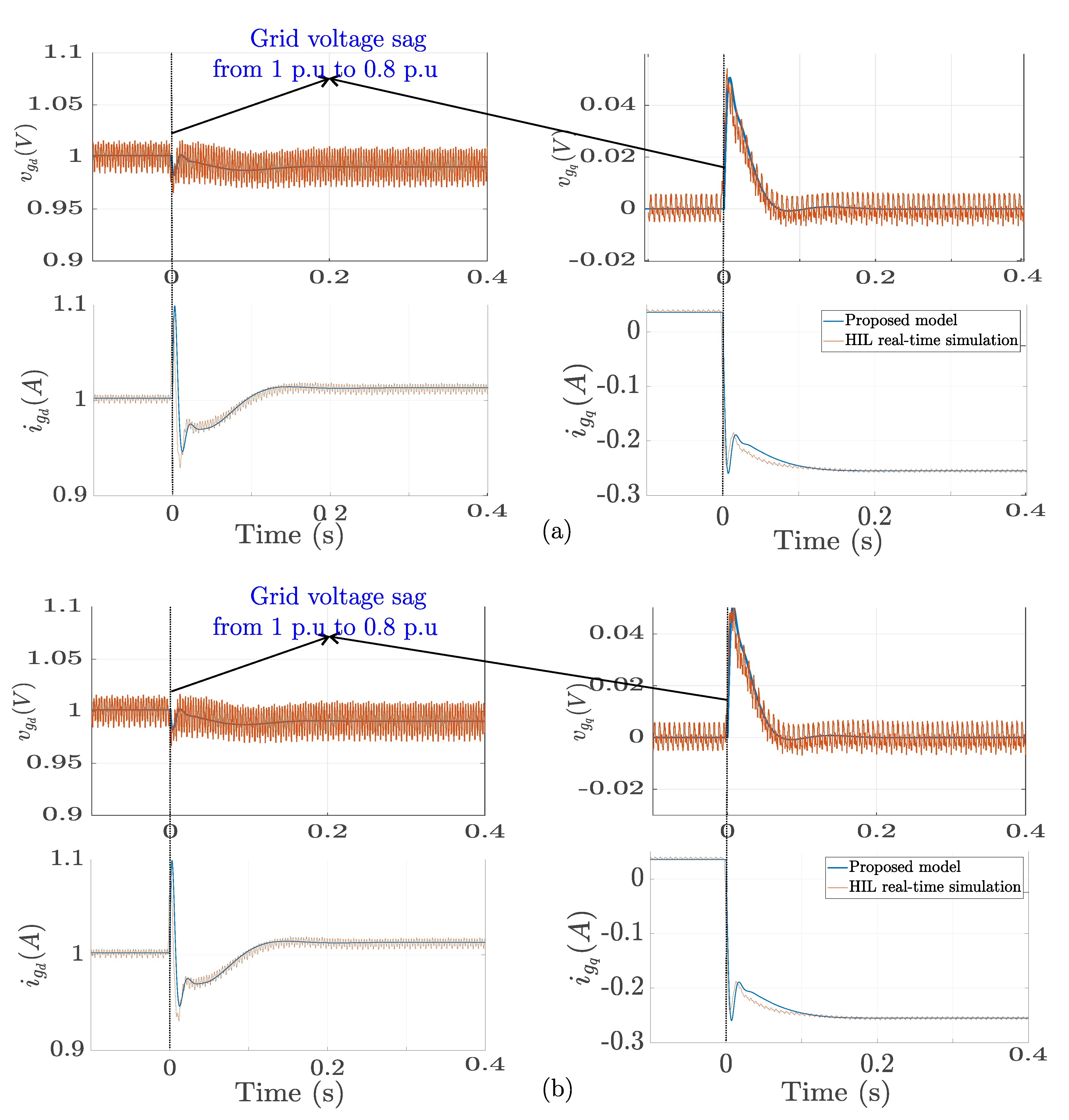
Figure 12.
The real-time HIL simulation of the grid connected to GFM converter of different control systems with .
Figure 12.
The real-time HIL simulation of the grid connected to GFM converter of different control systems with .
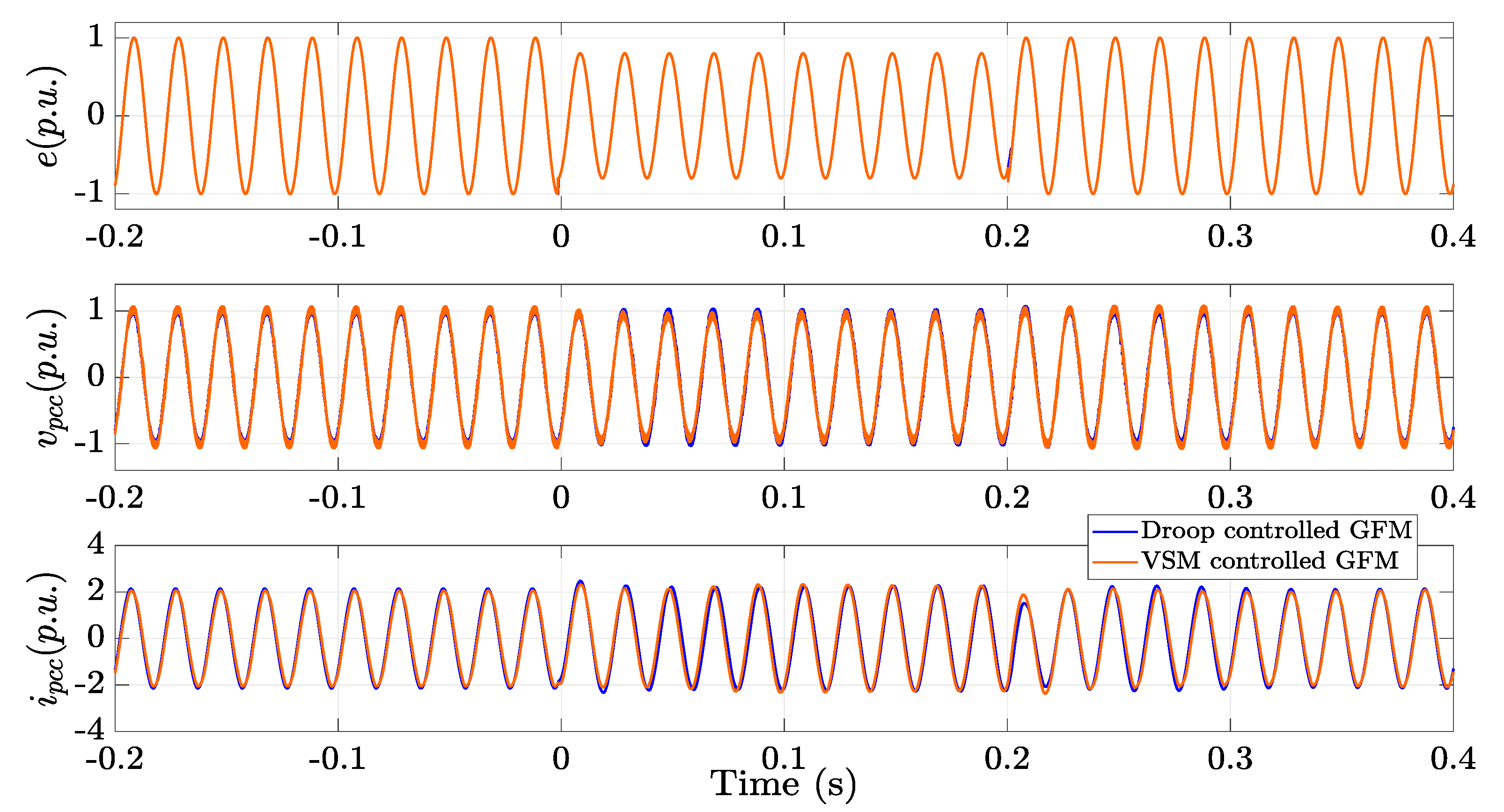
Figure 13.
The real-time HIL simulation of the grid connected to GFM converter of different control systems with .
Figure 13.
The real-time HIL simulation of the grid connected to GFM converter of different control systems with .
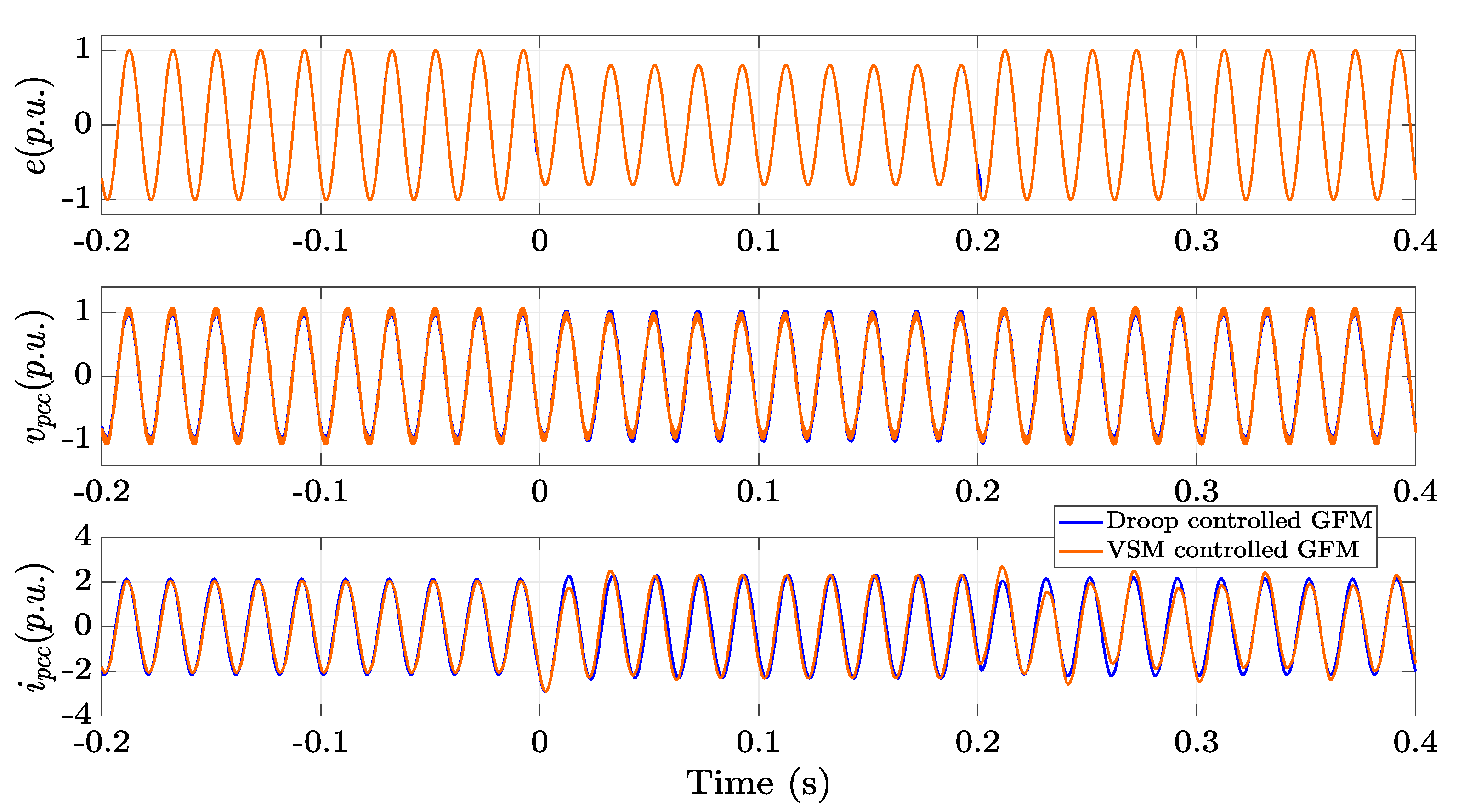
Figure 14.
The real-time HIL simulation of the grid with different control loop tunings: the response of Tuning A is indicated by orange colour and Tuning B is indicated by green colour.
Figure 14.
The real-time HIL simulation of the grid with different control loop tunings: the response of Tuning A is indicated by orange colour and Tuning B is indicated by green colour.
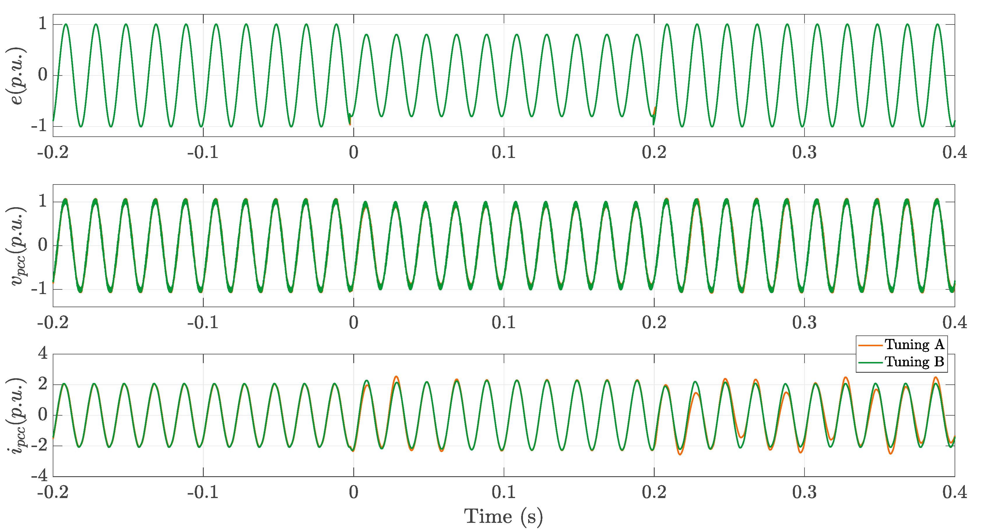

Table 1.
Parameters considered for robust stability (RS) analysis.
| Grid and converter parameters | Nominal values | For RS Analysis |
|---|---|---|
| Line-to-line grid voltage (V) | 690 | 690 |
| Short Circuit Ratio | 1.5 | variable |
| R/X ratio | 0.4 | 0.4 |
| DC-link capacitor (mF) | 22 | 22 |
| Converters Control Parameters | Nominal values | For RS Analysis |
| Active power reference (MW) | 1 | 1 |
| Switching frequency (kHz) | 2 | 2 |
| DC-link voltage reference (V) | 1100 | 1100 |
| DC voltage time constant (ms) | 100 | 100 |
| AC voltage controller gain | unknown | |
| Bandwidth of the synchronization loop (rad/s) | 540 | unknown |
| Bandwidth of the inner voltage loop (rad/s) | 460 | unknown |
| Bandwidth of the inner current loop (rad/s) | 1200 | unknown |
Table 2.
Equilibrium point of the single converter under different SCR’s and grid voltage steady state values.
Table 2.
Equilibrium point of the single converter under different SCR’s and grid voltage steady state values.
| Steady-state var. | |||||
|---|---|---|---|---|---|
| 0.91 | 0.986 | 0.987 | 0.981 | ||
| 0.9 | 39.79 | 15.42 | 10 | 7.41 | |
| 1 | 1 | 1 | 1 | ||
| 0.33 | 0.052 | 0.049 | 0.07 | ||
| 0.958 | 1.024 | 1.032 | 1.033 | ||
| 1 | 32.7 | 14.02 | 9.17 | 6.83 | |
| 1 | 1 | 1 | 1 | ||
| 0.158 | -0.089 | -0.122 | -0.125 | ||
| 0.993 | 1.06 | 1.08 | 1.088 | ||
| 1.1 | 28.68 | 12.89 | 8.5 | 6.35 | |
| 1 | 1 | 1 | 1 | ||
| 0.027 | -0.235 | -0.30 | -0.33 |
Table 3.
Control loop tunings for sensitivity analysis.
| Control systems | Initial guess | Tuning A | Tuning B |
|---|---|---|---|
| AC voltage controller gain | |||
| Bandwidth of the inner current loop (rad/s) | 1200 | 1200 | 445 |
| Bandwidth of the synchronization loop (rad/s) | 540 | 200 | 540 |
| Bandwidth of the inner voltage loop (rad/s) | 460 | 170 | 460 |
Disclaimer/Publisher’s Note: The statements, opinions and data contained in all publications are solely those of the individual author(s) and contributor(s) and not of MDPI and/or the editor(s). MDPI and/or the editor(s) disclaim responsibility for any injury to people or property resulting from any ideas, methods, instructions or products referred to in the content. |
© 2024 by the authors. Licensee MDPI, Basel, Switzerland. This article is an open access article distributed under the terms and conditions of the Creative Commons Attribution (CC BY) license (http://creativecommons.org/licenses/by/4.0/).
Copyright: This open access article is published under a Creative Commons CC BY 4.0 license, which permit the free download, distribution, and reuse, provided that the author and preprint are cited in any reuse.


