A Multiperiod Optimization Framework for Portfolio Selection Using Interval Analysis

1. Introduction

Portfolio selection theory has its roots in the seminal work of Markowitz [16], where asset return is measured as the mean and risk as the variance. Over the decades, classical approaches such as the mean–variance and mean–variance–skewness models [2,20] have served as cornerstones of modern portfolio theory. These models, however, rely heavily on the availability of precise probabilistic information—a condition rarely satisfied in practice. In real-world markets, particularly in emerging or highly volatile sectors, data scarcity, non-stationarity, and limited liquidity often invalidate the assumptions of normality and stationarity upon which traditional models depend [3,21].

Furthermore, these traditional frameworks tend to oversimplify investor behavior by reducing complex preferences to two criteria—expected return and risk—neglecting aspects such as liquidity constraints, market friction, and informational incompleteness. As investor expectations evolve and markets grow more turbulent, the necessity for models that acknowledge and incorporate such real-world imperfections becomes increasingly evident [5,7]. To address these limitations, our study adopts interval analysis as a robust and flexible alternative to probabilistic and fuzzy set approaches [1,4,9]. Within this framework, key variables such as return, risk, and liquidity are modeled as interval-valued parameters. This formulation accounts for bounded uncertainty without requiring complete probabilistic distributions or subjective membership functions [8,10]. By relaxing the reliance on precise statistical information, interval analysis makes the portfolio optimization process more resilient to data imperfections—particularly valuable in contexts such as cryptocurrency markets, where high volatility and limited historical consistency dominate [25].

In parallel, contemporary investment strategies demand a broader scope of evaluation. Performance is no longer judged solely on the basis of return–risk trade-offs, but also on liquidity, rebalancing costs, and portfolio diversity [6,11,22]. Our model addresses this complexity by embedding all four components into a unified, dynamic, and computationally tractable optimization framework. Liquidity is modeled via interval turnover rates that reflect the variability in asset tradability across time [12], while risk is measured through downside semi-deviation, offering a more nuanced assessment of loss exposure compared to symmetric variance [23].

To ensure that portfolios remain diversified and structurally stable under uncertainty, we integrate a Shannon entropy-based diversification index [13,14]. This approach aligns with principles from information theory and has demonstrated utility in managing concentration risk and promoting long-term portfolio robustness [7,24].

Given the inherently multiobjective nature of portfolio selection—where investors aim to maximize terminal wealth while managing risk, liquidity, and diversification—we formulate a crisp nonlinear optimization model grounded in fuzzy decision-making and interval logic [18,19]. This transformation facilitates computational efficiency and allows the model to be solved using hybrid metaheuristic techniques and standard solvers [15].

In summary, the proposed model offers a comprehensive framework that merges interval uncertainty, entropy-based diversification, nonlinear transaction costs, and multiperiod rebalancing. The result is a resilient and adaptable portfolio optimization structure, capable of addressing the practical challenges posed by dynamic and imperfect markets. As supported by recent contributions in the literature [26], such integrative approaches are not only theoretically elegant but also computationally feasible and empirically sound. Moreover, the modularity of the methodology opens promising avenues for future research, including hybrid models that combine stochastic uncertainty with interval-based decision logic [12].

Portfolio selection theory has its roots in the seminal work of Markowitz [16], where asset return is measured as the mean and risk as the variance. Over the decades, classical approaches such as the mean–variance and mean–variance–skewness models [2,20] have served as cornerstones of modern portfolio theory.

These models, however, rely heavily on the availability of precise probabilistic information—a condition rarely satisfied in practice. In real-world markets, particularly in emerging or highly volatile sectors, data scarcity, non-stationarity, and limited liquidity often invalidate the assumptions of normality and stationarity upon which traditional models depend [3,21].

Consequently, conventional optimization frameworks may prove inadequate for capturing the full spectrum of investor behavior and risk attitudes [5,7]. To overcome these limitations, our study adopts interval analysis as a robust and flexible alternative to probabilistic and fuzzy set approaches [1,4,9]. Within this framework, key variables such as return, risk, and liquidity are modeled as interval-valued parameters, which allow for bounded uncertainty without requiring knowledge of full probability distributions or membership functions [8,10]. This feature makes interval modeling particularly suitable for applications in high-volatility environments like cryptocurrency markets, where uncertainty and noise are intrinsic to asset dynamics [25].

Moreover, contemporary investment strategies demand the integration of additional dimensions beyond return and risk, including liquidity, transaction costs, and diversification [6,11,22]. Our model responds to this complexity by incorporating all four aspects into a unified optimization framework. Liquidity is represented via interval turnover rates that capture the variability in market accessibility [12], while risk is evaluated using downside semi-deviation—a measure more aligned with investor sensitivity to losses than traditional variance-based metrics [23].

To promote diversification, we employ a Shannon entropy-based index [13,14], which reflects both portfolio spread and stability under uncertainty. This entropy-driven measure aligns well with principles from information theory and has been shown to improve long-term portfolio robustness [7,24].

Due to the inherently multiobjective nature of the problem—maximizing wealth while minimizing downside risk, maintaining liquidity, and ensuring diversification—we formulate a crisp nonlinear optimization model grounded in fuzzy decision-making and interval logic [18,19]. This transformation renders the problem computationally tractable and enables the use of efficient numerical methods and evolutionary algorithms [15].

In summary, the proposed model distinguishes itself through its ability to integrate interval uncertainty, entropy-based diversification, nonlinear transaction costs, and dynamic rebalancing across multiple periods. As supported by recent research [26], such comprehensive frameworks yield more resilient and adaptive portfolios, particularly in markets characterized by structural instability. Additionally, the methodological foundation of this work allows for future extensions toward hybrid uncertainty modeling, where stochastic and interval paradigms are jointly applied [12].

The remainder of the paper is structured as follows: Section 2 presents the theoretical background and formulates the optimization model. Section 3 offers numerical results and discussion. Section 4 concludes with insights and avenues for future research

2. Materials and Methods

2.1. Interval Analysis Background

Many relations and operations defined on sets or pairs of real numbers can be extended to operations on intervals. Let $x=[x^L,x^U]$ and $y=[y^L,y^U]$ be interval numbers as formalized in [17,18] and widely used in applications under uncertainty.”. Interval numbers are used to represent imprecise data, where only the lower and upper bounds are available [1,12].

Definition 1.

The equality between interval numbers is defined as follows:

$$\left[x\right]=\left[y\right]\text{ if }{x}^L=y^L\text{ and }{x}^U=y^U.$$

Definition 2.

The median of the interval number $x=[x^L,x^U]$

is defined by:

$$m\left(x\right)={\displaystyle \frac{x^L+x^U}{2}}.$$

Definition 3.

The product between the real number a and the interval number $\left[x\right]$ is defined by:

$$a\cdot \left[x\right]=\left\{\hspace{0.17em}a\cdot x\hspace{0.17em}|\hspace{0.17em}x\in \left[x\right]\right\}=\left\{\begin{array}{l}\left[a\cdot x^L,\hspace{0.17em}\hspace{0.17em}a\cdot x^U\right]\hspace{0.17em},\hspace{0.17em}\hspace{0.17em}\hspace{0.17em}\hspace{0.17em}\hspace{0.17em}\hspace{0.17em}if\hspace{0.17em}\hspace{0.17em}a>0\\ \left[a\cdot x^U,\hspace{0.17em}\hspace{0.17em}a\cdot x^L\right]\hspace{0.17em},\hspace{0.17em}\hspace{0.17em}\hspace{0.17em}\hspace{0.17em}\hspace{0.17em}\hspace{0.17em}if\hspace{0.17em}\hspace{0.17em}a<0\\ \hspace{0.17em}\hspace{0.17em}\hspace{0.17em}\hspace{0.17em}\hspace{0.17em}\hspace{0.17em}\hspace{0.17em}\left[0\right]\hspace{0.17em},\hspace{0.17em}\hspace{0.17em}\hspace{0.17em}\hspace{0.17em}\hspace{0.17em}\hspace{0.17em}\hspace{0.17em}\hspace{0.17em}\hspace{0.17em}\hspace{0.17em}\hspace{0.17em}\hspace{0.17em}\hspace{0.17em}if\hspace{0.17em}\hspace{0.17em}a=0\end{array}\right.\hspace{0.17em}.$$

Let $x=[x^L,x^U]$ and $y=[y^L,y^U]$ be interval numbers.

Definition 4.

The summation between two interval numbers is defined by:

$\left[x\right]+\left[y\right]=\left[x^L+y^L,\hspace{0.17em}\hspace{0.17em}{x}^U+y^U\right]$.

Definition 5.

The subtraction between two interval numbers is defined as follows:

$\left[x\right]-\left[y\right]=\left[x^L-y^U,\hspace{0.17em}\hspace{0.17em}{x}^U-y^L\right]$.

Definition 6.

The product between two interval numbers is defined by:

$\left[x\right]\times \left[y\right]=\left[min\left(x^L{y}^L,x^L{y}^U,x^U{y}^L,x^U{y}^U\right),\hspace{0.17em}max\left(x^L{y}^L,x^L{y}^U,x^U{y}^L,x^U{y}^U\right)\right]$.

Definition 7.

The inverse of the interval number $y=[y^L,y^U]$

is defined by:

${\displaystyle \frac{1}{\left[y\right]}}=\left[{\displaystyle \frac{1}{y^U}},{\displaystyle \frac{1}{y^L}}\right]$ , if $0\notin \left[y\right]$.

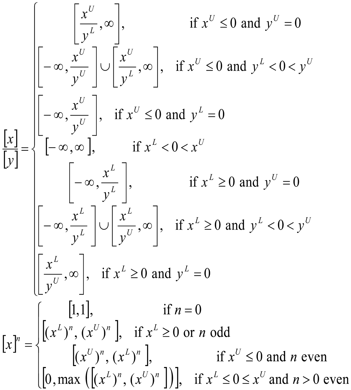
Definition 8.

The division between the interval numbers $x=[x^L,x^U]$

and $y=[y^L,y^U]$ is defined by:

${\displaystyle \frac{\left[x\right]}{\left[y\right]}}=\left[x\right]\times {\displaystyle \frac{1}{\left[y\right]}}=\left[min\left({\displaystyle \frac{x^L}{y^U}},{\displaystyle \frac{x^U}{y^L}}\right),\hspace{0.17em}max\left({\displaystyle \frac{x^L}{y^U}},{\displaystyle \frac{x^U}{y^L}}\right)\right]$ , if $0\notin \left[y\right]$.

It can be written, if$0\in \left[y\right]$ as follows:

Now we will extend the classical inequality relations between real numbers to inequality relations between interval numbers.

Let $x=\left[x^L,x^U\right]$ and $y=\left[y^L,y^U\right]$ be interval numbers, with $x^L,x^U,\hspace{0.17em}{y}^L,y^U\in R$.

Definition 9.

We say that $\left[x\right]\le \left[y\right]$ if $x^L\le y^L$ and $x^U\le y^U$.

Definition 10.

We say that $\left[x\right]<\left[y\right]$if $\left\{\begin{array}{l}{x}^L\le y^L\\ x^U<y^U\end{array}\right.$ or $\left\{\begin{array}{l}{x}^L<y^L\\ x^U\le y^U\end{array}\right.$ or $\left\{\begin{array}{l}{x}^L\le y^L\\ x^U\le y^U\end{array}\right.$.

Definition 11.

(Ishibuchi and Tanaka,1990)

We say that $\left[x\right]$≼$\left[y\right]$ if $m\left(\left[x\right]\right)\le m\left(\left[y\right]\right)$.

If $x^U\le y^L$, the interval inequality “$\left[x\right]$≼$\left[y\right]$ ” is said to be optimistic satisfactory.

If$x^U>y^L$, the interval inequality “$\left[x\right]$≼$\left[y\right]$ ”is said to be pessimistic satisfactory.

Definition 12.

We say that $\left[x\right]\prec \left[y\right]$ if $x^L\le y^U$.

Definition 13.

We say that $\left[x\right]\supset \left[y\right]$ if $x^L\le y^L$ and $x^U\ge y^U$.

2.2. Model Formulation

Notation

We consider a financial market with n risky assets for trading. Suppose that an investor intends to invest his initial wealth W₀ among the n risky assets at the beginning of period 1 for constructing a T-period investment. He can reallocate his wealth at the beginning of each of the following T-1 consecutive time periods. Since the financial market is extremely complex, many non-probabilistic factors affect the financial market. It is impossible to forecast the returns, risk and turnover rates of assets precisely by historical data. We assume that the returns, risk and turnover rates of assets are characterized by interval numbers. Let the returns of portfolios in T different periods be independent of each other. For the sake of description conveniently, let us first introduce the following notations:

${[r}_{t,i}]$ the return of risky asset i at period t, where ${[r}_{t,i}]$= [$r_{t,i}^L,r_{t,i}^U]$ , $r_{t,i}^L\le r_{t,i}^U$

${[\delta }_{i,k,t}]$ the covariance between ${[r}_{t,i}]$ and ${[r}_{t,j}]$ with ${[\delta }_{i,k,t}]$=[${\delta }_{i,k,t}^L,{\delta }_{i,k,t}^U]$,${\delta }_{i,k,t}^L\le {\delta }_{i,k,t}^U$

${ c}_{t,i}$ the transaction cost rate of risky asset i at period t;

${ x}_{t,i}$the investment proportion of risky asset i at period t;

$x_t$ the portfolio at period t, where $x_t=(x_{t,1},x_{t,2},\dots ,x_{t,n})$

$$\left[R_{P.t}\right]\mathrm{t}\mathrm{h}\mathrm{e} \mathrm{i}\mathrm{n}\mathrm{t}\mathrm{e}\mathrm{r}\mathrm{v}\mathrm{a}\mathrm{l} \mathrm{v}\mathrm{a}\mathrm{l}\mathrm{u}\mathrm{e}\mathrm{d} \mathrm{r}\mathrm{e}\mathrm{t}\mathrm{u}\mathrm{r}\mathrm{n} \mathrm{o}\mathrm{f} \mathrm{p}\mathrm{o}\mathrm{r}\mathrm{t}\mathrm{f}\mathrm{o}\mathrm{l}\mathrm{i}\mathrm{o} \mathrm{a}\mathrm{t} \mathrm{p}\mathrm{e}\mathrm{r}\mathrm{i}\mathrm{o}\mathrm{d} \mathrm{t},\left[R_{P.t}\right]=\sum _{i=1}^n{x_{t,i}[r}_{t,i}]$$

${[ R}_{N.t} ]$ the interval valued return of portfolio at period t, after paying tranxaction cost

${[ R}_t ]$the preset minimum expected interval valued return of the portfolio at period t, where ${[ R}_t ]$= [$R_t^L, R_t^U ]$, $R_t^L\le R_t^U$

${[ \delta }_t ]$ the preset maximum risk tolerance interval valued return of the portfolio at period t, where ${[ \delta }_t ]$= [${\delta }_t^L, {\delta }_t^U ]$, ${\delta }_t^L\le {\delta }_t^U$

${[I}_{t,i}]$ the interval valued turnover rate of risky asset i at period t, where ${[I}_{t,i}]$ = [$I_{t,i}^L,I_{t,i}^U]$, $I_{t,i}^L\le I_{t,i}^U$

${[ I}_t ]$ the preset minimum expected interval valued turnover rate of the portfolio at period t, where ${[ I}_t ]$= [$I_t^L, I_t^U ]$, $I_t^L\le I_t^U$

$e_t$ the preset minimum diversification degree of the t th period portfolio;

$W_t$the available wealth at the end of period t, t = 1,2,…,T.

Objective and Constraints

According to before assumptions, the returns, risk and turnover rates of risky assets are denoted as interval numbers. Then, the return and covariance of the portfolio ${ x}_t=\left({ x}_{t,1},{ x}_{t,2},\dots ,{ x}_{t,n}\right)$at period t can be, respectively, represented by

${[ R}_{P.t} ]=\sum _{i=1}^n{{ x}_{t,i} [r}_{t,i}]$ = [ $\sum _{i=1}^n{ x}_{t,i} r_{t,i }^L,\sum _{i=1}^n{ x}_{t,i}{r}_{t,i }^U$] (1)

${[ \delta }_t ]$=$\sum _{i=1}^n\sum _{k=1}^n{ { x}_{t,i }x}_{t,k}{[ \delta }_{i,k,t}]=[ \sum _{i=1}^n\sum _{k=1}^n{ { x}_{t,i }x}_{t,k}{\delta }_{i,k,t }^L,\sum _{i=1}^n\sum _{k=1}^n{ { x}_{t,i }x}_{t,k}{\delta }_{i,k,t }^U]$ (2)

For transaction cost, we use V shape function to express it. The transaction cost rate of the portfolio at period t ( t = 1, 2, …,T ) can be expressed as :

${[ C}_t ]=\sum _{i=1}^n{{ c}_{t,i} [r}_{t,i}]\left|{ x}_{t,i}-{ x}_{t-1,i} \right|$ (3), where${ c}_{t,i}$ is a crisp number for all i = 1, 2, …, n and t = 1, 2, …,T. From Eqs. (1) and (3), the return of portfolio at period t after paying transaction costs can be represented by

${ [ R}_{N.t} ]=\sum _{i=1}^n{{ x}_{t,i} [r}_{t,i}]$ - ${[ C}_t ]$ = [ $\sum _{i=1}^n{ x}_{t,i} r_{t,i }^L-C_t^U,\sum _{i=1}^n{ x}_{t,i}{r}_{t,i }^U-C_t^L$] (4)

Then, the wealth at the end of period t can be calculated by

${ W}_t=W_{0 } \prod _{j=1}^t\left( \sum _{i=1}^n{{ x}_{j,i} [r}_{j,i}]-{[ C}_j ]\right])$or

${ W_t=W}_{0 }[ \prod _{j=1}^t\left(\sum _{i=1}^n{ x}_{j,i} r_{t,i }^L-C_j^U\right), \prod _{j=1}^t\left(\sum _{i=1}^n{ x}_{j,i} r_{t,i }^U-C_j^L\right)]$ (5)

Solving Eq. (5) recursively, the terminal wealth at the end of period T is:

$W_T=W_{0 } \prod _{t=1}^T\left( \sum _{i=1}^n{{ x}_{t,i} [r}_{j,i}]-{[ C}_t ]\right])$ or

${ W}_T=W_{0 } [ \prod _{t=1}^T\left(\sum _{i=1}^n{ x}_{t,i} r_{t,i }^L-C_j^U\right), \prod _{j=1}^T\left(\sum _{t=1}^n{ x}_{j,i} r_{t,i }^U-C_j^L\right)]$ (6)

Liquidity is one of the main concerns for investors to make a portfolio decision. It measures the degree of probability of being able to transform an investment into cash without any significant loss in value. The turnover rate of an asset is the proportion of turnover volume to tradable volume of the asset, and is a factor which may reflect the asset's liquidity. Generally, investors prefer greater liquidity, especially in a bull market, returns on assets with high liquidity tend to increase with time. Here, we use the turnover rates of securities to measure their liquidity. It is known that turnover rates of assets in the future cannot be accurately predicted in a financial market. In this paper, we assume that the turnover rates of assets are characterized by interval numbers.

Based on the analysis above, the turnover rate of the portfolio at period t can be expressed by:

${[ I}_t ]=\sum _{i=1}^n{{ x}_{t,i} [I}_{t,i}]=\left[ \sum _{i=1}^n{{ x}_{t,i} I^L}_{t,i},{{ x}_{t,i} I^U}_{t,i} \right]$(7)

In the traditional portfolio theory, a distributive investment has been regarded as a good policy to reduce the risk of portfolio. Diversification degree of portfolio is also a main factor concerns for investors to make decisions. Because it is usually accepted as an instrument to diversify the unsystematic risk of portfolio. This idea is reflected in a famous saying that "one should not put all the eggs into one basket". In other words, it indicates that investors should not allocate all their money to just a few securities. Allocating all the money in only a few companies may cause financial disaster. How to obtain a well-diversified portfolio has become a problem to researchers. In this paper, we measure the diversification degree measure of portfolio at each period by using the Shannon entropy. Thus, the diversification degree of the portfolio at period t can be represented by

$H \left(x_{t }\right)=-\sum _{i=1}^n{ x}_{t,i}ln{ x}_{t,i}$, t = 1, 2, …,T (8)

The Multiperiod Portfolio Optimization Model with Interval Numbers

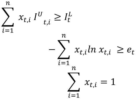
We assume that the investor is rational. He wants to maximize the terminal wealth obtained at the end of period T. At the same time, he also requires the return, risk and diversification degree of portfolio at each period that must achieve or exceed the given expected interval levels. Besides, the risk of portfolio at each period should be less than the preset maximum risk tolerance interval. Based on the analysis above, an interval multi-period portfolio selection model can be formulated as follows:

$$max{ W}_T=\max W_{0 } [ \prod _{t=1}^T\left(\sum _{i=1}^n{ x}_{t,i} r_{t,i }^L-C_j^U\right), \prod _{j=1}^T\left(\sum _{t=1}^n{ x}_{j,i} r_{t,i }^U-C_j^L\right)]$$

[ $\sum _{i=1}^n{ x}_{t,i} r_{t,i }^L-C_t^U,\sum _{i=1}^n{ x}_{t,i}{r}_{t,i }^U-C_t^L$] $\ge {[ R}_t$] (9)

$[ \sum _{i=1}^n\sum _{k=1}^n{ { x}_{t,i }x}_{t,k}{\delta }_{i,k,t }^L,\sum _{i=1}^n\sum _{k=1}^n{ { x}_{t,i }x}_{t,k}{\delta }_{i,k,t }^U]$ $\le {[ \delta }_t ] ($10)

$\left[ \sum _{i=1}^n{{ x}_{t,i} I^L}_{t,i},{{ x}_{t,i} I^U}_{t,i} \right]\ge {[ I}_t ]$(11)

$-\sum _{i=1}^n{ x}_{t,i}ln{ x}_{t,i} \ge e_t$ (12)

$$\begin{array}{l}{\sum }_{i=1}^n{ x}_{t,i}=1 \text{(13)}\\ { x}_{t,i}\ge 0 \text{i = 1,2,…,n and t = 1,2,…,T (14)}\end{array}$$

where constraint (9) means that the return of the portfolio at period t must be larger than or equal to the given minimum expected interval valued return; constraint (10) indicates that the risk of the portfolio at period t must be smaller than or equal to the preset the maximum risk tolerate interval; constraint; (11) represents that the turnover rate of the portfolio at period t must be no less than the given minimum expected interval valued level; constraint; (12) states that the diversification degree of the portfolio at period t must be no less than the given diversification level ; constraint (13) shows that the proportion at period t sums to one; constraint (14) denotes that short selling is not allowed during the whole investment.

Solution Methodology

Stage 1:Find “the best optimal solution, x⁽¹⁾” by solving the following problem: $max{W}_T=\max W_0\prod _{j=1}^T\left(\sum _{t=1}^n{x}_{j,i}{r}_{t,i}^U-C_j^L\right)$

$\sum _{i=1}^n{ x}_{t,i}{r}_{t,i }^U-C_t^L$] $\ge R_t^L$

$\sum _{i=1}^n\sum _{k=1}^n{ { x}_{t,i }x}_{t,k}{\delta }_{i,k,t }^L,]$ $\le {\delta }_{t }^U$.

$x_{t,i}\ge 0$ i = 1,2,…,n and t = 1,2,…,T

Stage 2: Find” the worst optimal solution, x⁽²⁾ “ by solving the following problem:

$$max{ W}_T=\max W_{0 } \prod _{j=1}^T\left(\sum _{t=1}^n{ x}_{j,i} r_{t,i }^L-C_j^U\right)$$

$\sum _{i=1}^n{ x}_{t,i}{r}_{t,i }^L-C_t^U$] $\ge R_t^U$

$\sum _{i=1}^n\sum _{k=1}^n{ { x}_{t,i }x}_{t,k}{\delta }_{i,k,t }^U,]$ $\le {\delta }_{t }^L$.

$\sum _{i=1}^n{{ x}_{t,i} I^L}_{t,i}\ge I_t^U$

$$\begin{array}{cc}-{\displaystyle \sum _{i=1}^n}{ x}_{t,i}ln{ x}_{t,i} \ge e_t& \\ & {\displaystyle \sum _{i=1}^n}{ x}_{t,i}=1\end{array}$$

${ x}_{t,i}\ge 0$ i = 1,2,…,n and t = 1,2,…,T

Stage 3 : We obtain the optimal solution given by: $x^0$= λx⁽¹⁾+ (1-λ)x⁽²⁾ , λ$\in$ [0,1].

2.3. Case Study: Multiperiod Portfolio Selection Under Interval Uncertainty

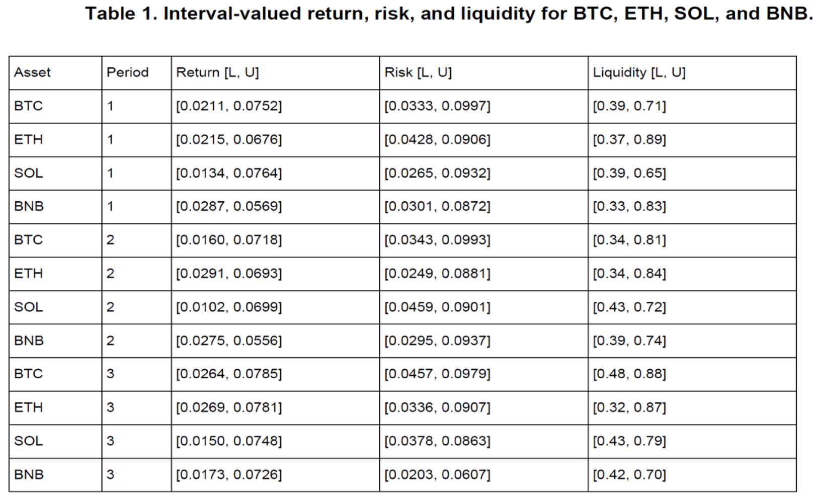
To illustrate the applicability and effectiveness of the proposed multi-period interval-based portfolio optimization model, we conduct a numerical case study using four representative assets: Bitcoin (BTC), Ethereum (ETH), Solana (SOL), and Binance Coin (BNB). The investment horizon is divided into three periods, and all input parameters, including returns, risk levels, and liquidity indicators, are modeled as intervals to reflect real-world uncertainty. The interval bounds for return and risk were derived from simulated time series reflecting historical volatility patterns and expected market dynamics, particularly tailored to the cryptocurrency domain. These intervals capture the natural uncertainty and variability inherent to high-volatility assets, enabling realistic scenario-based modeling. Table 1 presents the interval-valued returns, risk levels, and liquidity measures for each asset across the three investment periods. These values have been generated to simulate the variability and imprecision commonly observed in emerging or highly volatile markets such as cryptocurrencies.

Using the model defined in Section 2.2, we optimize the portfolio allocations under three different decision-making strategies:

-

Pessimistic: based on lower bounds for returns and upper bounds for risk.

-

Optimistic: using upper bounds for returns and lower bounds for risk.

-

Mixed: with average values between bounds, reflecting a neutral risk attitude.

The optimization objective is to maximize the interval-valued terminal wealth W_T, while satisfying constraints on return, risk, liquidity, and entropy-based diversification at each time step. For simplicity, we assume an initial wealth W₀ = 1000 u.m, a fixed transaction cost of 0.2% per asset, and a minimum diversification entropy threshold of e_t = 0.9 for all t ∈ {1,2,3}.

Optimal allocations obtained from the three strategies are summarized in Table 2.

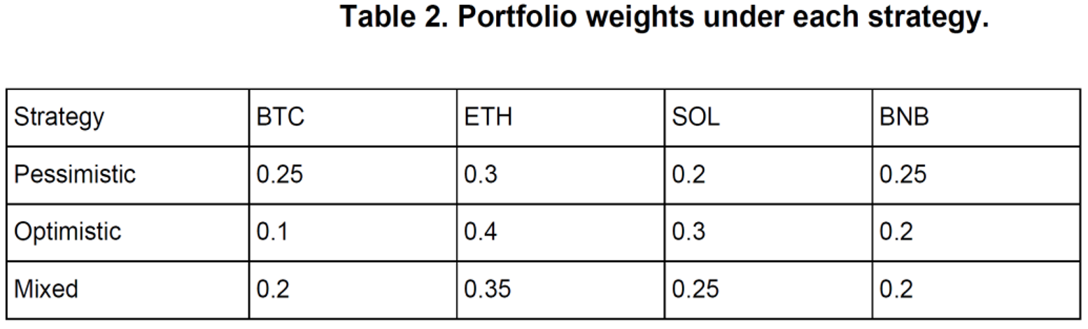
The pessimistic strategy exhibits a more conservative allocation, emphasizing assets with relatively tighter return intervals and lower downside exposure. The optimistic strategy shifts capital toward higher-return assets with broader intervals, accepting greater risk in pursuit of superior gains. The mixed strategy delivers a balanced allocation, aligning with moderate investor preferences.

The final wealth intervals W_T obtained for each strategy are as follows:

Pessimistic: [ 1085.32, 1163.77]

Mixed: [ 1123.89, 1245.16]

Optimistic: [ 1167.42, 1323.55]

These results underline the model’s ability to provide flexible solutions that adapt to different risk attitudes, while managing uncertainty in a structured way through interval analysis and entropy-based diversification.

3. Results and Discussion

In this section presents and analyzes the numerical results obtained by applying the proposed multi-period interval-based portfolio optimization model to a simulated sIn this et of assets under uncertainty. Using historical-inspired intervals for returns, risks, and liquidity of four representative cryptocurrencies (BTC, ETH, SOL, and BNB), we computed optimal portfolio allocations under three strategic scenarios: pessimistic, optimistic, and mixed.The model was solved using an initial wealth of W₀ = 1000 over three periods, withreallocation allowed at each stage. Constraints related to expected return, maximum risk, minimum liquidity, and portfolio diversification—measured via entropy—were strictly enforced at each time step.

As shown in Table 2 of Section 2.3, the portfolio allocations differ substantially across strategies. The pessimistic strategy favored a conservative distribution of capital across low-volatility assets, minimizing downside exposure. In contrast, the optimistic strategy prioritized high-return intervals, allocating more funds to riskier assets in pursuit of superior gains. The mixed strategy offered a balanced compromise, resulting in moderate allocations and diversified structure.

The resulting terminal wealth intervals, derived from cumulative returns over the three periods, are as follows:

Pessimistic:${ W}_T\in$ [ 1085.32, 1163.77]

Mixed: ${ W}_T\in$ [ 1123.89, 1245.16]

Optimistic: ${ W}_T\in$ [ 1167.42, 1323.55]

The difference between the pessimistic and optimistic outcomes highlights the sensitivity of the final wealth to investor attitude toward uncertainty. While the optimistic approach promises higher returns, it also exposes the investor to greater variability. On the other hand, the pessimistic strategy offers more stability at the cost of potential profit. The mixed approach represents a balanced trade-off, aligning with moderate risk appetite and diversified exposure. Another key insight from the results is the role of entropy-based diversification. Portfolios with higher entropy values demonstrated more even capital allocation and were less sensitive to parameter variation, especially in mixed and pessimistic scenarios. This reinforces the practical relevance of entropy as a decision-support metric in uncertain financial environments.

Overall, the case study confirms that the proposed interval-based multi-periodtimization framework offers a robust and flexible tool for portfolio selection under uncertainty. It accommodates investor preferences, reflects market imperfections, and integrates multiple performance criteria, including return, risk, liquidity, and diversification.

4. Conclusions and Future Work

The aim of this paper was to investigate the multi-period fuzzy portfolio selection problem by utilizing the concept of interval numbers derived from fuzzy set theory. To this end, we proposed a novel optimization framework that explicitly accounts for the imprecision and incompleteness of financial information, particularly relevant in emerging or volatile markets. Within the model, the return, risk, and transaction cost parameters associated with risky assets were expressed as interval-valued variables, enabling a more realistic representation of uncertainty.

The key contributions of this research can be summarized as follows. First, we formulated a multi-period fuzzy portfolio selection model that leverages interval analysis to accommodate uncertainty across multiple decision horizons. Second, we incorporated practical constraints such as transaction costs, minimum expected returns, liquidity thresholds, and diversification levels, which enhance the model’s applicability in real-world portfolio management. Third, we employed a fuzzy decision-making methodology to convert the interval-based problem into a crisp nonlinear optimization model, solvable with existing optimization tools.

To validate the model, we conducted a comprehensive case study using four representative cryptocurrencies and simulated data over a three-period horizon. The model was applied under three decision strategies—pessimistic, optimistic, and mixed—illustrating how investor attitudes toward uncertainty affect portfolio composition and terminal wealth. The results confirmed that the model is capable of generating robust solutions that balance risk, return, liquidity, and diversification objectives across multiple periods.

Future work could extend the proposed model in several directions. One potential avenue is to incorporate dynamic updating mechanisms, where interval parameters are revised at each period using real-time market data. Another interesting extension would be to explore hybrid uncertainty representations that combine interval and probabilistic components, allowing for a more nuanced treatment of risk. Additionally, heuristic or metaheuristic algorithms such as genetic algorithms, particle swarm optimization, or reinforcement learning-based methods could be employed to enhance computational efficiency, especially for large-scale portfolio problems. Finally, empirical validation using real financial datasets from various markets and asset classes could further demonstrate the practical value of the model.

References

- Alefeld G., Herzberger J. (1983). Introduction to Interval Computations. Academic Press, New York. https://www.sciencedirect.com/science/article/pii/0024379586900261.
- Allahdadi M., Nehi H.M. (2011). Fuzzy linear programming with interval linear programming approach. Advanced Modelling and Optimization, 13(1), 1–12.
- Artzner P., Delbaen F., Eber J.M., Heath D. (1999). Coherent measures of risk. Mathematical Finance, 9(3), 203–228. https://onlinelibrary.wiley.com/doi/abs/10.1111/1467-9965.00068.
- Barik S.K., Biswal M.P., Chakravartay D. (2012). Multiobjective Two-Stage Stochastic Programming Problems with Interval Discrete Random Variables. Advances in Operations Research, Article ID 279181. https://www.researchgate.net/publication/258383246_Multiobjective_Two-Stage_Stochastic_Programming_Problems_with_Interval_Discrete_Random_Variables.
- Birge J.R., Louveaux F. (1997). Introduction to Stochastic Programming. Springer, New York.
- Chinneck J.W., Ramadan K. (2000). Linear programming with interval coefficients. Journal of the Operational Research Society, 51(2), 209–220. https://www.tandfonline.com/doi/abs/10.1057/palgrave.jors.2600891.
- Fang Y., Wang S.Y. (2006). An interval semi-absolute deviation model for portfolio selection. Lecture Notes in Computer Science, 4223, 766–775. https://www.researchgate.net/publication/221086272_An_Interval_Semi-absolute_Deviation_Model_For_Portfolio_Selection.
- Follmer H., Schied A. (2004). Stochastic Finance. de Gruyter, Berlin.
- Hansen E., Walster G.W. (2004). Global Optimization Using Interval Analysis. Marcel Dekker Inc.
- Hwang C.L., Lin M. (1987). Group Decision Making under Multiple Criteria: Methods and Applications. Springer-Verlag, New York.
- Hwang C.L., Yoon K. (1981). Multiple Attribute Decision Making. Springer-Verlag, Berlin, Heidelberg, New York.
- Ishibuchi H., Tanaka H. (1990). Multiobjective programming in optimization of the interval objective function. European Journal of Operational Research, 48, 219–225. https://www.semanticscholar.org/paper/Multiobjective-programming-in-optimization-of-the-Ishibuchi-Tanaka/9582642b32be503e1bc9d39d3b2da6485fc10541.
- Jong Y. (2011). Optimization method interval portfolio selection based on satisfaction index of interval inequality relation. http://arxiv/papers/1207/1207.1932.pdf.
- Kall P., Wallace S.W. (1994). Stochastic Programming. John Wiley and Son.
- Kambo N.S. (1997). Mathematical Programming Techniques. Affiliated East-West Press, New York.
- Markowitz H. (1952). Portfolio selection. Journal of Finance, 7, 77–91.
- Moore R.E. (1966). Interval Analysis. Prentice-Hall, Englewood Cliffs, NJ.
- Moore R.E. (1979). Methods and Application of Interval Analysis. SIAM, Philadelphia.
- Nobibon F.T., Guo R. (2006). Foundation and formulation of stochastic interval programming. PGD Thesis, African Institute for Mathematical Sciences, Cape Town, South Africa.
- Ogryczak W. (2002). Multiple criteria optimization and decisions under risk. Control and Cybernetics, 31(4), 975–1003. https://www.researchgate.net/publication/269027165_Multiple_criteria_optimization_and_decisions_under_risk.
- Ruszczynski A., Shapiro A. (2003). Stochastic Programming. Elsevier, Vol. 10.
- Sayin S., Kouvelis P. (2005). The multiobjective discrete optimization problem: A weighted min-max two-stage optimization approach and a bicriteria algorithm. Management Science, 51(10), 1572–1581.
- Şerban, F.; Ştefănescu, M.V; Dedu, S( 2011)The Relationship Profitability–Risk for an Optimal Portfolio Building with Two Risky Assets and a Risk-Free Asset. Int. J. Med. Eng. Inform., 5, 299–306. https://www.researchgate.net/publication/255992745_The_Relationship_Profitability_-_Risk_for_an_Optimal_Portfolio_Building_with_Two_Risky_Assets_and_a_Risk-Free_Asset.
- Sheraz, M., Dedu, S., & Preda, V. (2022). Volatility dynamics of non-linear volatile time series and analysis of information flow: Evidence from cryptocurrency data. Entropy, 24(10), 1410. https://pmc.ncbi.nlm.nih.gov/articles/PMC9601717/.
- Shapiro A., Dentcheva D., Ruszczynski A. (2009). Lectures on Stochastic Programming: Modeling and Theory. MOS-SIAM Series on Optimization, Vol. 9, 1–436. https://epubs.siam.org/doi/book/10.1137/1.9781611976595.
- Toma A., Dedu S. (2014). Quantitative techniques for financial risk assessment: a comparative approach using different risk measures and estimation methods. Procedia Economics and Finance, 8, 712–719.https://www.researchgate.net/publication/275245470_Quantitative_Techniques_for_Financial_Risk_Assessment_A_Comparative_Approach_Using_Different_Risk_Measures_and_Estimation_Methods.
Disclaimer/Publisher’s Note: The statements, opinions and data contained in all publications are solely those of the individual author(s) and contributor(s) and not of MDPI and/or the editor(s). MDPI and/or the editor(s) disclaim responsibility for any injury to people or property resulting from any ideas, methods, instructions or products referred to in the content. |
© 2025 by the author. Licensee MDPI, Basel, Switzerland. This article is an open access article distributed under the terms and conditions of the Creative Commons Attribution (CC BY) license (http://creativecommons.org/licenses/by/4.0/).
Copyright: This open access article is published under a Creative Commons CC BY 4.0 license, which permit the free download, distribution, and reuse, provided that the author and preprint are cited in any reuse.