A Multi-objective Optimization Framework for Portfolio Selection

1. Introduction

Portfolio selection theory originates from the seminal work of Markowitz [15], in which return is quantified as the mean and risk as the variance. In most of the existing portfolio selection models, return and risk are considered the two fundamental factors that guide investors' choices. However, it is often observed that not all relevant information for portfolio selection can be captured by these two metrics alone. Other considerations, such as liquidity, transaction costs, and uncertainty, may be equally or even more important for investors [2,3,5]. Including these additional criteria in the portfolio selection process may lead to more balanced and satisfactory investment decisions, especially when the sacrifice in return or risk is compensated by superior performance under other criteria [4,6]. As a result, multicriteria portfolio selection models have attracted considerable attention in the literature [5,7,11]. These models enable the simultaneous consideration of multiple objectives, thereby reflecting more accurately the complex preferences of real-world investors. In practice, investors often rebalance their portfolios over time by buying or selling assets in response to market dynamics. This process incurs transaction costs, which are a significant concern for portfolio managers aiming to build efficient and realistic investment models [13,14,26]. While some studies consider fixed transaction costs [4,18], more recent approaches introduce nonlinear or incremental cost functions that better reflect real trading conditions [8,21]. Since the introduction of the mean–variance model [15], variance has remained the most commonly used risk measure. However, it has notable limitations—particularly its inability to distinguish between downside risk (losses) and upside potential (gains). For this reason, downside risk measures such as semi-variance [22,23] and semi-absolute deviation [24] have been proposed as more appropriate alternatives, especially when investors are primarily concerned about portfolio underperformance. Semi-variance, initially introduced by Markowitz [22], only penalizes deviations below a target return. While more intuitive than variance, its implementation is computationally intensive due to its nonlinear nature [23,24,25]. In contrast, the semi-absolute deviation measure, proposed by Sprenza [24], shares the same focus on downside risk but enables a linear programming formulation, which is far more efficient to solve, especially for portfolios involving a large number of assets [8].

Another critical issue in portfolio optimization is uncertainty. In real-world scenarios, decision-makers rarely possess exact or complete information regarding input parameters such as expected returns, variances, or correlations. This uncertainty can arise from different sources and may be interpreted as either randomness or fuzziness [1,13,20]. Stochastic programming has been widely used to address randomness [5,20], whereas fuzzy programming handles fuzziness through membership functions [2,13]. However, both approaches require detailed assumptions about probability distributions or fuzzy sets, which are difficult to estimate accurately in practice [25]. As an alternative, interval programming assumes that only the bounds (lower and upper limits) of uncertain parameters are known. This method has the advantage of not requiring probabilistic distributions or fuzzy logic membership functions, making it more flexible and easier to implement [16,17,19]. Interval programming has been successfully applied in portfolio selection models [6,10,12], particularly in cases where market data is scarce, imprecise, or volatile.

This paper proposes a new multi-objective portfolio rebalancing framework that incorporates interval representations of return, semi-absolute deviation as a risk measure, and nonlinear transaction costs. The aim is to construct robust portfolios that respond realistically to uncertainty and market friction, while capturing multiple investor objectives

2. Materials and Methods

2.1. Interval Analysis Background

Many relations and operations defined on sets or pairs of real numbers can be extended to operations on intervals. Let $x=\left[x^L,x^U\right]$and $y=\left[y^L,y^U\right]$be interval  numbers as formalized in [17,18] and widely used in applications under uncertainty.”.   Interval numbers are used to represent imprecise data, where only the lower and upper bounds are available [1,12].

Definition 1. 

The equality between interval numbers is defined as follows:

$$\left[x\right]=\left[y\right]\mathrm{if}{x}^L=y^L\mathrm{and}{x}^U=y^U.$$

Definition 2. 

The median of the interval number $x=\left[x^L,x^U\right]$is defined by:

$$m\left(x\right)={\displaystyle \frac{x^L+x^U}{2}}.$$

Definition 3. 

The product between the real number a and the interval number $\left[x\right]$ is defined by:

$$a\cdot \left[x\right]=\left\{a\cdot x|x\in \left[x\right]\right\}=\left\{\begin{array}{c}\left[a\cdot x^L,a\cdot x^U\right],ifa>0\\ \left[a\cdot x^U,a\cdot x^L\right],ifa<0\\ \left[0\right],ifa=0\end{array}\right..$$

Let $x=\left[x^L,x^U\right]$ and $y=\left[y^L,y^U\right]$ be interval numbers.

Definition 4. 

The summation between two interval numbers is defined by:

$$\left[x\right]+\left[y\right]=\left[x^L+y^L,x^U+y^U\right].$$

Definition 5. 

The subtraction between two interval numbers is defined as follows:

$$\left[x\right]-\left[y\right]=\left[x^L-y^U,x^U-y^L\right].$$

Definition 6. 

The product between two interval numbers is defined by:

$$\left[x\right]\times \left[y\right]=\left[min\left(x^L{y}^L,x^L{y}^U,x^U{y}^L,x^U{y}^U\right),max\left(x^L{y}^L,x^L{y}^U,x^U{y}^L,x^U{y}^U\right)\right].$$

Definition 7. 

The inverse of the interval number $y=\left[y^L,y^U\right]$ is defined by:

$${\displaystyle \frac{1}{\left[y\right]}}=\left[{\displaystyle \frac{1}{y^U}},{\displaystyle \frac{1}{y^L}}\right]\mathrm{if}0\notin \left[y\right].$$

Definition 8. 

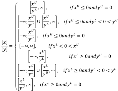
The division between the interval numbers $x=\left[x^L,x^U\right]$ and $y=\left[y^L,y^U\right]$is defined by:

$${\displaystyle \frac{\left[x\right]}{\left[y\right]}}=\left[x\right]\times {\displaystyle \frac{1}{\left[y\right]}}=\left[min\left({\displaystyle \frac{x^L}{y^U}},{\displaystyle \frac{x^U}{y^L}}\right),max\left({\displaystyle \frac{x^L}{y^U}},{\displaystyle \frac{x^U}{y^L}}\right)\right]\mathrm{if}0\notin \left[y\right].$$

It can be written, if$0\in \left[y\right]$ as follows:

$${\left[x\right]}^n=\left\{\begin{array}{c}\begin{array}{cc}\left[1,1\right],& ifn=0\\ \left[{(x^L)}^n,{(x^U)}^n\right],& if{x}^L\ge 0ornodd\end{array}\\ \begin{array}{cc}\left[{(x^U)}^n,{(x^L)}^n\right],& if{x}^U\le 0andneven\\ \left[0,max\left(\left[{(x^L)}^n,{(x^U)}^n\right]\right)\right],& if{x}^L\le 0\le x^{U}andn>0even\end{array}\end{array}\right.$$

Now we will extend the classical inequality relations between real numbers to inequality relations between interval numbers.

Let $x=\left[x^L,x^U\right]$ and $y=\left[y^L,y^U\right]$ be interval numbers, with $x^L,x^U,y^L,y^U\in R$.

Definition 9. 

We say that $\left[x\right]\le \left[y\right]$ if  $x^L\le y^L$ and $x^U\le y^U$.

Definition 10. 

We say that $\left[x\right]<\left[y\right]$ if  $\left\{\begin{array}{c}{x}^L\le y^L\\ x^U<y^U\end{array}\right.$ or $\left\{\begin{array}{c}{x}^L<y^L\\ x^U\le y^U\end{array}\right.$ or  $\left\{\begin{array}{c}{x}^L\le y^L\\ x^U\le y^U\end{array}\right.$.

Definition 11. 

(Ishibuchi and Tanaka,1990)

We say that $\left[x\right]$≼$\left[y\right]$if $m\left(\left[x\right]\right)\le m\left(\left[y\right]\right)$.

If $x^U\le y^L$, the interval inequality  “$\left[x\right]$≼$\left[y\right]$” is said to be optimistic satisfactory.

If$x^U>y^L$,  the interval inequality  “$\left[x\right]$≼$\left[y\right]$” is said to be pessimistic satisfactory.

Definition 12. 

We say that $\left[x\right]\prec \left[y\right]$

if $x^L\le y^U$.

Definition 13. 

We say that $\left[x\right]\supset \left[y\right]$

if $x^L\le y^L$and $x^U\ge y^U$.

2.2. Model Formulation

Notation

The general multi-objective modeling framework is adapted from Guu et al. (2014), who proposed a supplier portfolio optimization model using interval coefficients and multiple decision-making strategies. In this paper, we extend their structure to financial assets, reformulating the objectives as return, risk, and liquidity, and applying them in the context of cryptocurrency portfolios. For completeness and consistency, we follow the notation and conventions established in their work, while applying them to a novel context and asset class here

In this section, for portfolio optimization, we use the semiabsolut mean deviation, where the future income assets are treated as interval numbers.

Suppose an investor wants to allocate some capital in n risky assets. We introduce the following notations as applied in multiobjective decision environments [6,12].

$T$the time horizon of the investment;

$r_i$the average return of the i-th asset;

$r_{it}$the historical return of the i-th asset over the period t, with i=$\overline{1,n}$, t ∈$\overline{1,T}$;

$r_{ai}$the average return of the asset i on the time horizon T, i=$\overline{1,n}$; where:

$x_i^0$the initial proportion of total funds invested in the i-th asset, before rebalancing;

$x_i$the final proportion of total funds invested in the i-th asset, after rebalancing;

C ($x_i$) the transaction cost incurred on buying or selling proportion of the i-th asset , i = $\overline{1,n+1.}$$C\left(x\right)$ the total transaction cost proportion of portfolio rebalancing:

Objective, constraints and the decision model

Net return

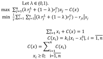
The maximization form of the net return of the portfolio after adjusting transaction cost is expressed as:

$$\max f_1(x)={{\displaystyle \sum }}_{j=1}^n\left[r_j\right]x_j-C\left(x\right)=\left[{{\displaystyle \sum }}_{j=1}^n{r}_j^L{x}_j-C\left(x\right),{{\displaystyle \sum }}_{j=1}^n{r}_j^U{x}_j-C\left(x\right)\right].$$

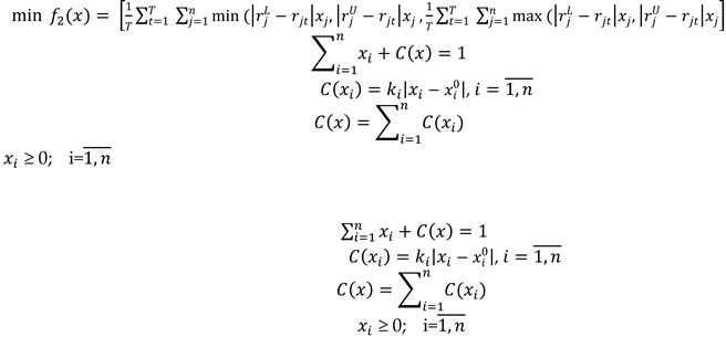
Risk

Risk is an important issue while modelling portfolio selection problem. In this paper, portfolio risk is quantified using the deviation of return expected return of the portfolio [14,26]

The average rate of return of the asset j, j=$\overline{1,n}$, can be represented using the following interval numbers: $\left[r_j\right]=\left[r_j^L,r_j^U\right]=\left[min\left\{r_{aj},r_{hj}\right\},max\left\{r_{aj},r_{hj}\right\}\right]$,where:

$-r_{aj}$is the arithmetic mean of the asset returns j, j=1,n (average yield) based on historical data, expressed as:$r_{aj}$=${\displaystyle \frac{1}{T}}{\displaystyle \sum }_{t=1}^T{r}_{jt}$$-r_{hj}$is the historical mean return tendency of asset returns j, j=1,n; (if asset j yields have been increasing, it is acceptable that the yield is higher arithmetic performance based on historical data)

Then the average rate of return of the portfolio $x$is given by:

$$\left[r\left(x\right)\right]={{\displaystyle \sum }}_{j=1}^n[r_j]x_j=\left[{{\displaystyle \sum }}_{j=1}^n{r}_j^L{x}_j,{{\displaystyle \sum }}_{j=1}^n{r}_j^U{x}_j\right]$$

Since the average yields of assets are modeled using interval numbers, we can quantify the deviation of the portfolio return We will use a interval number:

$$\left[{\omega }_t\left(x\right)\right]=\left[{\omega }_t{\left(x\right)}^L,{\omega }_t{\left(x\right)}^U\right]=\left[\min {{\displaystyle \sum }}_{j=1}^n(\left|r_j^L-r_{jt}\right|x_j,\left|r_j^U-r_{jt}\right|x_j,\max {\displaystyle \sum }_{j=1}^n(\left|r_j^L-r_{jt}\right|x_j,\left|r_j^U-r_{jt}\right|x_j\right].$$

Then the mean semi-absolute deviation interval for the portfolio x is:

$\left[\omega \left(x\right)\right]={\displaystyle \frac{1}{T}}{\displaystyle \sum }_{t=1}^T\left[{\omega }_t\left(x\right)\right].$. We will use $\left[\omega \left(x\right)\right]$to assess the risk of the portfolio x.

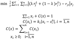
The minimization form of the portfolio risk is thus expressed as :$\min f_2(x)=$

$$\left[{\displaystyle \frac{1}{T}}{\displaystyle \sum }_{t=1}^T{\displaystyle \sum }_{j=1}^n\min (\left|r_j^L-r_{jt}\right|x_j,\left|r_j^U-r_{jt}\right|x_j,{\displaystyle \frac{1}{T}}{\displaystyle \sum }_{t=1}^T{\displaystyle \sum }_{j=1}^n\max (\left|r_j^L-r_{jt}\right|x_j,\left|r_j^U-r_{jt}\right|x_j\right].$$

Constraints

Capital budget constraint: Assuming that the investor does not invest any additional capital during portfolio rebalancing, the following constraint must hold:

$${{\displaystyle \sum }}_{i=1}^n{x}_i+C\left(x\right)=1,$$

Cost constraints: the following constraints must hold:

$$C\left(x_i\right)=k_i\left|x_i-x_i^0\right|;$$

$$C\left(x\right)={{\displaystyle \sum }}_{i=1}^n{x}_i;i=\overline{1,n}$$

No short selling of assets is expressed as:$x_i$≥ 0;  i=$\overline{1,n}$The decision model (_P1)

The multiobjective portfolio rebalancing model is formulated as follows:

$$\max f_1(x)=\left[{{\displaystyle \sum }}_{j=1}^n{r}_j^L{x}_j-C\left(x\right),{{\displaystyle \sum }}_{j=1}^n{r}_j^U{x}_j-C\left(x\right)\right]$$

Solution methodology

For determining an optimal solution of the problem (P1) we can use the strategies:

The pessimistic strategy (P₂)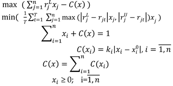

The optimistic strategy (P₃)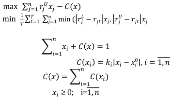

The mixt strategy(P₄)

2.3. Case Studies

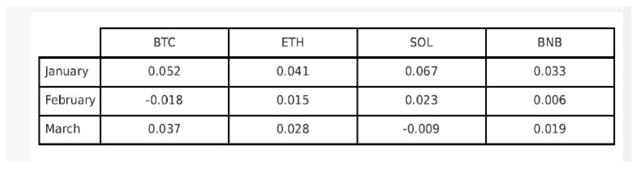
To illustrate the practical applicability of the proposed multiobjective optimization framework, we consider a simulated portfolio rebalancing problem involving four popular cryptocurrencies: Bitcoin (BTC), Ethereum (ETH), Solana (SOL), and Binance Coin (BNB). The investment horizon is three months, covering the period from January to March 2025, with monthly rebalancing..which have been shown to exhibit nonlinear and high volatility [25]. The goal is to construct an optimal portfolio that maximizes net return and minimizes risk (defined via semi-absolute deviation), under transaction costs and interval uncertainty of returns. following approaches similar to [18] for uncertain data . We assume that historical returns for each asset over the three-month period are known and summarized in the matrix below. The values represent the realized returns for each asset in each month:

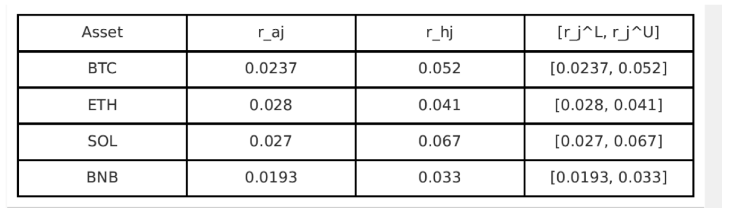
Based on these data, we compute the arithmetic mean ( $r_{aj})$​ and the historical trend ​value $(r_{hj}-$ defined as the highest return within the period). The interval representation of expected returns for each asset is then defined as:

$\left[r_j\right]=\left[r_j^L,r_j^U\right]=\left[min\left\{r_{aj},r_{hj}\right\},max\left\{r_{aj},r_{hj}\right\}\right]$

To determine the optimal portfolio allocations under each decision-making strategy, we conducted a numerical simulation using MATLAB. The simulation follows a modular computational pipeline combining interval arithmetic, entropy-based diversification metrics, and nonlinear constrained optimization. This setup enables a structured and realistic implementation of the theoretical model. We consider an initial allocation vector $x_0$ = (0.25, 0.25, 0.25,0.25), and assume that the investor wishes to rebalance the portfolio under transaction cost coefficients $ki$= 0. 01 for each asset. The constraints defined in Section 2.2 are fully imposed: total capital conservation, no short selling, and proportional transaction cost. To analyze the robustness of the proposed model, we solve 3 scenarios.

Pessimistic Scenario (Model P₂)

This model considers the lower bound of returns and the upper bound of risk, reflecting a conservative investor's attitude. The objective is:

$$\max ({{\displaystyle \sum }}_{j=1}^n{r}_j^L{x}_j-C\left(x\right));$$

The optimal allocation: $x_{pesimist}^{*}$= (0.28, 0.22, 0.25, 0.25)

Net return interval: [0.0304, 0.0489]

Risk interval: [0.011, 0.023]

Optimistic Scenario (Model P₃)

This model considers the upper bound of returns and the lower bound of risk, reflecting a conservative investor's attitude. The objective is:

$$\begin{gathered} \max {{\displaystyle \sum }}_{j=1}^n{r}_j^U{x}_j-C\left(x\right)\min {\displaystyle \frac{1}{T}}{\displaystyle \sum }_{t=1}^T{\displaystyle \sum }_{j=1}^n\min (\left|r_j^L-r_{jt}\right|x_j,\left|r_j^U-r_{jt}\right|x_j \\ {{\displaystyle \sum }}_{i=1}^n{x}_i+C\left(x\right)=1C\left(x_i\right)=k_i\left|x_i-x_i^0\right|,i=\overline{1,n}C\left(x\right)={{\displaystyle \sum }}_{i=1}^{n}C(x_i)x_i\ge 0;\mathrm{i}=\overline{1,n} \end{gathered}$$

The optimal allocation: $x_{optimist}^{*}$= (0.20, 0.30, 0.30, 0.20)

Net return interval: [0.0341, 0.0544]

Risk interval: [0.07, 0.017].

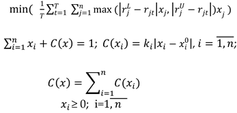
The mixt strategy (Model P₄)

Here, we consider a balanced strategy by averaging the upper and lower interval endpoints with λ = 0.5, reflecting a neutral investor perspective

$$\max {{\displaystyle \sum }}_{j=1}^n\left((\mathsf{\lambda }{r}_j^L+\left(1-\mathsf{\lambda }\right)r_j^U\right)x_j-C\left(x\right))$$

The optimal allocation: $x_{mixt}^{*}$= ( 0.26, 0.26, 0.24, 0.24 )

Net return interval: [0.0322, 0.0512]

Risk interval: [0.09, 0.020]

These case studies confirm the adaptability of the proposed framework under various investor attitudes and market expectations. The use of interval numbers and semi-absolute deviation allows a nuanced view of risk under uncertainty, while the flexible multiobjective structure enables tailored optimization depending on investor preference

3. Results and Discussions

This section presents and interprets the numerical results obtained from the case study described in Section 2.3. Using the simulated data for four major cryptocurrencies—Bitcoin, Ethereum, Solana, and Binance Coin—across a three-month investment horizon, we applied the proposed multiobjective optimization framework under three distinct investor strategies: pessimistic, optimistic, and mixed.

Each strategy was evaluated using the interval-based formulations for expected returns and semi-absolute deviation as a risk measure. Transaction costs were incorporated explicitly in the model, using a proportional cost function. The decision models were solved using predefined weight coefficients w₁​=0.6 and w_2​=0.4, reflecting a moderate preference for return over risk minimization.

3.1. Portfolio Allocations

The optimal portfolio allocations obtained under each strategy are summarized below:

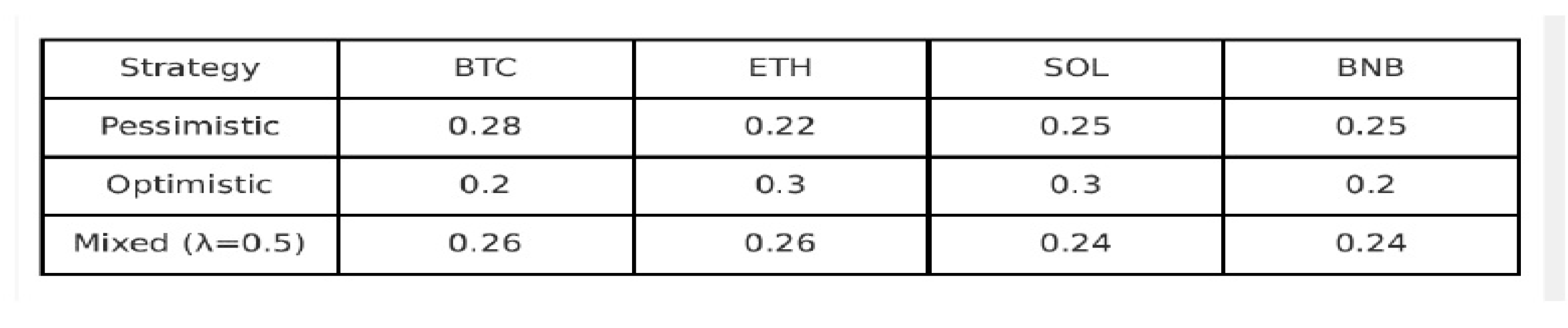
These results show that the pessimistic strategy favors safer assets (e.g., BTC) with more conservative return intervals, while the optimistic strategy tilts toward riskier but potentially more rewarding assets like SOL and ETH. The mixed strategy offers a balanced diversification across all assets, providing stability without sacrificing expected returns

3.2. Net Return and Risk Intervals

The performance of each strategy was assessed in terms of net return and risk, both modeled as interval values:

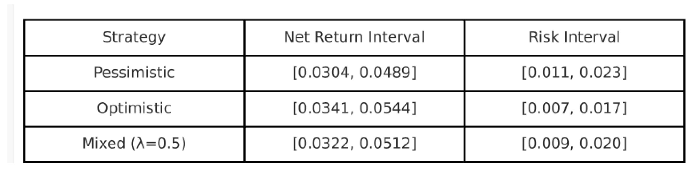
It is evident that the optimistic strategy yields the highest potential return, but at the cost of lower robustness under adverse scenarios. Conversely, the pessimistic model provides the lowest expected return, but it is the most conservative in terms of risk exposure.The mixed strategy demonstrates that a trade-off is possible, achieving a relatively high return with moderate risk. The use of the parameter λ for controlled interpolation between the extremes of optimism and pessimism.

3.3. Strategic Insights

Several insights can be drawn from these findings:

-Interval analysis provides a more nuanced understanding of performance, especially under conditions of uncertainty. Instead of fixed expectations, investors gain a spectrum of possible outcomes.

-The multiobjective approach ensures that no single objective dominates the decision-making process. Instead, trade-offs between return and risk are explicitly modeled.

-Transaction costs play a critical role in determining final allocations, especially in high-frequency rebalancing scenarios. Ignoring them would lead to unrealistic investment strategies.

-The choice of strategy depends largely on the investor's risk appetite. The pessimistic strategy is suitable for risk-averse individuals, while the optimistic strategy appeals to aggressive investors seeking higher returns.

4. Conclusions and Future Work

This paper proposed a multiobjective portfolio rebalancing model that incorporates nonlinear transaction costs and interval-based uncertainty. The model reflects realistic market conditions by assuming that the investor pays variable transaction fees depending on the proportion of each asset bought or sold, based on incremental discount schemes. The optimization process aims to determine an adjusted portfolio allocation that balances three key financial objectives: maximizing return, minimizing risk, and maintaining liquidity. By modeling expected returns as interval numbers and quantifying risk through the semi-absolute deviation of returns, the proposed framework provides a robust decision-making tool under uncertainty. The formulation includes constraints related to capital conservation, no short selling, and proportional transaction costs, ensuring its practical applicability. Numerical simulations based on a portfolio of four cryptocurrencies over a three-month horizon demonstrate how different investor attitudes—pessimistic, optimistic, or mixed—can influence the optimal asset allocation and the resulting return-risk trade-off.

The results highlight that interval analysis enhances the investor’s understanding of possible outcomes and provides more informative insights than point-estimate models. Furthermore, the multiobjective structure of the optimization problem allows for strategic flexibility and can be tailored to various levels of risk aversion.

Future research may extend this model in several directions. One potential avenue involves the inclusion of real-time market dynamics, such as high-frequency trading signals or regime-switching behaviors. Another direction is to incorporate machine learning techniques for interval estimation and portfolio risk forecasting. In addition, testing the model using empirical data from traditional financial markets or integrating alternative asset classes such as NFTs or tokenized securities could further validate and broaden the applicability of the proposed framework

References

- Alefeld, G.; Herzberger, J. (1983). Introduction to Interval Computations. Academic Press, New York. https://www.sciencedirect. 0024. [Google Scholar]
- Allahdadi, M.; Nehi, H.M. Fuzzy linear programming with interval linear programming approach. Advanced Modelling and Optimization 2011, 13, 1–12. [Google Scholar]
- Artzner, P.; Delbaen, F.; Eber, J.M.; Heath, D. Coherent measures of risk. Mathematical Finance 1999, 9, 203–228. [Google Scholar] [CrossRef]
- Barik, S.K.; Biswal, M.P.; Chakravartay, D. Multiobjective Two-Stage Stochastic Programming Problems with Interval Discrete Random Variables. Advances in Operations Research, 2012, 279181. https://www.researchgate. 2583. [Google Scholar]
- Birge, J.R.; Louveaux, F. (1997). Introduction to Stochastic Programming. Springer, New York.
- Chinneck, J.W.; Ramadan, K. Linear programming with interval coefficients. Journal of the Operational Research Society 2000, 51, 209–220. [Google Scholar] [CrossRef]
- Fang, Y.; Wang, S.Y. An interval semi-absolute deviation model for portfolio selection. Lecture Notes in Computer Science 2006, 4223, 766–775. [Google Scholar]
- Guu, S.-M.; Mehlawat, M.; Kumar, S. A Multiobjective Optimization Framework for Optimal Selection of Supplier Portfolio. Optimization, 2014, 63, 1491–1512. [Google Scholar] [CrossRef]
- Hwang, C.L.; Lin, M. (1987). Group Decision Making under Multiple Criteria: Methods and Applications. Springer-Verlag, New York.
- Hwang, C.L.; Yoon, K. (1981). Multiple Attribute Decision Making. Springer-Verlag, Berlin, Heidelberg, New York.
- Ishibuchi, H.; Tanaka, H. Multiobjective programming in optimization of the interval objective function. European Journal of Operational Research 1990, 48, 219–225. [Google Scholar] [CrossRef]
- Jong, Y. (2011). Optimization method interval portfolio selection based on satisfaction index of interval inequality relation. http://arxiv/papers/1207/1207.1932.
- Kall, P.; Wallace, S.W. (1994). Stochastic Programming. John Wiley and Sons.
- Kambo, N.S. (1997). Mathematical Programming Techniques. Affiliated East-West Press, New York.
- Markowitz, H. Portfolio selection. Journal of Finance 1952, 7, 77–91. [Google Scholar]
- Moore, R.E. Interval Analysis. Prentice-Hall, Englewood Cliffs, NJ, 1966.
- Moore, R.E. Methods and Application of Interval Analysis. SIAM, Philadelphia, 1979.
- Nobibon, F.T.; Guo, R. Foundation and formulation of stochastic interval programming. PGD Thesis, African Institute for Mathematical Sciences, Cape Town, South Africa, 2006. [Google Scholar]
- Ogryczak, W. Multiple criteria optimization and decisions under risk. Control and Cybernetics 2002, 31(4), 975–1003. https://www.researchgate. 2690. [Google Scholar]
- Ruszczynski, A.; Shapiro, A. (2003). Stochastic Programming. Elsevier, Vol. 10.
- Sayin, S.; Kouvelis, P. The multiobjective discrete optimization problem: A weighted min-max two-stage optimization approach and a bicriteria algorithm. Management Science 2005, 51, 1572–1581. [Google Scholar] [CrossRef]
- Şerban, F.; Ştefănescu, M.V.; Dedu, S. The Relationship Profitability–Risk for an Optimal Portfolio Building with Two Risky Assets and a Risk-Free Asset. Int. J. Med. Eng. Inform. 2011, 5, 299–306. [Google Scholar]
- Sheraz, M.; Dedu, S.; Preda, V. Volatility dynamics of non-linear volatile time series and analysis of information flow: Evidence from cryptocurrency data. Entropy 2022, 24, 1410. [Google Scholar] [CrossRef] [PubMed]
- Shapiro, A.; Dentcheva, D.; Ruszczynski, A. Lectures on Stochastic Programming: Modeling and Theory. MOS-SIAM Series on Optimization 2009, 9, 1–436. [Google Scholar]
- Toma, A.; Dedu, S. Quantitative techniques for financial risk assessment: a comparative approach using different risk measures and estimation methods. Procedia Economics and Finance 2014, 8, 712–719. [Google Scholar] [CrossRef]
Figure 2.
Expected returns for each asset.
Figure 4.
The performance of each strategy.
Disclaimer/Publisher’s Note: The statements, opinions and data contained in all publications are solely those of the individual author(s) and contributor(s) and not of MDPI and/or the editor(s). MDPI and/or the editor(s) disclaim responsibility for any injury to people or property resulting from any ideas, methods, instructions or products referred to in the content. |
© 2025 by the authors. Licensee MDPI, Basel, Switzerland. This article is an open access article distributed under the terms and conditions of the Creative Commons Attribution (CC BY) license (http://creativecommons.org/licenses/by/4.0/).
Copyright: This open access article is published under a Creative Commons CC BY 4.0 license, which permit the free download, distribution, and reuse, provided that the author and preprint are cited in any reuse.