
Submitted:
10 April 2025
Posted:
11 April 2025
You are already at the latest version
Abstract
Thanks to Light Detection and Ranging (LiDAR), autonomous vehicles are able to detect different objects in their environment and measure the distance between them. This device gives an un-manned ground vehicle the ability to see its surroundings in real time. However, the accuracy of LiDAR can be reduced, especially in rainy weather, fog, urban smog and the like. These factors can have disastrous consequences as it increases errors in the vehicle's control computer. The aim of this research was to determine the most appropriate LiDAR frequency for autonomous vehicles, depending on the distance to them and scanning frequency in various weather conditions, therefore it is based on empiric data obtained by using the RoboPeak A1M8 LiDAR. The results obtained in rainy conditions are compared with the same ones in clear weather, using stochastic methods. A direct influence of both the frequencies used and the rain on the accuracy of the LiDAR measurements was found. Range measurement errors increase in rainy weather; as the scanning frequency increases, the results become more accurate but capture a smaller number of object points. The higher frequencies lead to about five times less error at the farthest distances compared to the lower frequencies.
Keywords:
autonomous vehicle
; RoboPeak A1M8 laser scanner
; LiDAR
; distance
; stochastic methods
1. Introduction
Autonomous vehicles are one of the most rapidly developing areas of transport, where the latest technologies and achievements in sensors, artificial intelligence and information technologies are concentrated [1,2,3]. It is expected that the latest technologies in this field and the development of new driving functions will have a positive impact on the economic, natural and social environment [4,5,6,7], according to the work of large scientific teams, experienced engineers as well as students and even junior researchers.
The system of autonomous vehicles needs to detect various objects in the environment and at the same time evaluate distances, usually using a laser range finder (hereafter referred to as LiDAR) [8,9]. This device is considered one of the most important because it gives an unmanned ground vehicle the ability to see its surroundings in real time.
The accuracy of modern LiDAR distance measurements is relatively low. Ongoing work in this area will correct this drawback and, according to the authors of the paper [10,11,12], this improvement in LiDAR will allow it to be used in even more applications.
There are 6 factors that generally affect the return signal and adversely affect the results, and they can be divided into the following groups: false detection of various objects (cars, pedestrians or other infrastructure), noise in the optical unit or detector amplifier, electromagnetic interference, too high signal level in the receiver circuit, ground relief reflections and false detections in changing weather conditions [13,14]. Additional factors (such as driving parameters and the type of surface being scanned) also affect the accuracy of LiDAR readings.
To date, there has been little research evaluating the accuracy of LiDAR performance in autonomous vehicles. Most of it focuses on LiDAR applications for unmanned aerial vehicles (UAVs). However, some conclusions on LiDAR accuracy can be drawn from the analysis of such studies.
For example, [15,16,17,18] states that LiDAR research data cannot replace traditional distance measurements when centimeter or even millimeter accuracy is required. Similarly, [19] found that the accuracy of a LiDAR mounted on a UAV reached 10 cm or more when the LiDAR was 50 m away from the object.
Various LiDAR result processing algorithms [20], such as iterative closed point (ICP) algorithms, generalized ICP algorithms and normal distributions transform (NDT) algorithms, have been proposed to improve measurement accuracy [13,21,22,23]. However, the use of such algorithms requires a large number of points, which is not always available.
One of the few studies on the accuracy of LiDAR in cars is presented in [24], where the Pro-SiVIC LiDAR was investigated by simulating normal weather conditions and using a laser beam with the following parameters: wavelength λ = 905 nm, pulse energy 1.6 μJ, pulse duration 16 ns, divergence 0.07°. The results obtained show how the signal-to-noise ratio (SNR) changes as a function of the distance between the sensor and the car. It can be seen that the SNR values are higher when the signal is reflected by the car body. This is due to the nature of the metal material, which can reflect more than plastic or semi-transparent objects such as glass. Signal intensity decreases with distance according to Lambert's law of light absorption. The LiDAR receiver can also detect the return signal from objects with strong reflective properties (e.g., metal surfaces) at long range (190 m). The detection range can be extended by increasing the laser power or reducing the beam divergence.
In summary, reflective objects with flat metal surfaces such as trucks, cars and road signs can be detected at a distance of more than 100 meters under normal weather conditions: For motorcycles and pedestrians, the maximum detection distance is lower because there are fewer or no metal surfaces. The signal decays exponentially as the distance between the LiDAR and the vehicle increases. With a dense distribution of water particles in the atmosphere (rain, fog), the signal amplitude decreases rapidly, and the range of detectable distance decreases many times. As a result, it can be difficult to maintain a safe distance between vehicles in poor visibility [25], and it would be difficult to control the situation if, for example, an oncoming vehicle suddenly brakes [10,15,19,21,22,24].
Thus, the purpose of this research is to determine the most appropriate LiDAR frequency for autonomous vehicles, depending on the distance to them, as well as evaluating various weather conditions.
2. Influence of Weather Conditions on Data Analysis
Both rain and fog consist of tiny water droplets that scatter the energy of the laser beam. The backscattering in a single water droplet can be modelled as the scattering of an electromagnetic wave by a dielectric sphere of diameter D and refractive index n, which depends on the wavelength. A statistical distribution of water droplets with different diameters D can be used to model rain and fog. The probability of a laser transmitter hitting a droplet of diameter D is assumed to be N(D). It is assumed that there is only inelastic dissipation, i.e., light scattered by water droplets is not scattered by another droplet and no energy is converted to another wavelength. In this case, the attenuation of the signal in the atmosphere, i.e., the extinction coefficient α and the backscatter coefficient β:
here D is the droplet diameter [mm], N(D) is the probability of hitting a water drop with a diameter of D.
An experimental computer simulation [24] showed that the accuracy of the results obtained in the case of the Velodyne VLP-16 LiDAR in an environment with different obstacles and different rain intensities is affected by factors such as the reflection coefficient of body surfaces. The simulation used ODOA (Obstacle Detection and Avoidance) algorithms, which are used in the safety functions of today's Advanced Driver Assistance Systems (ADAS). This safe driving system automates the vehicle, ensuring safety and minimising driver error. It is also shown that as the rain intensity increases, the number of points scanned after a scan cycle decreases. At the same time, the resulting point cloud map is severely degraded.
At a rain intensity of less than 17 mm/h (i.e., heavy to moderate rain [26]), there was no strong effect on the obstacle detection distance. As the rain intensity increases, the maximum detectable distance decreases by 5-6 metres.
It is obvious that as the rate of rain increases, the number of possible readable point’s decreases and the environmental point cloud is affected.
The data obtained from the experiments must be evaluated by statistical analysis, as this allows evaluating such factors as data reliability (errors), correlation, etc. One of these is root mean square error (RMS), which is used as a measure of the difference between the true (or expected) values and the obtained values:
here is the expected value, is the obtained value, n is the number of measurements.
Another parameter, which is used for statistical empiric data analysis, is correlation coefficient ρ, which shows the strength and direction of the relationship between variables, i.e., how similar the measurements of two or more variables are. This analysis helps to optimize the data set and is expressed through:
here is the Pearson correlation coefficient, is the covariance of quantities x and y, and are standard deviations (variance):
here is the deviation of the individual result from the arithmetic mean.
The normal distribution, also known as Gaussian distribution, is a type of probability distribution for a real-valued random variable, where small deviations occur more frequently than large ones. A probability density function PDF is used to find the probability that a value of a random variable will occur within a given range of values:
The cumulative distribution function (CDF) is used to calculate the cumulative probability, and it means that a random variable will acquire a value less than or equal to it:
here Φ is the cumulative distribution function of the normal distribution. In this paper, CDF is used for graphical evaluation of the experimental results.
3. Methodology of the Experiments
The RoboPeak A1M8 laser rangefinder from Slamtec Co. Ltd. was selected for the experimental research. The system of this device can perform a 360-degree environmental scanning at a range of up to 12 meters, with a standard rotation of range finder module (laser spot onto the target); the reflected light falls on the receiver element at an angle depending on the distance. ΔP is the geometric relationship between the two laser spot positions (initial and shifted due to the object displacement) and the corresponding image displacement in the detector δ. The device has the following optical characteristics: wavelength λ = 795 nm, laser power is 5 mW, pulse duration 300 μs [27]. I and I” are the optical paths from the object to the receiver before and after object shift. Whereas angle φ is the angle between the laser beam and the receiver imaging optics axis.
The light source is a low power (<5 mW) infrared laser controlled by modulated pulses. In addition, this model has integrated high-speed environmental image acquisition and processing hardware. The system can take 2000 measurements per second and process the measurement data to create a two-dimensional point map. The resolution of RoboPeak A1M8 can reach up to 1% of the actual measuring distance. A belt attached to the electric motor pulley drives the unit that scans the environment.
Experiments are carried out in both clear (no rain) and rainy conditions by scanning a reference object (target, stationary sphere of 135 mm diameter) at different frequencies and storing the surrounding map data on the computer using the RP-LiDAR frame grabber software program.
After scanning at a distance d, the target is moved, and the measurements are repeated at the next position. By repeating this process 6 times, measurements are taken in a distance range of 1 to 6 m. In this way, measurements are taken every 1 m up to the limit distance dn, at which the measured object is just fuzzily recognised.
3.1. Test in Clear Weather Conditions
The setup used for the experimental evaluation of the LiDAR sensor performance in clear weather conditions is shown in Figure 2. The legend in the right part of the figure explains the symbols used for detailed understanding.
The measurement data, collected in this configuration, are shown as statistics in Table 1 for the distance set as d=1 m and in Table 2 for the set distance of dn of 6 m, which is mentioned also in the first column of both tables as distance d [m] to the object under investigation. Beside this f is the scanning frequency [Hz], i is the number of the captured shape points of the object, di = 1 [m] is the distance [m] actually measured to the closest point of the target (which is considered as an obstacle in real use, so shortest distance is the critical one), is the mean square error of measurements, is the dispersion of measurements.
Calculations of the RMS (Formula 3) have revealed that the highest distance errors occurred when using a scanning frequency of 2 Hz, while the lowest ones were obtained at 5.5 or 7 Hz (Table 1). Although at the closest distance (1 m) a scanning frequency of 5.5 or 7 Hz cause about 9 times smaller errors compared to the errors recorded at the longest distance (6 m), also here the errors are still 6 times smaller using high scanning frequencies compared to the case of just 2 Hz.
In these investigations, a clear dependence of the distance variation on the scanning frequency has been observed; the distances are most accurate in the range of higher frequencies of 5.5 and 7 Hz (Table 1, Figure 3).
The number of points that the LiDAR receiver can detect determines the accuracy of the shape of the object. This number strongly depends on both: the distance to the object and the scanning frequency of the LiDAR (Figure 4). Here in a first example the silhouette of a person is depicted in a red frame (magnification right to the complete picture). It is seen very clear that in the case of rain at the given distance (5 m) the silhouette of a person is difficult to recognize. Although, the most points of object have been registered at lower frequencies (2 and 2.6 Hz), these frequencies resulted to bigger loss of distance accuracy (Table 1): when the real distance was 1 m, the LiDAR captured distances of 0.944 m and 0.971 m.
The upper and lower images show the situation without rain and with rain, respectively. A scanning frequency of 7 Hz was used, with measurements taken at a distance of 5 m. Rain intensity is 9.84 mm per hour. Rain fell on the person and between him and the LiDAR. The tree was unaffected by the rain.
Therefore, there is important to determine an optimal scanning frequency depending on the distance to the object. For an object at a distance of 6 m the detector can only pick up more than one reflected signal from that object if a frequency of 4.3 Hz or less is used. This means that at higher scanning frequencies (5.5 or 7 Hz), the object (again a ball of 135 mm diameter) becomes practically invisible at this 6 m distance limit; the Slamtec RoboPeak A1M8 LiDAR could only detect 1 point (Table 2, Figure 5).
From this, it can be concluded that there must be an object at the measured distance. This information is still useful for rough obstacle detection, but no longer for control routines, as the shape and size information of the object is lost.
3.2. Test in Rainy Weather Conditions
Experiment scenario is similar to clear weather conditions, but it is carried out by causing artificial rain between the LiDAR transmitter and the object (Figure 6). The artificial rain was placed next to the sensor, between the sensor and the object.
The object was again placed at a distance from 1 to 6 m. The results at distances d of 1 m and 6 m are shown in Table 3 and Table 4 respectively.
The object at a distance of 1 m is determined very accurately at higher frequencies (5.5 and 7 Hz) very comparable to the clear weather condition experiment: the reference distance of 1 m has been measured as 0.998 m and 1.009 m, respectively. At a distance of 6 m, the object becomes invisible at scanning frequencies of 3.5 Hz or higher, while at frequencies below 2.6 Hz, the object has detected, but the shape of the object is lost (Table 4). Thus, as the distance increases, scattering of the point the captured from object becomes larger (Figure 7 and Figure 8).
It can be clearly seen that the number of points of the detected object decreases, since the field increases with increasing distance at a constant angle of view, resulting in fewer points being detected for more distant objects (Table 1, Table 2, Table 3, Table 4 and Figure 3, Figure 5, Figure 7, Figure 8, correspondingly). This inverse dependence seen on Figure 9 and Figure 10 for both weather conditions.
When the distance increases, the number of points of the detected object decreases significantly. At a number of detected points per object below five, just the presence of the object and distance to it is detected, but not its shape and size. The same trend occurs at all scanning frequencies, as also shown in the following two diagrams.
Such dependencies of the number of points can be approximated very well by these corresponding equations: without rain (9) and with rain (10):
Figure 11 shows the correlation between the experimentally detected number of points and the number of points calculated using the two the formulas (9, 10) for conditions with and without rain. The correlation coefficients are 0.98 without rain and 0.83 with rain. These strong correlations confirm the adequacy of both models, formulae 9 and 10, with respect to the experimental results (Figure 11).
Thus, it is possible to predict the number of captured points that the sensor under study can detect depending on the distance and the LiDAR operating frequency without rain. The results of this prediction and the comparison with the experimental data are shown in Figure 12 (for clear weather conditions) and in Figure 13 (for the rain condition).
It can be concluded that the modeled dependencies and experimental results correspond very well (Figure 12 and Figure 13). At a LiDAR operating frequency of 1 Hz (in clear weather conditions) the number of points recorded at the minimum distance of 0.2 m between the sensor and the obstacle is more than 600, and at the maximum distance of 12 m this number is reduced to 10 (Figure 12). However, at the maximum LiDAR operating frequency of 10 Hz, it is possible to capture a sufficient number of points (at least one) at a distance of no more than 5 m (Table 5 and Table 6).
The object points should no longer be recorded from 3.8 m in rainy weather and when the LiDAR operating frequency is 10 Hz (Figure 13). The actual values of the measured distance at 1 and 6 m are 0.983 m (clear weather) and 0.978 m (rainy weather) and 5.836 m and 5.823 m respectively. The influence of the rain is therefore quite small in these measurement conditions. The smallest measurement errors are obtained with 5.5 or 7 Hz. For example, RMS at 1 m and 5.5 Hz is 4.42 mm, RMS at 1 m and 7 Hz is 8.18 mm, RMS at 6 m and 5.5 Hz is 27.35 mm, and RMS at 6 m and 7 Hz is 23.93 mm. Thus, in rainy weather conditions, when the measured object is 6 meters away, scanning frequency of 5.5 Hz ensures about 5-6 times bigger errors (RMS) compared to the case when 2 Hz is used. So, both the distance to the object and its shape are determined much more accurately in higher frequencies.
The obtained measured distance values after simulating In this case at a distance of 1 m are strongly linearly correlated, as the calculated Pearson correlation coefficient is equal to 0.81 (formula 4). An obtained correlation coefficient is 0.49 at a distance of 6 m, so it is assumed that the existing correlation between the measurements is moderately strong. In this case, the evaluation of the results includes measurements only at 2 and 2.6 Hz.
Figure 14 and Figure 15 reveal the dependence of RMS variation on distance d [m] at different LiDAR operating frequencies f [Hz]. A quite large dispersion of results is observed (Figure 14 and Figure 15), i.e. lower accuracy of the approximating formulas 11 and 12:
Calculation of the RMS shows that the largest error occurs at a scanning frequency of 2 Hz (RMS at 1 m measuring distance is 16.74 mm and at 4 m 123.43 mm). In this case the correlation coefficients are 0.61 in clear weather and 0.73 in rain. In last case (formula 12) the correlation coefficient is strong compared to the case without rain (formula 11) where the correlation is only moderate. Furthermore, when assessing the correlation at different frequencies, a strong correlation only occurs at higher LiDAR operating frequencies (> 5 Hz) (Figure 14).
A full RMS prediction was attempted for clear and rainy weather conditions (Figure 15 (a) and Figure 15 (b), correspondingly).
An interesting trend about the different nature of the RMS depending on the frequency range can be seen in Figure 15. As long as the frequencies are < 6 Hz, the RMS variation with increasing distance d varies significantly up to a distance of 3 m, but as the distance increases further, the RMS increase is already smaller (stabilization behavior). Meanwhile, at higher frequencies (f > 6 Hz), the RMS increase is almost linear with gradients; the higher the frequency, the higher the gradient. This particular behavior results in a lower RMS for distances up to about 6 m when using higher frequencies (6 Hz and above), while at longer distances lower scanning frequencies (below 6 Hz) provide a lower RMS. This should be considered when making practical measurements.
4. Further Investigations Using the Experimental Data
Correlation analysis can reveal the correspondence between measured and real values. At a measurement distance of 1 m the actual values for the spherical shape have a linear dependence (values from the LiDAR sensor and geometric values), as shown in Figure 16 (a), since the calculated Pearson correlation coefficient is equal to 0.97. The evaluation of the results is performed at a distance of 6 m (Figure 16 (b)), but the data at 5.5 and 7 Hz are not included, since only one point of the observed object is recorded at these frequencies. Again, for the evaluated frequencies a linear correlation was found.
Obviously, the LiDAR scan frequency and distance to the object directly determine the measurement accuracy. The correlation coefficient is calculated based on the average value of the measurements using different scan rates; 0.84 is obtained at a distance of 6 m, which is lower compared to a distance of 1 m, but the correlation is still quite high (Figure 17).
As can be seen in Figure 17 (a and b), the lower the scanning frequency, the larger the errors (RMS). The largest data discrepancy occurs when using a 2 Hz scanning frequency, which is very pronounced at a distance of 2 m (Figure 17, (b)). Except for the case where the object is 1 m away and 7 Hz is used for scanning, the influence of rain causes greater measurement errors than in clear weather conditions (Figure 17); this tendency is particularly evident at lower frequencies and as the distance from the measured object increases. In addition, the 3.5 Hz measurements in clear weather conditions are only slightly more accurate than the 2 Hz case. This trend is clearly observed when scanning at higher frequencies, with the results approaching the steeper shape of the theoretical CDF curve (Figure 18).
This means that when scanning at a frequency of 7 Hz, the dispersion of measurements becomes minimal and the measurement results are more reliable (Figure 18).
The beam emitted by the LiDAR is refracted when it passes through a water droplet; it changes direction and the sensor cannot receive it. It was observed that the refraction increases with increasing distance between the LiDAR and the scanned object, because in this case more raindrops refract the laser beam and effectively separate the LiDAR from the scanned object. This leads to sampling errors. It was found that when scanning a sphere with a diameter of 135 mm or less at a distance of more than 5 m, only one point is recorded due to limited visibility.
5. Discussions
Based on this study of the performance of a commercially available LiDAR sensor, important conclusions can be drawn about the most appropriate use of the sensor in various weather conditions when measuring the distance to an object.
As for the performance of the actual Velodyne VLP-16 LiDAR sensor, the following can be summarized: the most accurate readings at a 1 m distance in clear weather conditions are obtained using the higher scan frequencies of 5.5 and 7 Hz. At a 135 mm diameter sphere test object, distances of 0.998 m and 0.996 m are measured respectively. Although more object points are collected at lower frequencies (2 and 2.6 Hz), the distance accuracy is reduced (distances of 0.944 m and 0.971 m are obtained), however the shape of the test object was better recognised. In figures the scanning frequency of 5.5 or 7 Hz allows to obtain about 9 times smaller errors compared to 2 Hz. When measuring the same object at a distance of 6-7 m, the errors also increase for the higher scan frequencies, but they are still 6 times smaller compared to the 2 Hz frequency already mentioned. Therefore it is recommended to use the highest possible scanning frequency for object identification in clear weather conditions.
When measuring the 1 metre distance with higher frequencies (5.5 and 7 Hz) in rainy conditions, the readings were still quite accurate (0.998 m and 1.009 m respectively). However, as the distance to the object increases, the scattering of the measurement points increases significantly, as the raindrops changes the normal environmental conditions and introduce errors due to the refraction phenomenon described above. It has been found that the test object becomes invisible at larger distances when scanning frequencies of 3.5 Hz and higher are used. Using frequencies lower than 2.6 Hz, even at longer distances, the test object can still be detected, but shape recognition is lost.
Comparing the results in clear and rainy conditions shows the same qualitative behaviour, which can be generalized for LiDAR sensors: increasing the scan frequency results in more accurate distance data, but in this case a smaller number of object points are recorded, and shape recognition is reduced or even lost. The direct influence of rain on reducing the accuracy of LiDAR readings is also evident in the data, which can be explained by the reflection of laser light.
Based on this study carried out on static objects and in different environmental conditions, it would be worthwhile to conduct research on the detection of a moving object, taking into account the rapidly changing coordinates of this test object. For this purpose, and based on the results collected and discussed in this paper, the authors propose the application of an adaptive LiDAR frequency selection algorithm that would depend on the weather conditions and the speed and distance of object.
Beyond the concrete results of this study, it can be stated that a method was developed to characterise modern range sensors based on different operating principles (e.g. time-of-flight sensors [29]) under different environmental conditions and the data evaluation required for this. This should be addressed in further work.
Author Contributions
S.J. responsible for conceptualization, data curation, investigation, and methodology. R.J. contributed to the formal analysis and writing original draft, review, and project administration. R.K. contributed to the software, visualization, supervision and editing. All authors provided critical feedback, helped to shape the research and conduct the analysis and thus contributed to the final version of the manuscript.
Funding
This research received no external funding.
Data Availability Statement
The datasets used and/or analyzed during the current study are available from the corresponding author on reasonable request.
Acknowledgments
The authors would like to express they’re thanks to Mr. L. Jazokas for the technical support in preparing the experimental stands.
Conflicts of Interest
The authors declare no conflicts of interest. This research has not any funders, so there is not any role of their in the design of the study; in the collection, analyses, or interpretation of data; in the writing of the manuscript; or in the decision to publish the results.
Abbreviations
The following abbreviations are used in this manuscript:
| LiDAR | Light Detection and Ranging |
| ICP | Iterative Closed Point |
| NDT | Normal Distributions Transform |
| SNR | Signal to Noise Ratio |
| UAV | Unmanned Aerial Vehicle |
| ODOA | Obstacle Detection and Avoidance |
| ADAS | Advanced Driver Assistance Systems |
| RMS | Mean Square Error |
| CDF | Cumulative Distribution Function |
References
- Singh, S.; Saini, B. S. Autonomous cars: Recent developments, challenges, and possible solutions. In IOP Conference Series Materials Science and Engineering, USA, 10-14 October 2021: 1022(1):012028. [CrossRef]
- Kosuru, V. S. R.; Venkitaraman, A. K. Advancements and challenges in achieving fully autonomous self-driving vehicles. World Journal of Advanced Research and Reviews 2023, 18(01), 161–167. [CrossRef]
- Self-driving cars market worth 76,217 thousand units in 2035, globally, at a CAGR of 6.8%, says MarketsandMarketsTM. Available online: https://menafn.com/1109384228/Self-Driving-Cars-Market (accessed on 02 April 2025).
- Zhao, H. Technology driving tomorrow‘s cars. ITU News Magazine. June 2018. Available online: Technology driving tomorrow's cars - itunews (accessed on 05 June 2024).
- Anderson, J. M.; Kalra, N.; Stanley, K. D.; Sorensen, P.; Samaras, C.; Oluwatola, O. A. Autonomous Vehicle Technology. A Guide for Policymakers. RAND Corporation, Santa Monica, Calif., 22 March 2016. Available online: RAND_RR443-2.pdf (accessed on 12 November 2024).
- Paker, F. A. New Autonomous Vehicle Technologies Effect on Automotive Concept Design Stages. World Journal of Engineering and Technology 2022, 10, 738–76. [Google Scholar] [CrossRef]
- Wang, Q. Study on the Impact of Autonomous Driving Technology on the Economy and Society. SHS Web of Conferences 208, 01022 (2024). DOI: 10.1051/shsconf/202420801022. Available online: Study on the Impact of Autonomous Driving Technology on the Economy and Society (accessed on 26 March 2025).
- Object Detection in Autonomous Vehicles: Detailed Overview. January 22, 2025. Available online: https://www.sapien.io/blog/object-detection-in-autonomous-vehicles (accessed on 28 March 2025).
- Liang, L.; Ma, H.; Zhao, L.; Xie, X.; Hua, C.; Zhang, M.; Zhang, Y. Vehicle Detection Algorithms for Autonomous Driving: A Review. Sensors 2024 (10):3088. [CrossRef]
- Wang, X.; Pan, H.Z.; Guo, K.; Yang, X.; Luo, S. The evolution of LiDAR and its application in high precision measurement. Available online: https://iopscience.iop.org/article/10.1088/1755-1315/502/1/012008/pdf (accessed on 28 March 2025).
- Nguyen, T. T.; Cheng, C. H.; Liu, D. G.; Le, M. H. Improvement of Accuracy and Precision of the LiDAR System Working in High Background Light Conditions. Electronics 2022, 11(1), 45. [Google Scholar] [CrossRef]
- Ziebinski, A.; Biernacki, P. How Accurate Can 2D LiDAR Be? A Comparison of the Characteristics of Calibrated 2D LiDAR Systems. Sensors 2025(4): 1211. 1211. [Google Scholar] [CrossRef]
- Zaganidis, A.; Magnusson, M.; Duckett, T.; Cielniak, G. Semantic assisted 3d normal distributions transform for scan registration in environments with limited structure, in 2017 IEEE/RSJ International Conference on Intelligent Robots and Systems (IROS), Vancouver, Canada, 24-28 September 2017, 4064–4069. [CrossRef]
- Zhou, J. A Review of LiDAR sensor Technologies for Perception in Automated Driving. Academic Journal of Science and Technology. 2022, 3, 255–261. [Google Scholar] [CrossRef]
- Iordan, D.; Popescu G. The accuracy of LiDAR measurements for the different land cover categories. The 4th International Conference of USAMVB "Agriculture for Life, Life for Agriculture”, Romania, 4., June 2015.
- Chowdhry, S. Optimization of Distance Measurement in Autonomous Vehicle using Ultrasonic and LIDAR Sensors. International Research Journal of Engineering and Technology (IRJET) 2022, 9, 052022.
- Brzozowski, M.; Parczewski, K. Problems related to the operation of autonomous vehicles in adverse weather conditions. Combustion Engines 2023, 194(3), 109-115. [CrossRef]
- Rahman, A.; Mekker, M. M. Uses and Challenges of Collecting LiDAR Data from a Growing Autonomous Vehicle Fleet: Implications for Infrastructure Planning and Inspection Practices. Mountain-Plains Consortium, March 2021. Available online: https://www.ugpti.org/resources/reports/downloads/mpc21-427.pdf (accessed on 3 April 2024).
- Salach, A.; Bakuła, K.; Pilarska, M.; Ostrowski, W.; Górski, K.; Kurczynski, Z. Accuracy Assessment of Point Clouds from LiDAR and Dense Image Matching Acquired Using the UAV Platform for DTM Creation. Department of Photogrammetry, Remote Sensing and Spatial Information Systems, Faculty of Geodesy and Cartography, Warsaw University of Technology, Plac Politechniki 1, 00-661 Warsaw, Poland. ISPRS Int. J. Geo-Inf. 2018, 7(9), 342. [CrossRef]
- 20 Categories of LiDAR Point Cloud Processing Algorithm. Neuvition, Inc, 2023. Available online: https://www.neuvition.com/technology-blog/technology-blog-lidar.html (03 April 2024).
- Wang, F. Simulation of registration accuracy of iterative closest point (icp) method for pose estimation. Applied Mechanics and Materials 2014, 475, 401–404. [Google Scholar] [CrossRef]
- Heide N., Emter T., Petereit J. Calibration of multiple 3d LiDAR sensors to a common vehicle frame. In ISR 2018; 50th International Symposium on Robotics. VDE, 2018, pp. 1–8.
- Polak, M.; Mirijovsky, J.; Hernandiz, A. E.; Špišek, Z.; Kopma, R.; Humplik, J. F. Innovative UAV LiDAR Generated Point-Cloud Processing Algorithm in Python for Unsupervised Detection and Analysis of Agricultural Field-Plots. Remote Sensing 2021, 13(16): 3169. [CrossRef]
- Hadj-Bachir, M.; de Souz, P. LiDAR Sensor Simulation in Adverse Weather Condition for Driving Assistance Development. ESI Group, France 2019. Available online: https://hal.archives-ouvertes.fr/hal-01998668/document (accessed on 17 June 2024).
- Kim, J.; Park, B.-jin; Kim, Jisoo. Empirical Analysis of Autonomous Vehicle’s LiDAR Detection Performance Degradation for Actual Road Driving in Rain and Fog. Sensors 2023(6), 2972. [CrossRef]
- Marsico, A.; De Santis, V.; Capolongo, D. Erosion Rate of the Aliano Biancana Badlands Based on a 3D Multi-Temporal High-Resolution Survey and Implications for Wind-Driven Rain. Land 2021, 10(8), 828. [CrossRef]
- RPLIDAR A1. https://www.digikey.dk/htmldatasheets/production/3265529/0/0/1/a1m8.html?srsltid=AfmBOoqpvKalR5tjqPPvODQ48f54_OQ7H0cE-_H6vlZitZdKf-QbaPNY.
- Hošek, J.; Linduška, P. Simple Modification of a Commercial Laser Triangulation Sensor for Distance Measurement of Slot and Bore Side Surfaces. Sensors 2021, 21(20), 6911. [CrossRef]
- De Locht, C.; De Knibber, S.; Maddalena, S. Robust optical sensors for safety critical automotive applications. In Proceedings of SPIE - The International Society for Optical Engineering, 6890, 68901C, February 2008. [CrossRef]
Figure 1.
Principle of the laser triangulation sensor. The red line represents the focused illumination laser beam. The magenta lines represent the image of laser spot beam through the lens to the sensor's detector. The detector tilt satisfies the Scheimpflug condition [28].
Figure 1.
Principle of the laser triangulation sensor. The red line represents the focused illumination laser beam. The magenta lines represent the image of laser spot beam through the lens to the sensor's detector. The detector tilt satisfies the Scheimpflug condition [28].
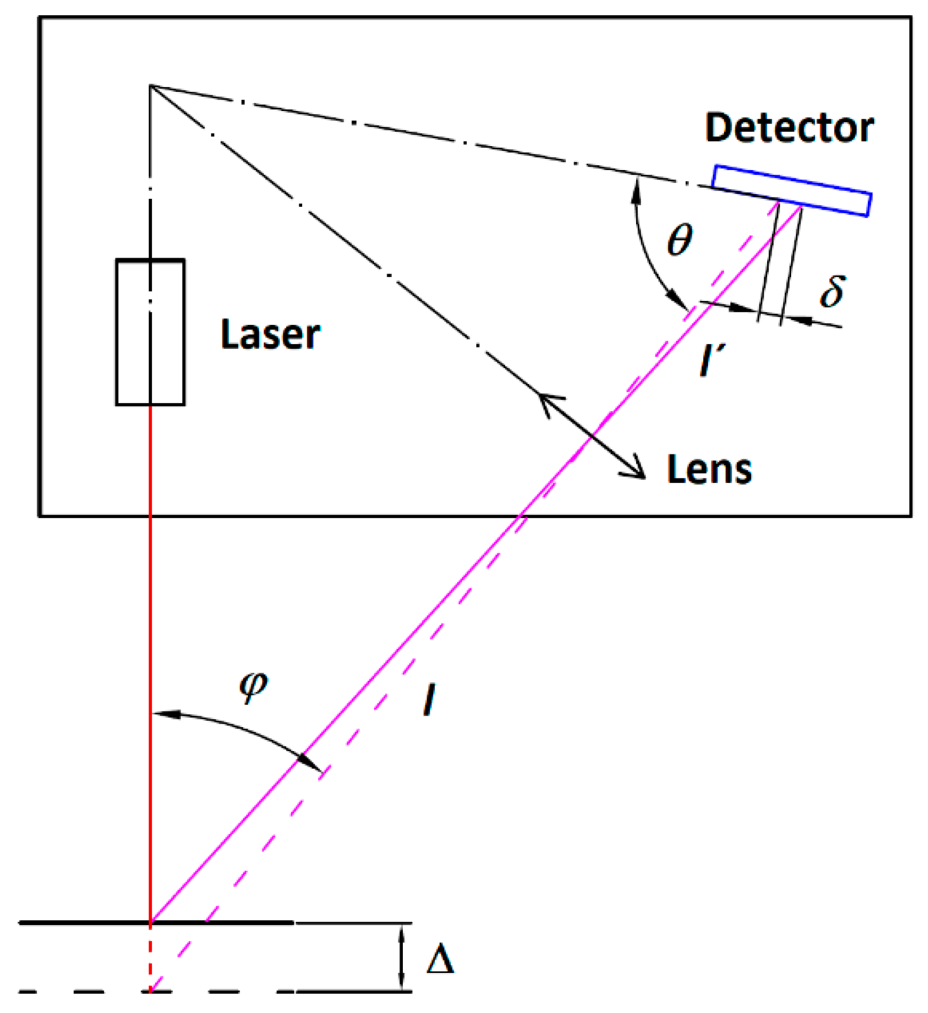
Figure 2.
Test scheme in clear weather conditions. (LiDAR rotation frequency: 2; 2.6; 3.5; 4.3; 5.5; 7 Hz; distances d: 1 to 6 m, every 1 m; target is a stationary placed sphere of 135 mm diameter).
Figure 2.
Test scheme in clear weather conditions. (LiDAR rotation frequency: 2; 2.6; 3.5; 4.3; 5.5; 7 Hz; distances d: 1 to 6 m, every 1 m; target is a stationary placed sphere of 135 mm diameter).
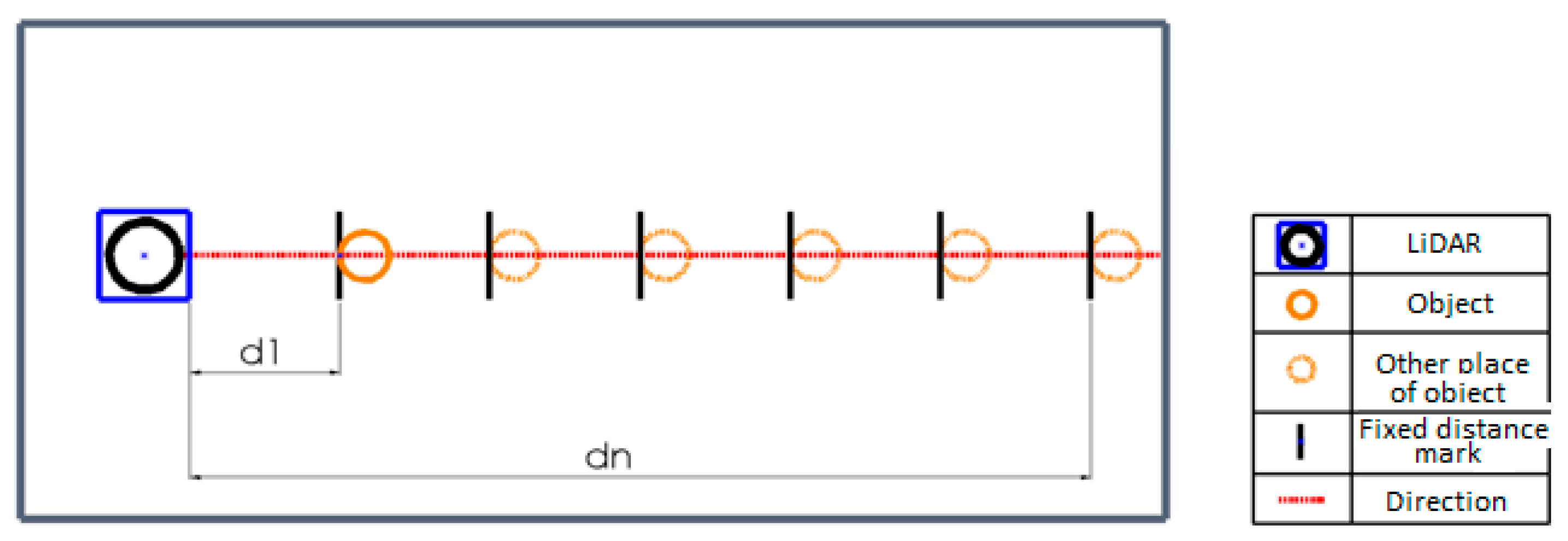
Figure 3.
Restored images of the object at a distance d = 1 m, at different scanning frequencies resulting in different amounts of image points (x-coordinate is the distance to left and right from central LiDAR fixed position).
Figure 3.
Restored images of the object at a distance d = 1 m, at different scanning frequencies resulting in different amounts of image points (x-coordinate is the distance to left and right from central LiDAR fixed position).
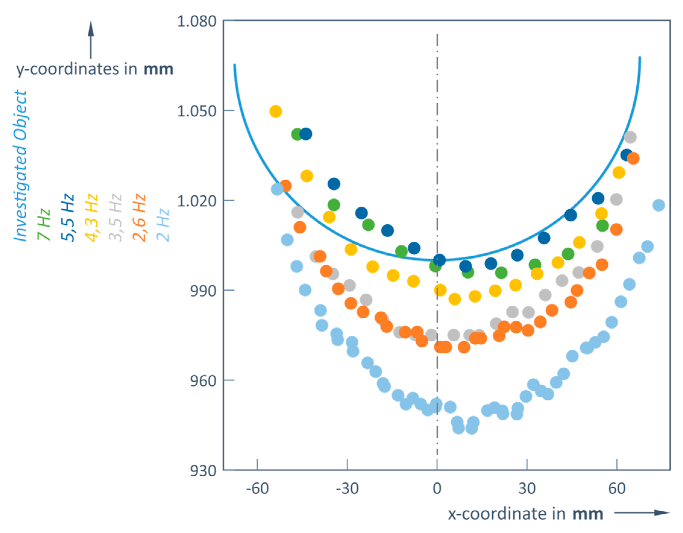
Figure 4.
Human silhouette (outlined in red) at 5 m distance from the LiDAR: recognized in the upper image (without rain) and not detected lower image with rain), while the tree is nearly imaged the same at both conditions (slightly different viewing angle at the two conditions).
Figure 4.
Human silhouette (outlined in red) at 5 m distance from the LiDAR: recognized in the upper image (without rain) and not detected lower image with rain), while the tree is nearly imaged the same at both conditions (slightly different viewing angle at the two conditions).
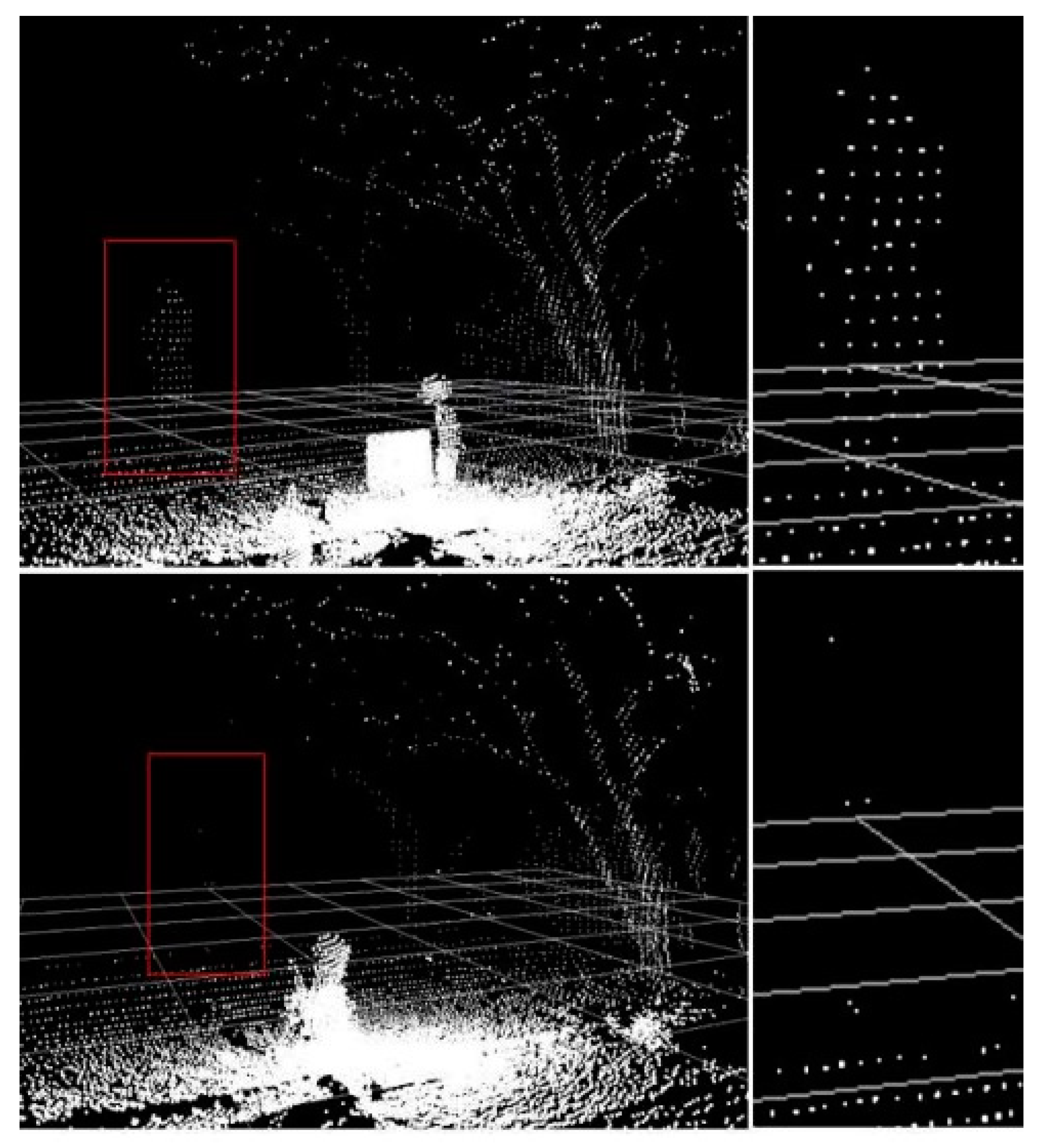
Figure 5.
Restored images of the object at a distance d = 6 m.
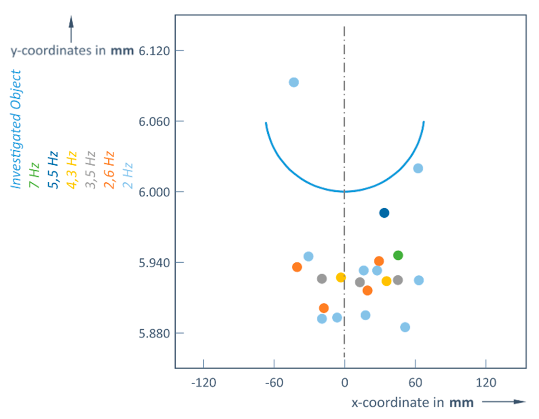
Figure 6.
Test scheme with artificial rain. LiDAR rotation frequency: 2; 2.6; 3.5; 4.3; 5.5; 7 Hz; Distances d: 1 ÷ 6 m, every 1 m; the measured object is a stationary ball of 135 mm diameter; measurement environment – rain intensity ~ 20 mm/h.
Figure 6.
Test scheme with artificial rain. LiDAR rotation frequency: 2; 2.6; 3.5; 4.3; 5.5; 7 Hz; Distances d: 1 ÷ 6 m, every 1 m; the measured object is a stationary ball of 135 mm diameter; measurement environment – rain intensity ~ 20 mm/h.

Figure 7.
Restored images of the object at a distance d = 1 m in rainy weather conditions.
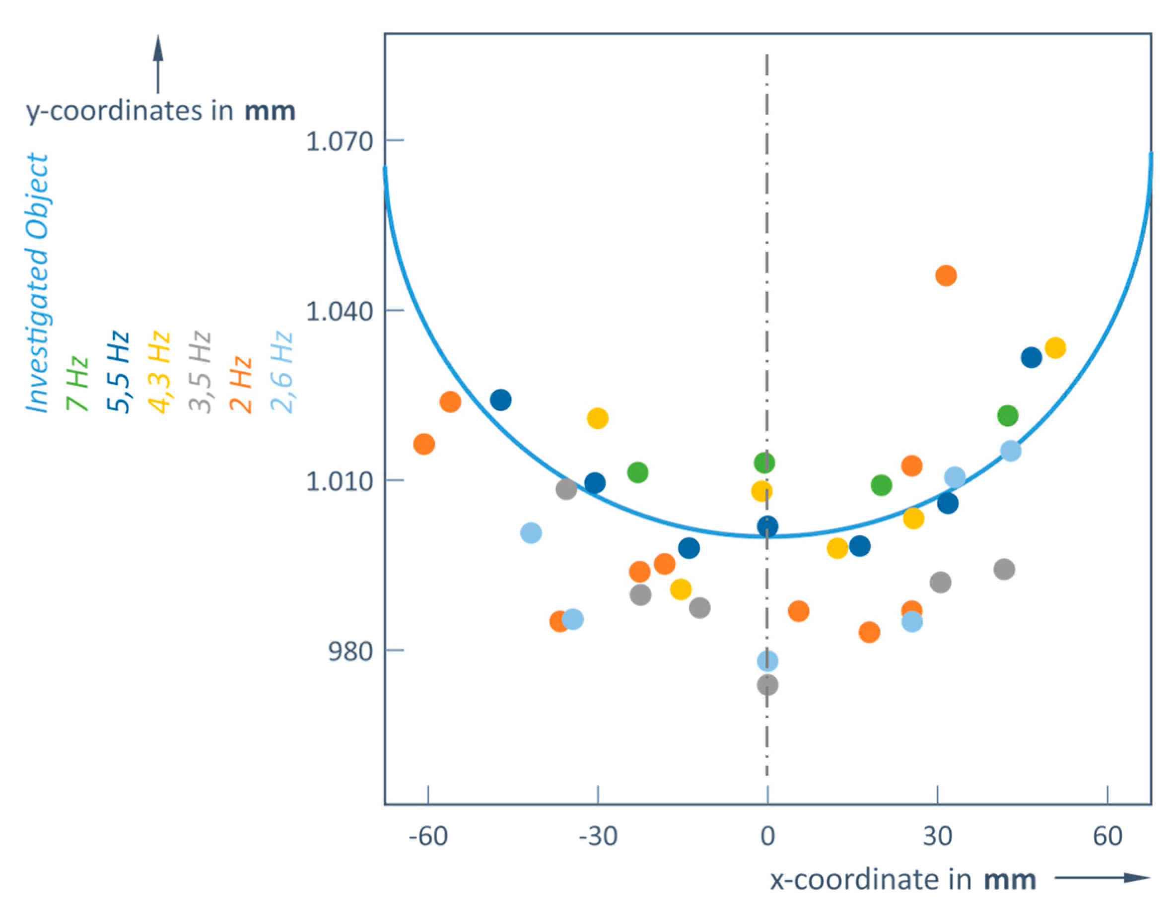
Figure 8.
Restored images of the object at a distance d = 6 m in rainy weather conditions.
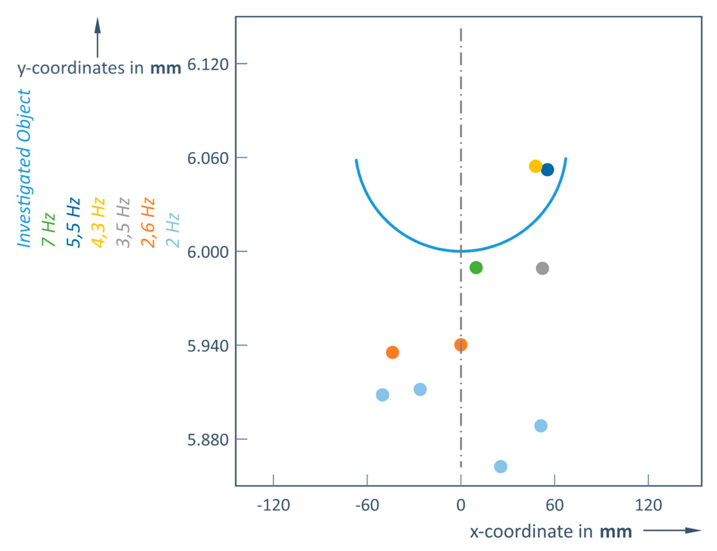
Figure 9.
Number of detected point’s vs scanning frequency f [Hz] and measurement distance d [m] without rain.
Figure 9.
Number of detected point’s vs scanning frequency f [Hz] and measurement distance d [m] without rain.
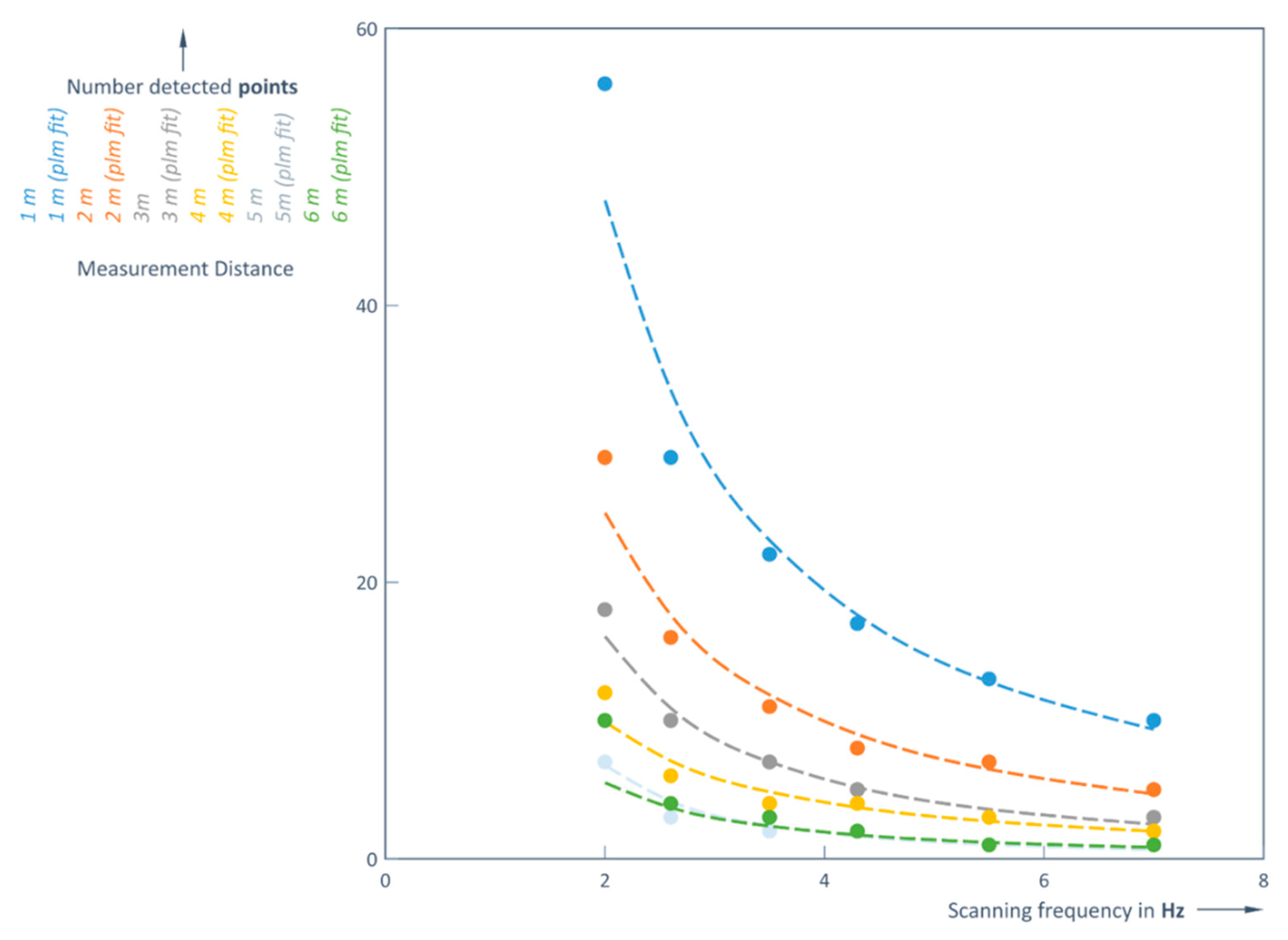
Figure 10.
Dependence on the number of detected points on scanning frequency f [Hz] and measurement distance d [m] in rainy weather conditions.
Figure 10.
Dependence on the number of detected points on scanning frequency f [Hz] and measurement distance d [m] in rainy weather conditions.
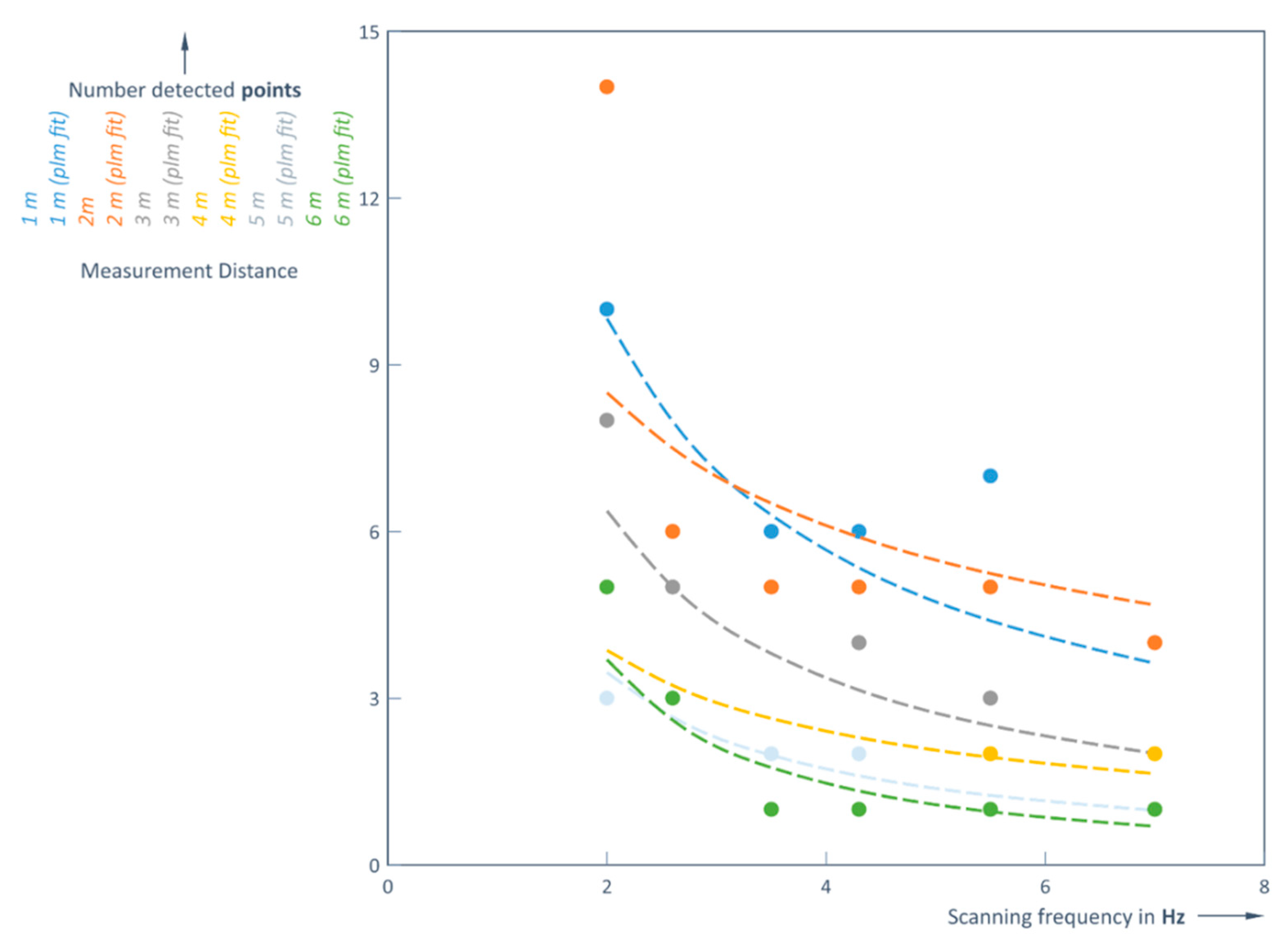
Figure 11.
Correlation between calculated and experimental number of detected points obtained from different scanning frequencies.
Figure 11.
Correlation between calculated and experimental number of detected points obtained from different scanning frequencies.
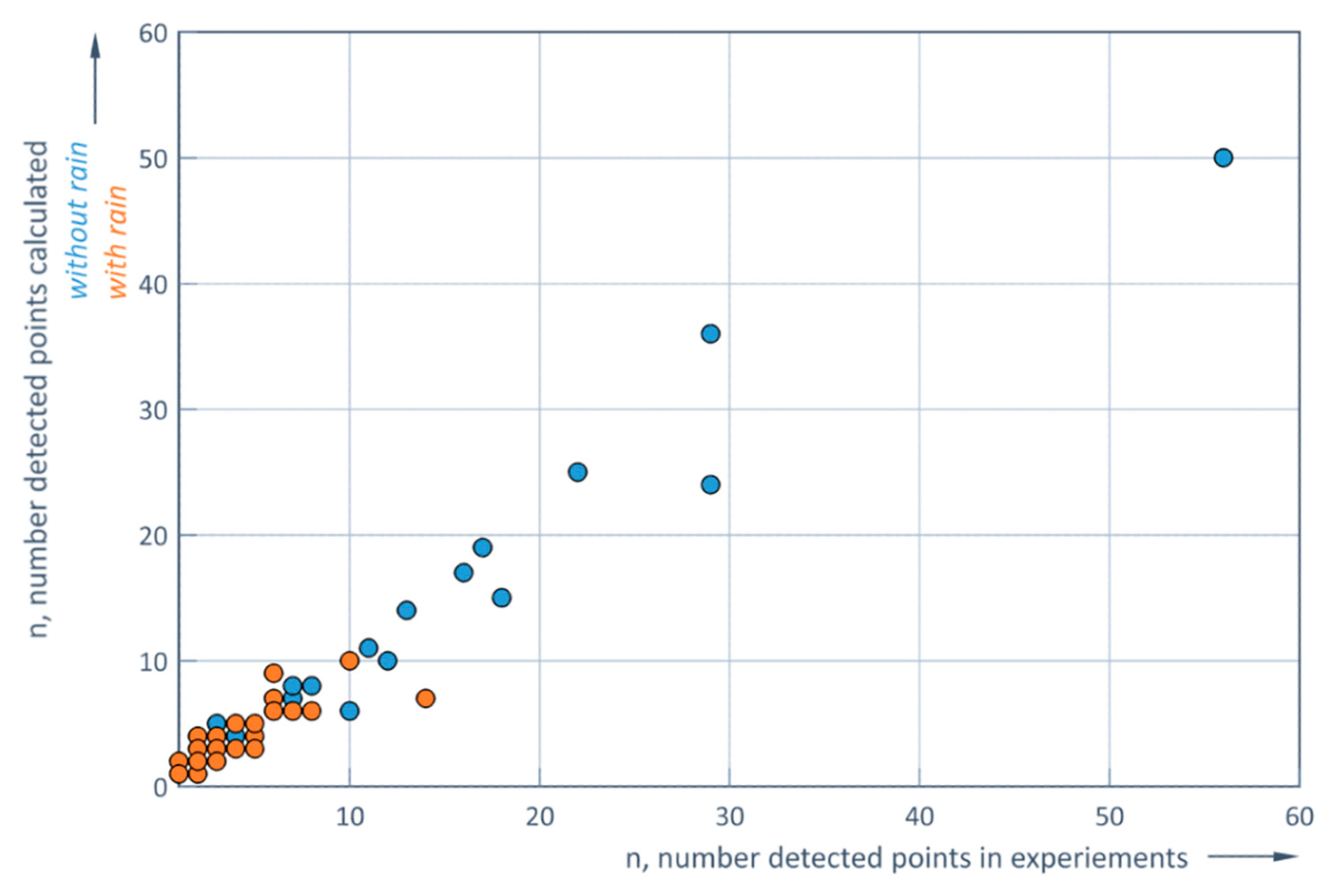
Figure 12.
Predicted and experimental number of recorded points depending on distance d [m] and LiDAR operating frequency f [Hz] in clear weather conditions.
Figure 12.
Predicted and experimental number of recorded points depending on distance d [m] and LiDAR operating frequency f [Hz] in clear weather conditions.
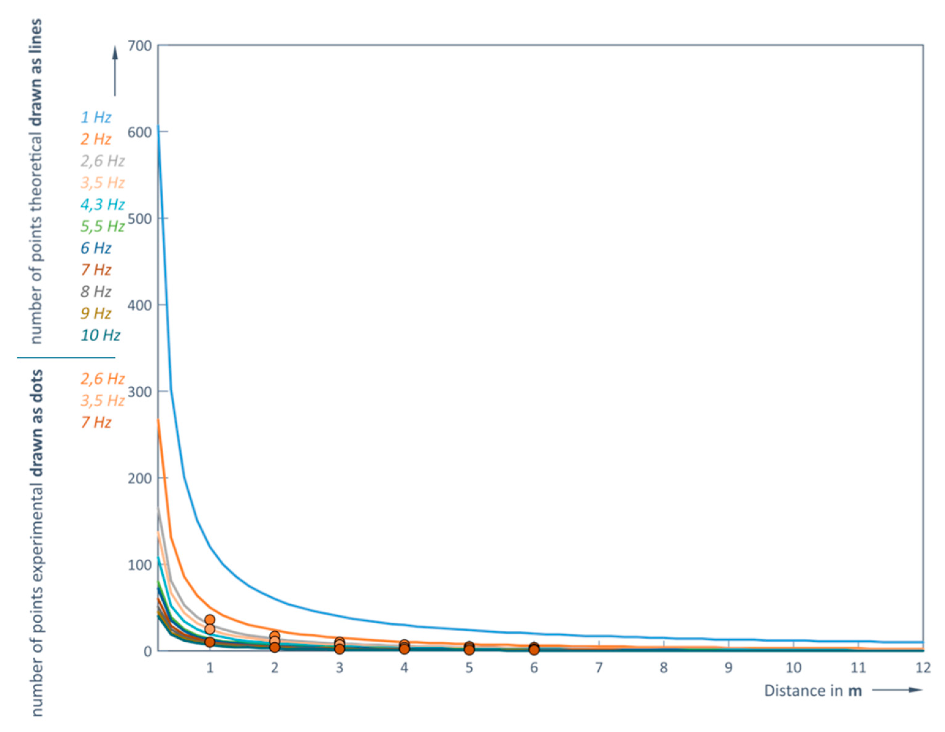
Figure 13.
Predicted and experimental number of recorded points depending on distance d [m] and LiDAR operating frequency f [Hz] in rainy weather conditions.
Figure 13.
Predicted and experimental number of recorded points depending on distance d [m] and LiDAR operating frequency f [Hz] in rainy weather conditions.

Figure 14.
RMS vs distance d [m] for different LiDAR operating frequencies f [Hz]: (a) clear weather; (b) rainy weather conditions.
Figure 14.
RMS vs distance d [m] for different LiDAR operating frequencies f [Hz]: (a) clear weather; (b) rainy weather conditions.
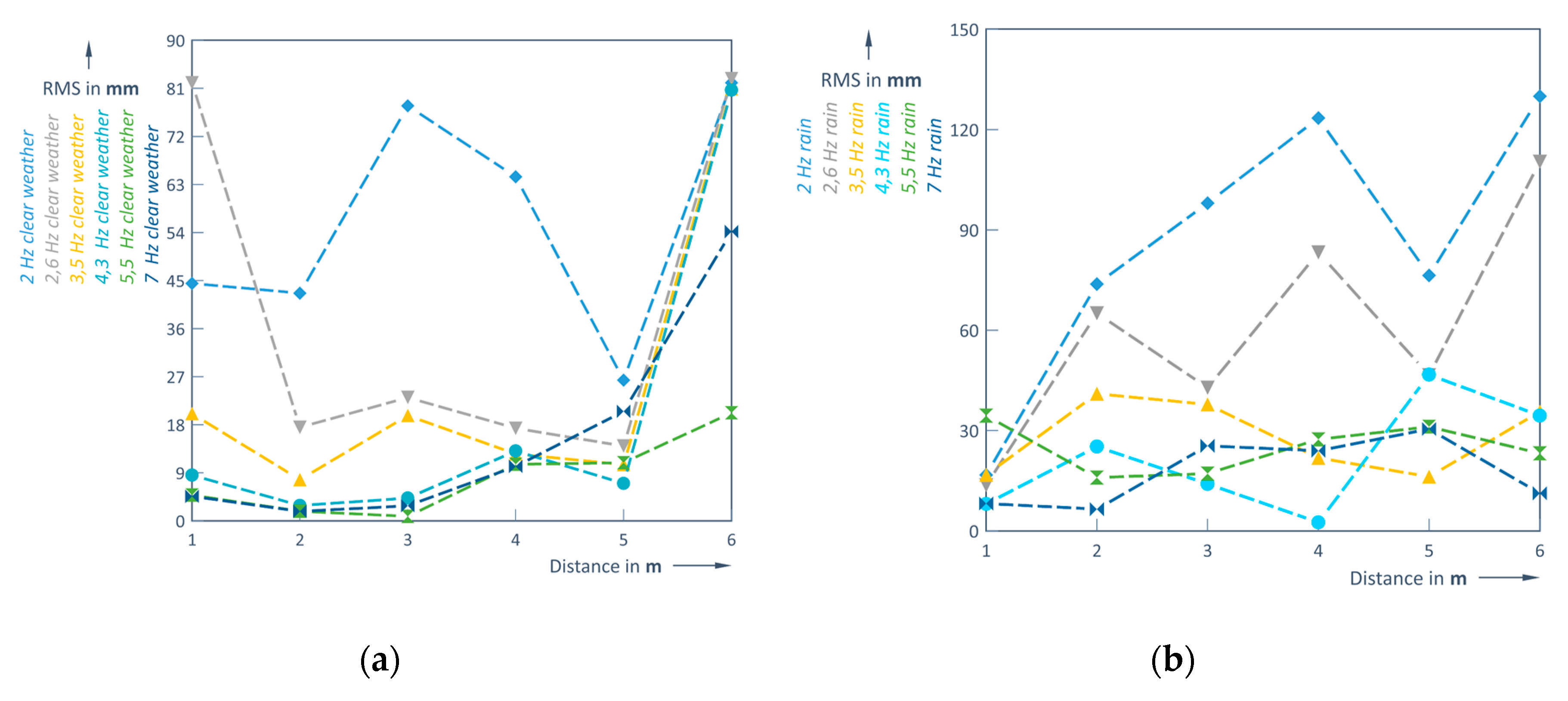
Figure 15.
RMS vs distance d [m]: (a) clear weather; (b) rainy weather conditions.

Figure 16.
Scatter diagram under clear weather conditions: (a) d = 1 m; (b) d = 6 m.
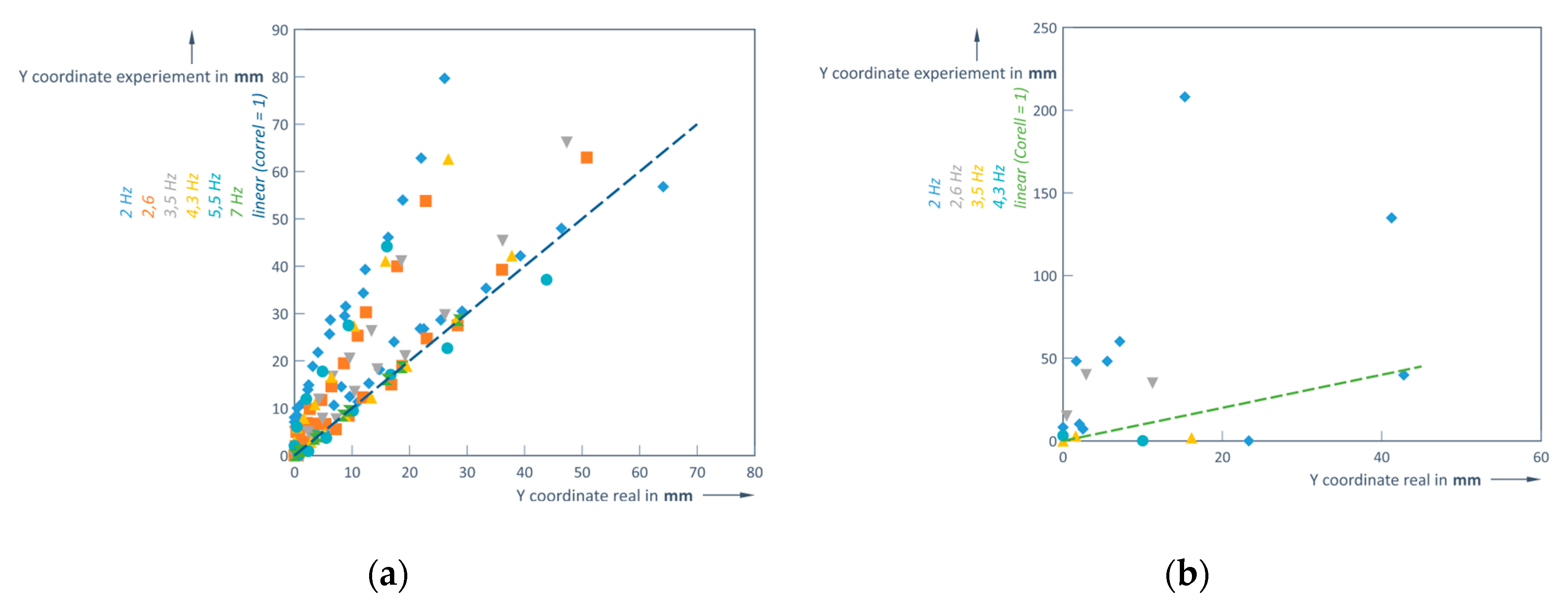
Figure 17.
Standard deviation without rain and with rain: at distances of 1 m; (b) d = 2 m, correspondingly.
Figure 17.
Standard deviation without rain and with rain: at distances of 1 m; (b) d = 2 m, correspondingly.
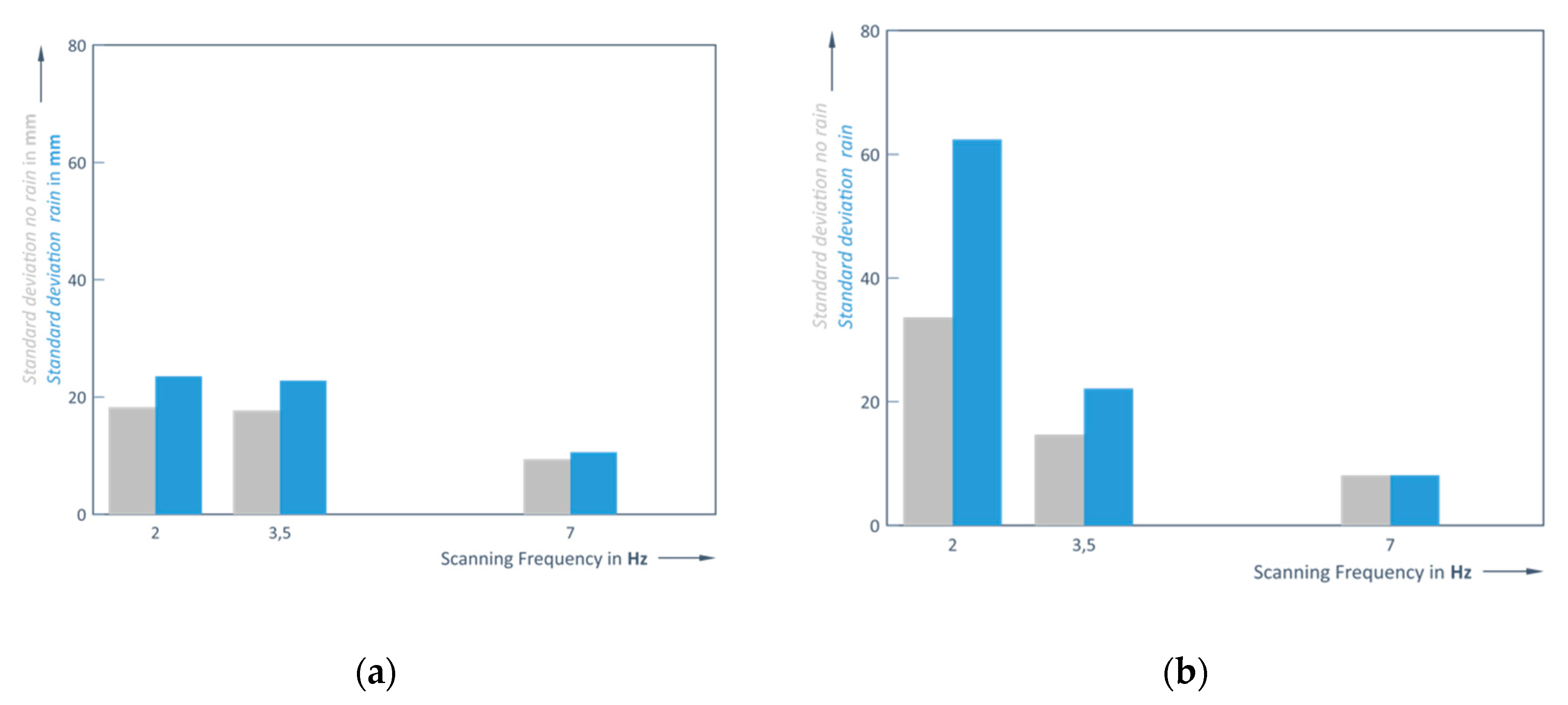
Figure 18.
Normal distribution CDF measured and theoretical values at a distance of 1 m for scanning frequency f of 2 Hz and 7 Hz.
Figure 18.
Normal distribution CDF measured and theoretical values at a distance of 1 m for scanning frequency f of 2 Hz and 7 Hz.
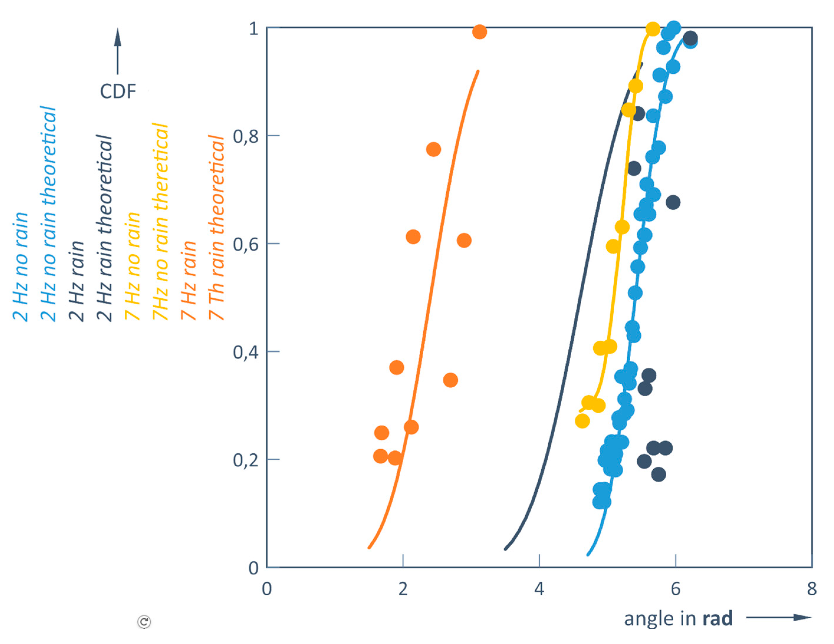

Table 1.
The results of the experiment at clear conditions and a distance d of 1 m.
| d, m | f, Hz | i, number of points | di = 1 mat, m | , mm | , mm |
|---|---|---|---|---|---|
| 1 | 2 | 49 | 0,944 | 44,467 | 7,837 |
| 2,6 | 29 | 0,971 | 23,097 | 5,946 | |
| 3,5 | 21 | 0,975 | 20,081 | 6,671 | |
| 4,3 | 17 | 0,987 | 8,564 | 3,796 | |
| 5,5 | 13 | 0,998 | 4,809 | 4,393 | |
| 7 | 10 | 0,996 | 4,589 | 2,886 |
Table 2.
The results of the experiment under clear conditions and a distance d of 6 m.
| d, m | f, Hz | I, number of points | di = 1 mat, m | , mm | , mm |
|---|---|---|---|---|---|
| 6 | 2 | 10 | 5,885 | 82,033 | 36,745 |
| 2,6 | 4 | 5,901 | 82,820 | 14,879 | |
| 3,5 | 3 | 5,923 | 80,886 | 3,402 | |
| 4,3 | 2 | 5,924 | 80,662 | 6,442 | |
| 5,5 | 1 | 5,982 | 20,227 | - | |
| 7 | 1 | 5,946 | 54,173 | - |
Table 3.
The results with rain at a distance of d = 1 m.
| d, m | f, Hz | I, number of points | di = 1 mat, m | , mm | , mm |
|---|---|---|---|---|---|
|
1 |
2 | 10 | 0,983 | 16,739 | 10,104 |
| 2,6 | 6 | 0,978 | 13,658 | 10,359 | |
| 3,5 | 6 | 0,974 | 16,735 | 8,589 | |
| 4,3 | 6 | 0,991 | 8,050 | 4,656 | |
| 5,5 | 7 | 0,998 | 4,418 | 3,925 | |
| 7 | 4 | 1,009 | 8,178 | 3,256 |
Table 4.
The results for rain at a distance of d = 6 m.
| d, m | f, Hz | I, number of points | di = 1 mat, m | , mm | , mm |
|---|---|---|---|---|---|
|
6 |
2 | 5 | 5,836 | 129,825 | 26,977 |
| 2,6 | 3 | 5,823 | 110,360 | 70,211 | |
| 3,5 | 1 | 5,989 | 35,633 | - | |
| 4,3 | 1 | 6,054 | 34,449 | - | |
| 5,5 | 1 | 6,052 | 23,182 | - | |
| 7 | 1 | 5,989 | 11,225 | - |
Table 5.
Predicted number of recorded points as a function of distance d [m] and scanning frequency f [Hz] in clear weather conditions (regarding Figure 12).
Table 5.
Predicted number of recorded points as a function of distance d [m] and scanning frequency f [Hz] in clear weather conditions (regarding Figure 12).
| D [m] | n @ 2 Hz | N @ 3.5 Hz | N @ 7 Hz |
|---|---|---|---|
| 1 | 56 | 22 | 10 |
| 2 | 29 | 11 | 5 |
| 3 | 18 | 7 | 3 |
| 4 | 12 | 4 | 2 |
| 5 | 7 | 2 | 1 |
| 6 | 10 | 3 | 1 |
Table 6.
Predictive number of recorded points depending on distance d [m] and scanning frequency f [Hz] in rainy weather conditions (regarding Figure 13).
Table 6.
Predictive number of recorded points depending on distance d [m] and scanning frequency f [Hz] in rainy weather conditions (regarding Figure 13).
| D [m] | n @ 2 Hz | N @ 3.5 Hz | N @ 7 Hz |
|---|---|---|---|
| 1 | 10 | 6 | 4 |
| 2 | 14 | 5 | 4 |
| 3 | 8 | 2 | 2 |
| 4 | 5 | 2 | 2 |
| 5 | 3 | 2 | 1 |
| 6 | 5 | 1 | 1 |
Disclaimer/Publisher’s Note: The statements, opinions and data contained in all publications are solely those of the individual author(s) and contributor(s) and not of MDPI and/or the editor(s). MDPI and/or the editor(s) disclaim responsibility for any injury to people or property resulting from any ideas, methods, instructions or products referred to in the content. |
© 2025 by the authors. Licensee MDPI, Basel, Switzerland. This article is an open access article distributed under the terms and conditions of the Creative Commons Attribution (CC BY) license (http://creativecommons.org/licenses/by/4.0/).
Copyright: This open access article is published under a Creative Commons CC BY 4.0 license, which permit the free download, distribution, and reuse, provided that the author and preprint are cited in any reuse.


