
Submitted:
11 April 2025
Posted:
11 April 2025
You are already at the latest version
Abstract
To investigate the fracture crack in the rear axle of a certain passenger car during accelerated life testing, a comparative testing analysis was conducted on this car after replacing its new rear axle and on a comparative car. Strain on the rear axle, vibration acceleration, and vehicle speed signal were measured for both cars. Using the cyclic stress-strain hysteresis loop equation and Neuber's Rule, the nominal strain histories obtained from tests were converted to local stress-strain responses at the fracture crack locations. Subsequently, the fatigue damage to the rear axles of both the target car and comparative car was calculated based on Morrow's mean stress correction model and Miner's linear cumulative damage rule. The frequency sweeping of vibration mode was performed on the car bodies and rear axles of both cars using electromagnetic exciters to establish the correlation between the vibration frequency of rear axle, the excitation frequency of PG durability road, and the body vibration frequency. The calculations of fatigue damage and the frequency sweep testing results indicated that the accumulated damage to the rear axle of the target car was primarily concentrated on the washboard road of the PG. On this road surface, the standard deviation of rear axle strain and the RMS value of acceleration were higher than those observed in the comparative car. At a test speed of 65 km/h, the excitation frequency of forced vibration caused by the washboard road was 24.1 Hz, which was close to the natural frequency of the vibration modes of target car's rear axle, leading to resonance. This resulted in the rear axle experiencing significant amplitude alternating stress, thereby causing the crack initiation of vibration fatigue.
Keywords:
crack initiation
; vibration fatigue
; rear axle
; accelerated life testing
; passenger car
; modal frequency sweeping
; resonance frequency
1. Introduction
The rear axle, as a critical load-bearing component of passenger cars, can precipitate severe traffic accidents if it fractures during vehicle operation [1]. The rear axle of a passenger car is subject to complex and variable loads over time due to road surface irregularities, vehicle acceleration and deceleration, steering, and braking [2]. These loads, which vary in magnitude and direction depending on driving conditions, subject the rear axle to alternating stresses, thereby inducing fatigue damage and creating conditions conducive to crack initiation [2,3]. The vehicle’s own weight, along with that of passengers and cargo, is transmitted through the suspension system to the rear axle, subjecting it to vertical pressure. Impacts caused by the road surface lead to dynamic changes in the vertical load [3]. The driving force output by the engine, transmitted through the drivetrain, generates torque in the rear axle, while braking forces acting in the opposite direction to travel induce shear and torsional stresses on the axle [4]. Lateral forces during vehicle cornering cause bending stresses in the rear axle, particularly during high-speed turns or abrupt braking, when lateral forces may significantly increase [1,2]. Under the influence of these alternating loads, the microstructure within the axle material undergoes cumulative damage [5]. In regions of stress concentration, such as at the axle shoulders, keyways, and surface defects, the movement of dislocations gradually forms microcracks, marking the initial stage of fatigue crack nucleation. As the number of load cycles increases, these microcracks gradually propagate under the influence of stress [6]. The direction of crack propagation is typically perpendicular to the direction of maximum principal stress, and the rate of propagation is influenced by factors such as stress amplitude, material characteristics, and environmental conditions [7]. When the crack extends to a certain extent, and the remaining load-bearing area of the rear axle is unable to sustain the applied load, a sudden fracture occurs [5,6,7]. Given that the reliability of the rear axle directly affects the overall performance and safety of the vehicle, the strength, stiffness, and fatigue life of the rear axle must meet design specifications.
Automobiles may be conceptualized as complex elastic systems. When time-varying operational loads are applied to these systems, multiple vibration modes are excited [8,9]. The dynamic response of the system at a point sufficiently distant from the loading point manifests as a stress-time history, which differs in amplitude, phase, and frequency when compared to the load-time history [10]. Such stress-time histories encapsulate two aspects: the effect of external loads and the dynamic response of the structure to these loads [11]. In practical measurements, external loads are often not directly observable; rather, their effects are measured at specific points on the structure [12,13]. The output response functions measured at these points are collectively referred to as stress-time histories, irrespective of whether they represent stress, strain, or other physical quantities indicative of structural stress, such as torque, force, or acceleration. The measurement of the natural frequencies of critical automotive components is employed to evaluate the dynamic characteristics of the vibration system [14]. The natural frequency refers to the first-order natural frequency, corresponding to the frequencies at which peaks occur in the frequency response curve, indicative of the natural frequencies of various modal orders. Resonance occurs when the system’s excitation frequency equals or approximates its natural frequency, leading to a maximal amplitude [15]. The frequency distribution of dynamic alternating loads coinciding closely with the frequency distribution of the structure’s natural frequencies can cause vibration fatigue damage due to resonance. Resonance fatigue is often related to component resonance or local resonance [16]. Dynamic load excitations frequently result in vibration coupling between localized modal responses and the loads, with damage typically occurring at regions of local resonance where strain is high and defects or stress concentrations exist, representing a combined effect of local resonance and stress concentration [12,14]. Therefore, when the system is subjected to external excitations, it is crucial to ascertain how close the excitation frequency is to the natural frequency of the structure to avoid resonance issues. In automotive design, it is typical to avoid resonance by ensuring a separation of 3-4Hz or 15%-20% of the natural frequency between the excitation and natural frequencies [14,15,16].
This study focuses on the occurrence of fracture cracks in the rear axle during accelerated life testing in a PG for a passenger car. Measurements were taken of the strain near the crack, axle end acceleration, and vehicle speed, among other test data. Furthermore, the rear axle was subjected to bench testing under longitudinal bending conditions to measure the maximum operational stress. The fatigue damage of the rear axle during the accelerated life test, the power spectral density (PSD), and the RMS value of the acceleration signal were calculated. Vibrational modal frequency sweeps were performed on the rear axle and the car body to identify the correlation between vibration frequencies and fatigue damage. Based on these findings, the crack initiation mechanisms of the rear axle were analyzed.
2. Fatigue Damage of Structures
The fatigue refers to the localized damage process in components caused by cyclic loading [17]. During the cycle of loading, localized plastic deformation occurs in areas of highest stress, leading to fatigue damage in components. Fatigue failure is one of the most common modes of failure, accounting for approximately 70-80% of total failure in various mechanical components [17,18]. Principally, fatigue fracture failure falls under the category of low-stress brittle fracture, and it is challenging to observe significant plastic deformation during fatigue since the deformation predominantly occurs at the inherent flaws of the structure [19]. The primary methods for predicting the formation of fatigue cracks include the nominal stress method and the local stress-strain method. A major limitation of the nominal stress method is its failure to account for the plasticity at the notches, whereas the local stress-strain method reasonably considers the effects of localized plasticity and local mean stress at the notch roots [18,19,20]. Although most components nominally experience cyclic elastic stress, components with notches, welds, or other stress concentrators undergo localized cyclic plastic deformation, thereby making the local stress-strain method more effective for predicting the fatigue life of components. Under random loading, each hysteresis loop formed in the material constitutes a fatigue damage unit [21]. The rainflow counting method can process the load time history into a rainflow cycle counting matrix of amplitude-mean-cycles [22]. With known material strain histories, using the material cyclic stress-strain curve and the rainflow counting method for local stress-strain analysis enables the determination of the number of each hysteresis loop, which lays the foundation for calculating fatigue life [23]. The local stress-strain analysis is based on the cyclic stress-strain curve of the material, its memory characteristics, and the rainflow cycle counting method. Its purpose is to determine the number of hysteresis loops formed in the material under known load or strain histories [22,23]. The rainflow counting method is a statistical approach for fatigue analysis based on the characteristics of the material stress-strain hysteresis loops. It effectively converts complex load time histories into a series of stress amplitude-mean-cycles matrices through the rainflow cycle counting process, as illustrated in Figure 1 [21,22,23,24]. During the cyclic loading process, the relationship between local stress and strain variations and the measured nominal stress and strain variations is depicted in Figure 2.
Due to the difficulty of affixing strain gauges directly over the crack on the rear axle, it is only feasible to place them in proximity to the crack. In such circumstances, it becomes necessary to estimate the local stress-strain response at the crack based on the actual signals measured by the strain gauges [25]. The Neuber’s Rule can be applied to convert the experimentally measured nominal strain spectrum into a local stress-strain response at the location of the crack, as follows:
Where and represent the local stress and strain amplitudes at the crack, respectively, while and are the nominal stress and strain amplitudes measured by the strain gauge. denotes the fatigue notch factor, which is the ratio of the fatigue strength of a smooth specimen to that of a notched specimen.
The fatigue notch factor can be calculated using the Neuber-Kuhn formula:
Where is the theoretical stress concentration factor (the ratio of the maximum local elastic stress to the nominal stress), is the radius of the fillet at the notch root, and is a material constant related to the material’s ultimate strength and heat treatment condition.
Based on the hysteresis loop curve equation, the relationship between local stress and strain amplitudes at the position of the crack on the rear axle is given by:
Where E is the modulus of elasticity, is the cyclic strength coefficient, and is the cyclic hardening exponent.
Transforming Equation (3) results in:
Introducing Equation (1) into Equation (4) yields:
By analyzing the strain time history measured by the strain gauges on the rear axle, the individual hysteresis loops and the corresponding stress and strain amplitudes at the location of the strain gauge can be determined [26,27]. Substituting and into Equation (5) to obtain , and then substituting into Equation (3) to obtain , allows for calculating the local stress-strain response at the crack location of the rear axle in terms of the coordinates of the hysteresis loop vertices ().
In the local stress-strain method, the material’s fatigue strength is represented by the strain-life curve [6]. In a double logarithmic coordinate system, the components of the elastic strain amplitude and plastic strain amplitude within each hysteresis loop correlate linearly with the corresponding fatigue life, and their power law expressions can be represented as:
Where is the fatigue strength coefficient, is the fatigue plasticity coefficient, is the fatigue strength exponent, is the fatigue plasticity exponent, and is the fatigue life for crack initiation.
The total strain amplitude is the sum of the elastic and plastic strain amplitudes, as:
The strain-life curve is typically derived from material tests conducted under symmetric cyclic strain control, where both the mean stress and mean strain are zero. However, in practical load signal processing, scenarios often arise where the mean stress and strain are not zero [5,6,7]. While the effects of mean strain can generally be disregarded, it is necessary to correct for the impact of mean stress. Mean stress significantly influences fatigue life by altering the effective stress level within the material and the rate of crack propagation. The degree to which mean stress affects fatigue life is determined by a combination of factors including material properties, type of load, and environmental conditions. In engineering practice, it is essential to integrate correction models with experimental data to optimize design under specific operational conditions, thus ensuring the safety and reliability of engineering structures. When cyclic loading includes a mean tensile stress, the effective stress level inside the material significantly increases. This elevated stress level accelerates crack propagation, thereby substantially reducing the material’s fatigue life. As the magnitude of the mean tensile stress increases, the fatigue life of the material exhibits a marked nonlinear decline. Conversely, mean compressive stress inhibits crack propagation and effectively extends the fatigue life of the material. This is because compressive stress causes crack tips to close, significantly reducing stress concentration and delaying further crack propagation. In predicting fatigue life, accurate assessment of material performance under non-zero mean stress requires the use of correction models to equate non-zero mean stress to symmetric cyclic stress. The Morrow’s mean stress correction model is a pivotal method in addressing the effects of mean stress under asymmetric cyclic loading in fatigue life prediction. This model is widely used in engineering and focuses on modifying the strain-life relationship to reflect the cumulative effect of mean stress on material fatigue damage. The Morrow’s mean stress correction model is illustrated in Figure 3. The Morrow’s mean stress correction equation is expressed as follows:
Where represents the mean stress in the presence of a hysteresis loop.
The Morrow’s equation accounts for the influence of mean stress on fatigue life and modifies the elastic component of the strain-life curve. This equation is extensively applied to steel materials. Under dynamic loading, the rear axle of a car experiences fatigue damage in each rainflow cycle [6]. Using known strain-life curves and the number of rainflow cycles, it is possible to calculate the fatigue damage induced by each rainflow cycle. Assume that a load history generates k rainflow cycles in the material, with the coordinates of each cycle’s two vertices represented as and , where i = 1, 2, ..., k, as shown in Figure 4.
The mean stress and strain range for each rainflow cycle are given by:
By substituting Equations (10) and (11) into the Morrow’s mean stress correction Equation (9), we obtain:
From Equation (12), the crack initiation life for each rainflow cycle i = 1, 2, ..., k can be calculated. Assuming that the fatigue damage caused by the -th stress amplitude level is denoted as , we have
Where k is the stress amplitude level, and is the number of rainflow cycles at the -th amplitude level.
Using Miner’s linear cumulative damage rule, the total fatigue damage D is accumulated from all amplitude levels:
Theoretically, when the total cumulative damage D equals 1, fatigue failure occurs in the rear axle, marked by the appearance of engineering cracks. Currently, there is no uniform standard for the length of engineering cracks, which typically range from 0.1 to 2 mm.
The suspension system of the test car features a MacPherson strut-type independent front suspension. The rear suspension is a longitudinal trailing arm-type semi-independent suspension, consisting of a torsion bar and a U-shaped shell surrounding the torsion bar, connected to the lateral bent arms. Each bent arm attaches to the car frame at one end and to the wheel at the other, with the U-shaped shell and torsion bar situated in the middle of the bent arm. As the left and right wheels move vertically, the rear axle absorbs some of the vibrations, maintaining a degree of body balance and achieving vehicle stability. The material used for the rear axle is 45 steel plate, with a fabricated structure, a yield strength of 355 MPa, and a tensile strength of 600 MPa. Material-related parameters used in the damage calculations are provided in Table 1.
2. Load Testing and Damage Calculation
2.1. Load Measurement of PG Durability Roads
Accelerated life testing in PG serves as a crucial method for assessing and evaluating the durability and reliability of automotive components. This testing approach can simulate a variety of complex operating conditions that a vehicle may encounter during actual use in a relatively short period, thereby accelerating the aging and fatigue damage of the components. In these PG accelerated life tests, the rear axle frequently incurred damage to rubber casings and developed cracks. The majority of these tests were conducted over distances ranging from 8,000 to 13,000 km, with high repeatability. The comparative car equipped with the same model of rear axle were also tested under similar conditions for comparative validation. The findings indicated that cracks in the rear axle of the target car appeared after approximately 9,600km of durability bad road driving in the PG; whereas, the comparative car continued up to 30,000 km without any axle failures, successfully passing the validation test. To analyze the initiation of crack formation in the target car’s rear axle, load measurements were carried out concurrently with the comparative car. Strain gauges were affixed at three different points near the crack, site of stress concentration, and significant deformation to measure local strain in the rear axle. These specific measurement points are shown in Figure 5. Additionally, accelerometers were installed at the ends of the rear axle to record the vibration acceleration signals. Figure 6 and Figure 7 illustrate the data acquisition system and the actual car test on the washboard road surface in the PG, respectively. Time-domain data collected from the PG durability road tests are presented in Figure 8, Figure 9 and Figure 10.
2.2. Stress Measuring for Rig Test
The maximum operational stress under longitudinal bending conditions for the rear axles of both the target and comparative cars was measured. The experiment was conducted on a test rig at Tao Company, following the rear axle test operation protocol. The rear axle was mounted on the test rig, with the lever arm fixed at the hub axle base as shown in Figure 11. The testing condition was a longitudinal force bending test, with a loading torque of 800Nm and a frequency of 35Hz. Loading was applied to the axle body using an electromagnetic vibrator via the lever arm. Stress testing on the rear axles was conducted using the electrical resistance strain gauge method, with real-time recording of strain signals at various test points via a data acquisition system. The stress at each measurement point was calculated using Hooke’s Law from the strain and the material’s modulus of elasticity, with the maximum stress values at each point presented in Table 2.
The stress values at three measurement points on the target car’s rear axle were found to be consistently higher than those on the comparative car. At measurement point 2, the maximum principal stress for the target car was 160MPa, compared to 135MPa for the comparative car, representing increases of 30.4% and 15.2% in maximum principal stress and Von Mises stress, respectively, relative to the comparative car. The results of the longitudinal bending tests on the rear axles of both cars were consistent with those obtained from the PG durability road tests.
2.3. Calculation of Fatigue Damage
In order to estimate the service life of structures, conduct fatigue reliability analyses, and perform fatigue testing of components, it is essential to have a fatigue load spectrum that reflects the actual operating conditions. Due to the randomness of the measured stress-time history and the complexity of real-world operating conditions, it is necessary to simplify the stress-time history for convenience in experimentation and to reduce the duration of tests, thus obtaining a “typical load spectrum” that accurately represents true conditions. Given the vast amount of data that can be collected in just a few minutes, often comprising thousands of data points, the identification and counting procedures should employ automated methods, utilizing computer processing. nCode Glyph Works is a powerful data processing system primarily used for durability analysis and digital signal processing, capable of handling data from multiple sensors and supporting the analysis of time series and PSD data. Glyph Works facilitates the prediction of fatigue life, particularly through strain life analysis, aiding engineers in better understanding and predicting the reliability of components, optimizing designs, and reducing both development costs and time. Data collected during tests may be affected by environmental factors such as temperature, humidity, and magnetic fields, leading to issues with zero drift, spikes, and trends in the data, necessitating the preprocessing of raw measurement data to ensure the accuracy of test results. Glyph Works is used to establish a data preprocessing model as shown in Figure 12. During the data preprocessing process, correct test data are obtained by correcting for various data biases through methods such as changing means, filtering, and removal, subsequently allowing for the calculation of fatigue damage using Glyph Works, with the established calculation model shown in Figure 13. Figure 14 displays a comparison of the total cumulative damage between the comparative car and the target car over one test cycle in the PG, with the distribution of damage across various road surfaces in the PG presented in Table 3.
As evidenced by Table 3, the damage on the PG durability road is predominantly concentrated on the washboard, stone block, and twisted road. Among the three measurement points, the damage on the washboard road for the target car consistently exceeds that of the comparative car. Conversely, on the stone block and twisted road, the target car exhibits less damage than the comparative car. Notably, the washboard road contributes the most to the damage of the rear axles of both cars. On the washboard road, the damage ratio at measurement point 1 for the target car exceeds 80%, while for the comparative car, it surpasses 50%. Furthermore, at measurement points 2 and 3 for the target car, the damage ratios exceed 90%. For the comparative car, the damage ratio at measurement point 2 is over 80% and at measurement point 3, it is more than 60%, as depicted in Figure 15, Figure 16 and Figure 17.
Due to the significant levels of damage sustained by the rear axle on washboard road, this type of road surface has been prioritized for assessment in the current test study. A washboard road consists of a series of raised sections, each resembling a sine wave, with a height of 25mm, a length of 360mm, and a spacing of 750mm between peaks. This road surface is employed for automotive vibration and reliability testing. The cross-sectional profile of a washboard road is illustrated in Figure 18.
As the spacing between the protrusions on a washboard road is fixed, a car traveling over this surface at a constant speed will experience forced vibrations triggered by these protrusions. The fundamental frequency f of vibration, induced by the washboard road, can be calculated as follows:
Where f is the excitation frequency in Hz and v is the vehicle speed in km/h over the washboard road.
The standard deviation of strain measures the variability in local deformation of the rear axle, which is directly associated with fatigue damage under dynamic loading conditions. A higher standard deviation of strain indicates greater dispersion in the amplitude of plastic strain, leading to a more rapid increase in damage variables, thereby exacerbating fatigue damage and typically reducing the fatigue life. Statistical data from the PG featuring a washboard road show that the target car exhibits the highest standard deviation of strain at a speed of 65km/h, while the comparative car reaches its maximum at 60 km/h, as shown in Table 4.
The RMS value of vibration acceleration is a critical parameter representing the energy intensity of random vibrations and is commonly used to assess the fatigue life of structures under vibration environments. Higher RMS values indicate greater vibration loads on a structure or component, resulting in larger stress amplitudes. The stress amplitude is a principal factor in the onset of fatigue damage, leading to more rapid accumulation of fatigue damage. The statistical results of RMS values of vibration acceleration on a washboard road are documented in Table 5.
In the context of accelerated vibration fatigue testing, Glyph Works is adept at generating test specifications based on time series and PSD data. It computes the shock response spectra and the spectra of fatigue damage, thereby assessing the durability of components. The PSD model of the acceleration response established using Glyph Works is illustrated in Figure 19. The PSD represents the average power distribution within a unit frequency bandwidth. The peaks in the PSD are local maxima in the power distribution across the frequency domain, signifying the most concentrated energy frequency points. These peaks reflect the characteristic concentration of energy at specific frequencies, where the peak frequencies are typically the fundamental or harmonic frequencies of the signal. Due to the interaction between the input signal and the system, the output signal includes components that are integer multiples of the input signal’s frequencies, resulting in a multiplication relationship of peak frequencies in the PSD graph. Figure 20 and Figure 21 depict the longitudinal and vertical acceleration PSD of the PG durability road, respectively.
On the washboard road, the damage distribution at three measurement points on the rear axle of the cars varies with speed, as shown in Figure 22, Figure 23 and Figure 24. At the target car’s three measurement points, the maximum damage occurs at 65km/h, with values of 7.553×10⁻⁷, 3.177×10⁻⁶, and 1.386×10⁻⁶, respectively. For the comparative car, the greatest damage at its three measurement points occurs at 60km/h, with damages of 1.660×10⁻⁷, 1.081×10⁻⁶, and 0.365×10⁻⁶, respectively. The interaction between the system’s natural frequencies and the excitation frequencies may induce multi-order resonance frequencies. Since systems often possess multiple natural frequencies, which may relate to each other as integer multiples, this relationship is reflected in the PSD as multiple peak frequencies. The PSD curves from Figure 20 and Figure 21 indicate that the working amplitude frequency of the rear axle’s acceleration response is around 24Hz. When the test car travels over a washboard road at speeds of 60km/h and 65km/h, the forced vibration excitation frequencies for the washboard road, calculated using Equation (15), are approximately 22.2Hz and 24.1Hz, respectively. The closeness of the road excitation frequency to the rear axle’s working amplitude frequency induces resonance in the rear axle, resulting in significant strain amplitude and fatigue damage at these speeds.
3. Analysis of Vibration Modes
3.1. Determination of Modal Parameters
The modal characteristics are inherent vibratory properties of a structural system [8,9]. In the case of linear vibrational systems, there exist characteristic inherent vibrational modes, and the response of the system is a linear combination of these modes. The free vibration of a linear system can be decomposed into several orthogonal single-degree-of-freedom vibrational systems, which manifest as vibrational patterns at different frequencies [10]. Each mode corresponds to a specific set of natural frequencies, damping ratios, and mode shapes. The natural frequency is the frequency of vibration in that mode, the damping ratio describes the characteristics of vibrational energy dissipation, and the mode shape represents the spatial distribution of vibrational displacement. These modal parameters can be obtained through computational or experimental analysis [11,12,13]. The objective of modal analysis is to identify the modal parameters of the system, providing a basis for the analysis of structural system vibrational characteristics, and for the prediction and diagnosis of vibrational faults. Modal analysis is based on the theory of vibration. Initially, a physical parameter model of the structure is established, which is a vibrational differential equation concerning displacement, characterized by mass, damping, and stiffness parameters. Subsequently, the characteristic value problem is studied to obtain eigenvalues and eigenvectors, leading to the determination of modal model parameters, such as modal frequencies, modal vectors, modal damping ratios, modal mass, and modal stiffness [14,15]. By measuring the system’s transfer function, information such as the system’s frequency response and damping ratio can be obtained, thereby facilitating an understanding of the system’s vibrational characteristics and stability [15,16,17]. This knowledge is crucial for the design and optimization of various dynamic systems. The transfer function is used to describe the system’s response to input signals or the system’s frequency response [13,14]. It is derived using the Laplace transform, which is suitable for describing the dynamic characteristics of a system–specifically, how the system responds to time-varying inputs. For linear time-invariant systems, the relationship between input x(t) and output y(t) can be described by a constant-coefficient linear differential equation:
Where an, an-1, …, a0 and bm, bm-1, …, b0 are the physical parameters of the system.
For linear time-invariant systems, assuming initial conditions are zero, applying the Laplace transform to both sides of the differential equation yields:
Consequently, the transfer function H(s) of the system is
Where s is the complex frequency variable, and the power n of the denominator s indicates the order of the transfer function.
By conducting a frequency domain analysis of the transfer function, the system’s response to specific frequency input signals can be determined.
Substituting into Equation (18) results in the frequency response function (FRF):
Where is the imaginary unit, with , represents the angular frequency, is the system’s FRF,, .
Therefore, the FRF is a representation of the transfer function in the frequency domain, quantifying the system’s output Fourier transform relative to its input Fourier transform. The Fourier transform facilitates the conversion of time-domain signals into frequency-domain signals, which is utilized to analyze the system’s frequency domain characteristics. The FRF is an inherent property of the system, related to the system’s own characteristics and independent of external factors such as excitation and response. Any complex high-order vibrational system consists of a combination of first-order and second-order systems connected in series, parallel, or through feedback. A typical second-order system transfer function is:
In this equation, m denotes the system’s mass, c the viscous damping, and k the system stiffness. Define , where is the natural frequency of the undamped system, and is the critical damping value; is the damping ratio, calculated as .
The relationship between amplitude and frequency for a second-order vibrational system is described by:
At , the system experiences resonance, where the amplitude-frequency characteristic peaks, and the amplitude reaches its maximum. The characteristics of the resonance amplitude not only form the basis for efficient energy transfer but also represent a potential risk source.
The dynamic response y(t) of a multi-degree-of-freedom vibrational system can be decomposed into a linear combination of various order vibrational modes, indicating that the system’s vibration comprises a superposition of multiple order natural frequencies and mode shapes.
Where represents the mode shape of the ith order; and are the amplitude and phase angle of the corresponding mode; is the frequency of the ith order mode.
During modal analysis of a multi-degree-of-freedom vibrational system, by solving the characteristic value equation, one can precisely determine the system’s natural frequencies and mode shapes. The relationship among the modal parameters is described by
Where K is the system’s stiffness matrix, and M is the mass matrix.
Increasing stiffness leads to a higher resonance frequency and reduces the amplitude of the FRF at lower frequencies. Adding damping slightly decreases the resonance frequency, but its primary effect is to reduce the amplitude at the resonance point and smooth the phase change. Increasing mass decreases the resonance frequency and also lowers the amplitude of the FRF at higher frequencies.
3.2. Estimation of Modal Parameters
The central aspect of frequency-domain modal testing involves the measurement of the FRF and curve fitting of the measured data. To measure a system’s FRF, it is essential to record both the input (excitation signal) and output (response signal) of the system. By fitting experimental data to the response function, a series of modal parameters can be extracted, including natural frequencies, damping ratios, and mode shapes. This method of extracting parameters through experimental modal analysis is highly accurate in practical engineering applications. The most common form of experimental modal analysis is the rational fraction polynomial form, which clearly depicts the poles and their conjugates. The estimation of point-to-point FRF involves applying an excitation at point j in the system and measuring the response at point i. For a specific i-j (input-output) configuration, the FRF is an estimation of the transfer function along the axis, defined as follows
In this equation, Hij(jω) is the FRF between response degree of freedom i and reference degree of freedom j; N is the number of vibrational modes contributing to the dynamic response of the structure within the considered frequency range; rijk is the residue of mode k; λk is the pole of mode k; and * denotes complex conjugate.
The poles λk in Equation (24) can be expressed as
Or
Where is the damped natural frequency of mode k, is the undamped natural frequency of mode k, is the damping factor for mode k, and ζk is the damping ratio for mode k.
Parameter estimation involves adjusting the parameters in the model so that the model’s predicted data matches the measured data, thereby accomplishing the identification of modal parameters. The measurement of the test signal’s FRF is carried out using a spectrum analyzer, and the estimated modal parameters are determined through curve fitting using modal analysis software. Once the modal parameters are estimated, the vibration characteristics of the structure can be described through the mode shapes.
3.2. Frequency Sweeping of Vibrational Mode
The modal frequency sweeping was conducted on both the target car and the comparative car to identify the modal parameters of their bodies and rear axles. This analysis aimed to discern the differences in the vibrational frequencies of the rear axles between the two cars, as well as their relationship to the body vibration frequencies. During the frequency sweeping of vibrational mode tests, all four wheels of each test car were elevated to a specified height and placed upon steel boxes. Electromagnetic exciters were initially positioned on either side of the rear axle to stimulate vibrations, followed by their placement at the rear-left and front-right positions of the car body to induce vertical vibrations. Acceleration sensors recorded the vertical vibrational accelerations. At the time of testing, both cars were unladen, and tire pressures were adjusted to the values specified by technical requirements. Modal transfer functions and mode shapes for the target car’s body and rear axle are presented in Figure 25, Figure 26, Figure 27, Figure 28 and Figure 29, while those for the comparative car are shown in Figure 30, Figure 31, Figure 32 and Figure 33. The modal parameters and mode shapes were identified through fitting the modal transfer functions, establishing the system’s natural frequencies or damping characteristics. Results of the modal parameter frequency sweeping are detailed in Table 6.
From the results of the modal frequency sweeping tests, it is evident that the first-order torsional modal frequency of the target car’s body is 3.91Hz higher than that of the comparative car, and the vertical vibrational modal frequency of the rear axle is 3.37Hz higher. Structurally, this suggests that the stiffness of the target car’s body and the rigidity of its rear axle suspension are greater than those of the comparative car. Given that the cars were unladen during these tests, it is expected that the first-order torsional and bending modal frequencies would decrease when the cars are fully loaded. During rear axle stress tests on the PG durability road surface, the high-stress amplitude frequency of the target car’s rear axle was 24Hz, closely aligning with the body’s first-order torsional frequency. In contrast, the comparative car’s rear axle high-stress amplitude frequency was 18Hz, which is significantly distant from its body’s first-order torsional frequency. Examination of the modal transfer function curves for the target car’s body and rear axle reveals an overlap in their ranges of natural frequencies, due to damping effects. When the target car traversed a washboard road at a speed of 65km/h on the PG, the rear axle’s PSD at a high-stress frequency of 24Hz was related to the body’s torsional mode.
4. Conclusions
The stress measurement results of test rig indicate that the longitudinal bending maximum stress of the target car’s rear axle is consistently higher than that of the comparative car. The main concentration and distribution of fatigue damage on the rear axles of both the target and comparative cars were predominantly observed on the washboard road, cobblestone road, and twisted road, with the washboard road exerting the most significant impact on fatigue damage of rear axle, which notably, was the primary test condition leading to fractures in the rear axle of the target car. Through modal frequency sweeping of the rear axles and bodies of both the target and comparative cars, the natural frequencies, damping ratios, and mode shapes of the vibrational modes were determined. The modal damping ratio of the target car’s rear axle was found to be 18.51%, a value considered to be relatively high. Excessively high damping ratios can extend the free vibration period of the rear axle, consequently increasing the duration of external load impacts and thereby exacerbating fatigue damage, adversely affecting its fatigue life. On the washboard road of the PG, the standard deviation of strain and the RMS value of acceleration for the target car’s rear axle were also found to be higher than those of the comparative car, resulting in greater damage. When the excitation frequency of forced vibration on the washboard road was less than 10Hz, the difference in fatigue damage to the rear axles of the target and comparative cars was minimal. However, at excitation frequencies above 20Hz, the damage disparity between the two cars increased significantly. As the target car traversed the washboard road at a speed of 65km/h, the road surface excitation frequency of forced vibration was 24.1Hz, matching the first peak frequency of the acceleration PSD. This frequency was close to the natural frequency of the rear axle’s vibrational modes at 23.53Hz, leading to system resonance, which caused high amplitude stress distribution and subsequently vibration fatigue fractures. The findings of this study provide critical evidence for structural and process improvements aimed at enhancing the fatigue strength of the rear axle of the target car.
Author Contributions
Conceptualization, H.Y. and Y.M.; data curation, H.Y.; formal analysis, M.L.; funding acquisition, Y.M. and H.Y.; methodology, H.Y.; project administration, X.Y.; resources, Y.M.; software, M.L. and B.J.; supervision, H.Y.; writing—original draft, H.Y. All authors have read and agreed to the published version of the manuscript.
Funding
This research was funded by the Talent Introduction Research Initiation Fund Project of Suqian University, grant number 2023XRC020, and Research Project of Education Department of Jilin Province: Virtual and Real Simulation Platform in Robot System Integration Scenarios, grant number JJKH20220630CY, and Natural Science Foundation of Jilin Province of China, grant number 20230101333JC, and Natural Science Foundation of Jilin Province of China, grant number YDZJ202201ZYTS409.
Data Availability Statement
Data are contained within the article.
Conflicts of Interest
The authors declare no conflict of interest.
Abbreviations
The following abbreviations are used in this manuscript:
| PG | Proving ground |
| RMS | Root mean square |
| PSD | Power spectral density |
| FRF | Frequency response function |
References
- Chaudhary, S.; Rajak, A.; Ashish, K. Failure analysis of rear axle shaft of a heavy vehicle. Materials Today: Proceedings. 2021, 38, 2237–2240. [Google Scholar] [CrossRef]
- Huang, Z.; Wang, J.; Hu, Y.; Jiang, Y.; Xu, Y; Wan, X. Failure Mechanism of Rear Drive Shaft in a Modified Pickup Truck. Metals. 2024, 14, 641.
- Men, Y.; Yu, H.; Huo, N. Experimental study on durability fracture behavior and vibration modal sweep for vehicle rear axle. Journal of Beijing Institute of Technology. 2013, 22, 207–209. (In Chinese) [Google Scholar]
- Ledesma, R.; Jenaway, L.; Wang, Y.; Shih, S. Development of accelerated durability tests for commercial vehicle suspension components. SAE technical paper 2005-01-3565, 2005.
- Huang, X.; Torgeir, M.; Cui, W. An engineering model of fatigue crack growth under variable amplitude loading. International Journal of Fatigue. 2008, 30, 2–10. [Google Scholar] [CrossRef]
- Bannantine, J.; Comer, J.; Handrock, J. Fundamentals of metal fatigue analysis. New Jersey, Prentice Hall, Englewood Cliffs. 2004, 180-184.
- Sivashankar, S.; Hari, K.; Alfred, N. Development of a specific durability test cycle for a commercial vehicle based on real customer usage. SAE technical paper. 2013-26-0137, 2013.
- Melero, M.; Nieto, A.; Casero-Alonso, V.; Palomares, E.; Morales, A.; Ramiro, C.; Chicharro, J.; Pintado, P. Design of Experiments to determine the influence of test procedure on Experimental Modal Analysis. Journal of Sound and Vibration. 2022, 538, 117229. [Google Scholar] [CrossRef]
- Pepi, C.; Cavalagli, N.; Gusella, V.; Gioffrè, M. Damage detection via modal analysis of masonry structures using shaking table tests. Earthquake Engineering & Structural Dynamics. 2021, 50, 2080–2095. [Google Scholar]
- Sweetman, B.; Choi, M. The modal distribution method for statistical analysis of measured structural response. Probabilistic Engineering Mechanics. 2009, 25, 220–225. [Google Scholar] [CrossRef]
- Aizpun, M.; Alonso, A.; Vinolas, J. A new parameter identification methodology for a modal analysis test of a rail vehicle. Vehicle System Dynamics. 2014, 52, 1141–1149. [Google Scholar] [CrossRef]
- Liu, C. Modal Hammering Test and Sensitivity Analysis for BIW Vehicle. Applied Mechanics and Materials. 2014, 3360, 599–601. [Google Scholar] [CrossRef]
- Liu, X.; Liu, S.; Su, Y.; Wang, J.; Xie, S.; Luo, Y.; Zhang, Y. An extended modal approach for modal parameter identification of structure under the existence of harmonic excitation. Mechanical Systems and Signal Processing. 2024, 213, 111334. [Google Scholar] [CrossRef]
- Sun, L.; Chen, N.; Zhao, Z. Experimental Modal and Dynamic Performances Analysis of Car’s Body-in-white. Journal of Residuals Science & Technology. 2016, 13.
- Macleod, E.; Arjomandi, K. Analytical Vehicle Bridge Interaction Simulation Using Estimated Modal Parameters from Ambient Vibration Tests. Journal of Bridge Engineering. 2023, 28, 6147. [Google Scholar] [CrossRef]
- Cui, X.; Zhao, L. Modal and dynamic response analysis of shock absorber for small commercial vehicles. Vibroengineering Procedia. 2024, 57, 170–173. [Google Scholar] [CrossRef]
- Yu, H.; Hu, H.; Men, Y.; Li, M.; Ji, B.; Yao, X. Research on Failure Mechanism of Final Drive Gears of a Passenger Car Based on Multi-Condition Varying-Speed Accelerated Test. Advances in Mechanical Engineering. 2025, 17, 1–7. [Google Scholar] [CrossRef]
- Williams, C.; Lee, Y.; Rilly, J. A practical method for statistical analysis of strain-life fatigue data. International Journal of Fatigue. 2008, 25, 431–433. [Google Scholar] [CrossRef]
- Matthew, J.; Nam, H. Predicting fatigue crack growth under variable amplitude loadings with usage monitoring data. Advances in Mechanical Engineering. 2015, 7, 3–9. [Google Scholar]
- Men, Y.; Yu, H.; Yu, H. Development of block loading spectrum for car powertrain rig test correlated with customers’ usage. Advances in Mechanical Engineering. 2017, 9, 1–8. [Google Scholar] [CrossRef]
- Leng, J.; Zhao, L.; Mao, H. Online fatigue life prediction method of jacket structures based on proper orthogonal decomposition and rainflow counting algorithm. Structures. 2025, 74, 108517. [Google Scholar] [CrossRef]
- Go, M.; Atsushi, H. Fatigue life prediction for the AISI 4340 steel under multiaxial variable-amplitude loading with respect to the calculated rainflow damage based on the path length. International Journal of Fatigue. 2021, 147, 106181. [Google Scholar]
- Kebir, T.; Correia, J.; Benguediab, M.; Jesus, A. Numerical study of fatigue damage under random loading using Rainflow cycle counting. International Journal of Structural Integrity. 2020, 12, 408–418. [Google Scholar] [CrossRef]
- Bisping, J.; Bleicher, C.; Wagener, R.; Melz, T. Fatigue Life Approach for Large Components in Heavy Plant Engineering Based on Rainflow Counted Local Strains. Procedia Engineering. 2015, 101, 43–51. [Google Scholar] [CrossRef]
- Chen, P.; Lin, C.; Huang, H. Strain concentration applied on crack inspection based on marker-based and homography matrix algorithm. Journal of the Chinese Institute of Engineers. 2024, 5, 1–9. [Google Scholar] [CrossRef]
- Chen, Y.; Jin, Y.; Liang, X.; Kang, R. Propagation path and failure behavior analysis of cracked gears under different initial angles. Mechanical Systems and Signal Processing. 2018, 110, 93–105. [Google Scholar] [CrossRef]
- Shafiullah, A.; Wu, C. Generation and validation of loading profiles for highly accelerated durability tests of ground vehicle components. Engineering Failure Analysis. 2013, 33, 1–16. [Google Scholar] [CrossRef]
Figure 1.
Generation of rainflow counting cycles.
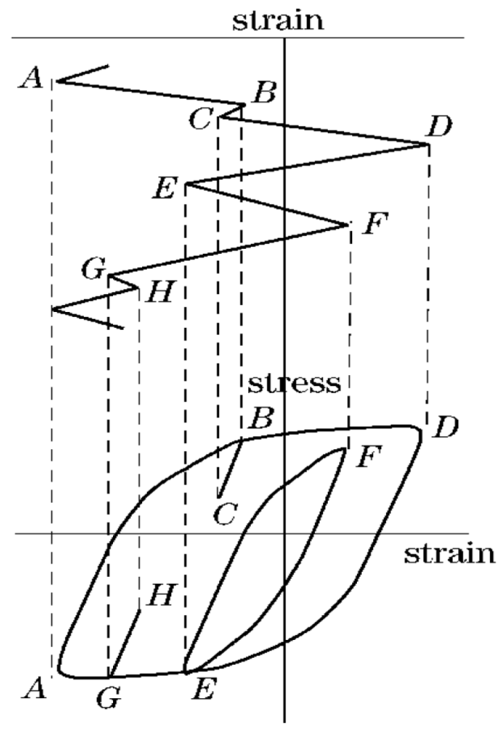
Figure 2.
Cyclic curves of nominal and local stress-strain.
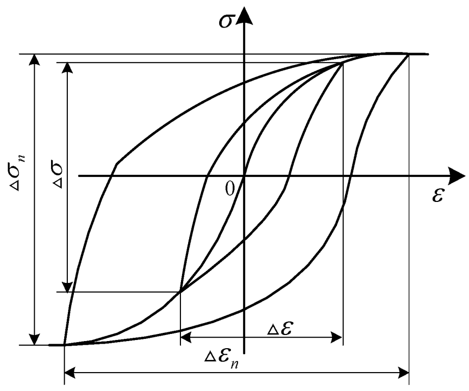
Figure 3.
Morrow mean stress correction model.
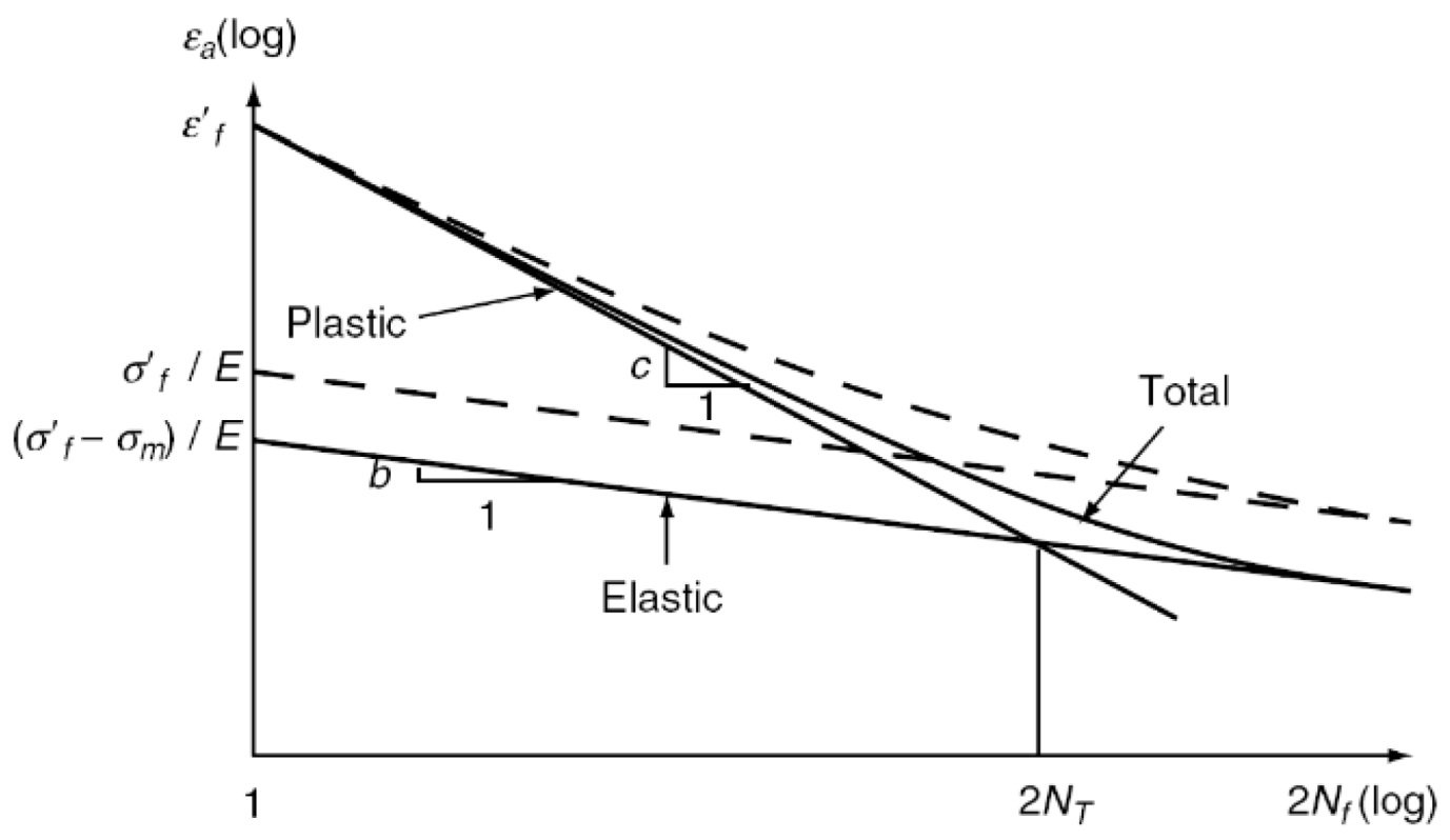
Figure 4.
Vertex coordinates and mean stress of hysteresis loop.
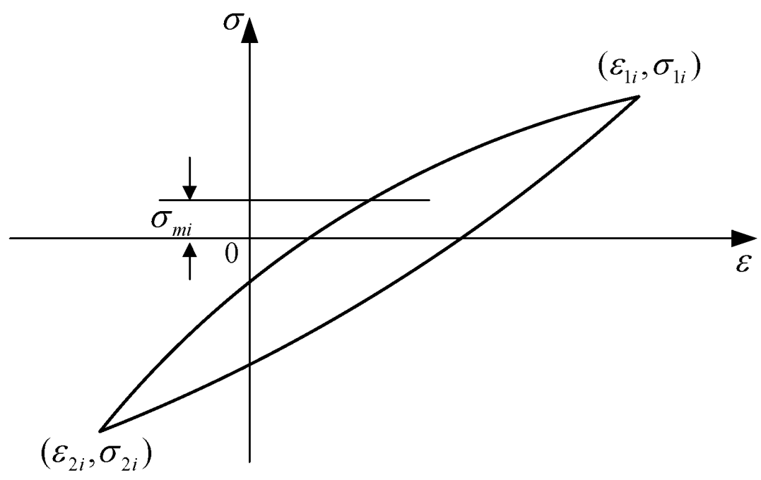
Figure 5.
Strain measurement points on rear axle.
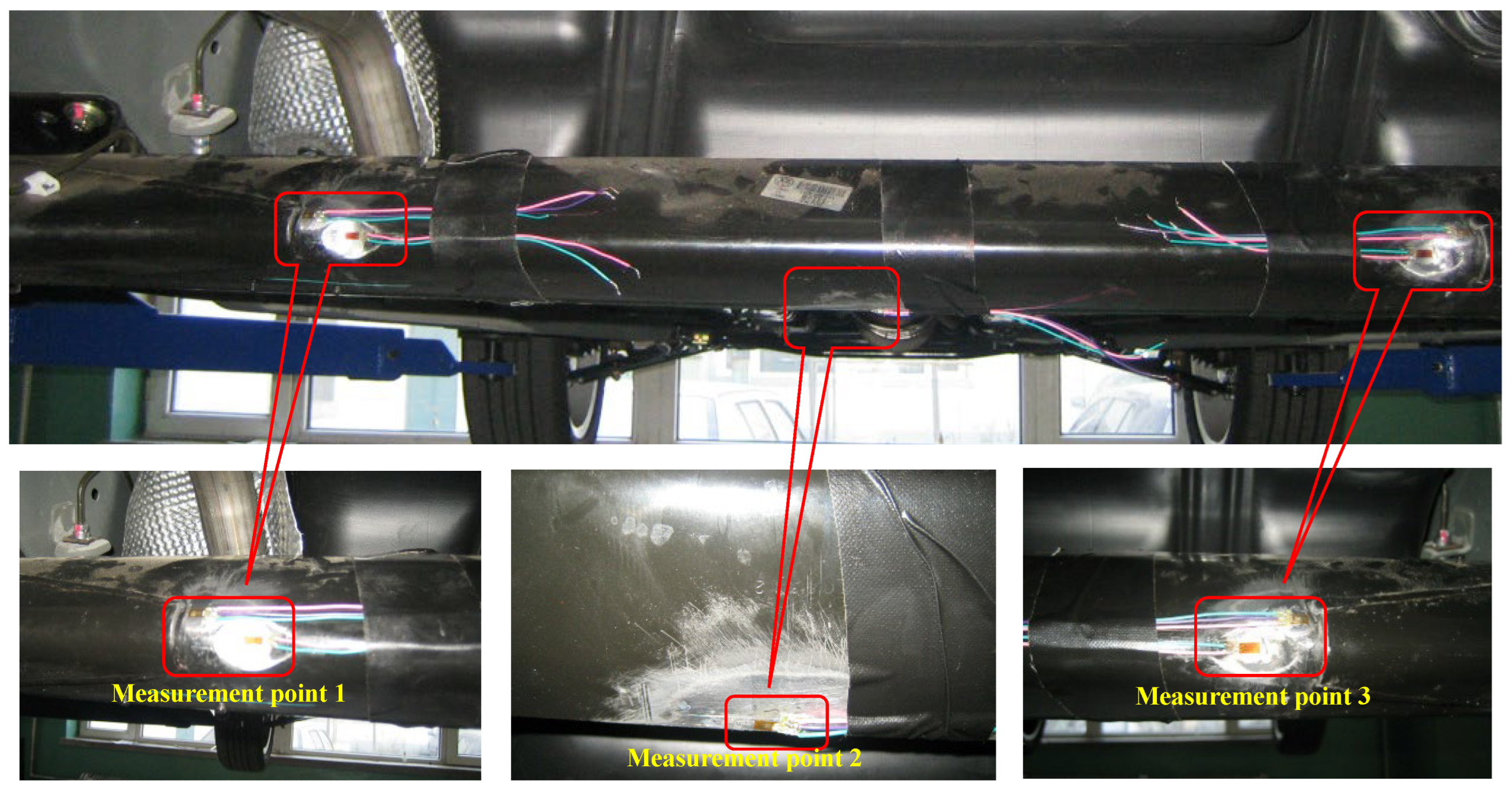
Figure 6.
Acquisition instrument of test data.
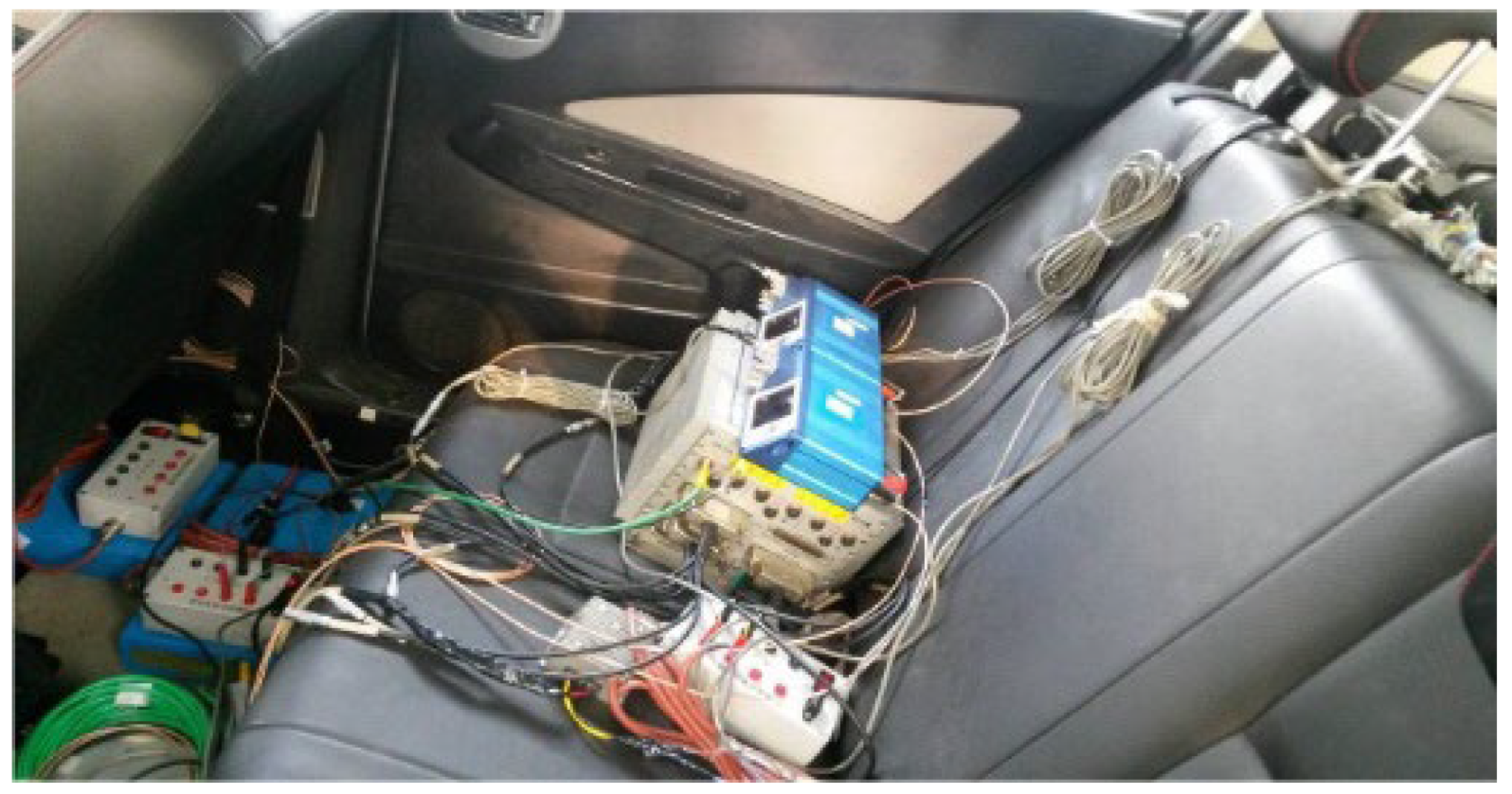
Figure 7.
Real car testing on washboard road.

Figure 8.
Strain time-domain signal of three measurement points on rear axle.
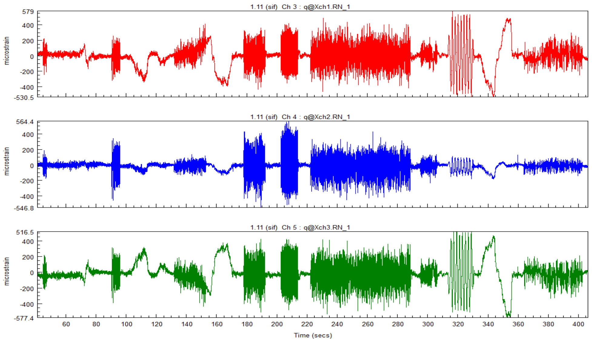
Figure 9.
Acceleration time-domain signals on rear axle end.
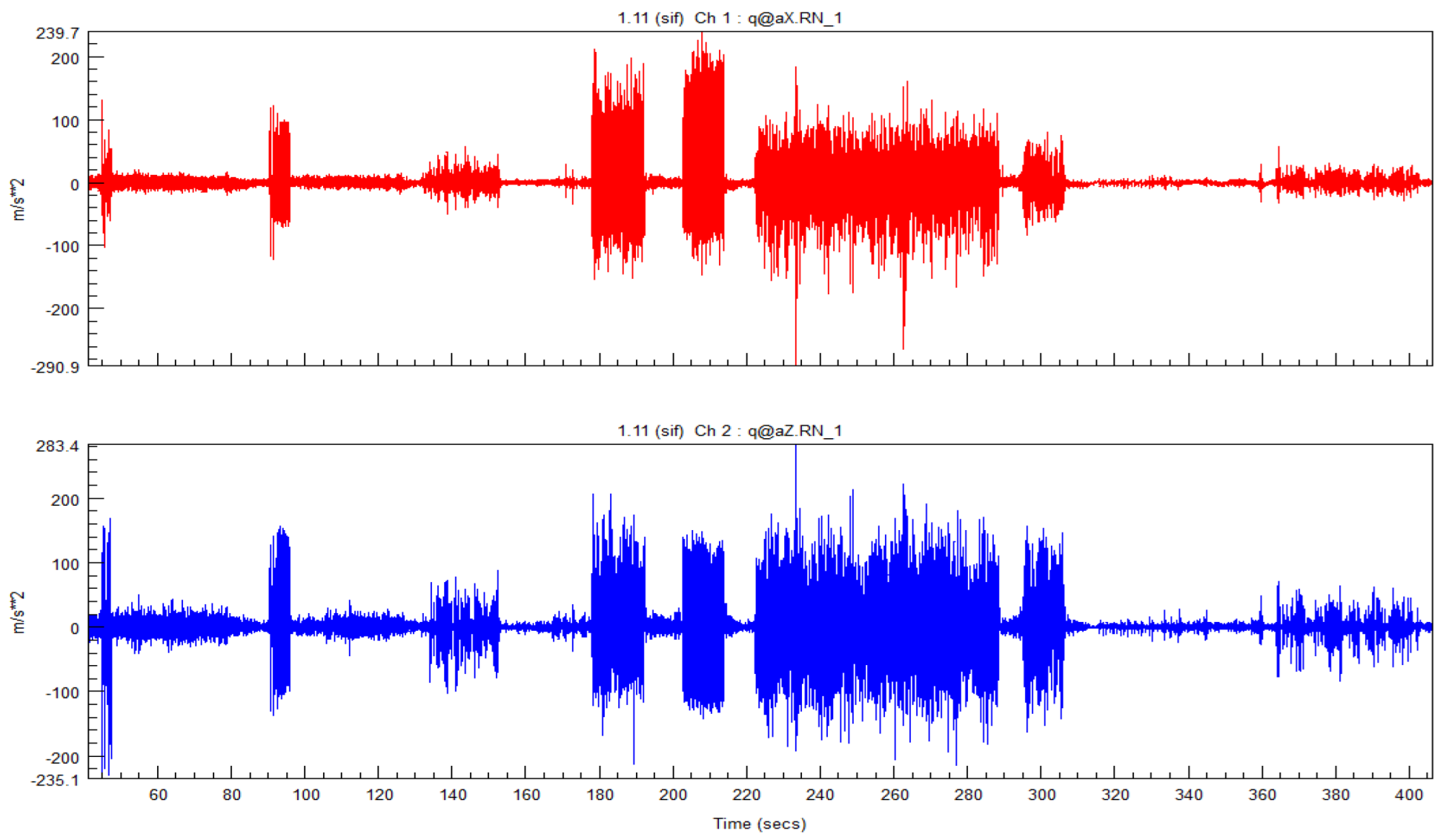
Figure 10.
Test vehicle speed signal.
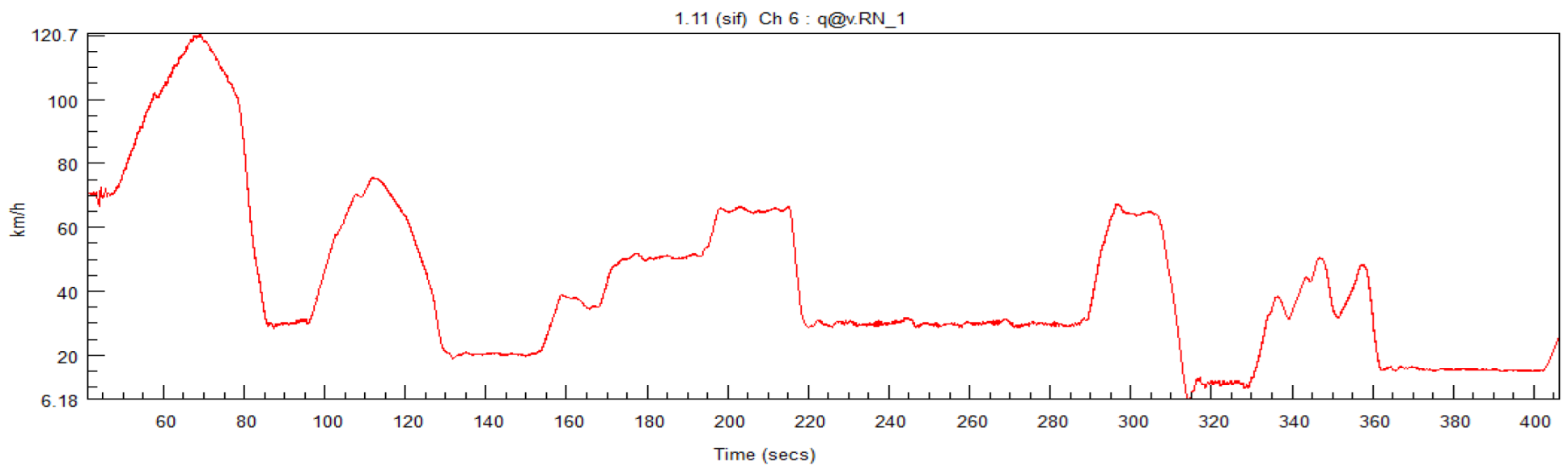
Figure 11.
Stress measurement of rear axle on test rig.
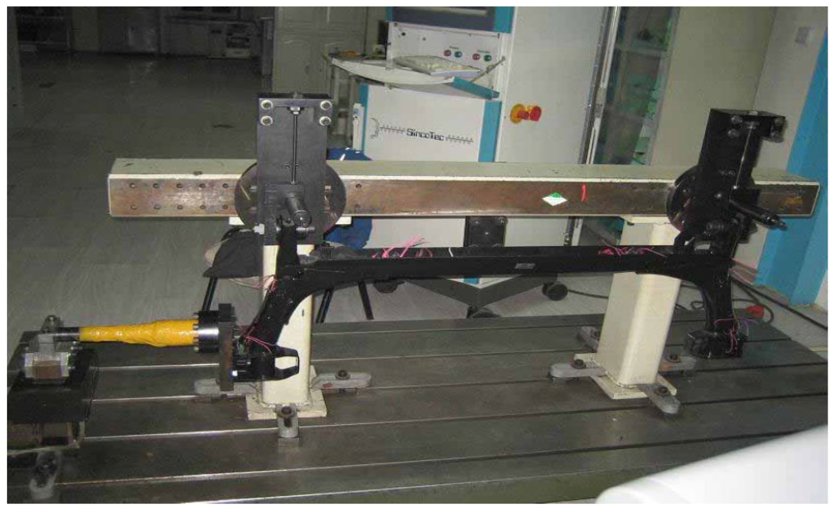
Figure 12.
Preprocessing model of test data based on Glyph Works.
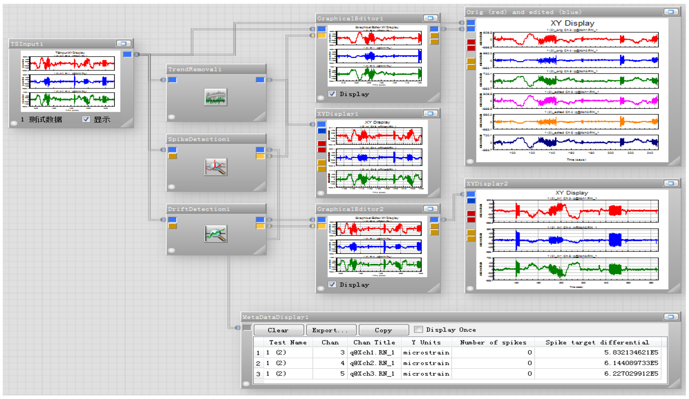
Figure 13.
Fatigue damage calculation model based on Glyph Works.
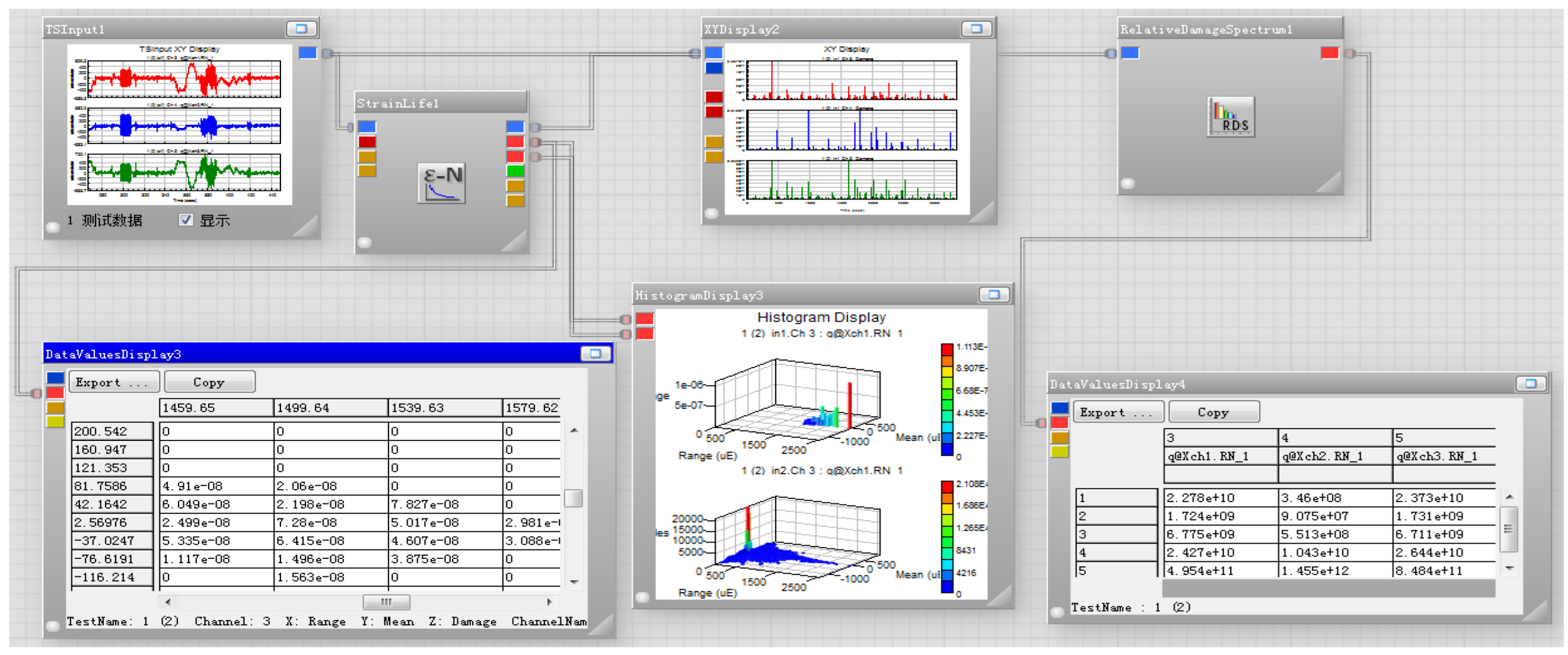
Figure 14.
Accumulated damage comparison of three measurement points.
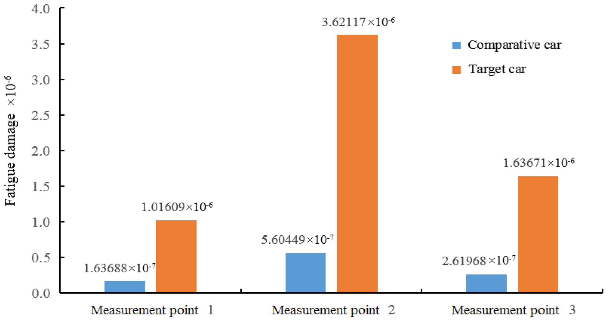
Figure 15.
Damage percentage of measurement point 1 on PG durability road.
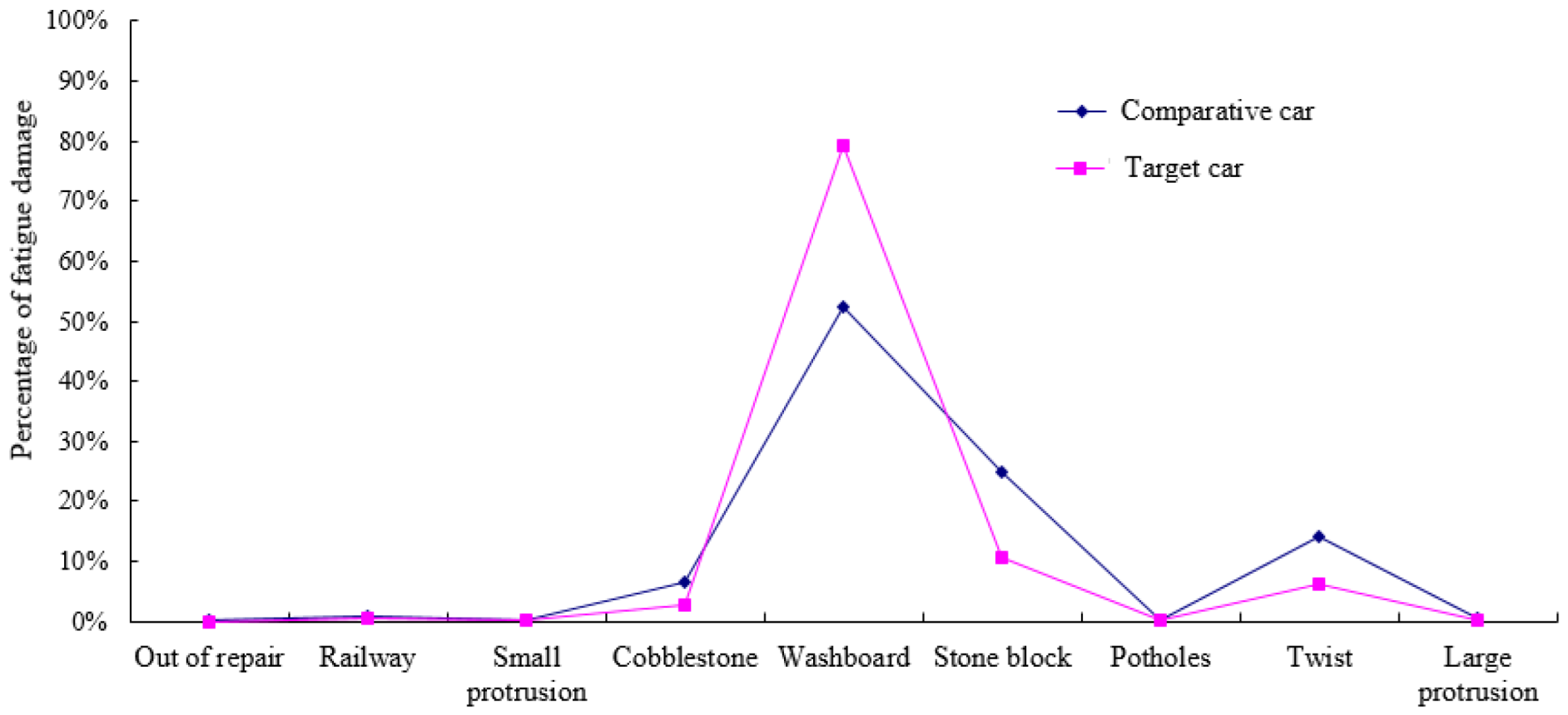
Figure 16.
Damage percentage of measurement point 2 on PG durability road.
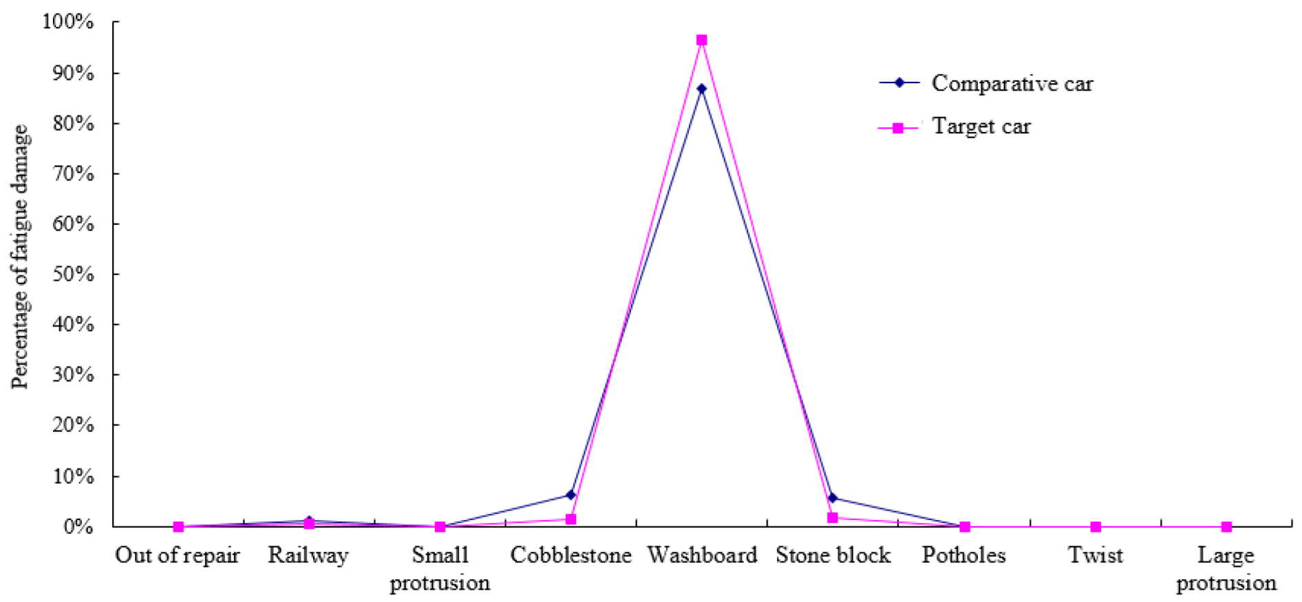
Figure 17.
Damage percentage of measurement point 3 on PG durability road.
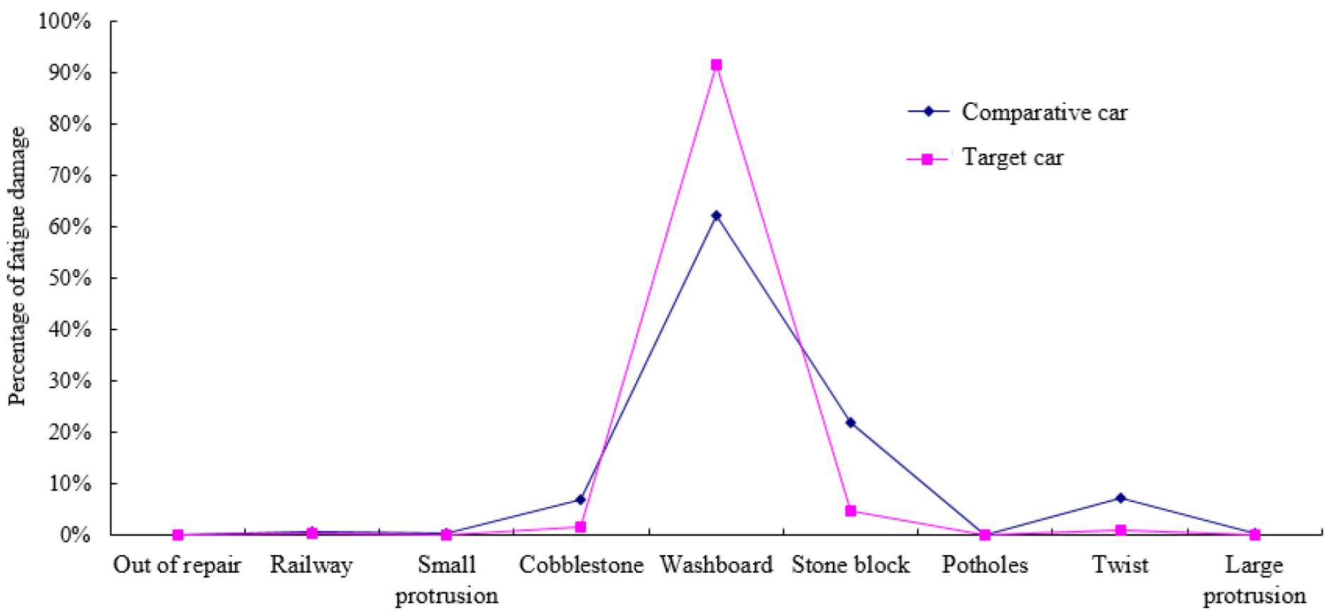
Figure 18.
Cross section of washboard road.
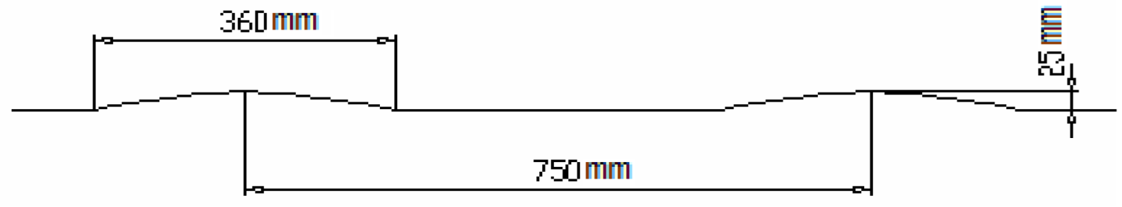
Figure 19.
Generation model of PSD for acceleration responses.
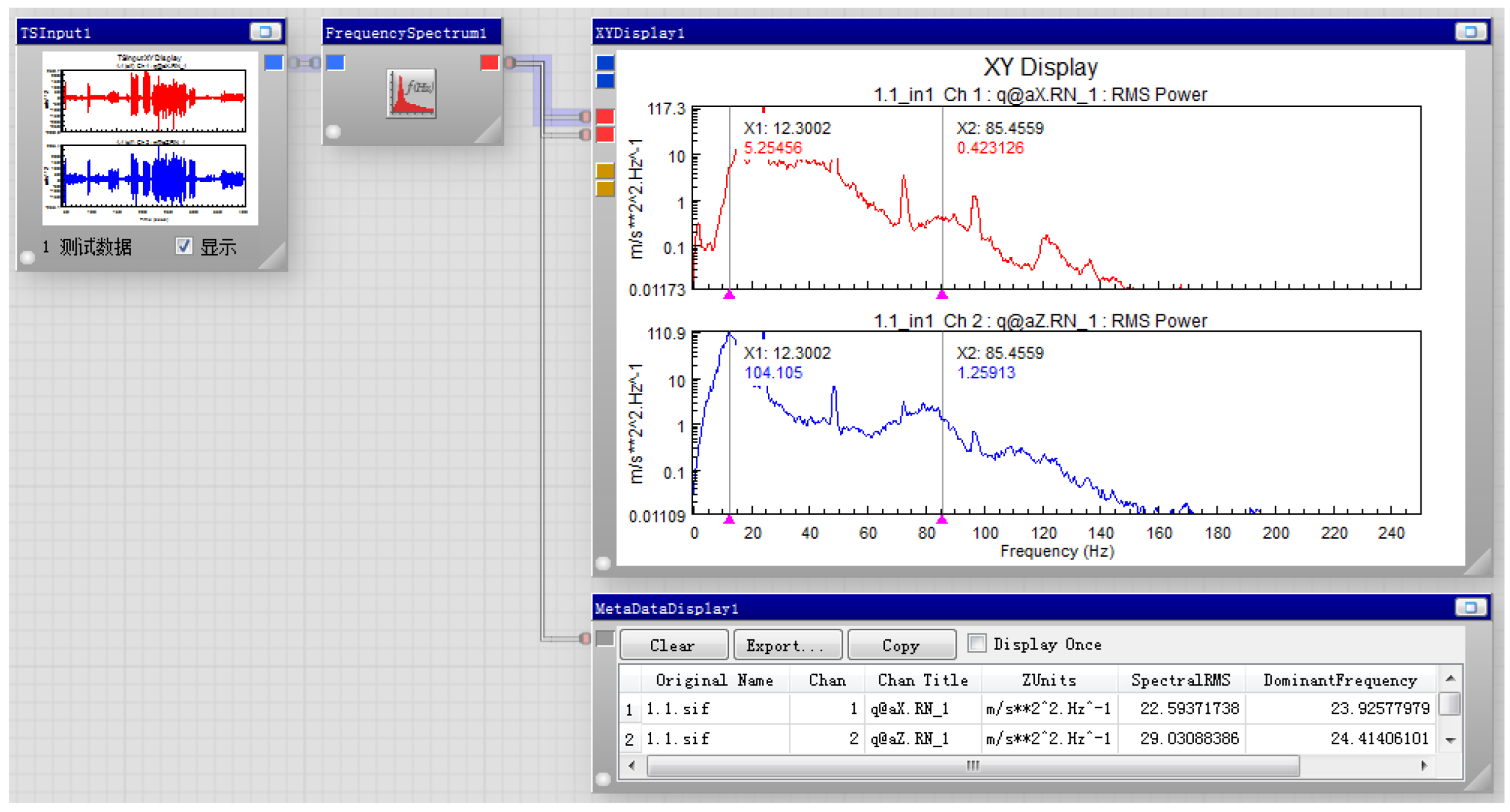
Figure 20.
PSD of acceleration signal of rear axle end on PG durability road.
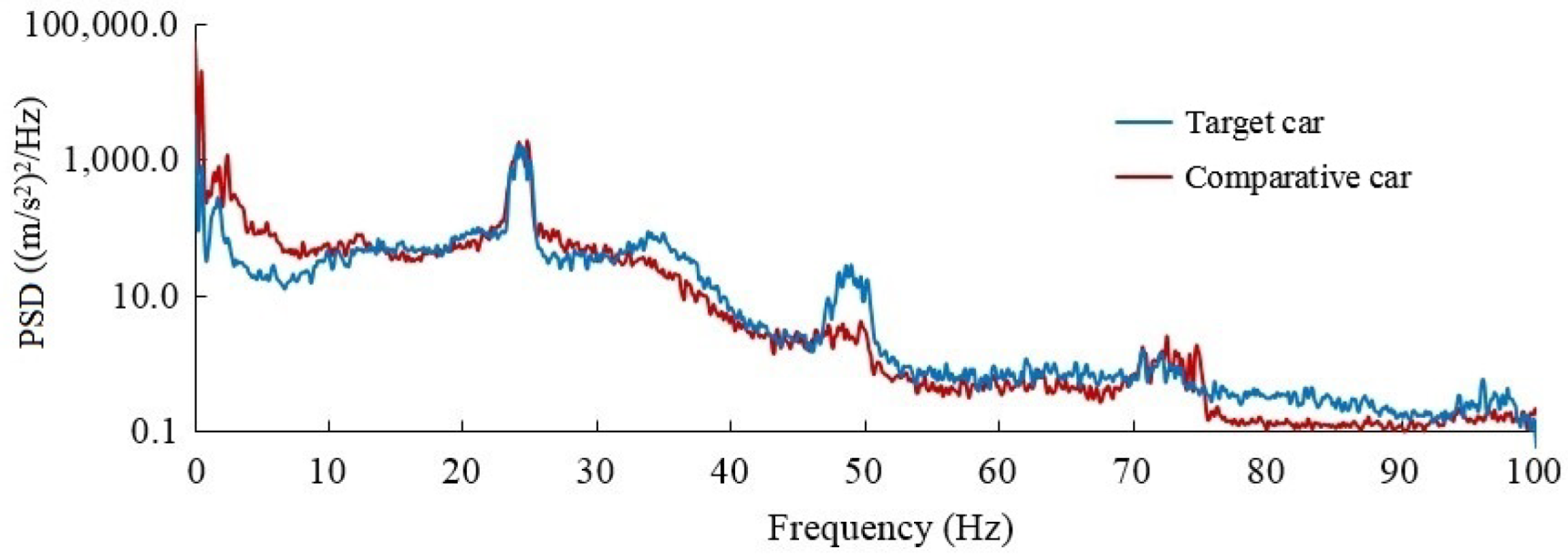
Figure 21.
PSD of acceleration signal of rear axle end on washboard road.
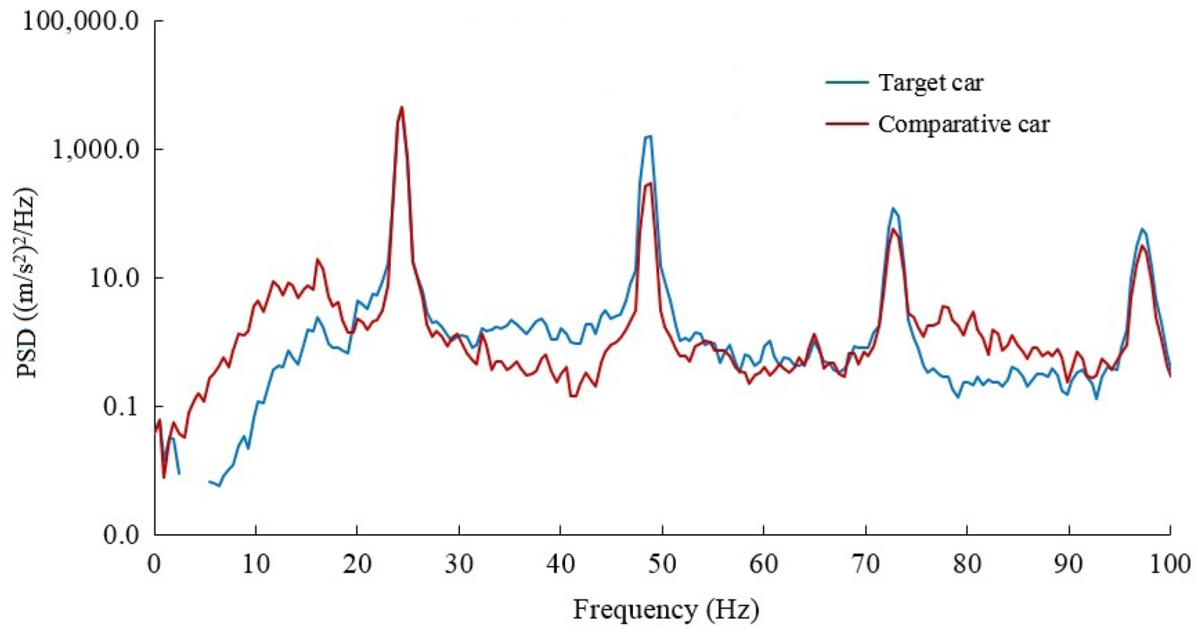
Figure 22.
Damage comparison of measurement point 1 on washboard road.
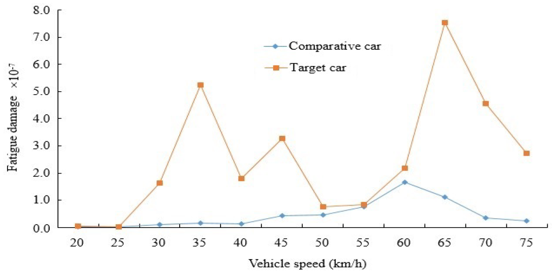
Figure 23.
Damage comparison of measurement point 2 on washboard road.
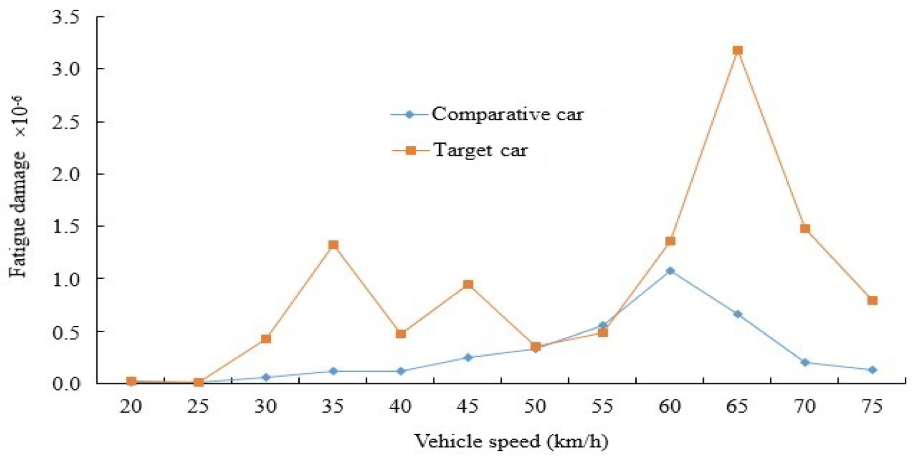
Figure 24.
Damage comparison of measurement point 3 on washboard road.
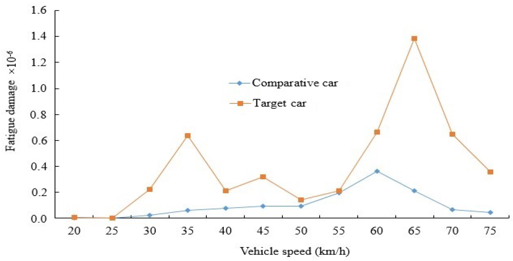
Figure 25.
Modal transfer function curve of target car body.
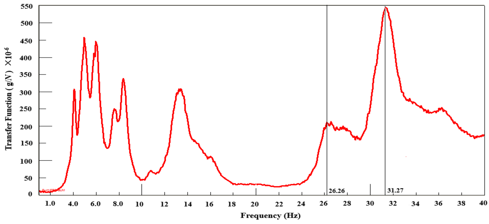
Figure 26.
First-order torsional mode shape of target car body.
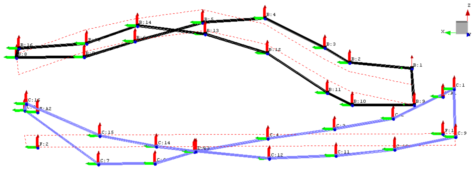
Figure 27.
First-order bending mode shape of target car body.
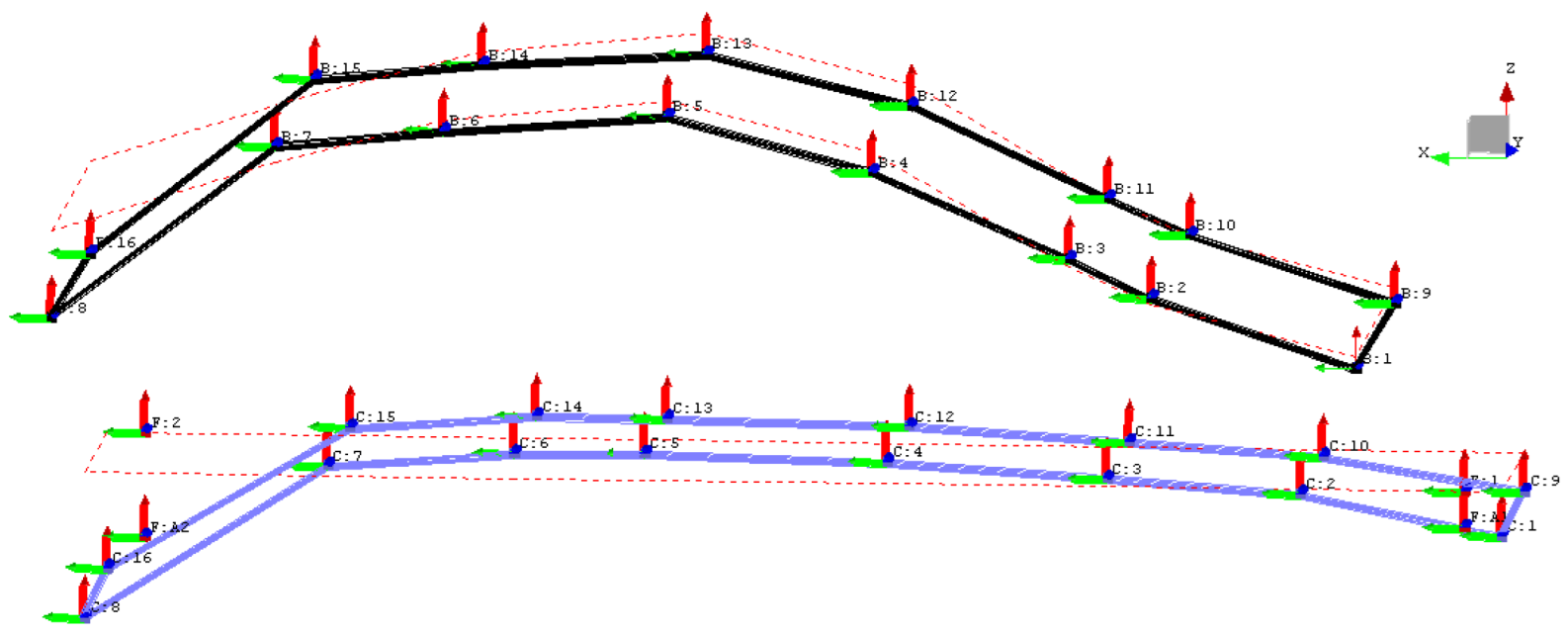
Figure 28.
Modal transfer function curve of rear axle for target car.

Figure 29.
Vertical vibration mode shape of rear axle for target car.
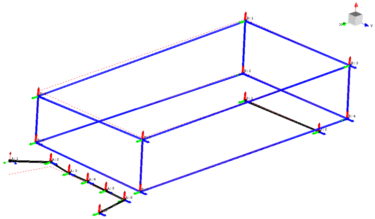
Figure 30.
Modal transfer function curve of comparative car body.
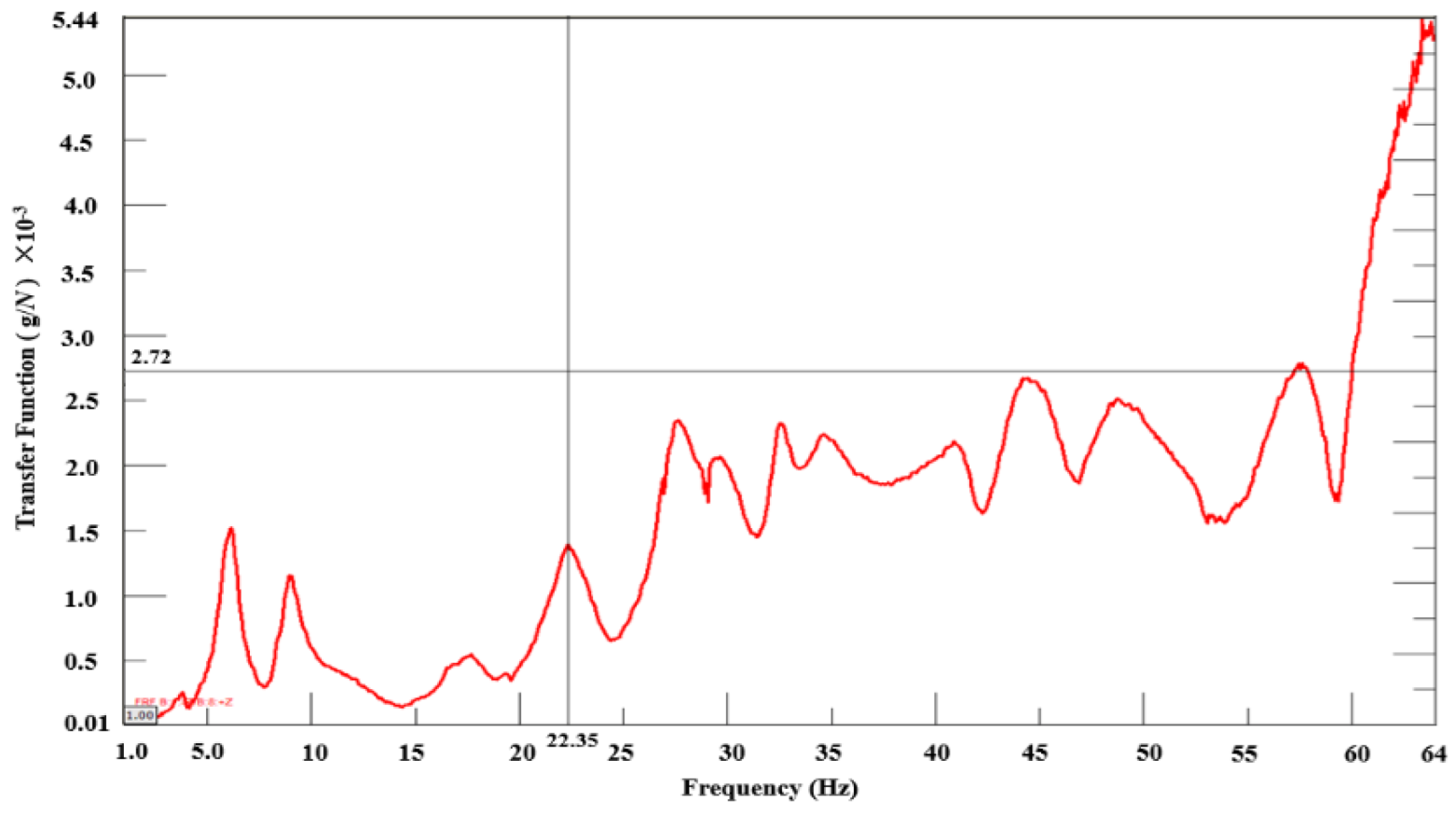
Figure 31.
First-order torsional mode shape of comparative car body.
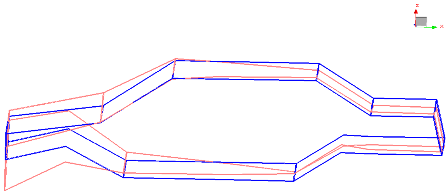
Figure 32.
Modal transfer function curve of rear axle for comparative car.
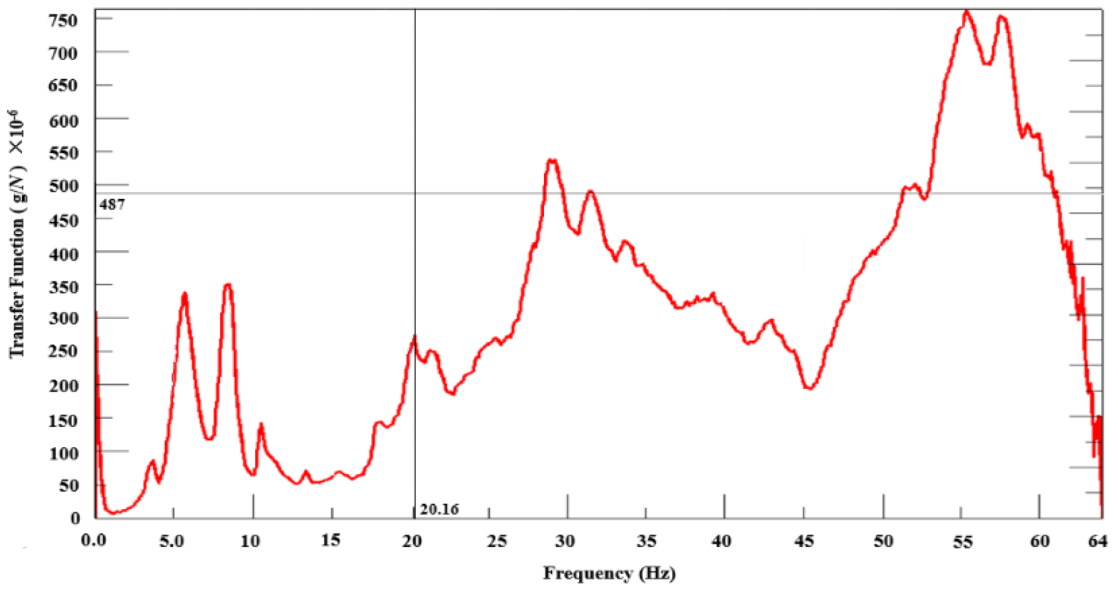
Figure 33.
Vertical vibration mode shape of rear axle for comparative car.
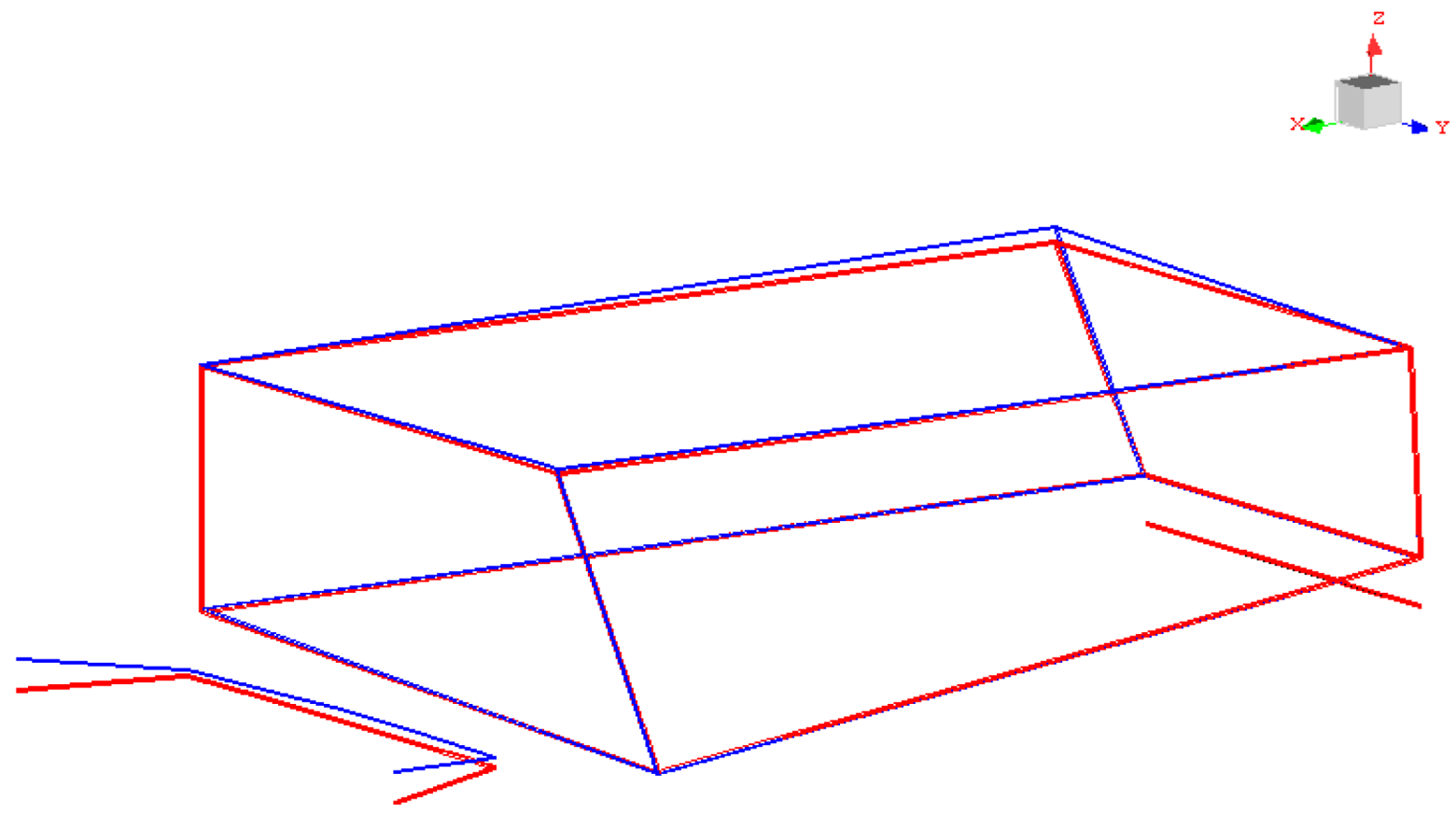

Table 1.
Material parameters of rear axle for damage calculation.
| Parameter | Value |
| Material constant a | 0.046mm |
| Fillet radius of notch root r | 3.50mm |
| Theoretical stress concentration factor Kt | 1.68 |
| Modulus of elasticity E | 2.07×10⁵MPa |
| Poisson’s ratio | 0.3 |
| Cyclic strength coefficient K’ | 2648MPa |
| Cyclic hardening exponent ń | 0.13 |
| Fatigue strength coefficient σ́́f | 1350MPa |
| Fatigue ductility coefficient έf | 0.501 |
| Fatigue strength exponent b | -0.103 |
| Fatigue ductility exponent c | -0.512 |
Table 2.
Maximum test stress at each measurement point.
| Measurement location |
Measurement parameter value (MPa) | Target Car |
Comparative Car | Ratio of target car to comparative car |
| Measurement point 1 | Von Mises stress | 59 | 54 | 1.092 |
| Principal stress 1 | 65 | 62 | 1.048 | |
| Principal stress 2 | -67 | -56 | 1.196 | |
| Measurement point 2 | Von Mises stress | 143 | 131 | 1.092 |
| Principal stress 1 | 160 | 135 | 1.185 | |
| Principal stress 2 | -131 | -122 | 1.073 | |
| Measurement point 3 | Von Mises stress | 69 | 67 | 1.029 |
| Principal stress 1 | 52 | 48 | 1.083 | |
| Principal stress 2 | -56 | -51 | 1.098 |
Table 3.
Damage distribution of three measurement points on PG durability road.
| PG durability road | Comparative Car | Target Car | ||||
| Measurement point 1 | Measurement point 2 | Measurement point 3 | Measurement point 1 | Measurement point 2 | Measurement point 3 | |
| Out of repair | 1.2033×10⁻¹⁰ | 1.1545×10⁻¹⁰ | 1.1690×10⁻¹⁰ | 1.4018×10⁻¹⁰ | 7.2672×10⁻¹¹ | 1.3760×10⁻¹⁰ |
| Railway | 1.2109×10⁻⁹ | 7.2828×10⁻⁹ | 2.5001×10⁻⁹ | 5.4458×10⁻⁹ | 1.6166×10⁻⁸ | 6.6532×10⁻⁹ |
| Small protrusion | 6.1943×10⁻¹⁰ | 5.9324×10⁻¹¹ | 6.9517×10⁻¹⁰ | 1.2863×10⁻⁹ | 1.1871×10⁻¹⁰ | 5.2939×10⁻¹⁰ |
| Cobblestone | 1.0601×10⁻⁸ | 3.5937×10⁻⁸ | 1.7528×10⁻⁸ | 2.9251×10⁻⁸ | 4.8485×10⁻⁸ | 2.7530×10⁻⁸ |
| Washboard | 8.3171×10⁻⁸ | 4.7897×10⁻⁶ | 1.5561×10⁻⁷ | 8.2137×10⁻⁷ | 3.5005×10⁻⁶ | 1.5130×10⁻⁶ |
| Stone block | 4.3704×10⁻⁸ | 3.7872×10⁻⁸ | 6.3032×10⁻⁸ | 9.8639×10⁻⁸ | 5.5360×10⁻⁸ | 7.1334×10⁻⁸ |
| Potholes | 2.9043×10⁻¹⁰ | 1.4872×10⁻¹⁰ | 2.6931×10⁻¹⁰ | 5.9450×10⁻¹⁰ | 2.5382×10⁻¹⁰ | 4.6953×10⁻¹⁰ |
| Twisted | 2.3306×10⁻⁸ | 1.8745×10⁻¹¹ | 2.1340×10⁻⁸ | 5.7418×10⁻⁸ | 8.1182×10⁻¹¹ | 1.6155×10⁻⁸ |
| Large protrusion | 6.6385×10⁻¹⁰ | 4.4213×10⁻¹¹ | 8.6716×10⁻¹⁰ | 1.9363×10⁻⁹ | 7.8974×10⁻¹¹ | 8.0858×10⁻¹⁰ |
Table 4.
Standard deviation of strain signal on washboard road.
| Vehicle speed (km/h) |
Comparative Car | Target Car | ||||
| Measurement point 1 | Measurement point 2 | Measurement point 3 | Measurement point 1 | Measurement point 2 | Measurement point 3 | |
| 20 | 48.16 | 73.02 | 60.32 | 63.95 | 77.13 | 70.88 |
| 25 | 69.51 | 100.28 | 80.61 | 72.10 | 104.60 | 152.89 |
| 30 | 139.04 | 196.10 | 159.05 | 170.63 | 215.79 | 201.26 |
| 35 | 97.34 | 147.29 | 126.93 | 233.62 | 290.50 | 229.97 |
| 40 | 108.64 | 163.95 | 140.20 | 180.15 | 234.51 | 237.60 |
| 45 | 147.49 | 209.30 | 171.89 | 190.96 | 247.70 | 198.58 |
| 50 | 123.30 | 169.14 | 176.95 | 123.20 | 174.47 | 183.89 |
| 55 | 182.02 | 283.49 | 243.71 | 185.41 | 292.20 | 255.64 |
| 60 | 231.83 | 338.91 | 280.78 | 261.84 | 361.94 | 300.16 |
| 65 | 179.96 | 251.78 | 203.76 | 343.17 | 428.30 | 321.08 |
| 70 | 154.07 | 213.22 | 172.99 | 284.53 | 321.45 | 268.65 |
| 75 | 161.20 | 222.24 | 182.95 | 250.49 | 311.40 | 290.73 |
Table 5.
Root mean square (RMS) of acceleration signals on washboard road.
| Vehicle speed (km/h) |
Comparative Car | Target Car | ||
| ax (m/s2) | az (m/s2) | ax (m/s2) | az (m/s2) | |
| 20 | 28.477 | 55.436 | 29.234 | 59.579 |
| 25 | 24.824 | 48.922 | 25.480 | 49.954 |
| 30 | 33.333 | 70.991 | 38.297 | 76.634 |
| 35 | 57.502 | 100.267 | 61.796 | 102.267 |
| 40 | 56.231 | 104.147 | 64.037 | 107.124 |
| 45 | 52.986 | 93.972 | 62.027 | 95.394 |
| 50 | 68.805 | 81.098 | 69.838 | 90.852 |
| 55 | 82.314 | 72.753 | 87.306 | 77.161 |
| 60 | 90.917 | 69.925 | 92.015 | 73.326 |
| 65 | 90.169 | 80.356 | 96.015 | 88.315 |
| 70 | 68.566 | 64.734 | 68.850 | 68.061 |
| 75 | 65.464 | 80.378 | 67.349 | 82.465 |
Table 6.
Frequency sweep results of modal parameters.
| Testing vehicle | Modal type | Natural frequency (Hz) | Damping ratio (%) |
| Target car | First-order torsional mode of car body | 26.26 | 3.76 |
| First-order bending mode of car body | 31.27 | 3.51 | |
| Vertical vibration mode of rear axle | 23.53 | 18.5 | |
| Comparative car | First-order torsional mode of car body | 22.35 | 3.45 |
| First-order bending mode of car body | 27.63 | 3.74 | |
| Vertical vibration mode of rear axle | 20.16 | 5.46 |
Disclaimer/Publisher’s Note: The statements, opinions and data contained in all publications are solely those of the individual author(s) and contributor(s) and not of MDPI and/or the editor(s). MDPI and/or the editor(s) disclaim responsibility for any injury to people or property resulting from any ideas, methods, instructions or products referred to in the content. |
© 2025 by the authors. Licensee MDPI, Basel, Switzerland. This article is an open access article distributed under the terms and conditions of the Creative Commons Attribution (CC BY) license (http://creativecommons.org/licenses/by/4.0/).
Copyright: This open access article is published under a Creative Commons CC BY 4.0 license, which permit the free download, distribution, and reuse, provided that the author and preprint are cited in any reuse.


