
Submitted:
10 April 2025
Posted:
10 April 2025
You are already at the latest version
Abstract
Carpathian Orogen represents a natural laboratory for studying geodynamic interactions between lithospheres of different ages. The ancient Archean Craton, such as the East European Craton, and Proterozoic platforms like the Scythian and Moesian platforms, collided with the younger Tisza and Dacia Mega-Units, resulting in the formation of the current architecture of the Carpathian Mountains. To better understand how lithospheric structure on Romanian territory changes from the East European Craton to younger European microplates, we used earthquake data recorded at permanent broadband seismic stations of the Romanian National Seismic Network (RSN). Applying the Multiple Filtering Technique, we examine the dispersion of Rayleigh wave group velocities for earthquakes located within a 4000 km radius of the epicenter. Travel time tomography, conducted through Fast Marching Surface Tomography, helps us to construct group velocity maps for periods between 30 and 80 s. Our findings highlight a low velocity body in front of the Vrancea slab, indicating asthenospheric upwelling due to slab verticalization.
Keywords:
Rayleigh wave
; group velocity tomography
; Vrancea slab
; multiple filter technique
; asthenospheric upwelling
1. Introduction
The present-day Carpathians configuration (Figure 1) is evidence of plate convergence process that began in the Late Cretaceous and continued through the Tertiary and Quaternary [1]. The tectonic units of the Carpathian orogen are part of the Alpine-Carpathian-Dinaric orogenic system with a complex geometry and tectonic evolution. In the Late Jurassic (ca. 156 Ma), the new Alpine Tethys opened, and its branches led to the separation of the ALCAPA (Alpine-Carpathian Pannonian), Tisa, and Dacia mega-units from the European continent. The Ceahlau-Severin Ocean in the Eastern Carpathians is a distinct segment of the Alpine Tethys that stretches towards the east but does not connect to the ancient Meliata-Maliac Ocean crust, which dates back to the Triassic period [2].
The compressional regime began in the Cretaceous and led to the closure of these ancient oceans and the consumption of oceanic lithosphere and thinned continental lithosphere. In the later stages of this compressional process, the formation of fold-thrust belts and the emergence of Neogene volcanism occurred [3]. The Neogene-Quaternary magmatism associated with the subduction process along the Carpathian orogen displays unique features within the inner part of the Carpathian Curvature. The observed characteristics indicate a shift in the composition and structure of the lithosphere, which has significant implications for the geodynamic process of subduction in this region [4]. The utilization of surface wave seismic tomography proves to be a valuable approach in unraveling the intricate tectonic evolution of the Carpathian orogen.
The study of Rayleigh wave propagation in orogenic belts is an important technique for understanding the structure and evolution of mountain belts. Surface waves are long-period waves often used to image seismic velocities in the crust and upper mantle [5,6,7,8]. Surface wave models are based on dispersion properties of Rayleigh and Love waves and are the best indirect imaging tools available to accurately estimate absolute velocities at depth
Several tomographic studies were carried out in our study area, most of them focused on the Vrancea seismic zone. Tomographic studies have been conducted using body wave data [9], both body wave and S wave data [10], as well as full-wave tomography [11]. However, as opposed to surface waves, body wave-tomography offers relative travel-time information with poor vertical resolution.
Seismic tomography is very useful for visualizing the actual tectonic configuration at depth, providing valuable information about the geodynamic evolution of the Carpathian orogen.
In other studies, like core-refracted shear wave anisotropy (SKS), [12] pointed out that anisotropy aligning with the upper slab is initially perpendicular but then switches to a parallel orientation, indicating the recent retreat and rollback of the slab. The mechanics of intermediate-depth earthquakes do not follow the classic crustal earthquake mechanism and could be accompanied by additional processes. Brittle failure at high depth is likely associated with ductile deformation [13].
A striking decrease in stress ratio with increasing earthquake magnitude [14] shows that small earthquakes are dominantly thrust-fault types associated with vertical elongation. For larger earthquake generation, mineralogical phase changes or dehydration embrittlement mechanisms were suggested [14,15]
2. Data and Methods
2.1. Earthquake Data and Seismic Stations
In this study, we analyzed the dispersion of Rayleigh waves generated by earthquakes with epicentral distances less than 40 degrees (around 4000 km) and magnitude Mb greater than 4.5. Data came recorded by 23 broadband stations of the Romanian Seismic Network (RSN) between 2011 and 2018. The waveforms were truncated by 3000 s after the origin time of the earthquake to ensure the capture of the events depicted in Figure 1. To reduce the file size and boost the data processing, the waveforms were decimated at a sampling rate of 0.5 s, which does not affect the signal generated by our target surface waves, whose periods range between 15 and 150 s. The earthquakes that generated high-quality surface waves from which dispersion could be extracted are represented in Figure 2. Seismic sources originate in the Mediterranean Sea region and Iran predominantly, as well as in the North Atlantic region. The intersection of these rays is essential for high-resolution tomography without numerical artifacts caused by lack of coverage.
2.2. Rayleigh Wave Dispersion
Obtaining accurate measurements of group velocities or phase velocities of surface waves, such as Rayleigh waves, is a crucial tool for surface wave tomography. Given the non-homogeneous nature of Earth's lithosphere, the dispersion of surface waves plays a substantial role. This is because the velocities of these waves vary depending on the depth range sampled at each frequency/period. To analyse Rayleigh wave group velocity dispersion, we used the Computer Codes for Seismology software (CPS) [16]. We applied the Multiple Filter Technique (MFT) to isolate group velocities as a function of time. Data processing involves applying multiple filters to the seismogram and enables interactive data visualization, allowing the user to select the maximum amplitude for each frequency/period of the fundamental mode of Rayleigh or Love waves. The method uses a Gaussian filter (Hω) described by eq. 1 to filter the dispersed signal mode of surface-wave expressed by eq. 2. In eq.1 α represents a resolution testing parameter, ω0 represents the central frequency (peak of Gaussian function), ωn is a parameter that determines the width of the function. Eq. 2 illustrates the dispersion of a surface wave, with ϴ representing the phase of the source, k representing the wave number, and r representing the distance of the seismic signal.
The choice of the filtering parameter α is important and should be selected based on the epicentral distances of seismic sources, with higher values of α for seismic events with greater epicentral distances. Since the maximum epicentral distance was below 4000 km, α was set to be less than 100s.
The extraction of fundamental mode dispersion curves was done interactively, by selecting peak amplitudes of the signal at discrete periods. Figure 3 shows an example of the interactive CPS program output for the recovery of Rayleigh wave group velocities.
2.3. Seismic Tomography: The Fast-Marching Method
To map the distribution of group velocities across the Carpathian Orogen, we used the Fast Marching Surface Tomography (FMST) method [17]. FMST performs a travel time tomography using an iterative non-linear inversion in spherical coordinates. The arrival times of surface waves were calculated initially using a fast-marching algorithm, where a data gridding method is used to solve the eikonal equations governing wave propagation. For solving the inverse problem, a gradient-based method is employed that iteratively minimizes an objective function containing a residual data term and two regularization terms (ɛ, η). At each iteration, the model is perturbed and updated according to Equation (3):
where A represents the subspace matrix, G is the matrix of group arrival time gradients from the model m, Cm is the covariance matrix of the a priori model, D is a damping operator, and represents the difference between the observed and synthetic data at the current iteration. The damping factor serves the purpose of restricting the deviation of the solution model from the initial model, effectively keeping it within a reasonable range, while the smoothing factor constrains the smoothness of the solution model. An optimum combination of damping and smoothing is essential for estimating a model that compromises between data fit and seismic model variance, offering realistic velocity anomalies. For our inversion, the damping and smoothing parameters were set to 30 and 100, respectively. The model was parametrised on a 0.2°x0.2° grid with velocity nodes in spherical shell coordinates.
To map the distribution of group velocities on the gridded model, we first computed initial travel time values between source and receiver locations based on estimated dispersion curves at each period. The travel time field was estimated using the fast-marching method, by forward modelling the eikonal equation on the gridded model. This initial model served as input for the subsequent iterative inversion that accounts for ray-bending [17]. Velocities in each grid cell and ray paths were then adjusted iteratively using the fast-marching method and a subspace inversion scheme that satisfies the observed data and regularization constraints [18].
3. Results and Discussion
Using the Multiple Filter Technique, we obtained 396 Rayleigh wave group velocity dispersion curves with a period range of 5s to 160s (Figure 4) from earthquakes with epicentral distances ranging from 568 km to 3327 km. The coverage with Love waves was not sufficient for preliminary tomography and requires data processing over a longer period of time, encompassing earthquakes with higher signal-to-noise ratios.
In Figure 4, the dispersion curves estimated at the VLDR seismic station are presented, color-coded based on the earthquake azimuth. We observed higher group velocities for earthquakes originating from the southwest of Europe (yellow lines) compared to the group velocities from earthquakes in the south-southeast direction (orange lines).
In the upper mantle, minerals like olivine have a tendency to align themselves in the same direction as the applied stress, and preferential orientation leads to an anisotropic behaviour in the propagation of surface waves [19,20]. At lower depths, a similar phenomenon occurs, where Feldspar, being the most abundant mineral in the Earth's crust, maintains it’s brittle behaviour. Meanwhile, quartz and mica exhibit plastic deformation primarily through dislocation creep, resulting in the development of feldspar microboudinage [21]. According to the European active tectonic strain-stress map shown by [22], the higher group velocities for the seismic sources produced in the Mediterranean Sea (south-west) could be caused by the crystallographic preferred orientation.
Data from Rayleigh wave group velocity dispersion curves were then integrated in the FMST tomography routine which converged successfully (Figure 5A) to construct group velocity maps at discrete periods between 30 and 80 s (Figure 6). Residual travel times shown in Figure 5A are distributed around zero, indicating a good convergence of the inversion.
The correspondence between period and the depth-interval to which surface waves are sensitive is not straightforward and changes with depth and the considered seismic velocity model. Using the local seismic model [23], we forward-modeled the sensitivity kernels for Rayleigh wave group velocities which helped us interpret the frequency-dependent maps. Figure 5B shows that surface wave depth sensitivity decreases inversely with the period. The sensitivity depth interval also widens as the wave period increases, leading to a greater uncertainty in estimating heterogeneities at greater depths.
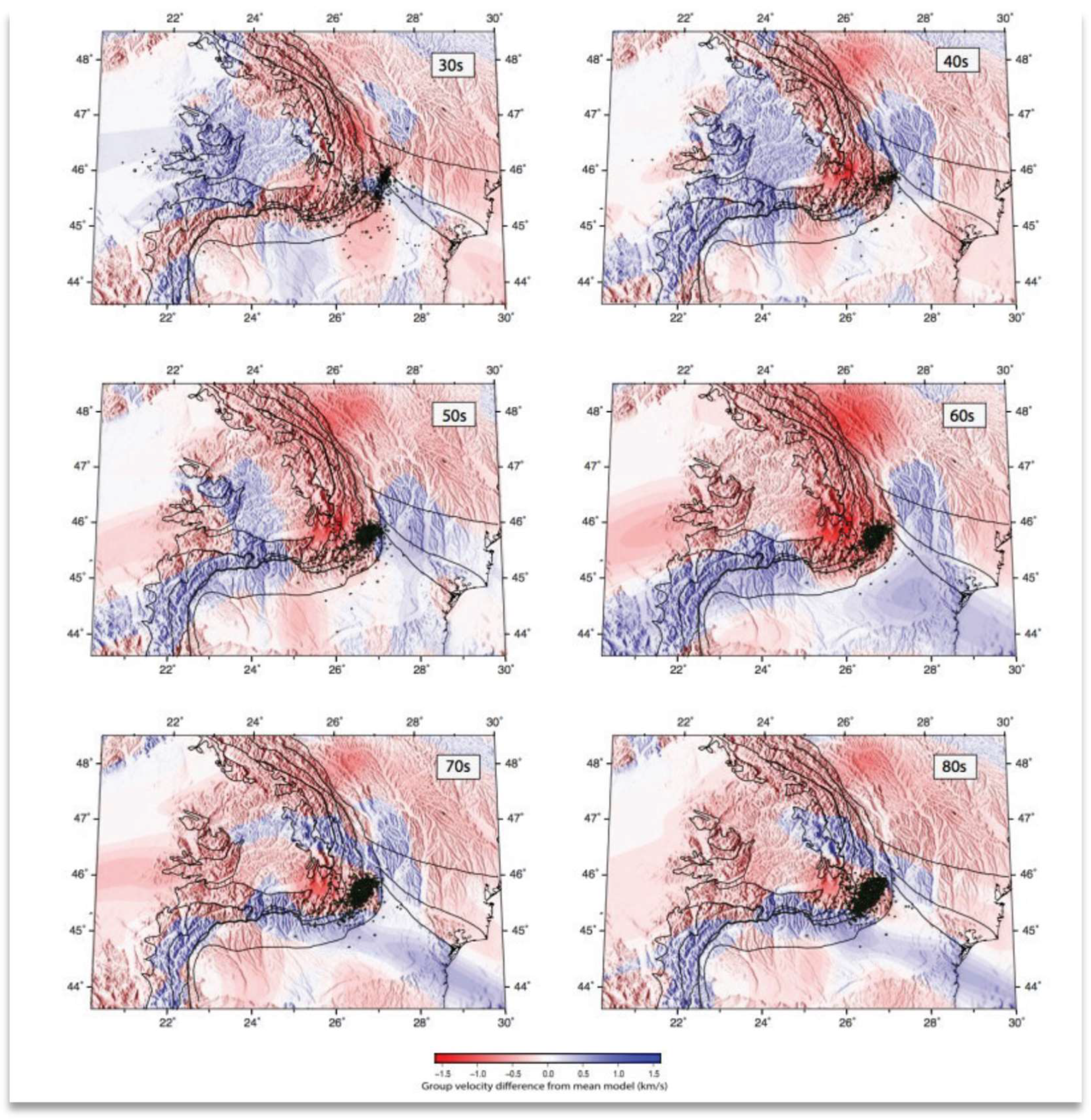
At low periods (30 s), group-velocity maps show slow seismic velocities consistent with over-thrusted Carpathian folds which are mostly formed by rocks poorly consolidated. The Rayleigh waves with a period of 50 s propagate through an interval of 50-80 km (Figure 5B). The group velocity maps generated from these dispersions highlight the Scythian Platform, and parts of Moesia and the EEC as regions characterized by high velocities.
The platform units or Craton-type units are characterized by greater thickness, older age, and faster seismic wave travel. The map generated using the dispersions with 60-second periods best highlights the separation of platform-type units located outside the Carpathian arc from the younger and slow-seismic units located above the Transylvanian and the Pannonian basins. Additionally, on the same period, we observe an artifact in the northeastern part, generated by the inversion model due to the lack of ray paths intersections in that area. This lack is primarily due to the absence of seismic sources in the northeastern part of the study area and not by a weak distribution of receivers/broadband seismic stations.
Group velocity maps starting with 40s period indicate the presence of a region with reduced group velocities located in front of the Vrancea lithospheric slab (adjacent to the seismogenic body to the NW), which suggests the possibility of an asthenospheric upwelling cell, which has been previously suggested [24,25]. In the context of collisional processes, these upwelling cells can be observed in subduction zones where two tectonic plates converge, and one plate is forced beneath the other. As the denser oceanic lithosphere sinks into the underlying mantle, it exerts a downward force on the overriding plate.
This process can also impact the behaviour of the asthenosphere, potentially leading to the development of asthenospheric upwelling cells [26]. The change in the volcanism's composition in front of the Vrancea seismic zone, as well its propagation direction, has been attributed to a toroidal flow of the asthenosphere accompanying the gradual subduction of the Vrancea lithospheric fragment [4].
We obtained maps of Rayleigh wave dispersion curves at different periods: 30 s, 40 s, 50 s, 60 s, 70 s, and 80 s. The anomaly is most visible on the 40 s and 50 s and 60s period maps, which correspond to a depth range of 50–90 km.
4. Conclusions
This In this study, we analyzed the group velocity dispersion of Rayleigh waves generated by regional earthquakes with an epicentral distance of less than 40 degrees (about 4000 km) and a magnitude Mb> 4.5. The data studied consist of records from 23 RSN broadband stations covering the period between 2011 and 2018. We further used the fast-marching method and an iterative subspace inversion scheme to construct frequency-dependent maps of Rayleigh wave group velocities across the Carpathian Orogen.
Our new results confirm the presence of slow velocities in the overthrusting Carpathian folds at low periods (30s). For periods longer than 50s, group velocity maps show locally high seismic velocity amplitudes in the East European Craton, the Scythian, and the Moesian platforms.
We observed an asthenospheric upwelling occurring in front of the Vrancea slab, which is generated by the sinking of the slab. The analysis of Rayleigh wave group velocities indicated that this low-velocity region is located at a depth range of 50-90 km.
Author Contributions
Conceptualization, A.M., L.P. and I-A.M; methodology, A.M., L.P and M.R; software, L.P, A.M; validation, A.M., L.P., M.R. and I-A. M; formal analysis, A.M., L.P and M.R; investigation, A.M., L.P; resources, L.P., A.M, M.R. and I-A. M. ; data curation, A.M. and L.P.; writing—original draft preparation, A.M. L.P. and I-A. M.; writing—review and editing, M.R., L.P., A.M., and I-A. M.; visualization, A.M., L.P., M.R and I-A. M.; supervision, X.X.; All authors have read and agreed to the published version of the manuscript.
Funding
The present study was funded by the Nucleu Program SOL4RISC PN23360201.
Data Availability Statement
Dataset available on request from the authors.
Acknowledgments
The present study was funded by the Nucleu Program SOL4RISC. We would like to thank the EENSANE (East European Ambient Seismic Noise) Project PN-III-P4-ID-PCE-2020-2972, supported by UEFISCDI (Executive Agency for Higher Education, Research, Development, and Innovation Funding), Romania, and by MCI, project no. PN23360201. Most figures were created using the Generic Mapping Tools (GMT) (Wessel & Smith, 1998).
Conflicts of Interest
The authors declare no conflicts of interest.
Abbreviations
The following abbreviations are used in this manuscript:
| RSN | Romanian National Seismic Network |
| ALCAPA | Alpine-Carpathian Pannonian |
| SKS | Core-refracted shear wave anisotropy |
| CPS | Computer Codes for Seismology software |
| MFT | Multiple Filter Technique |
| FMST | Fast Marching Surface Tomography |
| EEC | East European Craton |
References
- Csontos, L,; Vörös, A., Mesozoic plate tectonic reconstruction of the Carpathian region. Palaeogeography, Palaeoclimatology, Palaeoecology 2004, 210.1:1-56. [CrossRef]
- Schmid, S.M.; Bernoulli, D.; Fügenschuh, B.; Matenco, L.; Schefer, S.; Schuster, R.; Tischler, M.; Ustaszewski, K. The Alpine-Carpathian-Dinaridic orogenic system: correlation and evolution of tectonic units. Swiss Journal of Geosciences 2008, 101, pp.139-183.
- Mason, P. R.; Seghedi, I.; Szákacs, A.; Downes, H. Magmatic constraints on geodynamic models of subduction in the East Carpathians, Romania. Tectonophysics 1998, 297(1-4), 157-176. [CrossRef]
- Seghedi, I.; Maţenco, L.; Downes, H.; Mason, P. R.; Szakács, A.; Pécskay, Z. Tectonic significance of changes in post-subduction Pliocene–Quaternary magmatism in the south east part of the Carpathian–Pannonian Region. Tectonophysics 2011, 502(1-2), 146-157. [CrossRef]
- Schivardi, R.; Morelli, A. Surface wave tomography in the european and mediterranean region. Geophysical Journal International 2009, 177(3), 1050–1066. [CrossRef]
- Shan, B.; Xiong, X.; Zhao, K.; Xie, Z.; Zheng, Y.; Zhou, L. Crustal and uppermantle structure of south china from rayleigh wave tomography. Geophysical Journal International 2017, 208(3), 1643–1654. [CrossRef]
- Chen, Y., Badal, J., Hu, J., 2010. Love and rayleigh wave tomography of the qinghaitibet plateau and surrounding areas. Pure and Applied Geophysics 167, 1171–1203. [CrossRef]
- Petrescu, L.; Darbyshire, F.; Bastow, I.; Totten, E.; Gilligan, A. Seismic anisotropy of precambrian lithosphere: Insights from rayleigh wave tomography of the eastern superior craton. Journal of Geophysical Research: Solid Earth 2017, 122(5), 3754–3775. [CrossRef]
- Martin, M.; Wenzel, F.; Group, C.W. High-resolution teleseismic body wave tomography beneath se-romania-ii. imaging of a slab detachment scenario. Geophysical Journal International 2006, 164(3), 579–595. [CrossRef]
- Zaharia, B.; Enescu, B.; Radulian, M.; Popa, M.; Koulakov, I.; Parolai, S., , Determination of the lithospheric structure from carpathians arc bend using local data. Romanian Reports in Physics 2009, 61(4), 748–764.
- Baron, J.; Morelli, A. Full-waveform seismic tomography of the vrancea, romania, subduction region. Physics of the Earth and Planetary Interiors 2017, 273, 36–49. [CrossRef]
- Petrescu, L.; Mihai, A.; Borleanu, F.. Slab tear and rotation imaged with core-refracted shear wave anisotropy. Journal of Geodynamics 2023, 157, p.101985. [CrossRef]
- Braeck S.; Podladchikov Y.Y.; Medvedev S. Spontaneous dissipation of elastic energy by selflocalizing thermal runaway, Physical Review 2009, E 80 (4), 046105. [CrossRef]
- Petrescu, L.; Borleanu, F.; Radulian, M.; Ismail-Zadeh, A.; Maţenco. Tectonic regimes and stress patterns in the Vrancea Seismic Zone: Insights into intermediate-depth earthquake nests in locked collisional settings, Tectonophysics 2021, 799, p.228688. [CrossRef]
- Mihai, A.; Moldovan, I. A.; Toader, V. E.; Radulian, M.; Placinta, A. O. Correlations between geomagnetic anomalies recorded at Muntele Rosu seismic Observatory (Romania) and seismicity of Vrancea zone. Rom. Rep. Phys 2019, 71(3), 714.
- Herrmann, R.B. Computer programs in seismology: An evolving tool for instruction and research. Seismological Research Letters 2013, 84(6), 1081–1088. [CrossRef]
- Rawlinson, N.; Sambridge, M. The fast marching method: an effective tool for tomographic imaging and tracking multiple phases in complex layered media. Exploration Geophysics 2005, 36(4), 341–350,.
- Rawlinson, N.; Sambridge, M. Seismic traveltime tomography of the crust and lithosphere. Advances in geophysics 2003, 46, pp.81-199.
- Cara, M.; Leveque, J. Oriented olivine crystals in the upper mantle: a test from the inversion of multimode surface-wave data. Physics of the earth and planetary interiors 1987 ,47, 246–252. [CrossRef]
- Mainprice, D. 2.16 seismic anisotropy of the deep earth from a mineral and rock physics perspective. Treatise on geophysics 2010, 2, 437.
- Ji, S.; Li, L. Feldspar microboudinage paleopiezometer and its applications to estimating differential stress magnitudes in the continental middle crust (examples from west Yunnan, China). Tectonophysics 2021, 805, p.228778. [CrossRef]
- Olaiz, A. J.; Muñoz-Martín, A.; De Vicente, G.; Vegas, R.; Cloetingh, S. A. P. L. European continuous active tectonic strain–stress map. Tectonophysics 2009, 474(1-2), 33-40. [CrossRef]
- Petrescu, L.; Stuart, G.; Tataru, D.; Grecu, B., Crustal structure of the Carpathian orogen in romania from receiver functions and ambient noise tomography: how craton collision, subduction and detachment affect the crust. Geophysical Journal International 2019, 218(1). [CrossRef]
- Petrescu, L., Stuart, G., Houseman, G., Bastow, I., , Upper mantle deformation signatures of craton–orogen interaction in the carpathian–pannonian region from sks anisotropy analysis. Geophysical Journal International 2020, 220(3), 2105–2118. [CrossRef]
- Popa, M.; Radulian, M.; Grecu, B.; Popescu, E.; Placinta, A. Attenuation in southeastern carpathians area: result of upper mantle inhomogeneity. Tectonophysics 2005, 410(1-4), 235–249. [CrossRef]
- Kay, R.W.; Kay, S.M. Delamination and delamination magmatism. Tectonophysics 1993 219(1-3), 177–189. [CrossRef]
Figure 1.
Seismic activity for Europe during the period 2011-2018 and the study area outlined in the green rectangle (on the left). On the right: Main tectonic units (see legend) overlaid on the topographic map of Romania, and the broadband seismic stations used for the current study (black triangles).
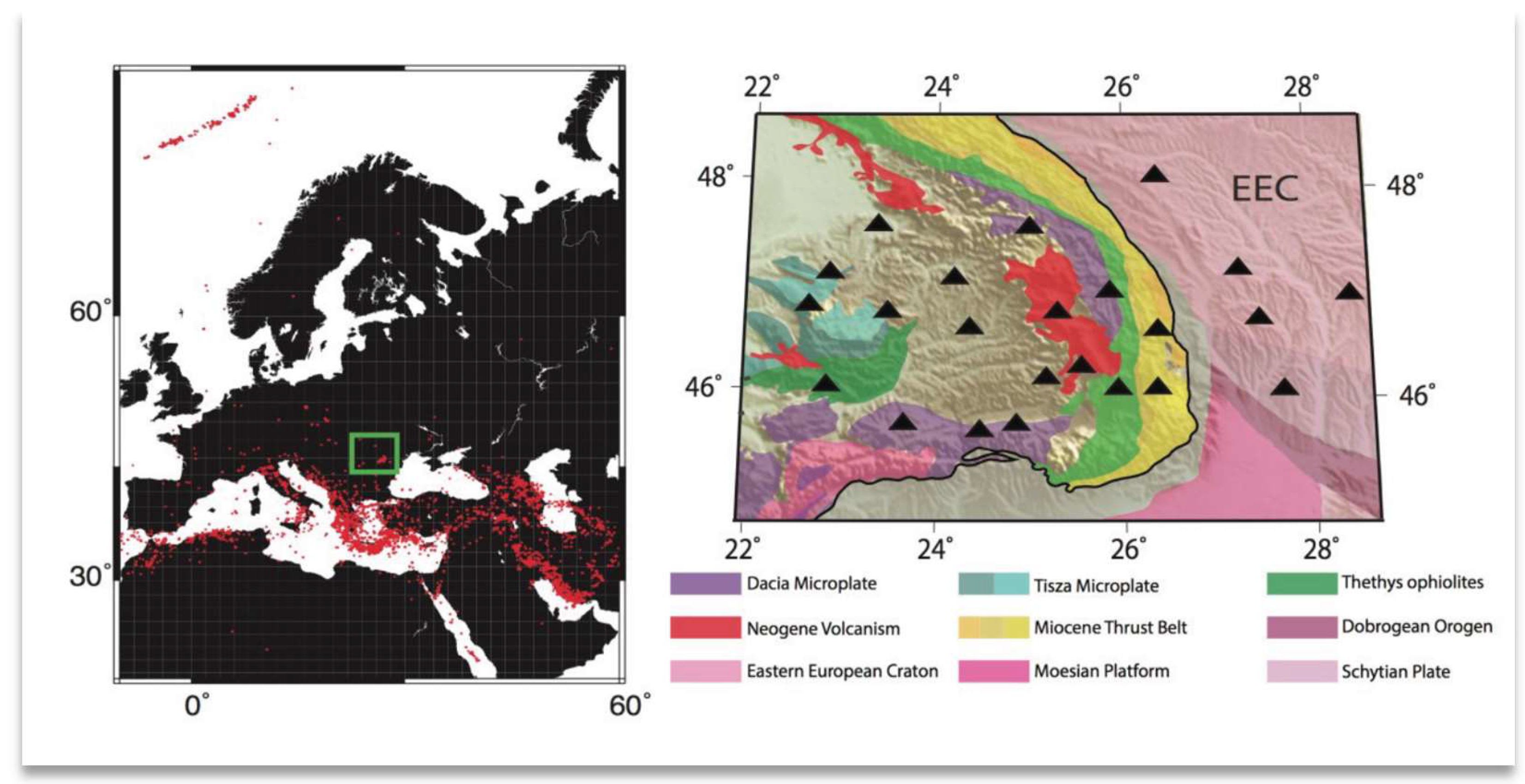
Figure 2.
On the left: Regional map with all seismic sources (red stars) that have produced surface waves with clear dispersion. The path of the waves is color-coded based on their average group velocity recorded at national seismic stations in Romania (blue triangles). On the right: Seismic stations location and the seismic ray paths coverage.
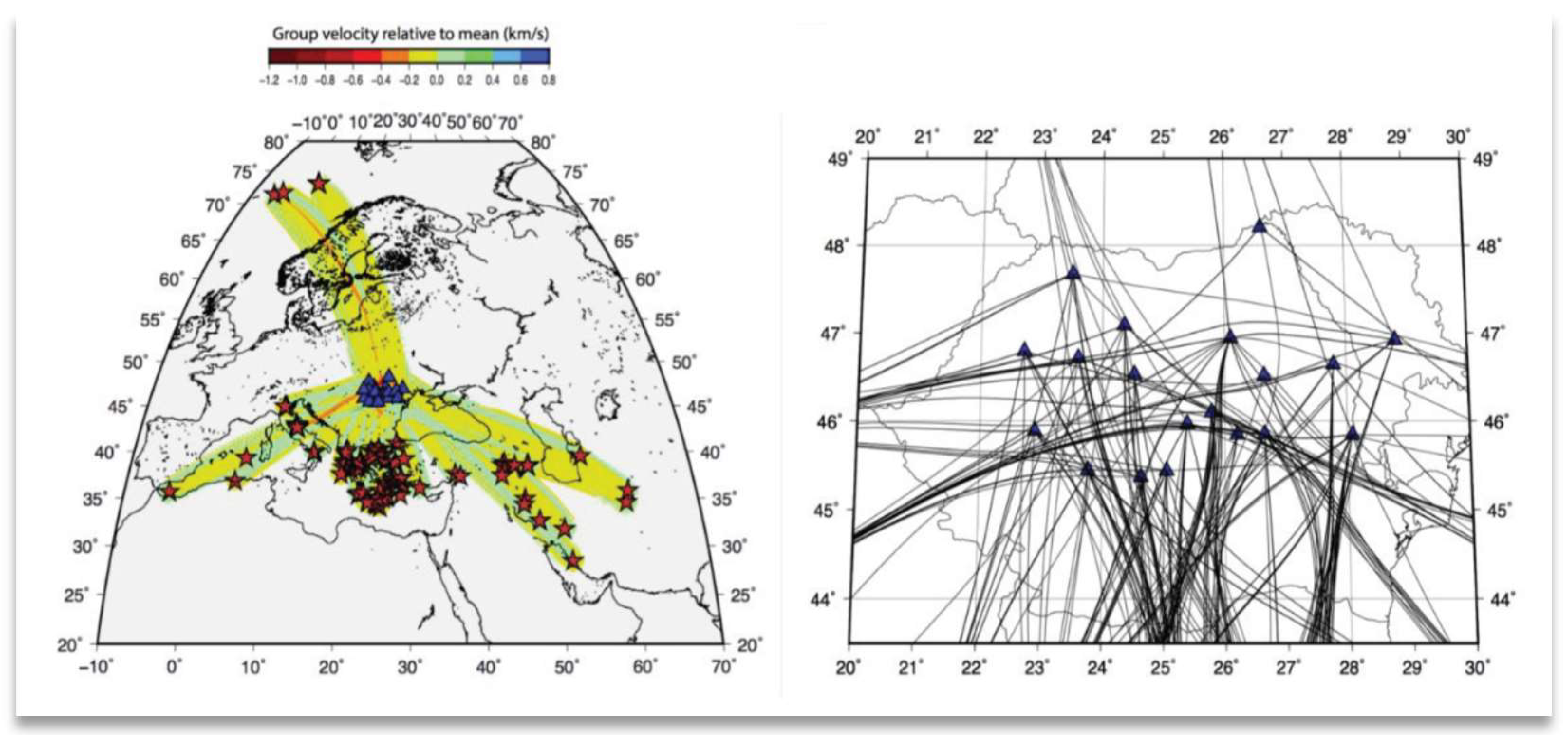
Figure 3.
Left: A graph showing the predicted modal spectral amplitudes in cm-s units(y-axis) versus wave period (x-axis). The squares colored in red are selected by the user and are equivalent to the maximum spectral amplitude; Right: A colored panel showing the energy of surface wave packets as a function of group velocity U in km/s and wave period in s. The white squares represent the peak amplitudes of the signal at discrete periods, manually selected for further analysis. To the right of the modal spectral amplitudes is shown the processed seismogram.
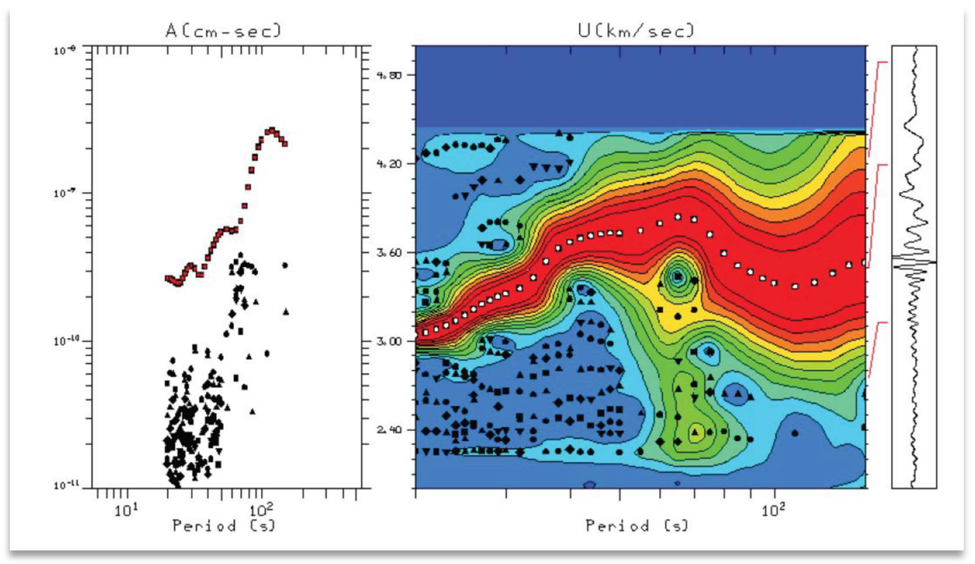
Figure 4.
Left: Rayleigh dispersion curves recorded at the VLDR broadband seismic station, color-coded according to the earthquake azimuth. Right: Rayleigh dispersion curves recorded at the same station, represented polarly based on the earthquake azimuth. The colours represent the group velocity of the waves in km/s, and the circle's radius represents the wave period between 20 and 85s. We note a much smaller interval for which the group velocities of Love waves were extracted compared to Rayleigh waves.
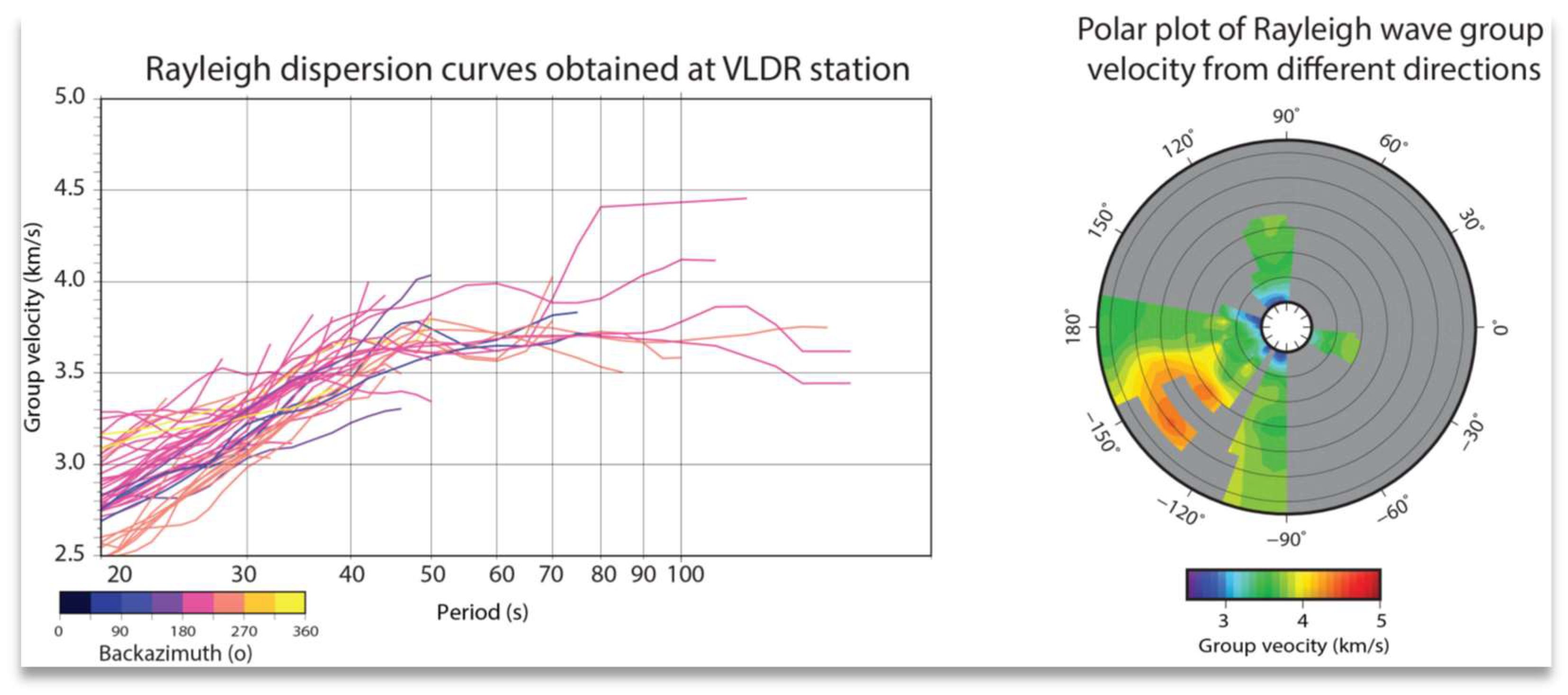
Figure 5.
Histogram showing residual travel times of surface waves after inversion(A). Rayleigh wave group velocity sensitivity kernels.
Figure 5.
Histogram showing residual travel times of surface waves after inversion(A). Rayleigh wave group velocity sensitivity kernels.
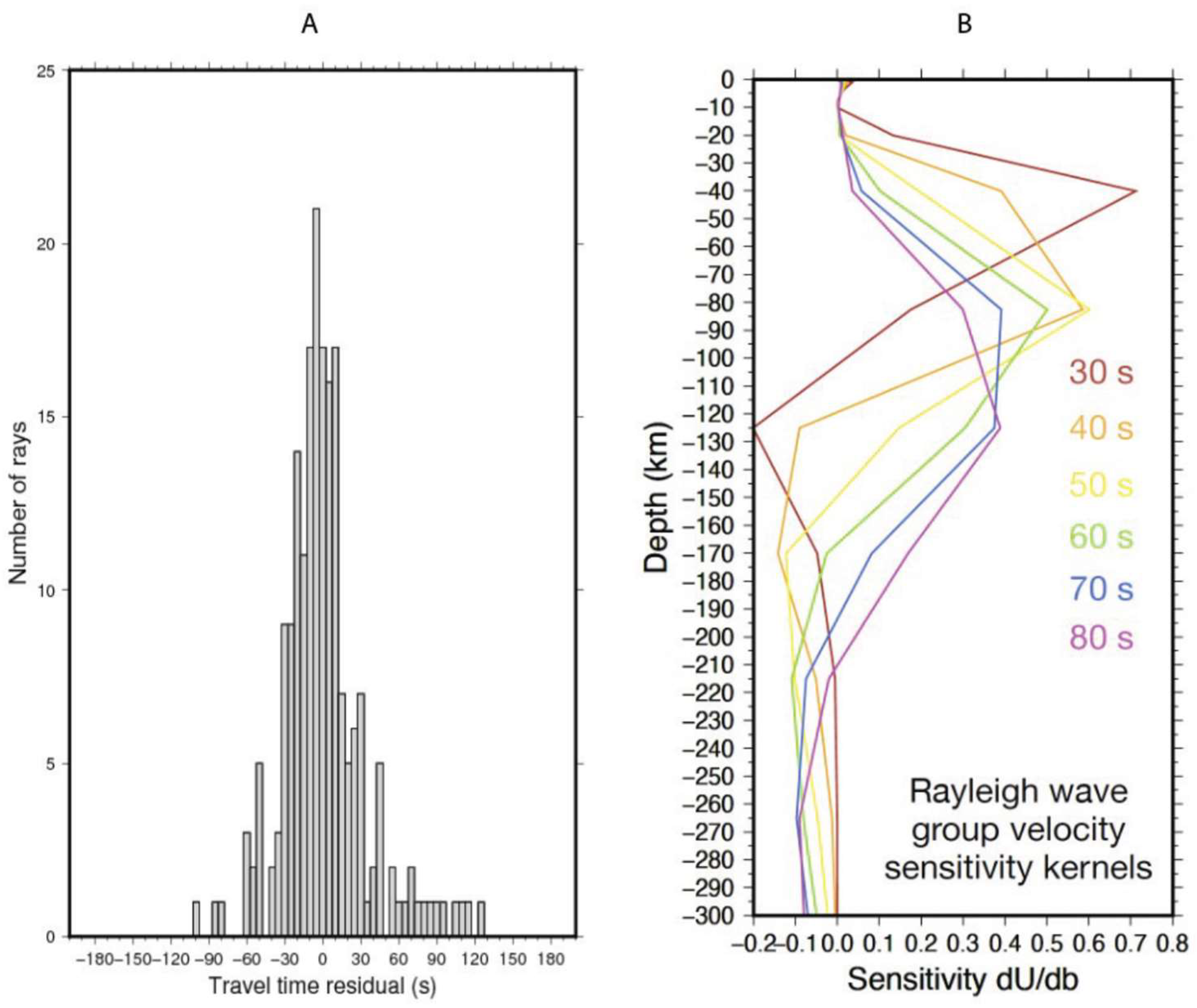
Figure 6.
Rayleigh tomography performed by inverting dispersion curves on the territory of Romania. Each panel represents the lateral variation of group velocity anomalies with respect to the regional average, at selected periods: 30s-80s. The black lines represent the boundaries of major geological units. The points represent intermediate-depth earthquakes from the Vrancea zone at approximate depths where the waves with the selected periods are sensitive.
Disclaimer/Publisher’s Note: The statements, opinions and data contained in all publications are solely those of the individual author(s) and contributor(s) and not of MDPI and/or the editor(s). MDPI and/or the editor(s) disclaim responsibility for any injury to people or property resulting from any ideas, methods, instructions or products referred to in the content. |
© 2025 by the authors. Licensee MDPI, Basel, Switzerland. This article is an open access article distributed under the terms and conditions of the Creative Commons Attribution (CC BY) license (http://creativecommons.org/licenses/by/4.0/).
Copyright: This open access article is published under a Creative Commons CC BY 4.0 license, which permit the free download, distribution, and reuse, provided that the author and preprint are cited in any reuse.


