
Submitted:
10 April 2025
Posted:
11 April 2025
You are already at the latest version
Abstract
Wave energy converters (WECs) have gained significant attention as a promising renewable energy source. Optimal control strategies, crucial for maximizing energy extraction, have traditionally relied on linear models based on small motion assumptions. However, recent studies indicate that these models do not adequately capture the complex dynamics of WECs, especially when large motions are introduced to enhance power absorption. The nonlinear Froude-Krylov (FK) forces, particularly in heaving point absorbers with varying cross-sectional areas, are acknowledged as key contributors to this discrepancy. While high-fidelity computational models are accurate, they are impractical for real-time control applications due to their complexity. This paper presents a parameterized approach for expressing nonlinear FK forces across a wide range of point absorber buoy shapes inspired by implementing real-time, model-based control laws. The model was validated using measured force data for a stationary spherical buoy subjected to regular waves. The FK model was also compared to a closed-form buoyancy model, demonstrating a significant improvement, particularly with high-frequency waves. Incorporating a scattering model further enhanced force prediction, reducing error across the tested conditions. The outcomes of this work contribute to a more comprehensive understanding of FK forces across a broader range of buoy configurations, simplifying the calculation of the excitation force by adopting a parameterized algebraic model and extending this model to accommodate irregular wave conditions.
Keywords:
wave energy converter
; hydrodynamic modeling
; nonlinear hydrodynamics
; excitation force
; froude-krylov force
; point absorber
1. Introduction
The escalating global demand for clean and sustainable energy sources has fueled extensive research to harness the vast potential of ocean waves. With its consistent availability, wave energy is an attractive renewable resource. Site evaluations have confirmed the potential for ocean wave energy resources [1]. Among the various technologies developed, point absorber wave energy converters (PAWEC) have emerged as promising devices capable of efficiently capturing and converting wave energy into electrical power [2]. PAWECs, characterized by buoyant structures tethered to the seabed, offer adaptability to varying wave conditions. The wave-induced vertical motion of its buoyant platform is translated into useful work through a power take-off that can act as either a generator or actuator.
The successful implementation of PAWECs depends on carefully considering design aspects, including buoy size, shape, and mass distribution. Material selection must account for the harsh marine environment, and placement is critical, influenced by factors such as water depth and distance from the shore. Advancements in control systems enable adaptive strategies that maximize energy extraction under varying wave conditions. Improving PAWEC control mechanisms stands out as a crucial avenue with immense potential to improve the feasibility of wave energy utilization [3]. Recent advances highlight the importance of refined control methods, which demonstrate their ability to increase power absorption by up to 20% while simultaneously reducing structural loads [1].
Extensive research on energy-optimal control, particularly for buoy geometries, has been explored. Topics include: establishing upper bounds for energy extraction [4,5,6], impedance matching control [6,7,8,9,10], and exploring both closed-form [11,12] and numerical optimal control solutions [13] such as Model Predictive Control (MPC) [14,15,16,17]. A common theme is the importance of using accurate WEC math models for analysis and control design. Initially, research focused on buoy response regimes that could be approximated using linear differential equations, valid under the assumption of small motion amplitudes. However, a recent shift toward addressing the nonlinear response of buoys [18,19,20] is underway to improve energy extraction, particularly when the objective is to increase power production.
Computational fluid dynamics (CFD) models can accurately capture these nonlinearities, but their application in model-based real-time control laws is impractical [21]. A previous investigation [22] comparing various modeling approaches showed that an important nonlinearity comes from the Froude-Krylov (FK) force, particularly for axisymmetric buoys with varying cross-sectional areas. This insight underscores the importance of understanding and incorporating the nonlinear effects of FK forces in the modeling process to develop effective control strategies.
The FK forces arise from the pressure field around a submerged or partially submerged body as it moves through waves. Specifically, they are associated with the nonlinear effects induced by the varying shape and submersion of the structure. Together with the scattering forces, they constitute the entire non-viscous force exerted on a floating body subjected to regular waves [23]. Developing closed-form, computationally efficient FK force expressions is advantageous for implementing real-time, model-based control strategies. This is especially true for buoys whose shapes result in nonlinear FK forces.
Closed-form nonlinear FK force models have been derived in previous studies [24,25,26], aimed explicitly at using buoy shape effects in model-based control laws for large-motion, nonlinear operating regimes. Giorgi et al. [24] developed a method for generating closed-form FK force expressions using Airy’s wave theory to approximate the pressure on a buoy in regular waves. It has recently been used for model-based control solutions, including sliding model control [27], feedback linearization [28], and latching control [21,29,30].
These studies have taken advantage of various buoy shapes, ranging from conventional spheres and cylinders to more unconventional geometries such as the double cone-shaped buoy [18,28]. The FK force approach by Giorgi et al. has been extended in this paper [24] in several ways, including considering flat bottomed buoys, irregular waves, and a parametrization of a large class of buoy shapes using three parameters. Parameterization allows for rapid evaluation of different geometries, making shape optimization efficient. By generalizing the FK force form, this work provides a powerful tool for improving the design and control of wave energy converters. Furthermore, this paper compares the nonlinear FK model with the buoyancy force approach often used in model-based control [18]. Experiments are used to assess model performance using a spherical buoy subjected to regular waves at several frequencies and amplitudes.
The paper is organized as follows. The model form is introduced in Section 2, including the distinction between the buoyancy and Froude-Krylov terms that are derived in Section 3 and Section 4. Examples of these terms are compared in Section 5, followed by the experimental validation study in Section 6. Some concluding remarks are provided in Section 7.
2. System Description
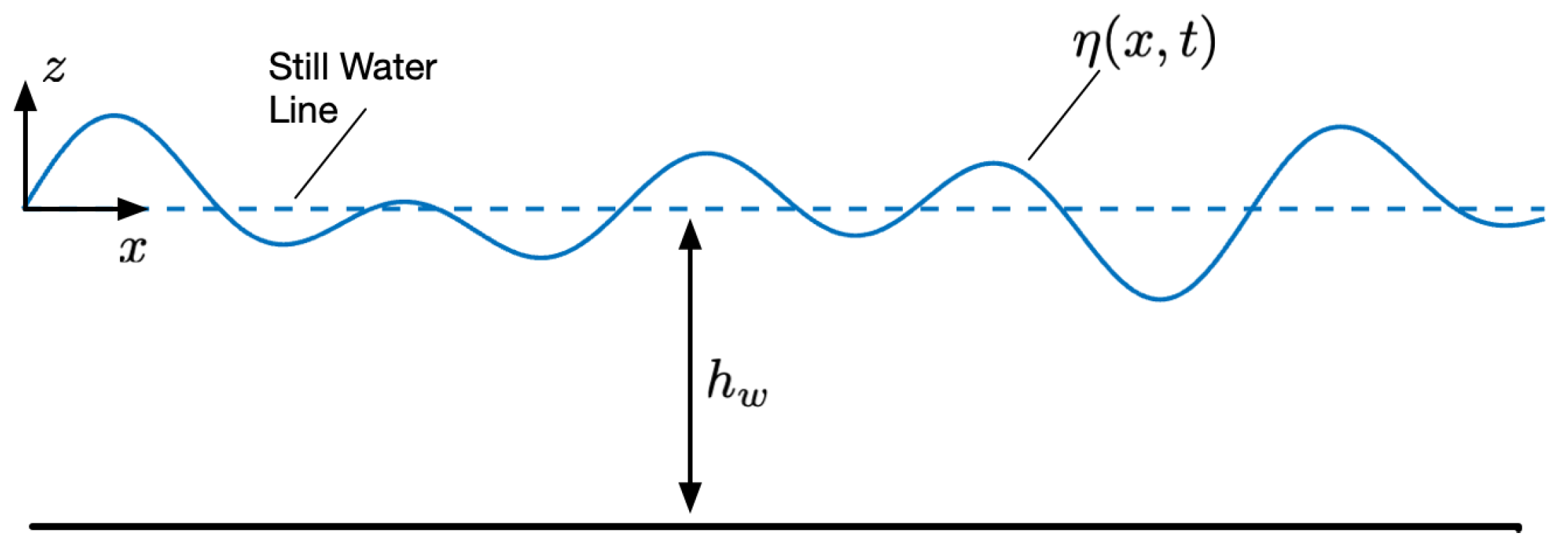
Consider the axisymmetric buoy constrained to heave attached by a PTO to the sea floor in Figure 1. In the configuration shown, the buoy has a positive displacement of its draft line relative to the still-water line. The wave elevation, , is also positive in the figure and is assumed to have the general form of Eq. 1 that allows analysis of both regular and irregular waves.
where ’s ith component has an amplitude, wave number, angular frequency, and phase shift denoted , , , and . The wavelengths, , are assumed to be large compared to the maximum buoy radius, and therefore the free elevation is considered to be locally horizontal, as shown in Figure 1. A body-fixed coordinate system is referenced at the bottom of the buoy. The constant water depth, , is the distance from the sea floor to the still water line and is assumed to be large, though it is shown as small in the figure.
Two model variants will be compared, both having the general form of Eq. 2
where M is the buoy’s mass. Assuming that the buoy does not affect the wave field, the pressure exerted on the buoy by the water is denoted , and the buoy weight is . The scattering force, , when combined with the Froude-Krylov force, is called the diffraction force, ,31] and captures the effect of wave distortion around a fixed buoy [6]. The radiation force, , is due to the energy transfer between the buoy and the water as the buoy moves. Finally, is the power take-off force that adds or removes buoy energy.
The two model variants shown in Eq. 3 are distinguished by how the term of Eq. 2 is treated. In one case, they are replaced by the Froude-Krylov force , and in the other by the buoyancy force .
In both cases, the term will be expressed in a parametric form where a wide range of buoy shapes can be represented using only three independent quantities. In addition, the advantages and disadvantages of the and approaches are discussed. The most significant distinction between them is the assumed motion of the buoy. The derivation assumes small motions, while the approach does not.
3. Derivation of
The derivation of begins by developing the pressure field for irregular waves. The parameterization of the buoy shape is considered next, followed by a representation of in compact form.
3.1. Pressure
The FK term of Eq. 3a, is the integration of the water pressure field, , over the instantaneous wetted surface of the buoy, S, illustrated by the blue shaded region of Figure 2
where is the normal unit vector pointing outwards from the buoy’s surface, is the infinitesimal surface area of the buoy, and the red arrows show the pressure field at a few points. In this snapshot, the buoy’s draft line is below the free elevation, indicating that the buoy is moving relative to the wave.
To derive a closed-form expression for , it is necessary to obtain an expression for that can be integrated. The approach used here is the same as that introduced by Giorgi et al. [24] but with three modifications.
- Consideration of irregular waves of Eq. 1.
- Inclusion of flat-bottomed buoys.
- A three-parameter buoy shape.
The pressure applied to the buoy is derived using linear wave theory in the appendix and given by Eq. 5 where is the water density and g is the gravitational acceleration. Eq. 5 assumes that the fluid is incompressible, inviscid, and irrotational with small particle velocities. Furthermore, it’s valid only for the portion of the buoy below the SWL unrelated to the wave elevation.
The dispersion relationship between the wave number, frequency, and depth, , is also derived in the Appendix and valid under the above mentioned assumptions. If we further assume deep water, it can be approximated as . When applied to Eq. 5, it yields the compact form of Eq. 6.
If the wave is regular with a single amplitude, frequency, and phase shift , Eq. 6 reduces to the equation used by Giorgi et al. in [24].
Finally, it is assumed that the pressure is uniform in x near the buoy, letting us set in Eq. 6. This is important since it allows for closed-form integration to obtain the FK forces and gives the final form of the pressure field of Eq. 8.
where and are the dynamic and static pressure components respectively.
3.2. Pressure Integration and Buoy Shape Parameterization
The approach for generating a closed-form expression for is the same as [24], namely, define the buoy shape by a radius that varies vertically and then integrate the pressure field of Eq. 8 along the radius using cylindrical coordinates. The three additions to the procedure mentioned in Section 3.1 are discussed below. In preparation for a later comparison of FK and buoyancy models, we will write with static and dynamic terms of Eq. 9.
using the "s" and "d" subscripts of Eq. 8.
Figure 3 illustrates the notation used in the derivation where is the revolution profile of the symmetry axis as a function of z that defines the shape of the buoy, is the angle of revolution, is the vertical displacement of the buoy’s draft line relative to the still water line (SWL) at , and h defines the draft line relative to a fixed reference of the buoy, in this case, at the bottom of the buoy.
Unlike previous models [24], Eq. 10 is also supplemented by the pressure acting on the base of the buoy, calculated as the product of the base pressure and its area. The cylindrical coordinate rotation limits and the vertical limits, , are determined by the instantaneous wetted surface below the SWL, or and . The buoy’s non-uniform cross-sectional plane area is . Based on these definitions, and utilizing Eq. 4 with considering only the vertical component of due to heave-only-motion, the forces can be calculated as:
Eq. 10 could be rearranged to obtain the components of the Froude-Krylov (FK) forces as
Substituting Eq. 8 into Eq. 11 and splitting it into static and dynamic components yields Eq. 12.
Closed-form FK force expressions can be created for a wide range of buoy shapes by introducing a special case of a quadric surface given by Eq. 13 where R is the midline buoy radius and is the inverse square of the profile slope’s asymptote in the vertical direction. Equation 13 limits the buoy shapes to being axisymmetric with circular cross sections.
Evaluation of Eq. 12 requires the profile equation obtained from Eq. 13 by shifting the z axis by the buoy displacement and solving for x or y while setting the other variable to zero as shown in Eq. 14.
The area of the circular cross-section is
and is used to describe the pressure effect on buoy shapes with flat bottoms in Eq. 12. Table 1 summarizes the classes of shapes possible with the parameterization of Eq. 14. The value of lets the shape range from an oblate spheroid to the hourglass shape of a hyperboloid. The conical shape is a limiting case with zero radius at the midline. This has little practical application for a buoy but provides insight into the effect of the "necking" of the hyperboloid on nonlinear terms in the final differential equation model. Although h is not part of the parameterization of , it is an important parameter to define the vertical height of the buoy.
Three arrays, , and , whose elements are given in Eq. 16 are introduced to make the closed form expression more compact. Note that contains the components , while is the sum of the components or the free elevation.
Substituting Eq. 14 into and carrying out the integration gives the closed-form expression for of Eq. 17.
Substituting and from Eq. 16 and of Eq. 17 into Eq. 12 provides compact expressions for the static and dynamic FK force, which are combined in Eq. 19.
While this work focuses on closed-form expressions, it is important to note that could be any set of points describing an axisymmetric buoy shape. The integrals of Eq. 12 could be computed numerically in real time as the buoy moves. The form of the FK force would be the same except for a modification of the term.
4. Derivation of
Before developing the model, note that of Eq. 18 is indeed a buoyancy force, but it neglects submersion due to wave elevation. This effect is included in the model below.
The total buoyancy force acting on the buoy is
where is its submerged volume, calculated as the integral of its varying cross-sectional area over the wetted surface.
To account for wave elevation, the area function and the lower integration bound are modified from those of Section 3 to include the instantaneous wave elevation and are shown in Eq. 22
Substituting Eq. 22 into the volume integral of Eq. 21, the buoyancy is given in Eq. 23.
5. Model Form Comparison
The difference between Eq. 23 and of Eq. 19 is how wave elevation, , is used. The expression uses the pressure field containing . However, the boundary conditions of linear wave theory, used to solve Laplace’s equation, are applied to the still water line instead of the free elevation, . This means that the pressure field of Eq. 8 is only valid up to , which is fine as long as both and are small. In contrast, the model can be applied to scenarios where both waves and buoy movement are large, though it omits dynamic pressure effects.
Another way to compare and is to write in two parts where the first term is identical to of Eq. 18
and the second term is an alternate representation of .
To illustrate the differences in the models, Eq. 19 and Eq. 23 are applied to four sample buoy geometries in Table 2 for regular waves, where has one component. The expressions illustrate the effect of the buoy shape on the nature of the nonlinear contribution to the differential equation model of Eq. 3b. For example, the cylinder is linear in , whereas the other shapes have a cubic effect. Compared to the linear term, the relative effect of the nonlinearity depends on R and, to some extent, . The limiting case of the cone-cone shape has no linear term, which means that it has zero stiffness at its equilibrium position with a draft line at its apex. The hourglass shape approximates this behavior for small R.
6. Experimental Validation
The two models of Eq. 3 are evaluated below using regular wave experiments. The objective was to compare with without buoy motion, , and then examine the effect of the scattering force .
6.1. Experimental Setup
The tests were carried out at MTUWave, the wave tank laboratory at Michigan Technological University, shown in Figure 4. A spherical buoy with a 10 cm radius was mounted to a dynamometer with a Sensing Systems load cell to measure the vertical force exerted by incoming waves. The range of the load cell was with a maximum error of and sampled at 100 Hz. The buoy was positioned to have a midline draft and the load cell output was adjusted to zero Newtons.
Two Edinburgh Designs resistance wave gauges, sampled at 128 Hz, were placed on either side of the buoy, laterally aligned with the center of the buoy. The wave gauge measurements were averaged to estimate the wave elevation at the buoy. The wave gauges were calibrated at five vertical positions, so their uncertainty was approximately 0.5 mm.
A dSPACE MicroLabBox was used to log the load cell and provide a synchronization signal to start the wave maker paddles and wave gauge logging. This allowed for the alignment of the data collected across multiple acquisition platforms.
The test conditions are shown in Table 3 and were chosen to exercise the model while not exceeding the capabilities of the wave tank. The nine tests included three different frequencies and amplitudes with wave steepness, the ratio of wave amplitude to wavelength, provided for reference.
6.2. Data Comparison
Wave elevation measurements, , were used to calculate and using Eq. 25, taken from the sphere entry of Table 2, where , , , and .
The calculated and measured forces are compared in Figure 5, Figure 6 and Figure 7. Both models perform well at low frequencies, the uppermost plot in Figure 5 through Figure 7. As the frequency of the wave increases, both models overpredict the force; however, the approach outperforms the model.
The comparison of and with the measured buoy forces ignores the contribution of the scattering force, , of Eq. 3. This force is generally considered negligible when the buoy diameter is significantly smaller than the wavelength [32]. Neglecting aligns well with the 0.2 Hz frequency data, where and the difference between the measured and calculated forces is less than 0.5 N for the 20 mm amplitude case. However, neglecting for the 0.6 Hz and 1.0 Hz cases where is about 40 and 16, respectively, is a possible explanation for the increase in the deviation between the measured and computed forces in the second and third plots in Figure 5 through Figure 7. The maximum deviation for is 1.7 N, and for , it is 0.8 N, both occurring in the 1.0 Hz case of Figure 7.
The total diffraction force, , is defined as the sum of the scattering and Froude-Krylov forces [33].
While the Froude-Krylov component can be obtained as described in Section 3, the scattering force can be extracted from the numerical solution of the diffraction problem, [32]. The complex scattering force coefficients, , were obtained using the boundary element method solver, WAMIT, applied to the spherical buoy using a 972-panel mesh from rad/s in increments of 0.01 rad/s. The real part of is shown in Figure 8 and the time domain force used in the model was created using Eq. 27
for the nine cases of frequencies and amplitudes considered. Eq. 27 is the special case of the irregular wave form, Eq. 28, for a regular wave with a single amplitude, frequency, and phase shift.
Figure 9 compares the effect on the maximum force error of using the expression of Eq. 27 in the model. Each matrix shows the maximum force error between the model and the experiment for three frequencies and three amplitudes. The top two matrices are generated from the data of Figure 5 through Figure 7, and the bottom two matrices show maximum errors between the experiments and the model with . As expected, as the frequency of the wave increases, has a larger effect. It is also readily observed that the model estimates force better than the model as frequency increases. The force is about twice as accurate as the force at 0.6 Hz and four times as accurate at 1.0 Hz.
7. Conclusion and Future Work
Both the and models contain geometry-induced nonlinearity. The model is based on linear wave theory and is applicable to small wave elevations and motion. In contrast, the model, while not as accurate as the model in small-wave conditions, does not assume small waves and motion as long as the waves are far from breaking. Including a scattering force term improves force prediction even for large ratios, e.g., 40.
The ability to express using three parameters that span a variety of buoy shapes is convenient for the design of control laws based on the model and possibly the optimization of the shapes.
Irregular wave model validation needs to be performed to further bound the model applicability. Experiments with different buoy shapes and nonlinear control law implementation are additional areas to explore.
Acknowledgments
Sandia National Laboratories is a multimission laboratory managed and operated by National Technology & Engineering Solutions of Sandia, LLC, a wholly owned subsidiary of Honeywell International Inc., for the U.S. Department of Energy’s National Nuclear Security Administration under contract DE-NA0003525. This paper describes objective technical results and analysis. Any subjective views or opinions that might be expressed in the paper do not necessarily represent the views of the U.S. Department of Energy or the United States Government.
Appendix A
The pressure expression of Eq. 5 is derived below. The approach closely follows that of Chapter 4 of Newman’s Marine Hydrodynamics text [7,33,34] applied to irregular waves.
Consider the situatin of Figure A1 where waves, with free elevation expressed in Eq. A1, propagate along x with no variation in y. The still water line, SWL, corresponds to , and there is a rigid boundary at .
Figure A1.
Illustration of an irregular wave.
Assuming incompressibility the continuity equation is
where u and w are the x and z velocity vector components of a fluid particle located at some Cartesian coordinate point (x,z) and are functions of x, z, and t. If the flow is irrotational, the velocities can be expressed in terms of the velocity potential function,
Combining Eq. A2 and Eq. A3 generates the Laplace Equation in terms of the fluid velocity potential.
If we further assume the fluid is inviscid, then the unsteady form of Bernoulli’s equation can be developed from the continuum equation as
Now we’ll assume the velocities of the fluid particles are small, eliminating the second-order terms of Eq. A5
The that satisfies Eq. A4, with suitable kinematic boundary conditions, can be substituted into Eq. A6 to create the pressure field expression of Eq. 5. At this point, we’ve assumed the flow is incompressible, irrotational, inviscid, with small velocity, but, without any assumption on the wave elevation .
We’ll first consider the kinematic boundary conditions applicable to Eq. A4 based on the z-component of a fluid particle. At the sea floor, the velocity must be zero, giving the boundary condition Eq. A7
and at the free elevation, the fluid particle’s z component of the relative velocity
should be zero. Assuming is small, the free elevation boundary condition is
We will solve the Laplace equation using the separation of variables approach with the assumed form of Eq. A10.
Substituting Eq. A11 into Eq. A4, we find that the must satisfy the differential equations of Eq. A12.
whose solutions are
where the and are constants that can be determined from the boundary conditions.
Consider first the sea floor boundary condition of Eq. A7. The general expression for is
Evaluating Eq. A14 at , the only way Eq. A7 will be satisfied for all time is if the coefficient of the cosine term is zero.
Since the are unique, this becomes n equations where
Substituting Eq. A16 into Eq. A13 gives a new version of
The boundary condition at , Eq. A9, should be used to obtain an expression for the . However, its reliance on the varying makes a closed-form solution elusive at best. Instead, we’ll apply Eq. A9 at the SWL, . Chapter 6 of [33] provides a detailed justification of this approximation using the assumption that is small. This aspect of linear wave theory means that when computing the force of Section 3, the integration of the pressure field should be carried out to the SWL and not the free elevation.
The boundary condition of Eq. A9 requires that
Again, assuming the wave components are independent, we get n equations for the
Substituting Eq. A19 into Eq. A17 gives the the final expression for as
and the velocity potential
Substituting Eq. A21 into Eq. A6 gives the final pressure field
As a final note, we can derive the dispersion equation that relates the frequencies of the wave components to their wave numbers. First, a dynamic boundary condition is created from Bernoulli’s equation by noting that the pressure at should be equal to the atmospheric pressure or
Using the linear wave theory justification of assigning boundaries at the SWL instead of we have
which could be rewritten as
from which we can extract the dispersion equation
that is valid as long as it’s applied to situations where all the assumptions mentioned previously are appropriate.
References
- Aderinto, T.; Li, H. Review on power performance and efficiency of wave energy converters. Energies 2019, 12, 4329.
- Guo, B.; Wang, T.; Jin, S.; Duan, S.; Yang, K.; Zhao, Y. A review of point absorber wave energy converters. Journal of Marine Science and Engineering 2022, 10, 1534.
- Faÿ, F.X.; Henriques, J.C.; Kelly, J.; Mueller, M.; Abusara, M.; Sheng, W.; Marcos, M. Comparative assessment of control strategies for the biradial turbine in the Mutriku OWC plant. Renewable Energy 2020, 146, 2766–2784.
- Budar, K.; Falnes, J. A resonant point absorber of ocean-wave power. Nature 1975, 256, 478–479.
- Falnes, J. A review of wave-energy extraction. Marine structures 2007, 20, 185–201.
- Falnes, J.; Kurniawan, A. Ocean waves and oscillating systems: linear interactions including wave-energy extraction; Vol. 8, Cambridge university press, 2020.
- Korde, U.A.; Ringwood, J. Hydrodynamic control of wave energy devices; Cambridge University Press, 2016.
- Faedo, N.; Pasta, E.; Carapellese, F.; Orlando, V.; Pizzirusso, D.; Basile, D.; Sirigu, S.A. Energy-maximising experimental control synthesis via impedance-matching for a multi degree-of-freedom wave energy converter. IFAC-PapersOnLine 2022, 55, 345–350.
- Lattanzio, S.; Scruggs, J. Maximum power generation of a wave energy converter in a stochastic environment. In Proceedings of the 2011 IEEE international conference on control applications (CCA). IEEE, 2011, pp. 1125–1130.
- Bacelli, G.; Nevarez, V.; Coe, R.G.; Wilson, D.G. Feedback resonating control for a wave energy converter. IEEE Transactions on Industry Applications 2019, 56, 1862–1868.
- Yassin, H.; Demonte Gonzalez, T.; Nelson, K.; Parker, G.; Weaver, W. Optimal Control of Nonlinear, Nonautonomous, Energy Harvesting Systems Applied to Point Absorber Wave Energy Converters. Journal of Marine Science and Engineering 2024, 12, 2078.
- Zou, S.; Abdelkhalik, O.; Robinett, R.; Bacelli, G.; Wilson, D. Optimal control of wave energy converters. Renewable energy 2017, 103, 217–225.
- Abdelkhalik, O.; Darani, S. Optimization of nonlinear wave energy converters. Ocean Engineering 2018, 162, 187–195.
- Li, G.; Belmont, M.R. Model predictive control of sea wave energy converters–Part I: A convex approach for the case of a single device. Renewable Energy 2014, 69, 453–463.
- Brekken, T.K. On model predictive control for a point absorber wave energy converter. In Proceedings of the 2011 IEEE Trondheim PowerTech. IEEE, 2011, pp. 1–8.
- Zou, S.; Abdelkhalik, O.; Robinett, R.; Korde, U.; Bacelli, G.; Wilson, D.; Coe, R. Model Predictive Control of parametric excited pitch-surge modes in wave energy converters. International journal of marine energy 2017, 19, 32–46.
- Demonte Gonzalez, T.; Anderlini, E.; Yassin, H.; Parker, G. Nonlinear Model Predictive Control of Heaving Wave Energy Converter with Nonlinear Froude–Krylov Forces. Energies 2024, 17, 5112.
- Wilson, D.G.; Robinett III, R.D.; Bacelli, G.; Abdelkhalik, O.; Coe, R.G. Extending complex conjugate control to nonlinear wave energy converters. Journal of Marine Science and Engineering 2020, 8, 84.
- Richter, M.; Magana, M.E.; Sawodny, O.; Brekken, T.K. Nonlinear model predictive control of a point absorber wave energy converter. IEEE Transactions on Sustainable Energy 2012, 4, 118–126.
- Darani, S.; Abdelkhalik, O.; Robinett, R.D.; Wilson, D. A hamiltonian surface-shaping approach for control system analysis and the design of nonlinear wave energy converters. Journal of Marine Science and Engineering 2019, 7, 48.
- Giorgi, G.; Ringwood, J.V. Implementation of latching control in a numerical wave tank with regular waves. Journal of Ocean Engineering and Marine Energy 2016, 2, 211–226.
- Giorgi, G.; Ringwood, J.V. Nonlinear Froude-Krylov and viscous drag representations for wave energy converters in the computation/fidelity continuum. Ocean Engineering 2017, 141, 164–175.
- Faltinsen, O. Sea loads on ships and offshore structures; Vol. 1, Cambridge university press, 1993.
- Giorgi, G.; Ringwood, J.V. Computationally efficient nonlinear Froude–Krylov force calculations for heaving axisymmetric wave energy point absorbers. Journal of Ocean Engineering and Marine Energy 2017, 3, 21–33.
- Giorgi, G.; Ringwood, J.V. A Compact 6-DoF Nonlinear Wave Energy Device Model for Power Assessment and Control Investigations. IEEE Transactions on Sustainable Energy 2019, 10, 119–126. [CrossRef]
- Giorgi, G.; Sirigu, S.; Bonfanti, M.; Bracco, G.; Mattiazzo, G. Fast nonlinear Froude–Krylov force calculation for prismatic floating platforms: a wave energy conversion application case. Journal of Ocean Engineering and Marine Energy 2021, 7, 439–457.
- Demonte Gonzalez, T.; Parker, G.G.; Anderlini, E.; Weaver, W.W. Sliding mode control of a nonlinear wave energy converter model. Journal of Marine Science and Engineering 2021, 9, 951.
- Yassin, H.; Demonte Gonzalez, T.; Parker, G.; Wilson, D. Effect of the Dynamic Froude–Krylov Force on Energy Extraction from a Point Absorber Wave Energy Converter with an Hourglass-Shaped Buoy. Applied Sciences 2023, 13, 4316.
- Penalba, M.; Giorgi, G.; Ringwood, J.V. Mathematical modelling of wave energy converters: A review of nonlinear approaches. Renewable and Sustainable Energy Reviews 2017, 78, 1188–1207. [CrossRef]
- Giorgi, G.; Ringwood, J.V. Comparing nonlinear hydrodynamic forces in heaving point absorbers and oscillating wave surge converters. Journal of Ocean Engineering and Marine Energy 2018, 4, 25–35.
- WAMIT, Inc. The State of the Art in Wave Interaction Analysis, 2023.
- Korde, U.A.; Ringwood, J. Hydrodynamic Control of Wave Energy Devices; Cambridge University Press: Cambridge, 2016. [CrossRef]
- Newman, J.N. Marine Hydrodynamics; The MIT Press, 1977. [CrossRef]
- Dingemans, M.W. Water wave propagation over uneven bottoms: Linear wave propagation; Vol. 13, World Scientific, 2000.
Figure 1.
Illustration of an axisymmetric buoy and the notation used for its model.
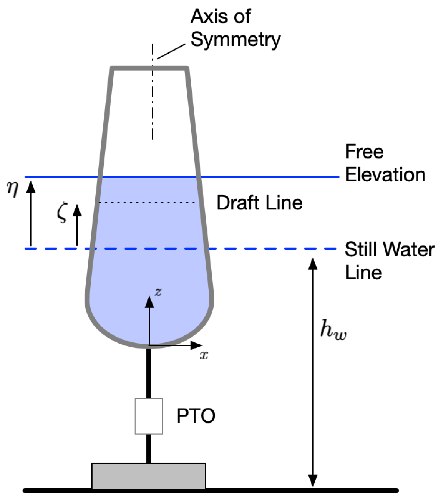
Figure 2.
Illustration of the pressure field acting on the buoy over its wetted surface.
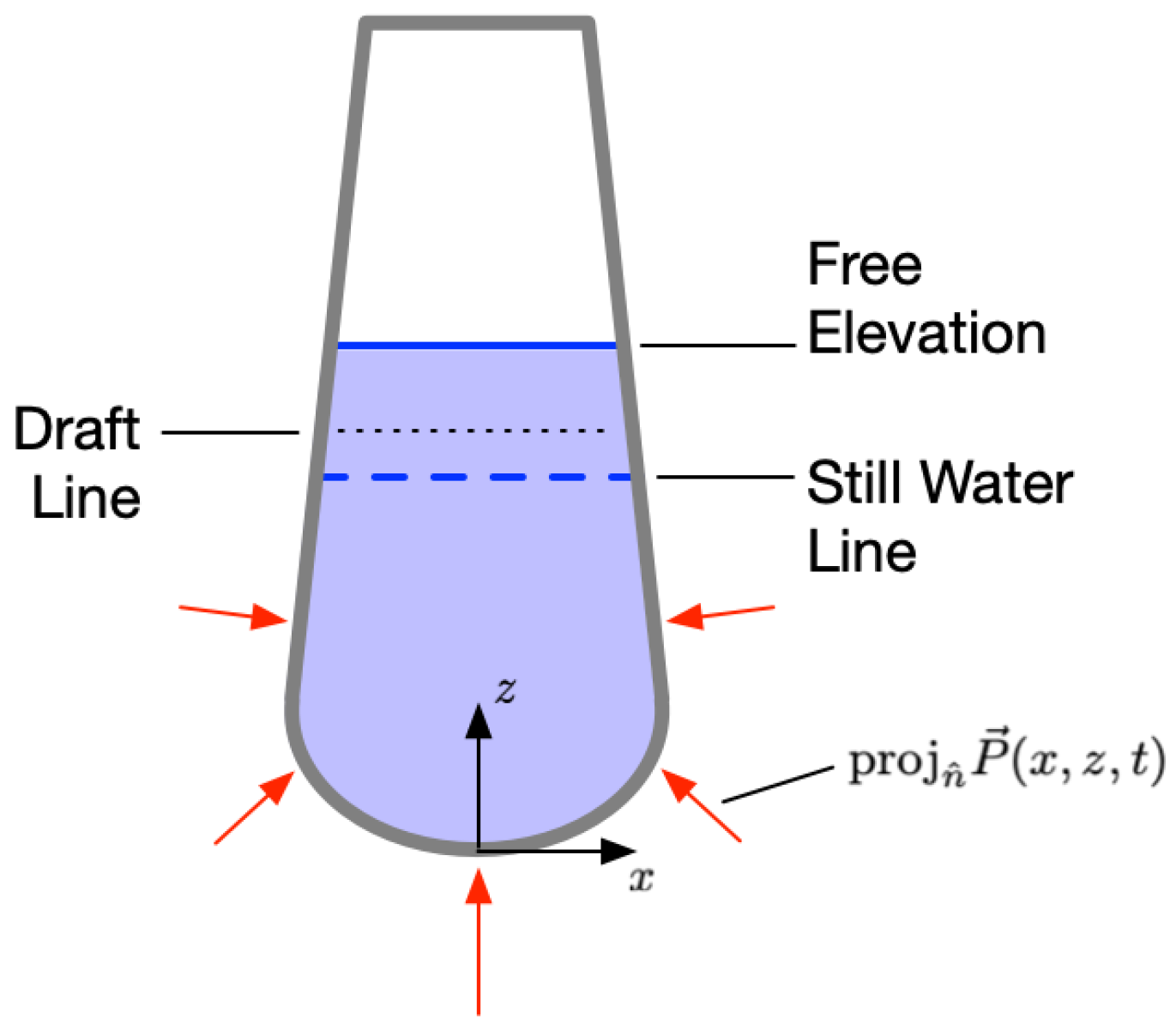
Figure 3.
2D display of the parameters used to derive the forces.
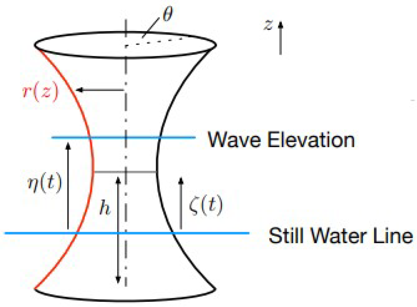
Figure 4.
Experimental setup at the Michigan Tech wave tank (MTUWave) with Wave Gauge (WG) positions.
Figure 4.
Experimental setup at the Michigan Tech wave tank (MTUWave) with Wave Gauge (WG) positions.
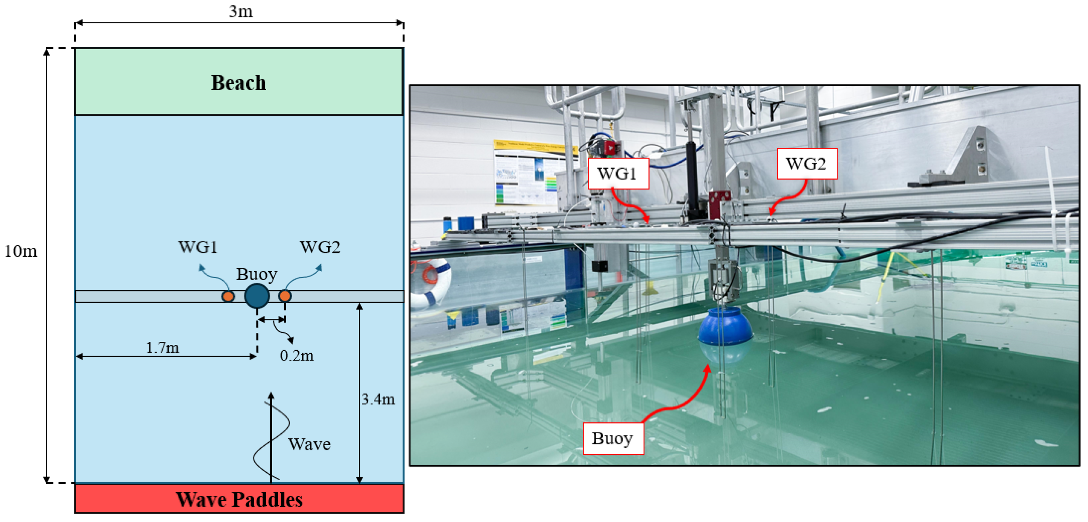
Figure 5.
Comparison of measured and modeled buoy forces for mm at frequencies of 0.2, 0.6, and 1.0 Hz.
Figure 5.
Comparison of measured and modeled buoy forces for mm at frequencies of 0.2, 0.6, and 1.0 Hz.
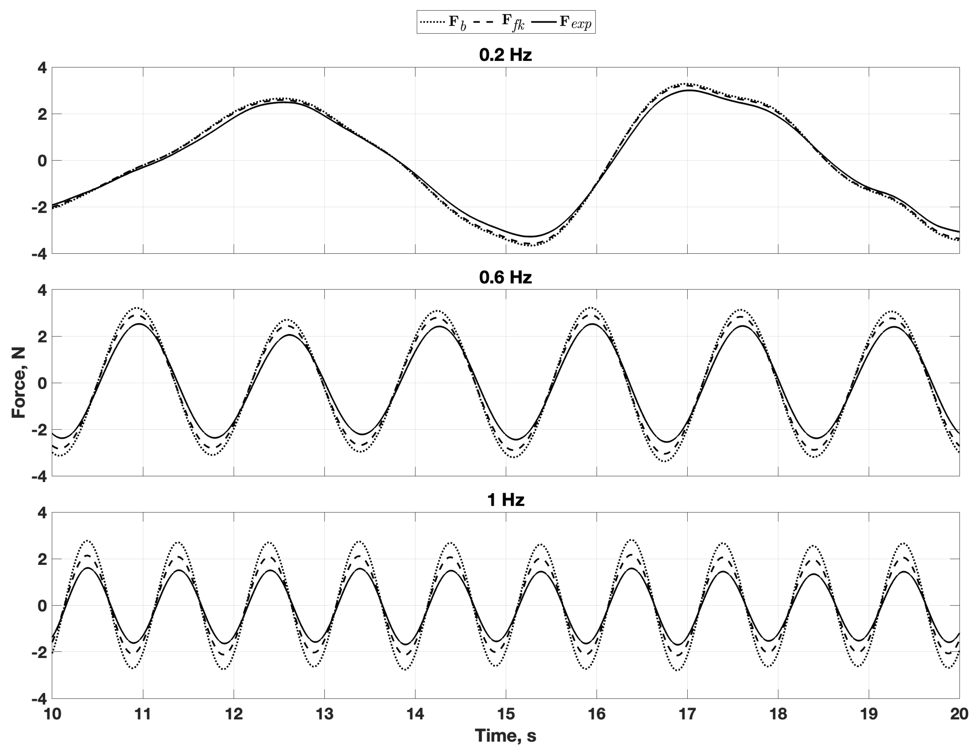
Figure 6.
Comparison of measured and modeled buoy forces for mm at frequencies of 0.2, 0.6, and 1.0 Hz.
Figure 6.
Comparison of measured and modeled buoy forces for mm at frequencies of 0.2, 0.6, and 1.0 Hz.
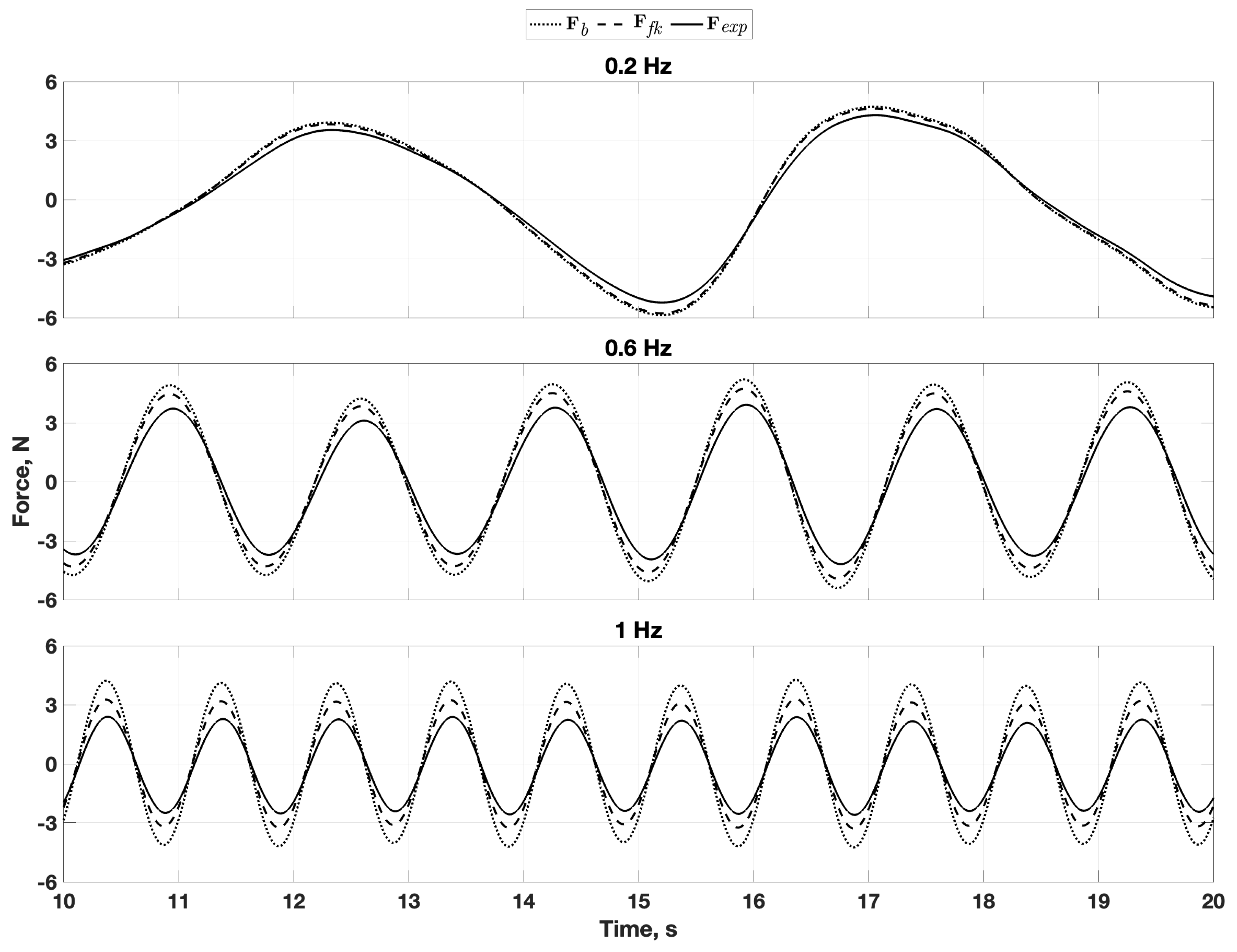
Figure 7.
Comparison of measured and modeled buoy forces for mm at frequencies of 0.2, 0.6, and 1.0 Hz.
Figure 7.
Comparison of measured and modeled buoy forces for mm at frequencies of 0.2, 0.6, and 1.0 Hz.
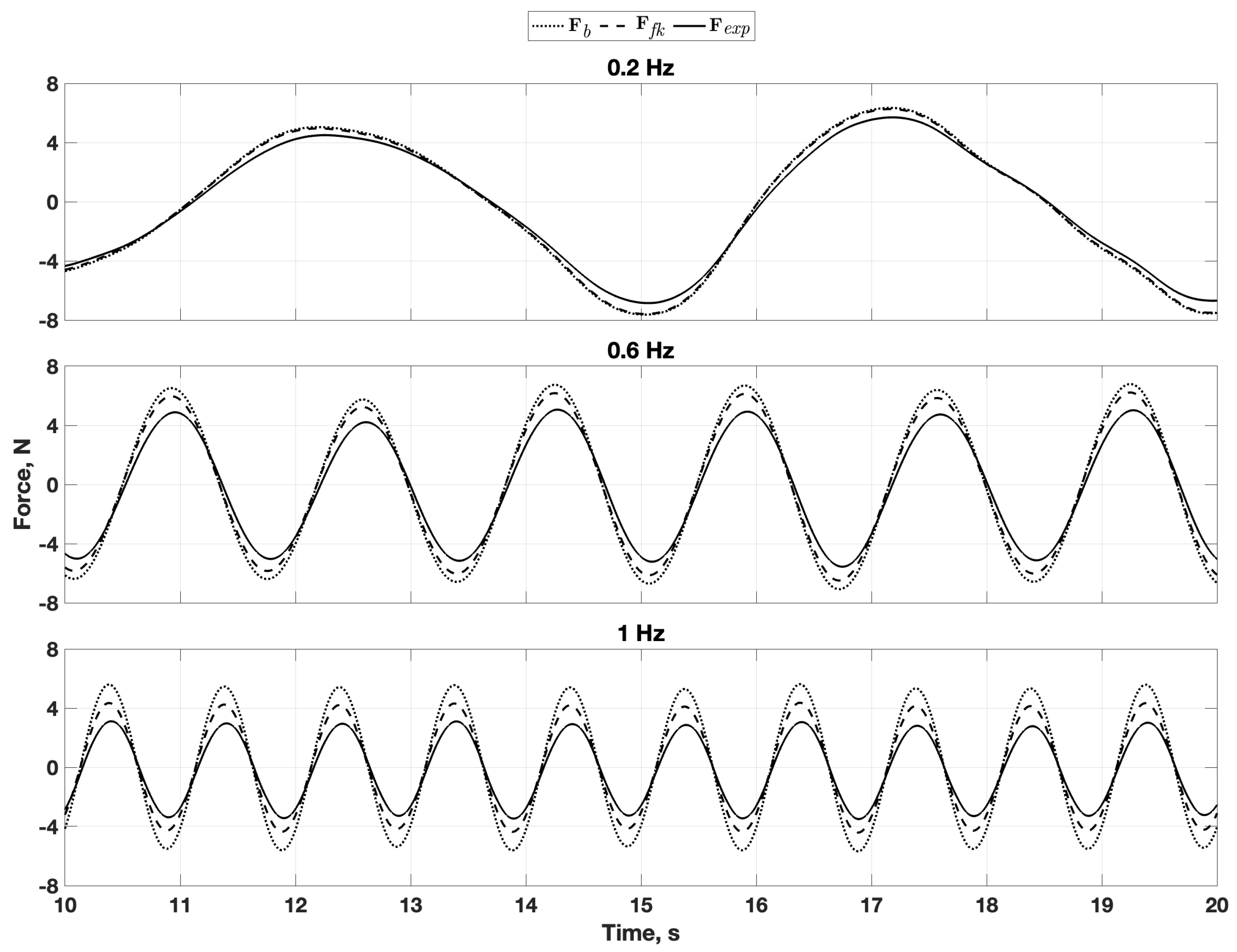
Figure 8.
Real scattering coefficient of a 0.1 m spherical buoy. The experiment frequencies of 0.2, 0.6, and 1.0 Hz correspond to 1.3, 3.8, and 6.3 rad/s and are shown with corresponding coefficients of -2.98, -24.23 and -48.82 respectively.
Figure 8.
Real scattering coefficient of a 0.1 m spherical buoy. The experiment frequencies of 0.2, 0.6, and 1.0 Hz correspond to 1.3, 3.8, and 6.3 rad/s and are shown with corresponding coefficients of -2.98, -24.23 and -48.82 respectively.
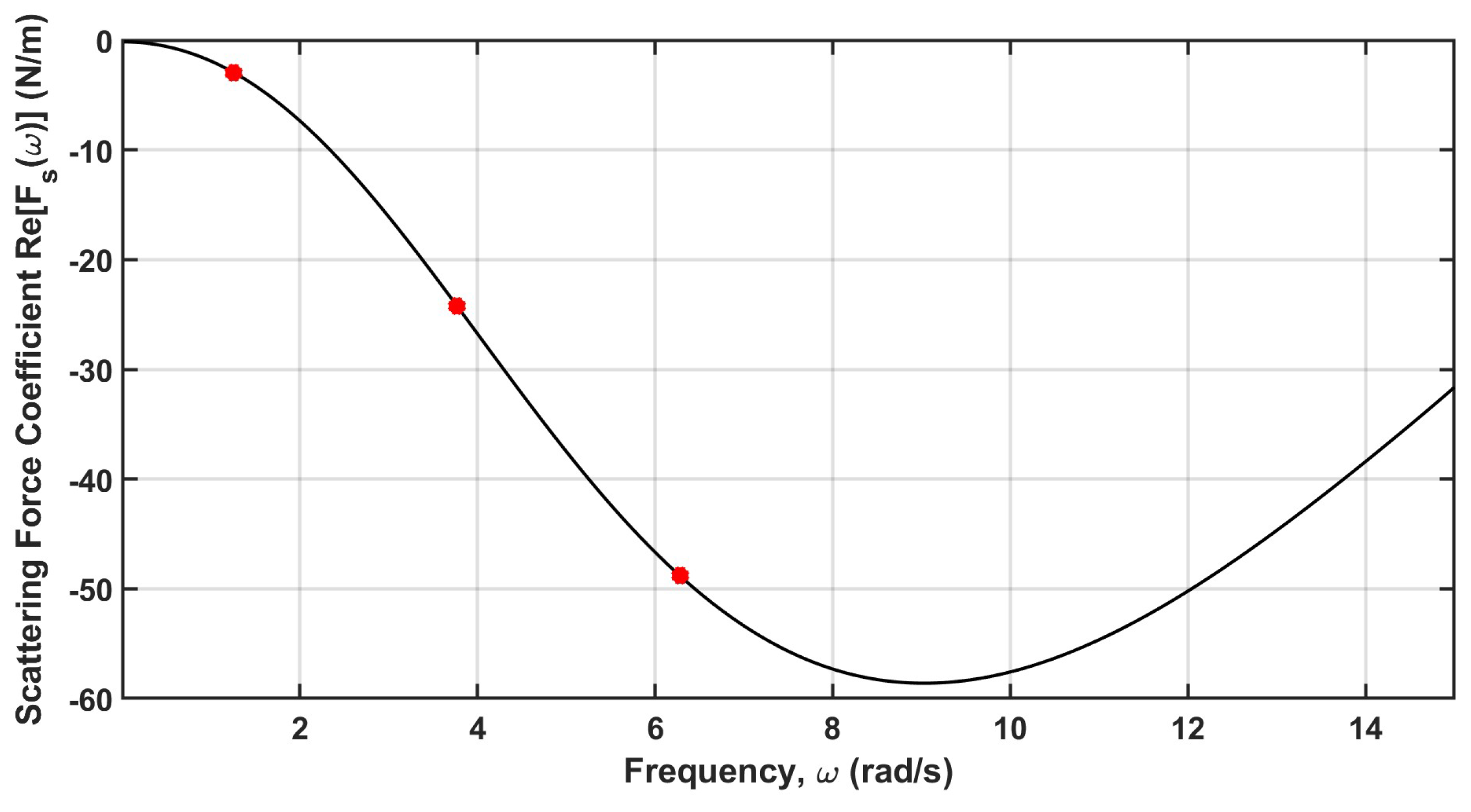
Figure 9.
Comparison of the nine experiments with four different models: (upper left), (upper right), (lower left) and (lower right). The values in each square are the maximum force difference between the experiment and the model.
Figure 9.
Comparison of the nine experiments with four different models: (upper left), (upper right), (lower left) and (lower right). The values in each square are the maximum force difference between the experiment and the model.
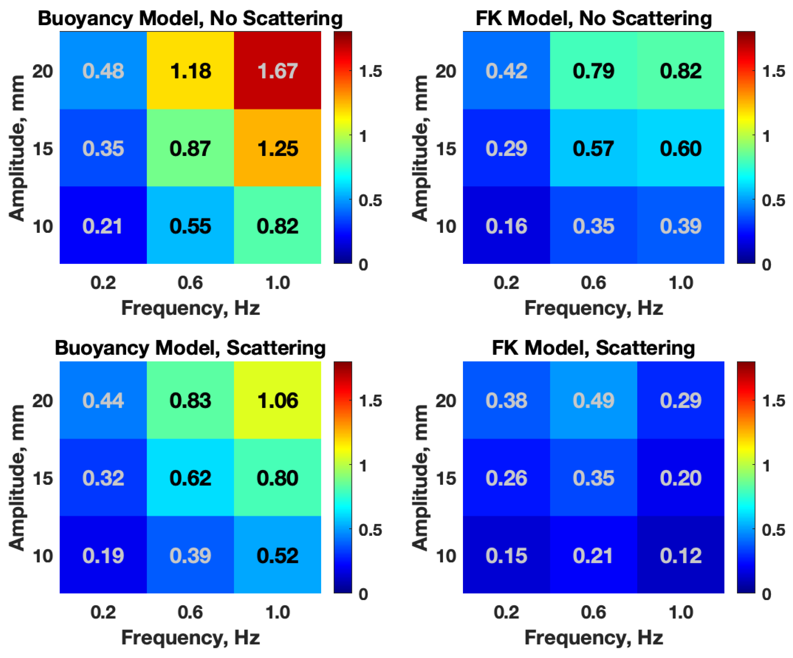
Figure 10.
Comparison of measured and modeled buoy forces for mm at frequencies of 0.2, 0.6, and 1.0 Hz where was included in the model.
Figure 10.
Comparison of measured and modeled buoy forces for mm at frequencies of 0.2, 0.6, and 1.0 Hz where was included in the model.
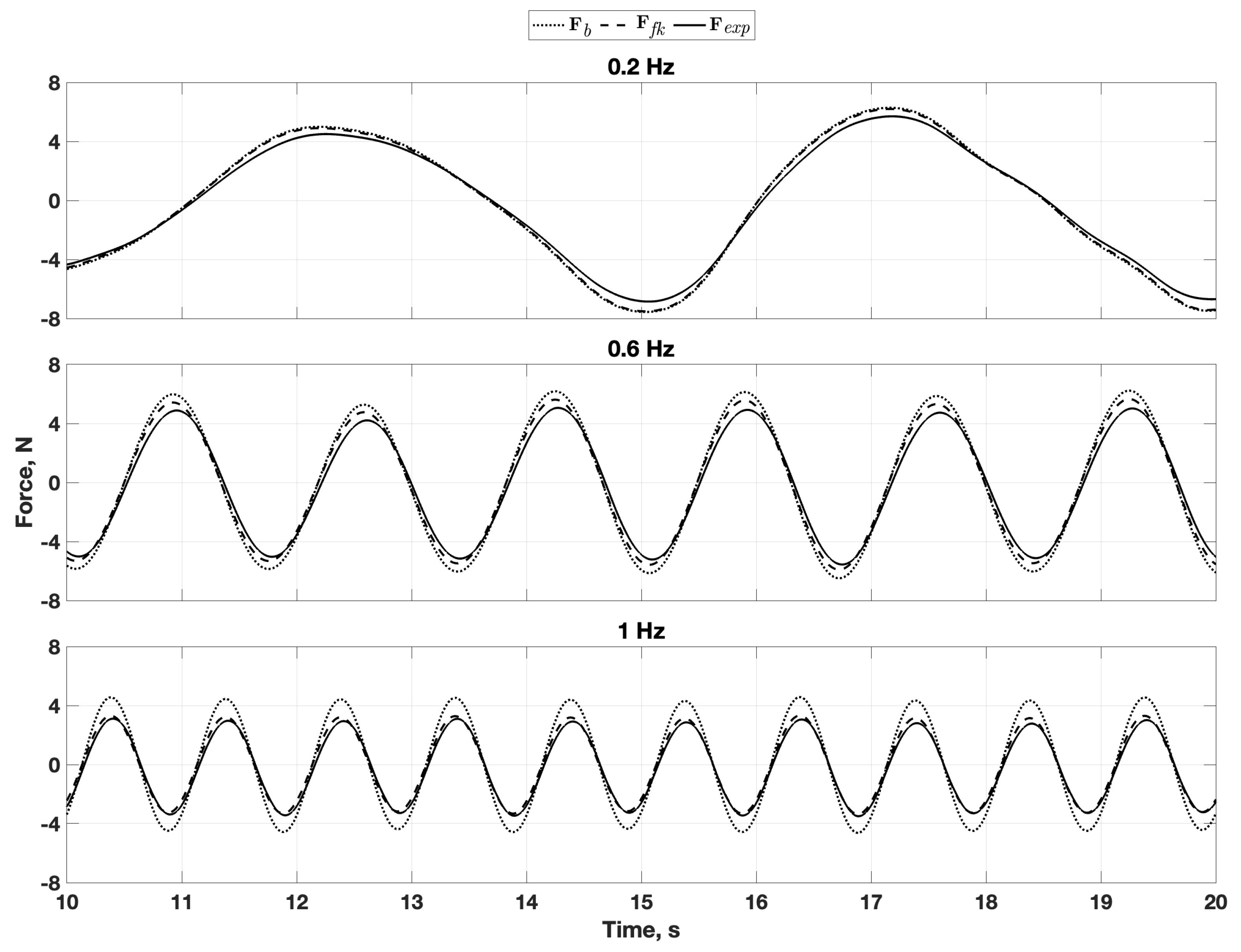

Table 1.
Buoy Shapes and Corresponding Parameters.
| Shape | R | h | |
| Spheroid, Oblate | Free | ||
| Sphere | Free | R | |
| Spheroid, Prolate | Free | ||
| Cylinder | 0 | Free | Free |
| Hyperboloid (Hourglass) | Free | Free | |
| Cone-Cone | 0 | Free |
Table 2.
buoyancy model and Froude-Krylov Forces for Different Buoy Shapes in Regular Waves.
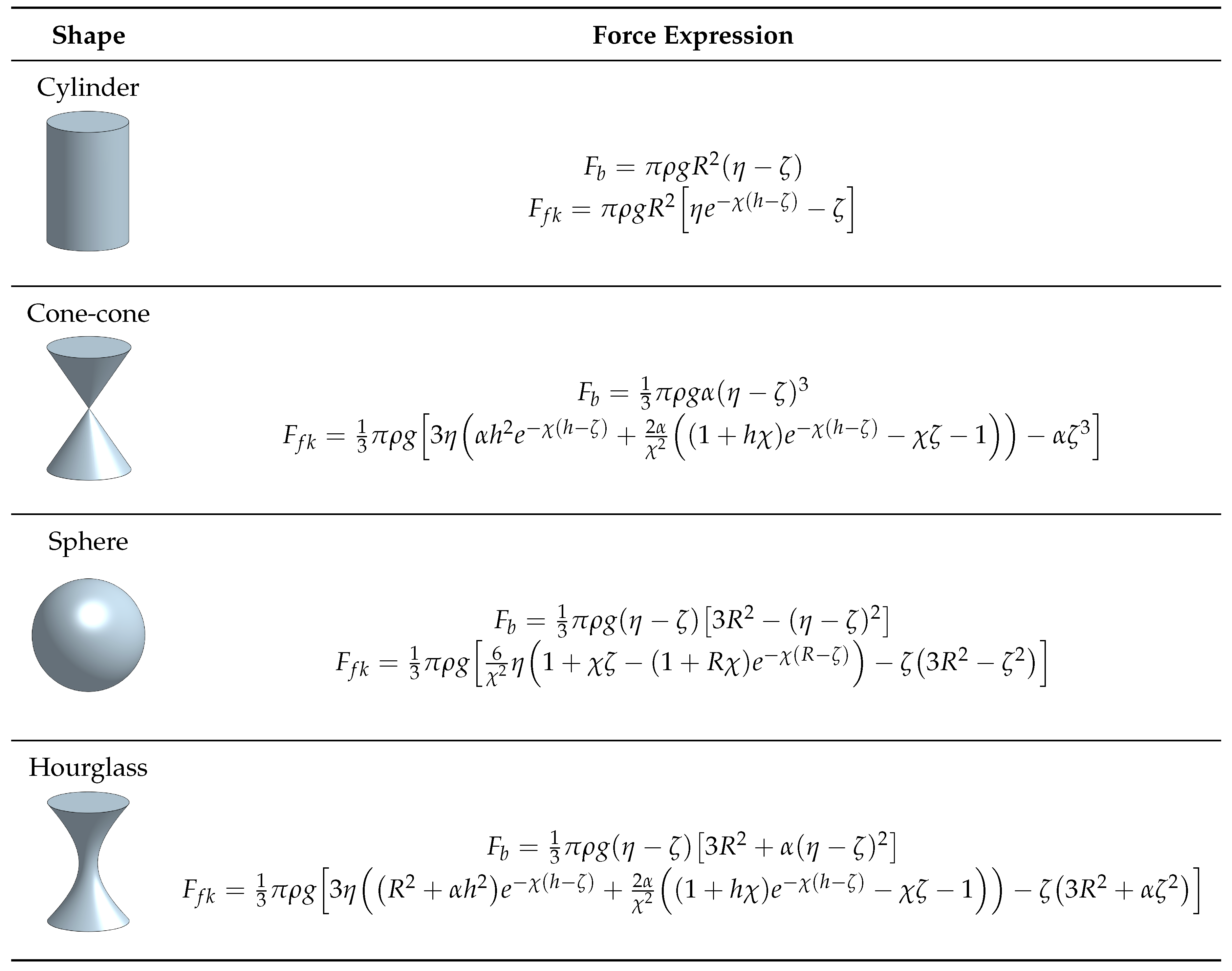 |
Table 3.
Regular wave characteristics used for model comparison experiments. The first two columns are the independent parameters, while the remaining columns are for reference.
Table 3.
Regular wave characteristics used for model comparison experiments. The first two columns are the independent parameters, while the remaining columns are for reference.
| Frequency f, Hz | Amplitude A, mm | Number , 1/m | Length , m | Steepness |
| 0.2 | [10, 15, 20] | 0.4 | 15.2 | [0.0005, 0.0008, 0.001] |
| 0.6 | [10, 15, 20] | 1.6 | 4.0 | [0.005, 0.007, 0.009] |
| 1.0 | [10, 15, 20] | 4.0 | 1.6 | [0.013, 0.019, 0.026] |
Disclaimer/Publisher’s Note: The statements, opinions and data contained in all publications are solely those of the individual author(s) and contributor(s) and not of MDPI and/or the editor(s). MDPI and/or the editor(s) disclaim responsibility for any injury to people or property resulting from any ideas, methods, instructions or products referred to in the content. |
© 2025 by the authors. Licensee MDPI, Basel, Switzerland. This article is an open access article distributed under the terms and conditions of the Creative Commons Attribution (CC BY) license (http://creativecommons.org/licenses/by/4.0/).
Copyright: This open access article is published under a Creative Commons CC BY 4.0 license, which permit the free download, distribution, and reuse, provided that the author and preprint are cited in any reuse.


