
Submitted:
07 April 2025
Posted:
08 April 2025
You are already at the latest version
Abstract
With the increasing number of illegal radio stations, connected cars, and IoT devices, high-accuracy radio source localization techniques are in demand. Traditional methods such as GPS positioning and triangulation suffer from accuracy degradation in NLOS (non-line-of-sight) environments due to obstructions. In contrast, the fingerprinting method builds a database of pre-collected radio information and estimates the source location via pattern matching, maintaining relatively high accuracy in NLOS environments. This study aims to improve the accuracy of fingerprinting-based localization by optimizing UAV flight paths. Previous research mainly relied on RSSI-based localization, but we introduce an AOA model considering AOA (Angle of Arrival) and EOA (Elevation of Arrival), as well as a HYBRID model that integrates multiple radio features with weighting. Using Wireless Insite, we conducted ray-tracing simulations based on the Institute of Science Tokyo’s Ookayama campus and optimized UAV flight paths with PSO (Particle Swarm Optimization). Results show that the HYBRID model achieved the highest accuracy, limiting the maximum error to 20m. Sequential estimation improved accuracy for high-error sources, particularly when RSSI was used first, followed by AOA or HYBRID. Future work includes estimating unknown frequency sources, refining sequential estimation, and implementing cooperative localization.
Keywords:
Radio source localization
; fingerprinting
; RSSI
; AOA
; EOA
1. Background
In recent years, the widespread adoption of 4G (Fourth-Generation Mobile Communication System) and the full-scale introduction of 5G (Fifth-Generation Mobile Communication System) have led to a rapid increase in the use of mobile devices and IoT (Internet of Things) devices. As a result, various wireless communication technologies, such as next-generation mobility solutions like autonomous vehicles and connected cars, smart homes, and industrial IoT, have become essential infrastructure in daily life. To meet these societal demands, radio wave usage has expanded rapidly [1]. However, alongside the growing adoption of radio wave usage, the inappropriate use of frequency bands and illegal radio stations that violate Japan’s Radio Act have also increased, as shown in Figure 1. This has raised concerns about serious communication disruptions caused by unauthorized radio stations [2]. Figure 1 indicates that while the number of illegal radio stations has been decreasing over the past two years (2022 and 2023), only about one-fourth of them have been successfully detected and addressed. Therefore, the development of a high-precision and highly efficient radio source localization system is required [2].
The DEURAS (Detecting Unlicensed Radio Stations) system, shown in Figure 2, is the current illegal radio station localization system operated by the Ministry of Internal Affairs and Communications. The DEURAS system estimates the approximate location of transmission sources using received radio wave information collected from fixed sensors installed on rooftops of buildings. Following this initial estimation, vehicles are then deployed for on-site investigation. To reduce search costs, a high-precision localization system capable of identifying transmission sources within a short time is required, considering that radio stations may move over time.
1.1. Objective
This paper aims to estimate the coordinates of a radio wave source using pattern matching of position fingerprints with a database created by ray tracing simulation. UAVs fly along an optimal path to minimize estimation errors between actual and estimated positions. The position fingerprinting method constructs a database with pre-measured RSSI, AOA, and EOA data. This method improves position estimation accuracy even in NLoS environments. The study proposes using UAVs as sensors to increase the dimensions of the position fingerprint database cost-effectively and improve estimation accuracy by obtaining LoS signals. The UAV’s flight path is optimized as a problem to achieve high efficiency and accuracy. This research builds on previous works by Tanaka and Kamei, integrating RSSI, AOA, and a hybrid method into the estimation model.
1.2. Related Work and the Position of This Research
This section discusses the positioning of this research in relation to previous and related studies. Tanaka’s study [4] and Kamei’s study [5] serve as precursors to this research. Tanaka performed position estimation using a radio wave fingerprinting method employing RSSI and AOA with UAV sensors at Okayama Campus of Tokyo Institute of Technology. Kamei built upon Tanaka’s model by optimizing the UAV’s trajectory path using RSSI, which significantly improved estimation accuracy. Additionally, related studies include [6,7,8,9]. In this research, a hybrid method integrating not only RSSI but also AOA with weighted integration was added to Tanaka’s and Kamei’s models. Further, adjustments to the circular trajectory radii drawn by the UAV and sequential estimation were employed to assess and evaluate their impact on estimation accuracy via radio information.
2. Materials and Methods
2.1. Overall Flowchart
The flow of the proposed method is as follows.
Figure 3.
Flowchart of the proposed method.
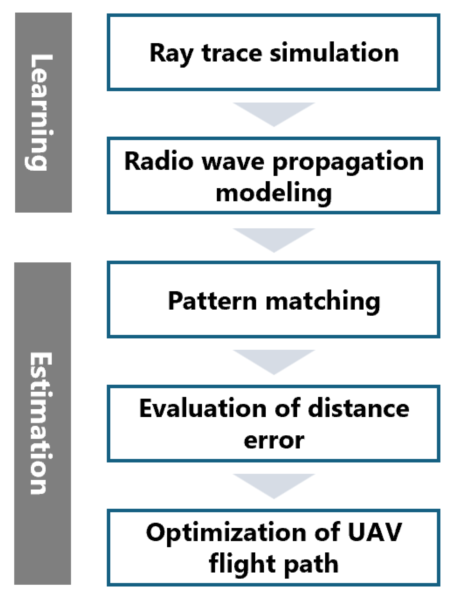
Initially, in the learning phase of the location fingerprinting method, a radio wave propagation simulation is conducted in an urban environment. Since the radio wave propagation simulation only provides sparse data due to its computational cost constraints, regression-based radio wave propagation modeling is employed to supplement continuous data. This approach enables the utilization of optimization techniques for continuous functions, such as particle swarm optimization and genetic algorithms, in subsequent steps.
Next, in the estimation phase, pattern matching between the location fingerprint database and the received signal from the target is performed. Based on the matching results, the positioning error is calculated and evaluated. Subsequently, an optimization algorithm is employed to iteratively update the UAV flight trajectory and conduct evaluations. The trajectory with the optimal evaluation value is determined as the optimal flight path. The above procedures are executed sequentially.
2.2. Ray Tracing Model
To perform location estimation using the location fingerprinting method, it is necessary to construct a location fingerprint database. Therefore, a radio wave propagation simulation was conducted using the ray-tracing method. The ray-tracing method has the following characteristics.A ray-tracing simulation was performed using the radio wave propagation simulation software Wireless Insite. The simulation terrain model is shown in Figure 4, while the layout of the transmitters and candidate sensor points is depicted in Figure 5 [4].
In this study, an urban environment was assumed, and a simulated terrain model reproducing the Ōokayama Campus of Tokyo University of Science was employed.The transmitters in the learning phase and the targets in the estimation phase were placed at a height of 2 m, assuming that an illegal radio wave source is located on the road. The UAV sensor candidate points were arranged in a grid pattern at altitudes of 50, 75, 100, 125, and 150 m. The actual positions of the transmitter antennas and candidate receiver antennas are illustrated in Figure 6.
Additionally, the parameters for the ray-tracing simulation are presented in Table 1. The antenna is assumed to be the same for both transmitters and receivers, with vertical polarization ensuring ideal polarization matching.
2.3. Radio Propagation Modeling
The database obtained from the ray-tracing simulation is discrete, whereas the actual target and UAV sensor position information is continuous. Therefore, radio propagation modeling is employed to interpolate continuous data [4,5]. The model parameters are recursively estimated based on the data obtained from the ray-tracing simulation. [10] examined the modeling of propagation loss in typical clustered propagation environments by considering LoS probability models defined by ITU-R. Meanwhile, [11,12] focused on modeling the arrival angles between the base station (BS) and the user equipment (UE). Based on these computational models and ray-tracing simulation data, numerical simulations were conducted to estimate the positioning error.
2.4. Location Fingerprinting Method
The location fingerprinting method is a technique that collects location-dependent information as fingerprints and statistically estimates the position through pattern matching. This method is generally divided into two phases: the learning phase and the estimation phase.In the learning phase, a sensor observes signals while moving in an environment where the locations and parameters of radio transmitters are known in advance. Based on the observed propagation characteristics, a location fingerprint database is constructed. In the estimation phase, radio signals from an unknown target are observed, and the location is estimated by performing pattern matching with the location fingerprint database constructed in the learning phase.With recent advancements in statistical methods such as machine learning, the accuracy of location estimation using fingerprinting methods is expected to improve further [13]. Moreover, hybrid location fingerprinting methods utilizing both RSSI and DOA for indoor positioning have been proposed [14]. In [15], an outdoor localization method using multiple UAVs hovering at optimized positions has been investigated.In practical system implementations, obtaining location fingerprints at every observation point is infeasible. Therefore, methods such as modeling propagation characteristics and estimating model parameters through regression based on discrete observation points are employed to interpolate continuous location fingerprints. In this study, RSSI is used as the location fingerprinting method due to its simplicity in hardware implementation. When the position of the k-th transmitter in the learning phase is denoted as , and the RSSI observed by the n-th sensor is given by , the location fingerprint vector consisting of N sensors is expressed as follows [4,5]:
Next, when the RSSI observed from the target at the n-th sensor is denoted as , the target location fingerprint vector is given by:
Finally, the estimated position of the target is obtained through pattern matching. Generally, methods such as least squares minimization, which minimizes the estimation error, or maximum likelihood estimation (MLE), which maximizes the likelihood function based on a propagation model, are used.
In the case of least squares pattern matching, the estimated position of the target is determined by:
For the MLE-based pattern matching method, the estimated position is obtained by:
Here, assuming that the likelihood function follows a normal distribution due to shadowing effects, it can be expressed as:
where and can be obtained when computing the sample mean of the received signal.As described above, the target’s position can be statistically estimated through the construction of the location fingerprint database and the application of pattern matching techniques.
2.5. LoS Probability
To utilize the aforementioned propagation model, it is necessary to classify the continuous location fingerprint database into Line-of-Sight (LoS) and Non-Line-of-Sight (NLoS) conditions. Therefore, a probabilistic classification method is employed based on the LoS/NLoS information obtained from pre-acquired discrete data [4]. As shown in Figure 7, for a given particle i at position , we consider eight discrete neighboring points: four in the two-dimensional plane and two in the vertical direction. For the k-th neighboring point, we define a variable that takes a value of 1 if LoS and 0 if NLoS:
When the distance between particle i and each neighboring point is denoted as , the LoS probability is calculated using the weight coefficient and the variable as follows:
Based on the LoS probability obtained from the above equation, the classification into LoS or NLoS is determined probabilistically, and the aforementioned propagation model is applied.
2.6. Solution to the Optimization Problem
This section discusses the methodology for solving the UAV flight path optimization problem described above. Since the objective function of this problem exhibits significant variations in shape due to terrain and multipath effects, optimization using gradient information is challenging. Moreover, due to the enormous computational cost associated with radio wave propagation simulations, heuristic methods, which provide good approximate solutions without guaranteeing optimality, are more suitable.A strategy that refines heuristic solutions to further approach optimal solutions is known as a metaheuristic. In metaheuristics, the solution space is explored by iteratively performing the following two operations: (1) generating new solutions using past search history and (2) evaluating the generated solutions and feeding back the necessary information for subsequent searches. In this study, we focus on two metaheuristic methods: Particle Swarm Optimization (PSO) and Genetic Algorithm (GA). By utilizing these methods in simulations, an optimized UAV flight trajectory that enables high-accuracy localization can be determined.
2.7. Particle Swarm Optimization (PSO)
Particle Swarm Optimization (PSO) is a method proposed by J. Kennedy and R. Eberhart in 1995 [16]. Multiple particles are placed in the search space, and these particles explore the optimal solution by moving in parallel while sharing information with each other. PSO can be implemented as a relatively simple algorithm with few control parameters, and it has gained attention due to its high parallel computing capability and potential for various modifications [17]. The basic PSO algorithm is described below. Let be the parameter that determines the UAV flight path P, as defined in Equation (4.1):
where represents the three-dimensional space in which the UAV sensor positions can exist, and each component of is normalized such that . The positions and velocities of the particles are updated using the following equations:
where t is the current iteration number, represents the personal best, and represents the global best. The personal best is the particle position that has yielded the best value for a given particle up to the current iteration, while the global best is the best value among all particles’ personal bests. That is, the updated velocity is obtained by summing the current velocity , the velocity toward the personal best direction , and the velocity toward the global best direction , each weighted by w, , and , respectively. The updated position is then computed by adding the updated velocity to the current position . This process is repeated until the objective function falls below a predefined threshold or the maximum number of iterations is reached. In this study, for comparison of localization accuracy, no threshold is set, and the process is repeated for iterations.The PSO parameters used in this study are shown in Table 2.
2.8. UAV Orbit
In this study, a circular orbit for the UAV is assumed. As demonstrated by [5], flying the UAV along a circular trajectory defined by a specified radius and candidate points improves estimation accuracy compared to Random placement, where the UAV moves to randomly assigned coordinates. Although more advanced trajectory models, such as the Traveling Salesman Problem (TSP) optimization model, exist, this study adopts a circular orbit. It is well known that in TSP optimization problems, computational costs increase exponentially as the number of candidate points increases [18]. In practical estimation system operations, illegal radio stations may move during the simulation time, making it preferable to reduce computational time for analysis. Therefore, a circular trajectory was selected.The configured trajectory is illustrated in Figure 8. The number of sampling points on the trajectory is set to eight to mitigate accuracy degradation by averaging values even if one of the points is in an NLoS condition.
2.9. Objective Function
One of the Rx candidate points is designated as the receiver (rx). For all 144 transmitters, the estimated coordinates are computed through pattern matching with the location fingerprint database. The UAV trajectory is determined to minimize the 90th percentile value of the cumulative distribution function (CDF) across all 144 transmitters.
2.10. Estimation Method for Source Coordinates Using RSSI
Based on the previously described method in Section 2.3, a normal distribution is created using the and values obtained from regression curves, which are optimized for ray-tracing simulations under LOS and NLOS conditions.The distribution of the training (tng) data used for estimation with RSSI is shown in Figure 9. Additionally, Figure 10 presents a comparison where the target (tgt) data is overlaid on the training data, confirming that there is minimal difference between the target data and the training data.
2.11. AOA Model
Similar to RSSI, we construct a normal distribution using the and values obtained from the regression curve in Section 2.3, which is suitable for ray-tracing simulations under LOS and NLOS conditions. Using this distribution, we determine where the received signals from the target match within the distribution.
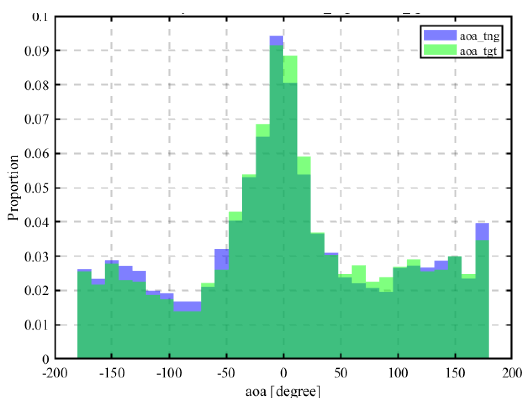
As shown in Figure 12, the target data does not significantly deviate from the training data, similar to the case of RSSI.
Figure 11.
AOA Training Data.
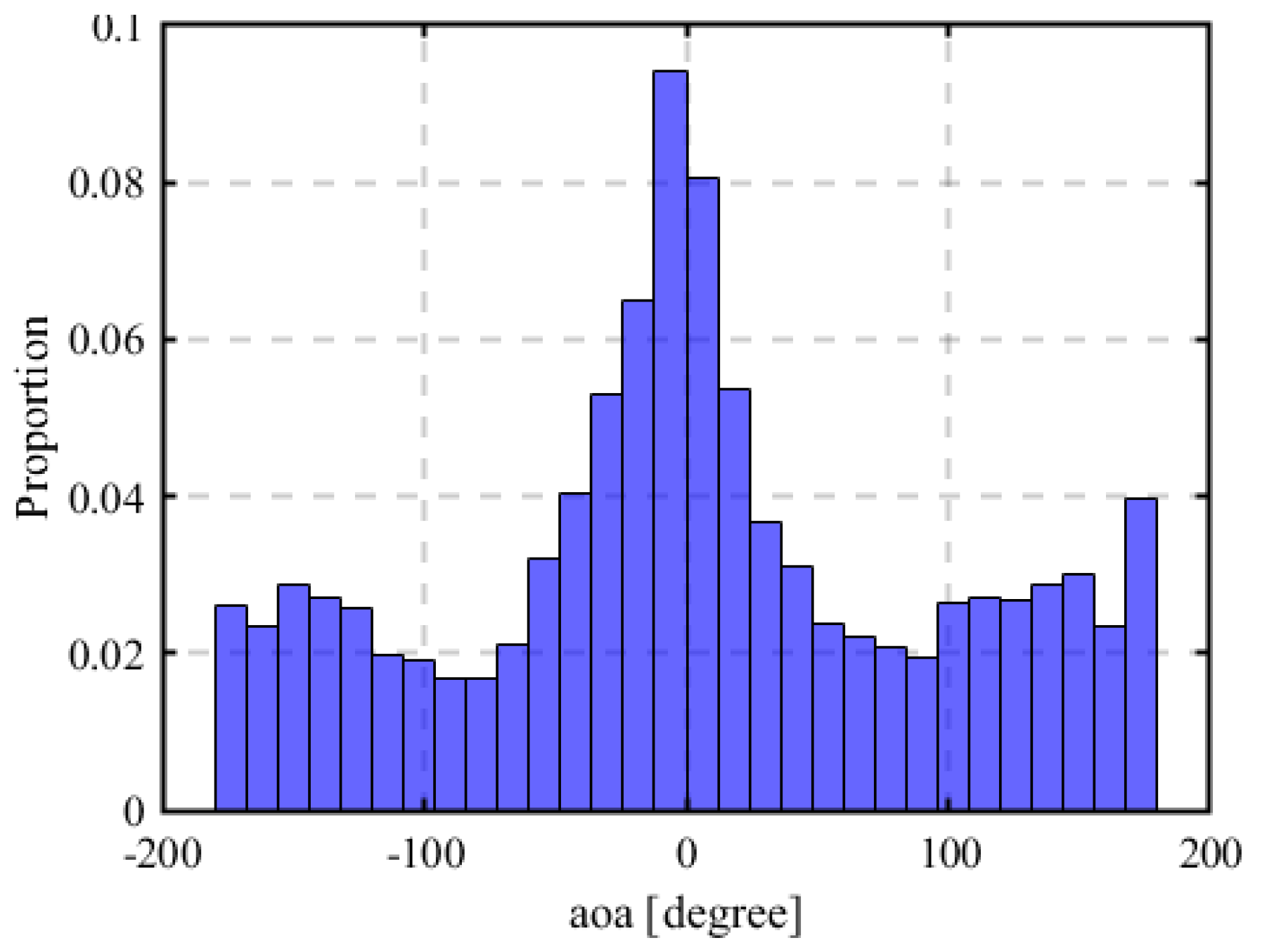
Figure 12.
Comparison of AOA Training and Target Data.
2.12. Estimation Using Elevation of Arrival (EOA)
For estimation using AOA, not only the azimuth angle but also the elevation angle (EOA: Elevation of Angle) is utilized. Figure 13 shows the training data for EOA, while Figure 14 presents the target data. Compared to RSSI and AOA, Figure 15 reveals that the target data does not significantly overlap with the training data. Possible reasons for this include the fact that the normal distribution model used for RSSI and AOA is not suitable for EOA, or that the target data distribution differs from the training data due to multipath effects. Additionally, in the ray-tracing simulation, the altitude was set up to 150 m, which may have made the elevation angle more susceptible to multipath effects.
When estimating with AOA, weights are assigned to AOA and EOA. In this study, AOA and EOA are weighted equally at 0.5 each. In the HYBRID model described later, the weighting coefficients for AOA and EOA are determined using linear interpolation. Therefore, for simplification, the estimation using AOA assigns equal weights of 0.5 to both RSSI and AOA.
2.13. HYBRID Model
The HYBRID model integrates the estimation process by assigning weights to RSSI, AOA, and EOA. First, the probability density function (PDF) values are computed using the mean and standard deviation of the training data for RSSI, AOA, and EOA. Using Equations (11), (12), and (13), the data is converted into dimensionless values. In these equations, represents the received data at the candidate Rx position, and denotes the fingerprint database.
Here,
Similarly, the probabilities for AOA and EOA are defined as:
where
For AOA and EOA, weight coefficients are determined through normalization using the standard deviation of the training data via linear interpolation. For RSSI, its weight coefficient is computed by subtracting the sum of AOA and EOA weights from a total weight value of 3. Using these weights, the probability is calculated as in Equation (14). By performing pattern matching to find the location with the highest probability, the source location is estimated.
2.14. Computation and Evaluation of Estimation Error
The root-mean-square error (RMSE) between the estimated coordinates and the actual radio source coordinates is computed as the Distance Error (DE). Given that and represent the estimated coordinates and the target coordinates, respectively, the distance error is computed using the norm as shown in Equation (15).
The distance error (DE) is computed for all 144 transmission sources.In this study, the computed DE is evaluated based on the mean value and the 90th percentile value of the cumulative distribution function (CDF) as key indicators of localization accuracy.The mean DE provides an overall estimate of the system’s accuracy, whereas the CDF 90% value assesses how frequently large errors (outliers) occur in localization results.
2.15. Sequential Estimation Model
In the previous models, the UAV’s trajectory is optimized to minimize the 90th percentile value of estimation error across all transmission sources. This essentially represents global learning.As will be discussed later in the results, estimation errors tend to be significantly degraded in highly obstructed environments, such as the southern area of the Ookayama campus. To address this, as illustrated in Figure 16, sequential learning is introduced to re-train areas that are prone to NLOS conditions. By iteratively updating the estimation model with NLOS-affected sources, this approach aims to enhance estimation accuracy in obstructed regions.
3. Results
3.1. Circular Trajectory Placement with a Radius of 100 m
Here, we analyze the localization results for different types of radio signal information with a radius of 100 meters. The primary reason for setting the radius to 100 meters is that it comprehensively covers the Ōokayama campus. Additionally, as will be discussed later, the results of localization with different radii Section 3.2 indicate that 100 meters is a reasonable choice for comparing different types of radio signal information. The results Section 3.2 show that when the radius is set to 100 meters, the localization accuracy of RSSI, AOA, and HYBRID is relatively unaffected by the radius.
The following Section 3.1.1-Section 3.1.3 discusses the localization results and the trends in estimation errors for each type of radio signal information.
3.1.1. Using Only RSSI
3.1.2. Using Only AOA
3.1.3. Hybrid
3.1.4. Discussion of the Results
The following Table 3 summarizes the mean estimation errors and the CDF 90% values for each type of radio signal information.Among the three combinations, the best localization performance was achieved with the HYBRID approach, followed by AOA, while RSSI yielded the worst results. Focusing on the CDF of the HYBRID approach, 90% of the sources are localized within an error of 10 m, demonstrating a faster convergence of the CDF compared to the other two methods. Examining the CDF of AOA, 90% of the sources are within an error of 20 m. Although the error distribution is not as poor as that of RSSI, some sources exhibit localization errors exceeding 30 m. Regarding the CDF of RSSI, 90% of the sources are within an error of 40 m. The presence of a larger number of sources with significant localization errors results in a slower convergence of the CDF.
3.2. Circular Trajectory Placement with Varying Radius
In the previous section, the radius was set to approximately 100 m, which comprehensively encompassed the campus. In this section, the radius was varied to investigate the dependence of localization errors on trajectory radius using RSSI and AOA. Simulations were conducted for five different trajectory radius: 50 m, 75 m, 100 m, 125 m, and 150 m. The results are shown in Figure 27, Figure 28 and Figure 29.
3.2.1. Discussion of the Result
As shown in Figure 27, an increasing trajectory radius in RSSI-based localization generally led to improved accuracy. However, at 150 m, the localization accuracy deteriorated, indicating that simply increasing the radius does not necessarily yield better results; instead, an optimal trajectory radius must be determined. One possible reason for the improved accuracy with increasing radius is that, in RSSI-based localization, reducing the radius decreases the Tx-Rx distance, leading to weaker signal attenuation. As a result, noise has a greater impact, causing degradation in localization accuracy. On the other hand, Figure 28 shows that AOA-based localization exhibited low sensitivity to trajectory radius. This suggests that increasing the radius does not contribute to reducing angular estimation errors.
3.3. Sequential Estimation
3.3.1. Results for the First Estimation Using RSSI
The cumulative distribution function (CDF) summarizing the results of the second estimation using RSSI, AOA, and HYBRID after the first estimation with RSSI is shown in Figure 30. The figure indicates that using AOA or HYBRID for the second estimation leads to faster CDF convergence and higher localization accuracy compared to using RSSI for both estimations.Similar to the first estimation, using RSSI for the second estimation results in a larger number of significant outliers with high localization errors. This suggests that the second estimation was not sufficient to correct these large errors.
When HYBRID is applied with a strong weighting toward RSSI, the RSSI → HYBRID approach improves accuracy compared to RSSI → RSSI. However, it still includes some sources with large localization errors.
3.3.2. Results for the First Estimation Using AOA
The results of the first estimation using AOA are shown in Figure 31. Among the three scenarios, the best localization accuracy was achieved with AOA → HYBRID.In all three scenarios, there was no significant difference in the median localization error. This indicates that for nearly half of the sources, the choice of Sequential estimation method had little impact on localization accuracy. However, the HYBRID approach resulted in a greater number of sources with high localization accuracy. This suggests that the inclusion of RSSI in the HYBRID approach allowed for the incorporation of distance information, leading to improved localization performance. On the other hand, around the CDF 90% region, there was no substantial difference between AOA → RSSI and AOA → HYBRID. This implies that the weighting effect in the HYBRID approach had a limited impact on sources with very large localization errors. Furthermore, when RSSI was used for Sequential optimization, the prominent outliers observed in the first estimation were no longer present, resulting in improved localization accuracy.
3.3.3. Results for the First Estimation Using HYBRID
The results of the first estimation using HYBRID are shown in Figure 32. Among the three scenarios, the highest localization accuracy was achieved with HYBRID → HYBRID. In terms of the median localization error (CDF 50%), HYBRID → HYBRID exhibited the highest accuracy. However, around the CDF 90% region, there was no significant difference between HYBRID → HYBRID and HYBRID → RSSI. This suggests that while using HYBRID for the second estimation improves accuracy for a larger number of sources, the occurrence rate of sources with large localization errors remains comparable to that of using RSSI for the second estimation. In other words, when HYBRID is used in the first estimation, the degree of localization error improvement through Sequential estimation may be limited.
4. Conclusions
In this study, we investigated the improvement of source localization accuracy using different radio wave information: RSSI, AOA, EOA, and a hybrid approach that integrates these parameters. The results confirmed that the hybrid approach achieved the highest accuracy, and the accuracy was further improved by applying sequential optimization. In the sequential optimization process, the extent of accuracy improvement varied depending on the type of radio wave information used for the initial estimation. Particularly, when RSSI was used for the initial estimation, significant accuracy improvement was observed when AOA or the hybrid approach was applied for the sequential optimization. On the other hand, when AOA or the hybrid approach was used initially, while improvements were confirmed for 15 transmission sources, the overall improvement was limited. These findings suggest that by appropriately combining different radio wave information and applying sequential optimization, the accuracy of source localization can be enhanced. Future challenges include applying the method to sources with unknown frequency bands in real-world environments, developing further optimization techniques, and implementing cooperative estimation using multiple units.
References
- Ministry of Internal Affairs and Communications, Japan. Latest Trends in Radio Policy. Available online: https://www.soumu.go.jp/main_content/000932571.pdf (accessed on 17 March 2025).
- Ministry of Internal Affairs and Communications, Japan. Overview of Illegal Radio Station Countermeasures. Available online: https://www.tele.soumu.go.jp/j/adm/monitoring/summary/ad_pro/index.htm (accessed on 17 March 2025).
- Ministry of Internal Affairs and Communications, Japan. Radio License Information System. Available online: https://www.soumu.go.jp/soutsu/kanto/re/system/ (accessed on 17 March 2025).
- Tanaka, S. Study on Sensor Placement for Outdoor Radio Source Localization Using UAVs. Master’s thesis, Tokyo Institute of Technology, 2020.
- Kamei, T. Investigation on Outdoor Positioning Using Fingerprinting Method and UAV Flight Path Optimization. Master’s thesis, Tokyo Institute of Technology, 2022.
- Tan, J.; Zhao, H. UAV Localization with Multipath Fingerprints and Machine Learning in Urban NLOS Scenario. In Proceedings of the 2020 IEEE 6th International Conference on Computer and Communications (ICCC). IEEE, 2020, pp.1551–1557. [CrossRef]
- Zhou, L.; Ning, X.; You, M.Y.; et al. Robust Multi-UAV Placement Optimization for AOA-Based Cooperative Localization. IEEE Transactions on Intelligent Vehicles 2024, pp. 1–15. Early Access. [CrossRef]
- Haniz, A.; Tran, G.K.; Sakaguchi, K.; et al. Hybrid Fingerprint-based Localization of Unknown Radios: Measurements in an Open Field. In Proceedings of the 2017 IEEE Asia Pacific Microwave Conference (APMC). IEEE, November 2017, pp. 967–970. [CrossRef]
- Murata, S.; Matsuda, T.; Hiraguri, T. Multiple-wave source localization using UAVs in NLOS environments. IEICE Communications Express (ComEX) 2020, 13, 375–378. [Google Scholar] [CrossRef]
- Holis, J.; Pechac, P. Elevation Dependent Shadowing Model for Mobile Communications via High Altitude Platforms in Built-up Areas. IEEE Transactions on Antennas and Propagation 2008, 56, 1078–1084. [Google Scholar] [CrossRef]
- Zhang, R.; Lu, X.; Zhao, J.; Cai, L.; Wang, J. Measurement and Modeling of Angular Spreads of Three-Dimensional Urban Street Radio Channels. IEEE Transactions on Vehicular Technology 2017, 66, 3555–3570. [Google Scholar] [CrossRef]
- Thomas, T.; Vook, F.; Mellios, E.; et al. 3D Extension of the 3GPP/ITU Channel Model. In Proceedings of the IEEE Vehicular Technology Conference (VTC Spring), 2013, pp. 1–5. [CrossRef]
- Gu, Y.; Lo, B.P.L.; Meng.; et al. Wi-Fi Fingerprint-Based Indoor Positioning: Recent Advances and Comparisons. IEEE Communications Surveys & Tutorials 2015, 18, 466–490. [CrossRef]
- Ladd, A.M.; Bekris.; et al. A Survey of Indoor Positioning Systems for Wireless Personal Networks. IEEE Communications Surveys & Tutorials 2009, 11, 58–78. [CrossRef]
- Azari, A.; Ghavimi, F.; et al. Machine Learning assisted Handover and Resource Management for Cellular-Connected Drones 2019. [CrossRef]
- Kennedy, J.; Eberhart, R. Particle Swarm Optimization. In Proceedings of the IEEE International Conference on Neural Networks, 1995, Vol. 4, pp. 1942–1948. [CrossRef]
- Shimizu, Y. Introduction to Optimization Engineering: A Smart Decision-Making Workbench; Corona Publishing Co., 2010.
- Fujita, N.; Chauvet, N.; Röhm, A.; et al. Efficient Pairing in Unknown Environments: Minimal Observations and TSP-Based Optimization. IEEE Access 2022, 10, 57630–57640. [Google Scholar] [CrossRef]
Figure 1.
Trends in the number of illegal radio stations and regulatory measures (adapted from [2] ).
Figure 1.
Trends in the number of illegal radio stations and regulatory measures (adapted from [2] ).
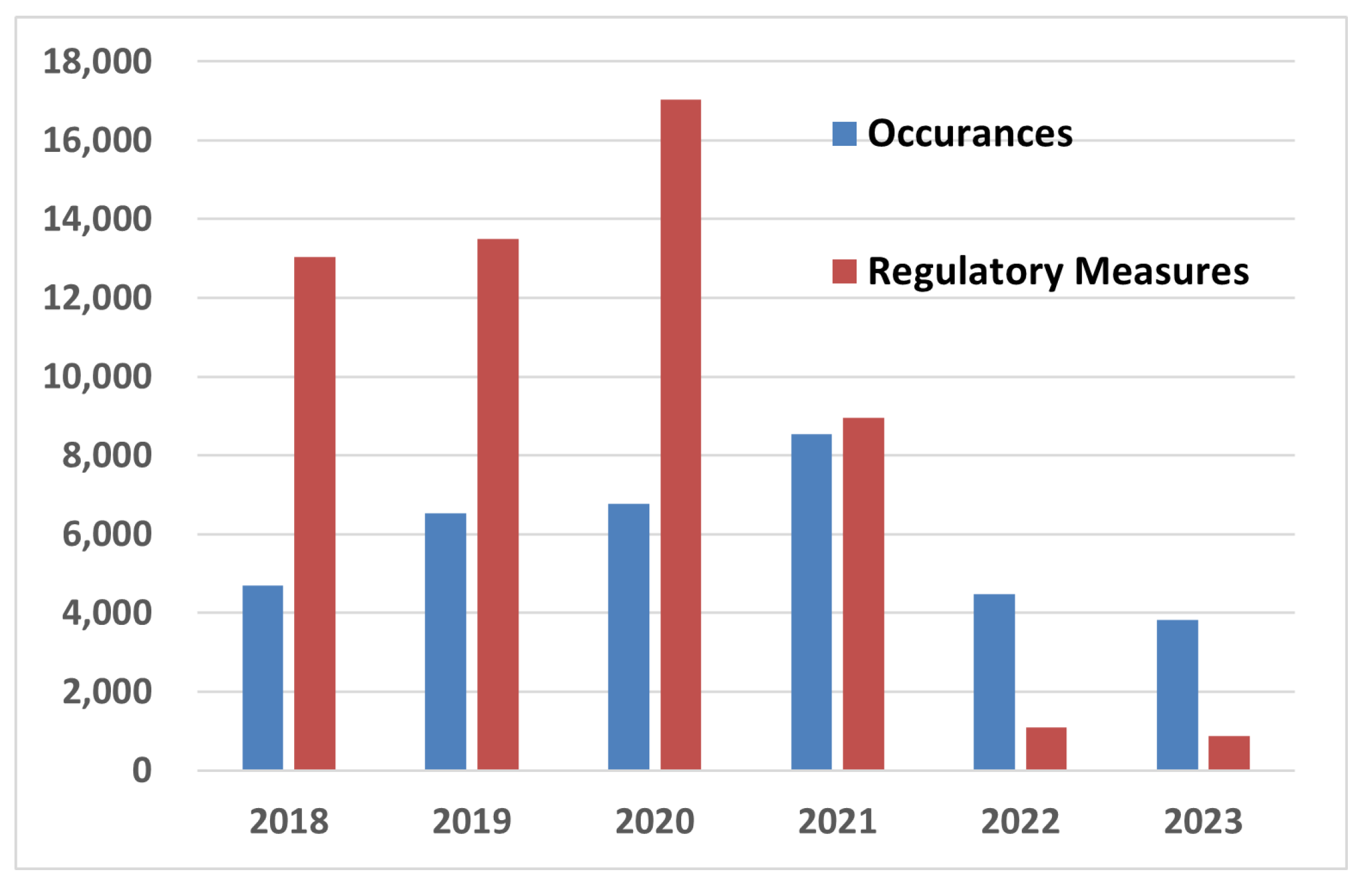
Figure 2.
Concept of the DEURAS System (adapted from [3] ).
Figure 2.
Concept of the DEURAS System (adapted from [3] ).
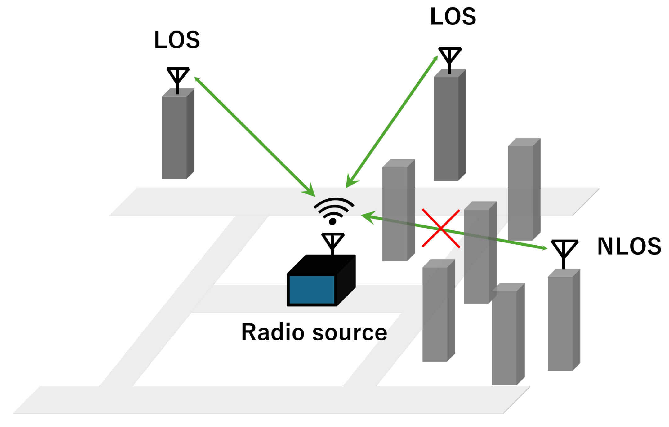
Figure 4.
Simulation terrain model.
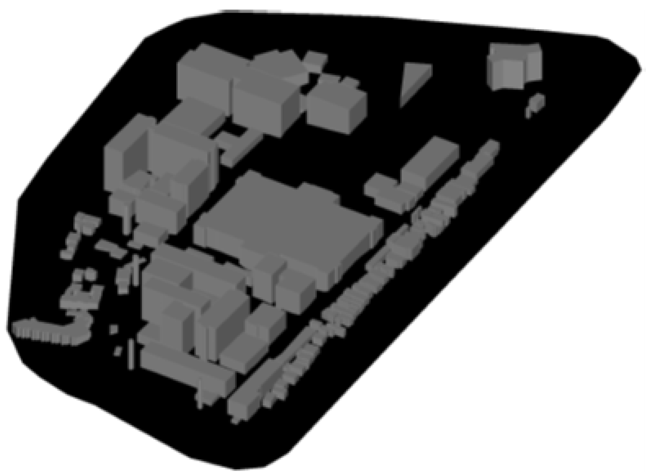
Figure 5.
Layout of transmitters and candidate sensor points.
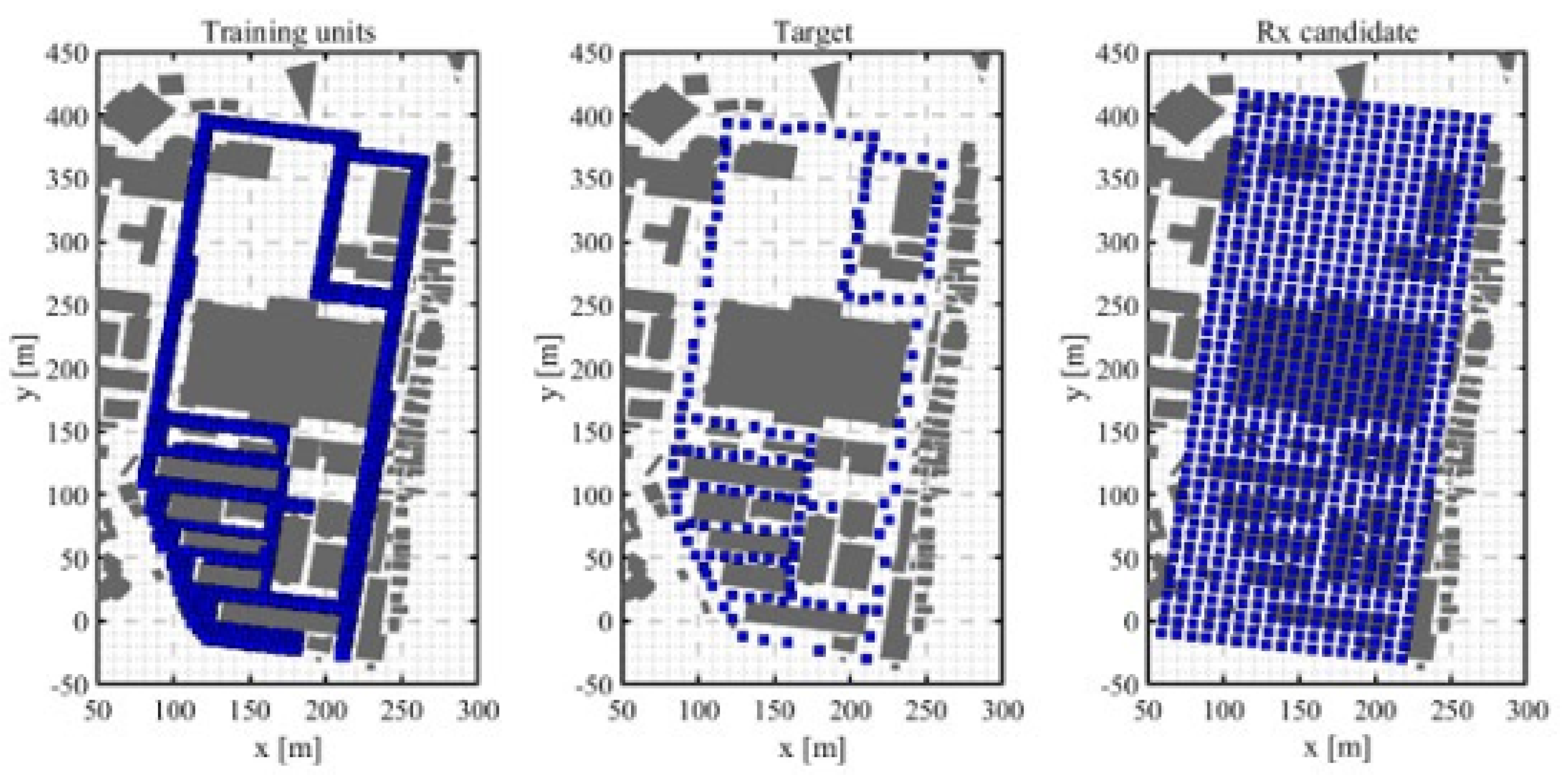
Figure 6.
Candidate receiver antenna positions at an altitude of 50 m and transmitter placement.
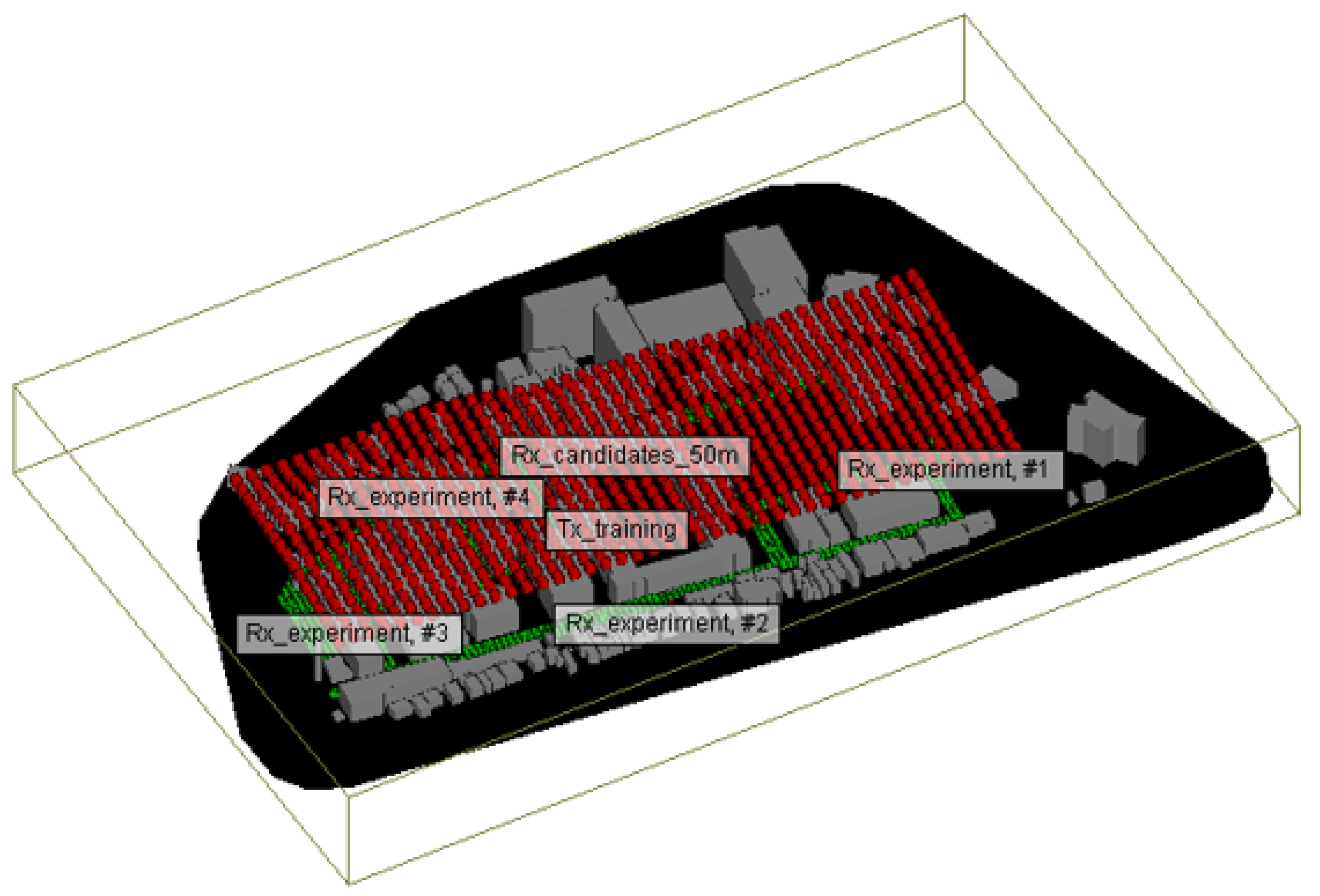
Figure 7.
LoS Probability Calculation Model.
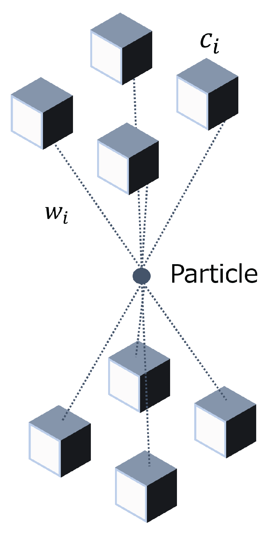
Figure 8.
Circular UAV Orbit (8 Sampling Points).
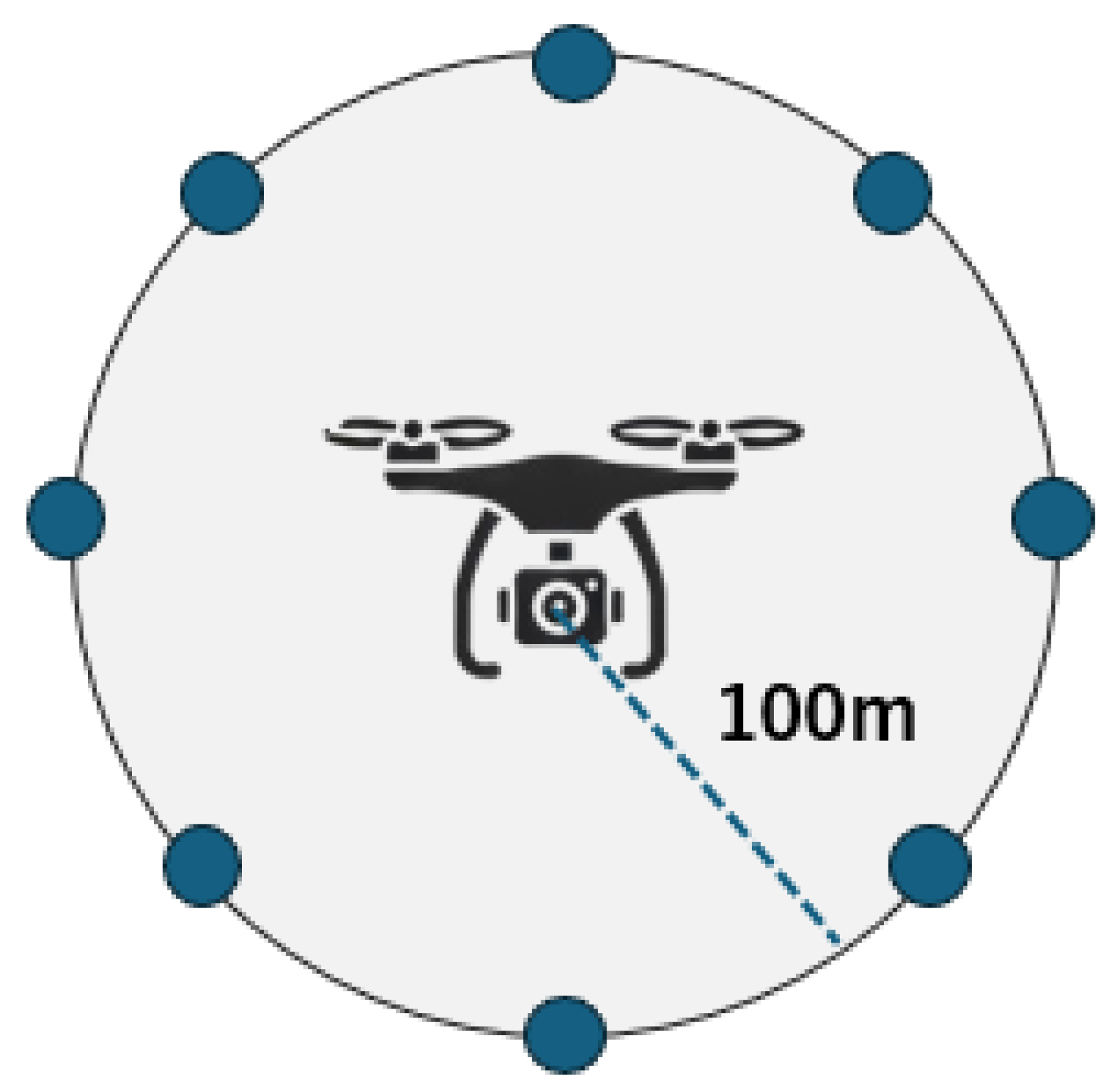
Figure 9.
RSSI Training Data.
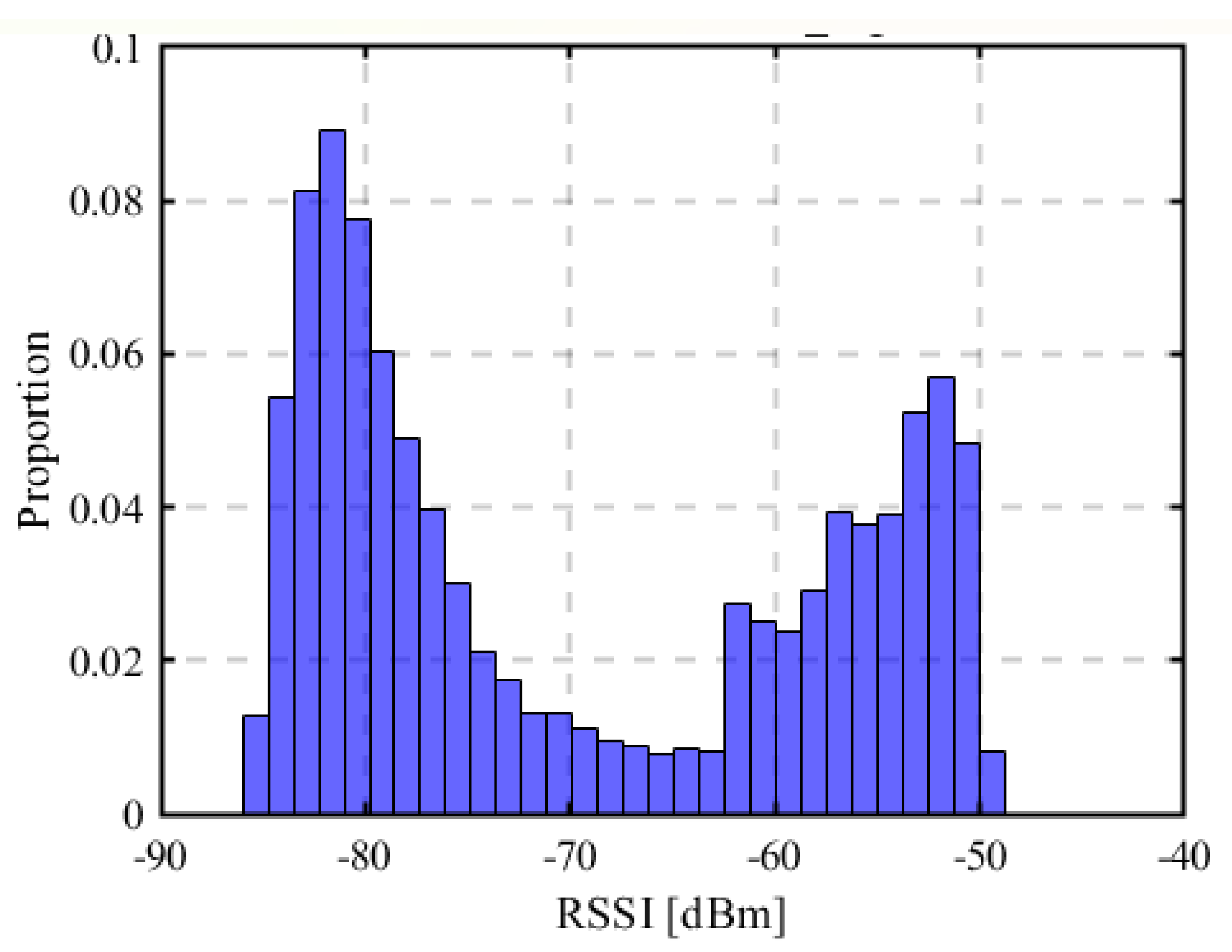
Figure 10.
Comparison of RSSI Training and Target Data.
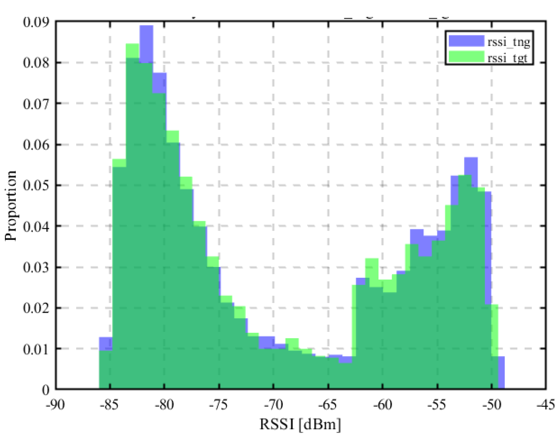
Figure 13.
EOA Training Data.
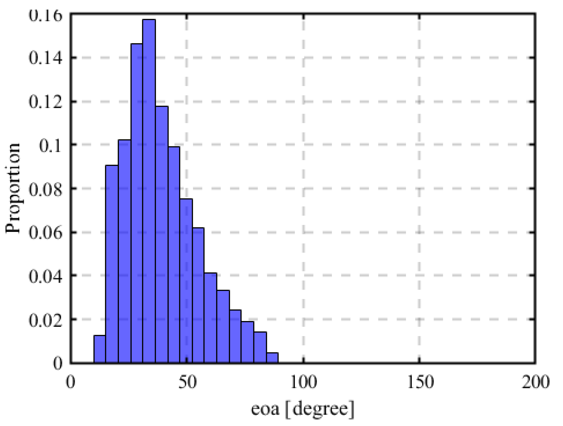
Figure 14.
EOA Target Data.
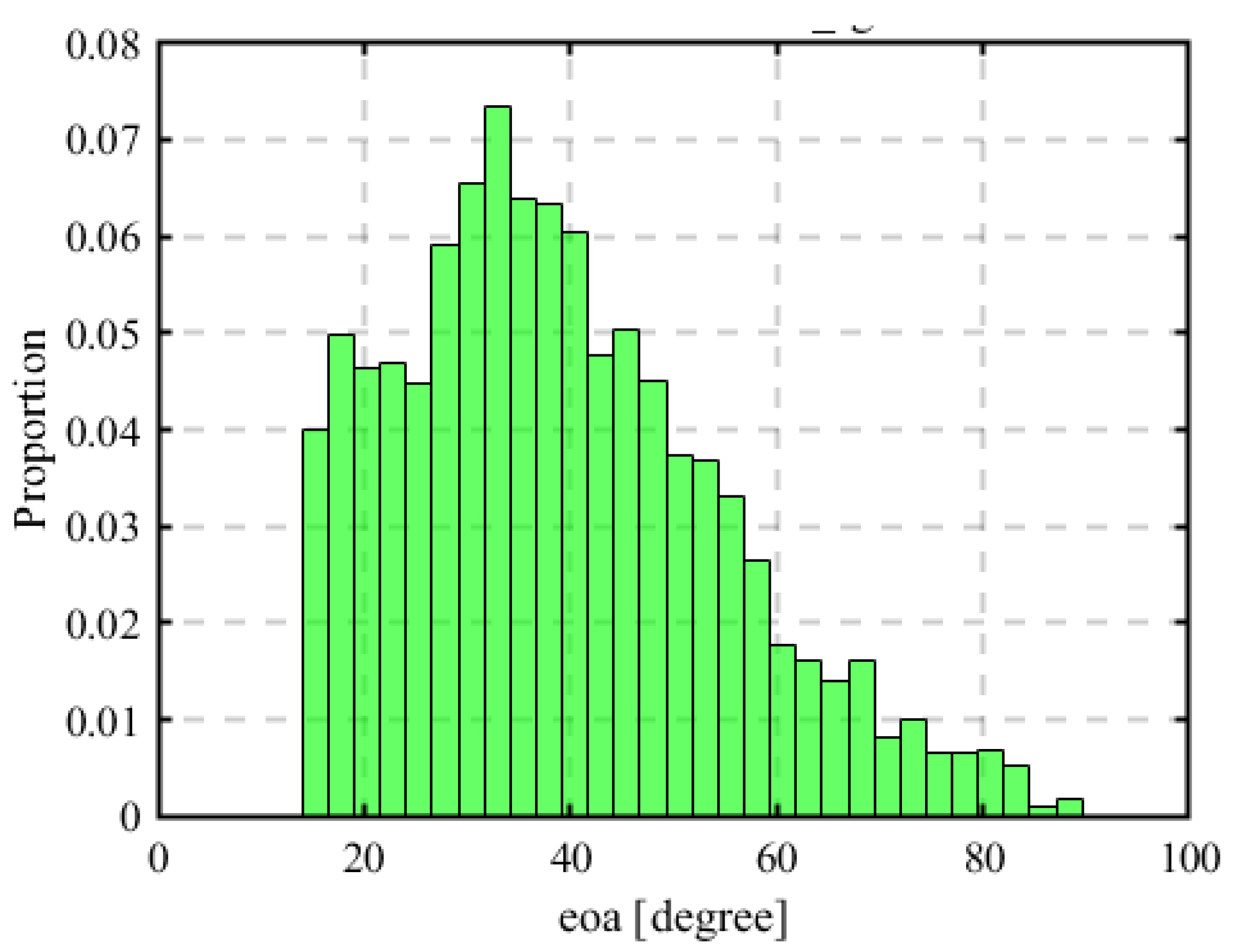
Figure 15.
Comparison of EOA Training and Target Data.
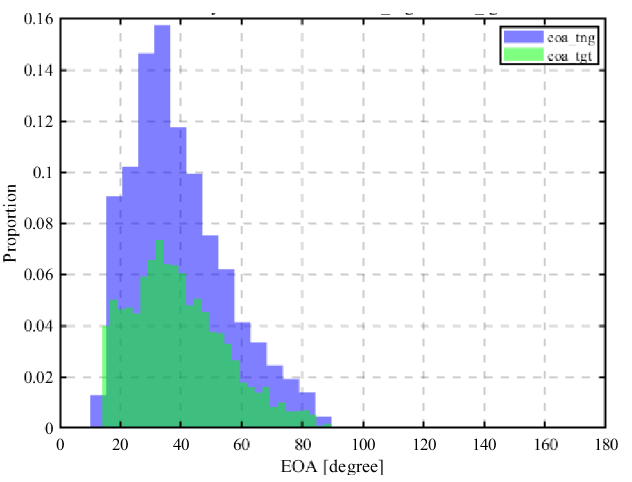
Figure 16.
Sequential Estimation.
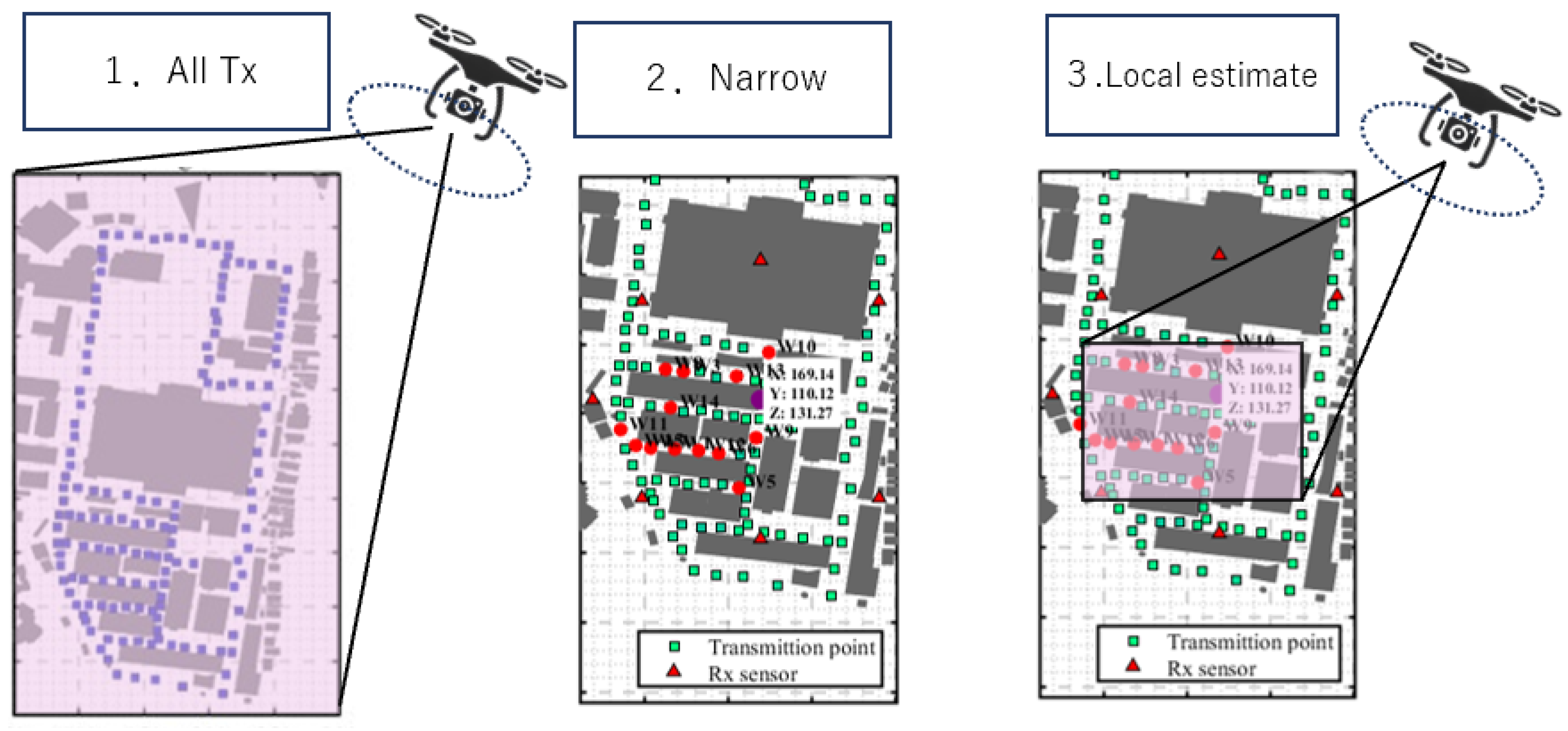
Figure 17.
Optimized placement, including UAV altitude.
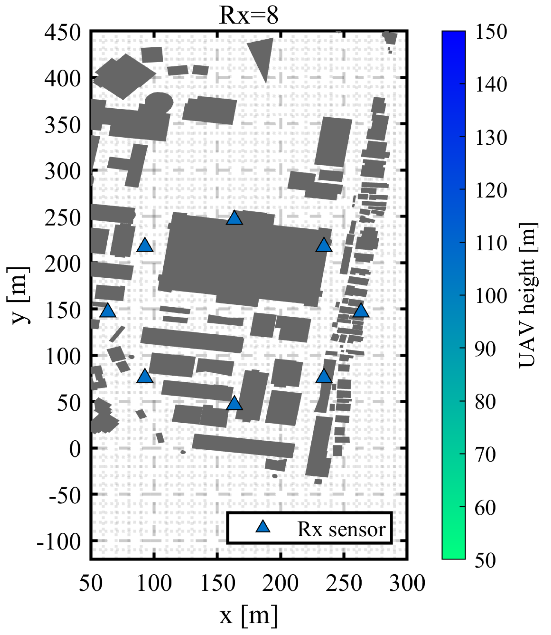
Figure 18.
Distribution of localization errors relative to the source.
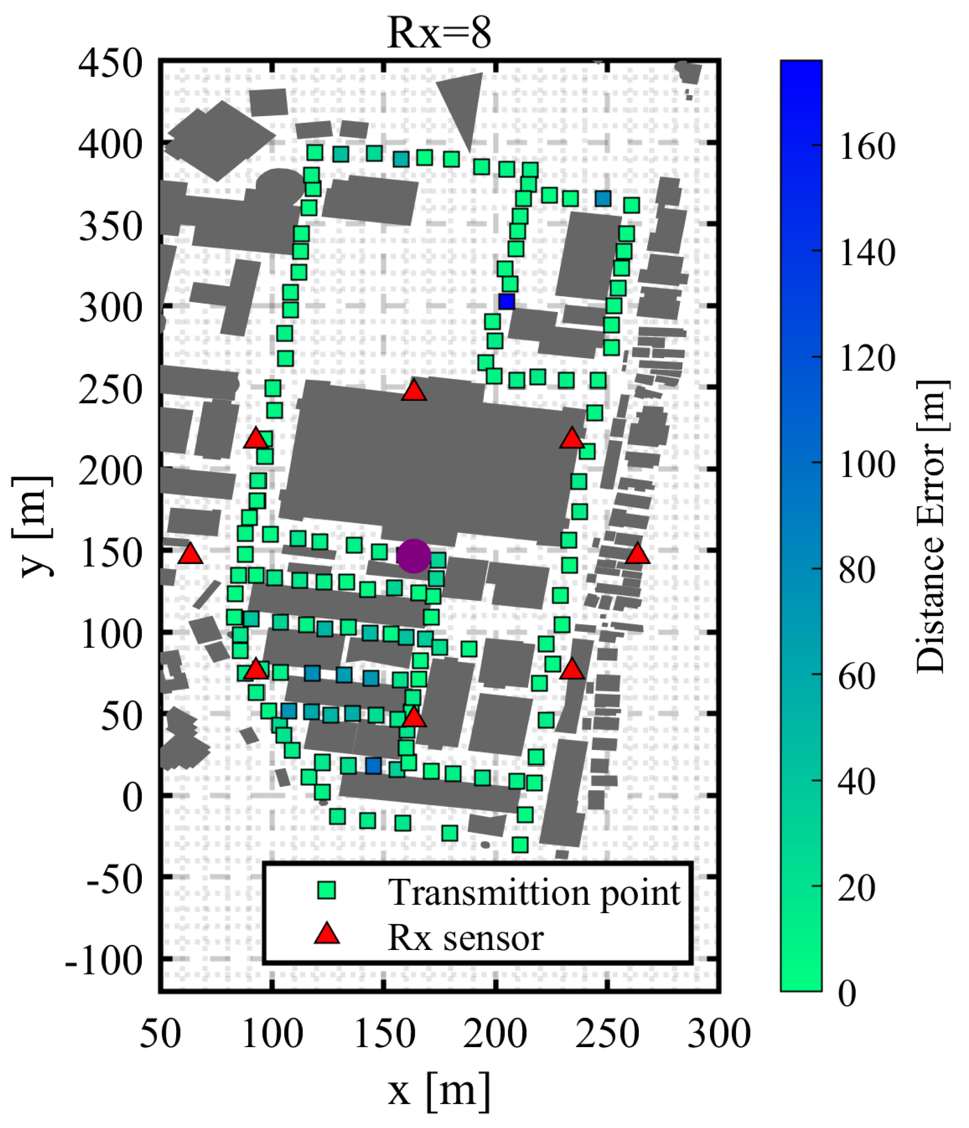
Figure 19.
Cumulative distribution function of localization errors.
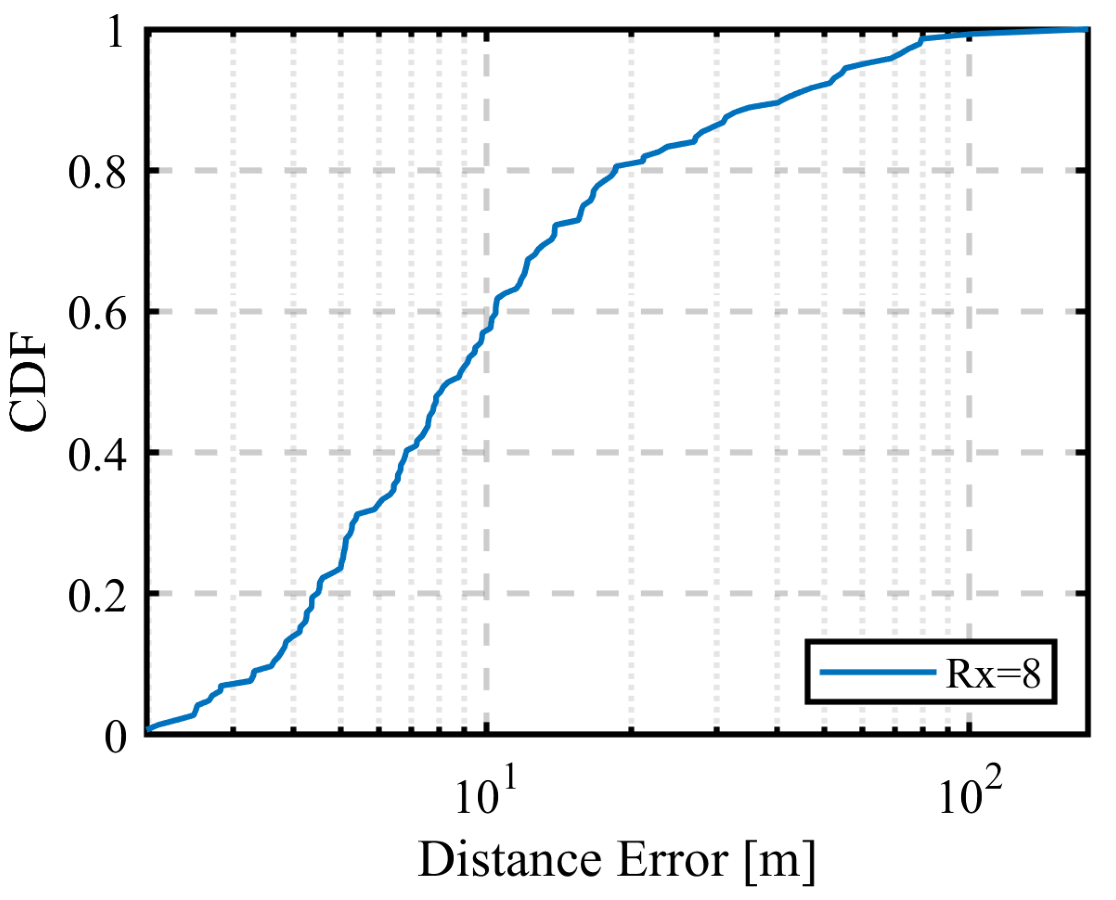
Figure 20.
Optimized placement, including UAV altitude.

Figure 21.
Distribution of localization errors relative to the source.

Figure 22.
Cumulative distribution function of localization errors.
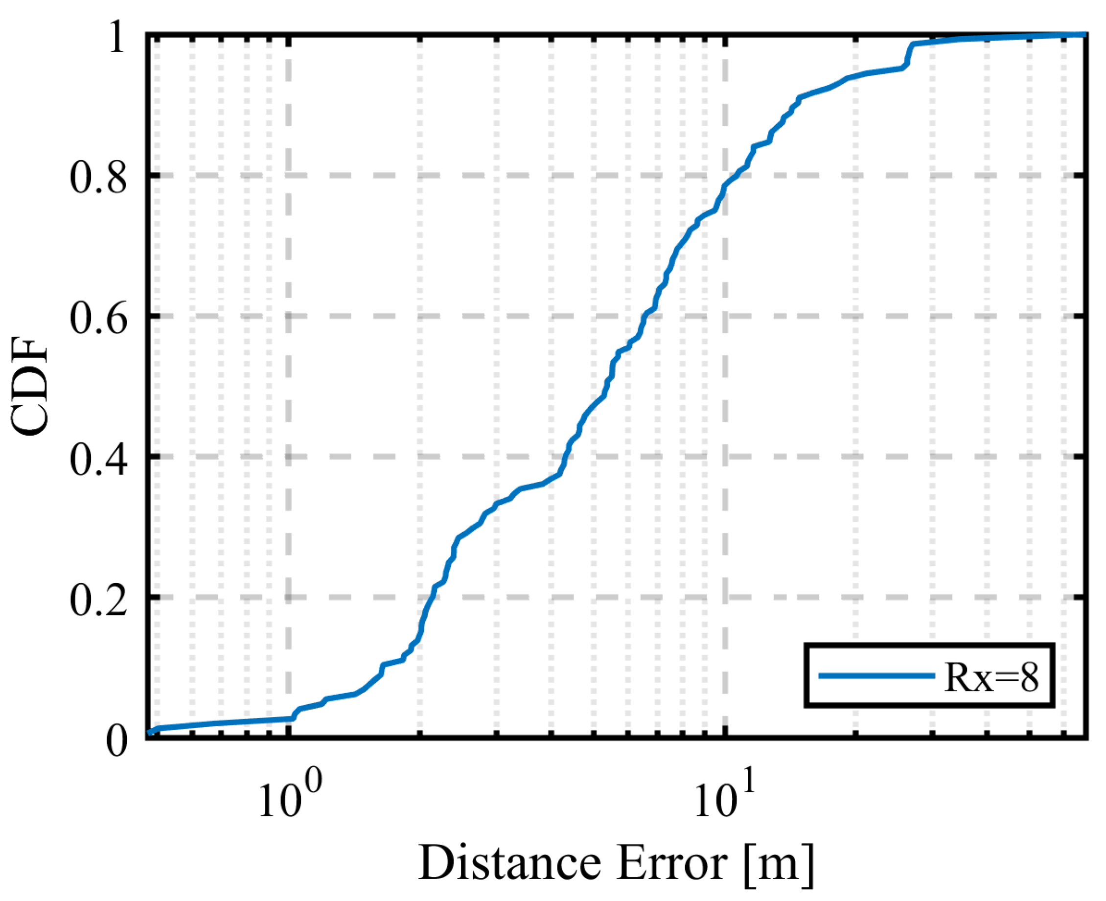
Figure 23.
Optimized placement, including UAV altitude.

Figure 24.
Distribution of localization errors relative to the source.
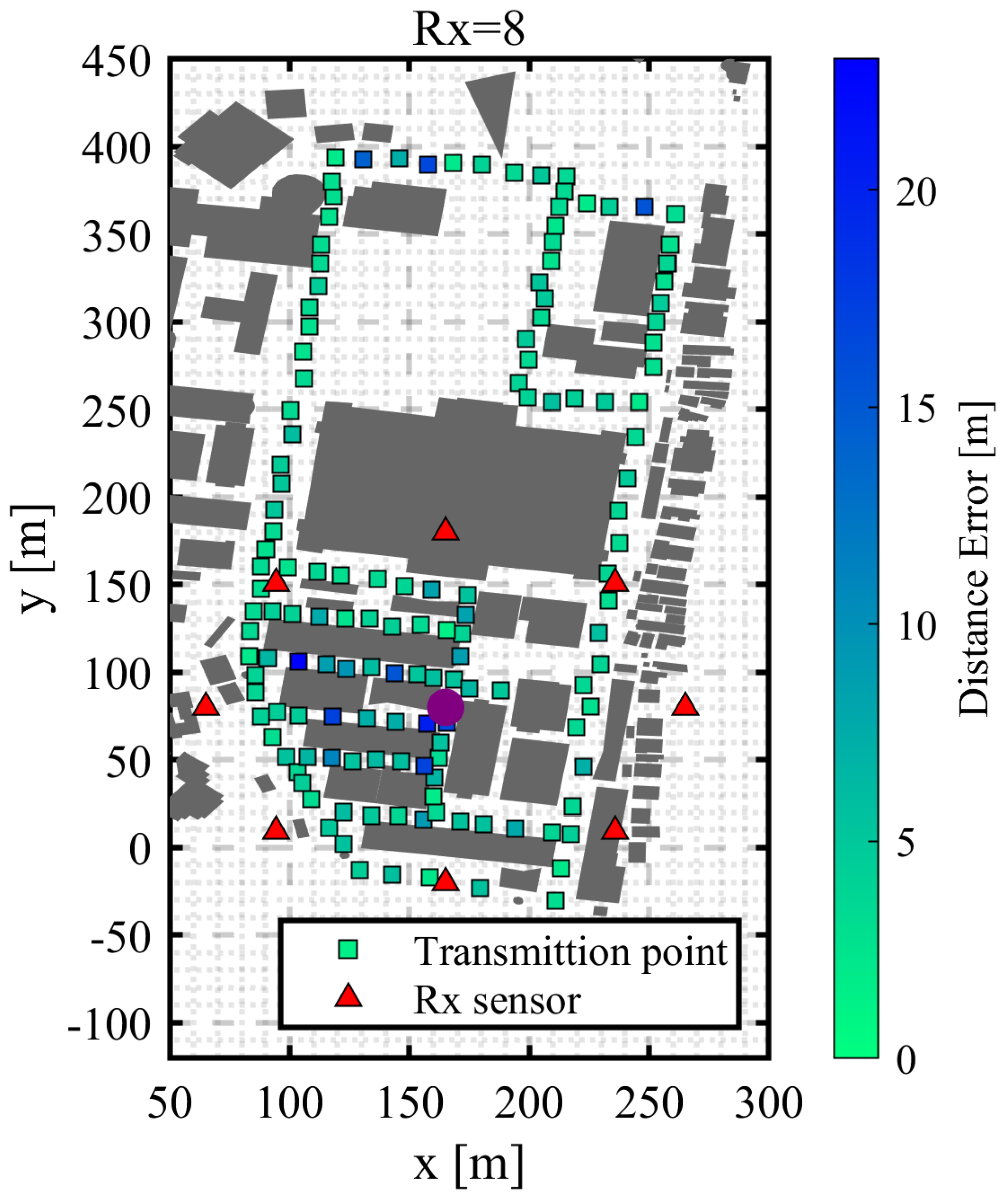
Figure 25.
Cumulative distribution function of localization errors.
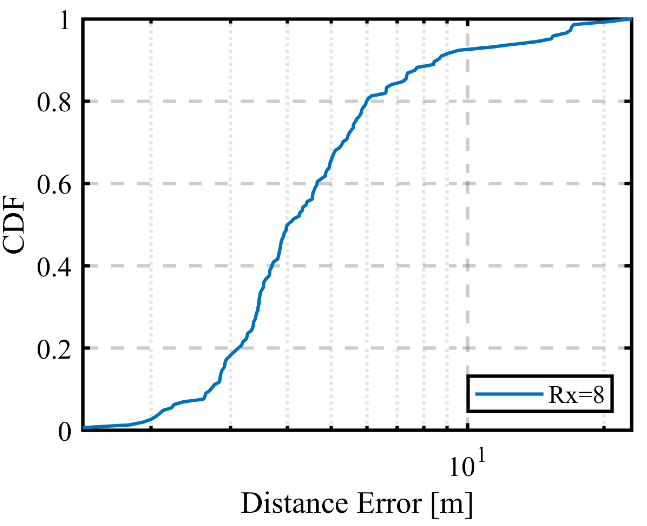
Figure 26.
CDF of localization errors for different radio signal information.
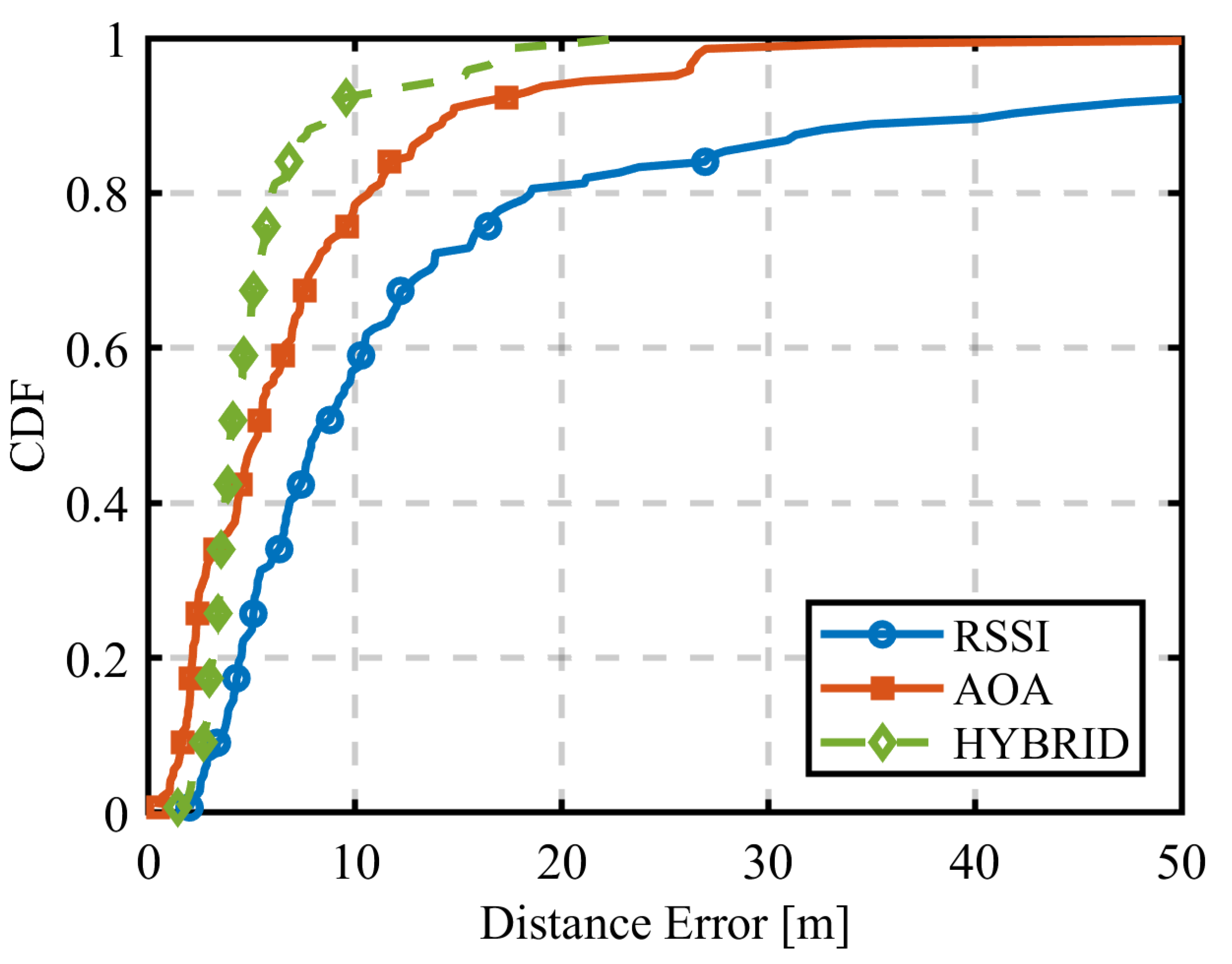
Figure 27.
Localization results with varying radius using RSSI.
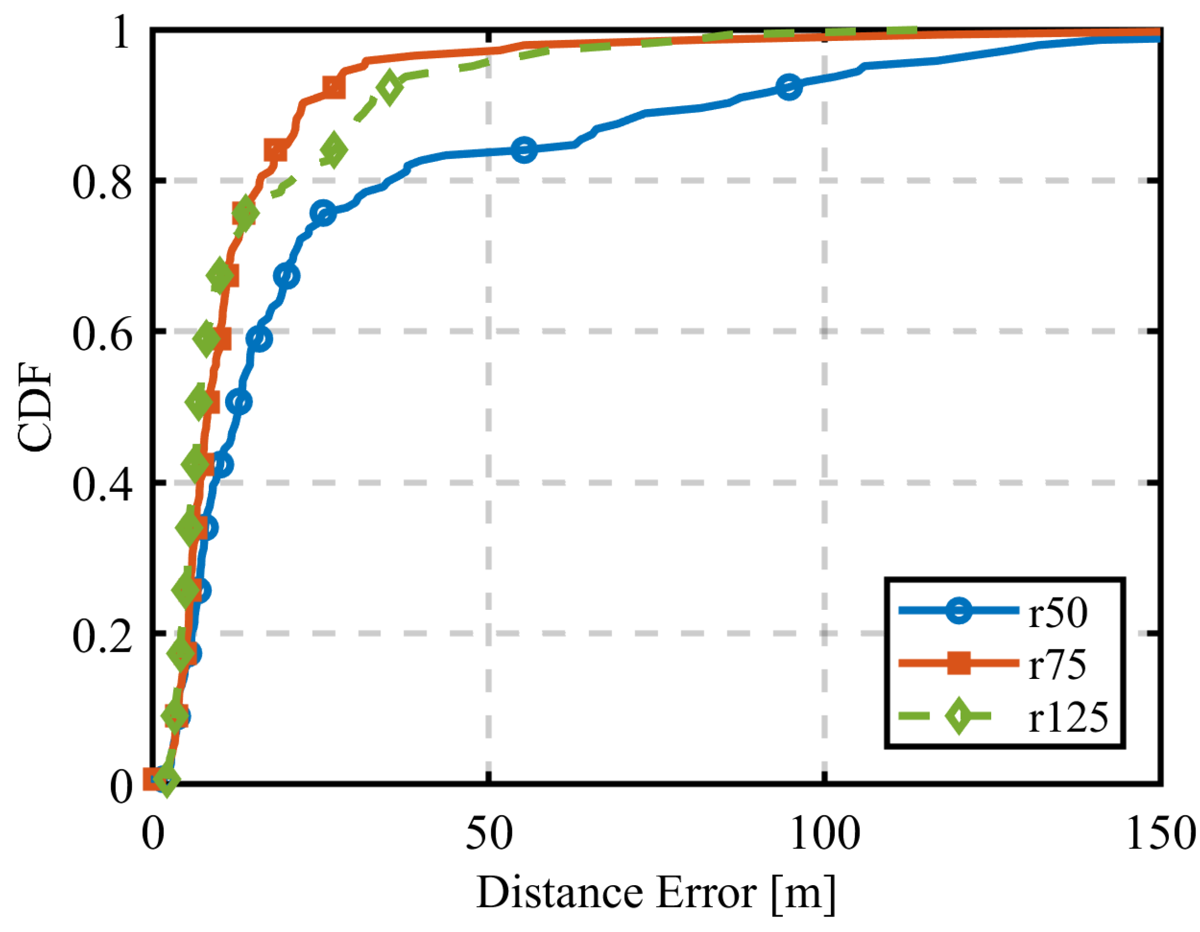
Figure 28.
Localization results with varying radius using AOA.
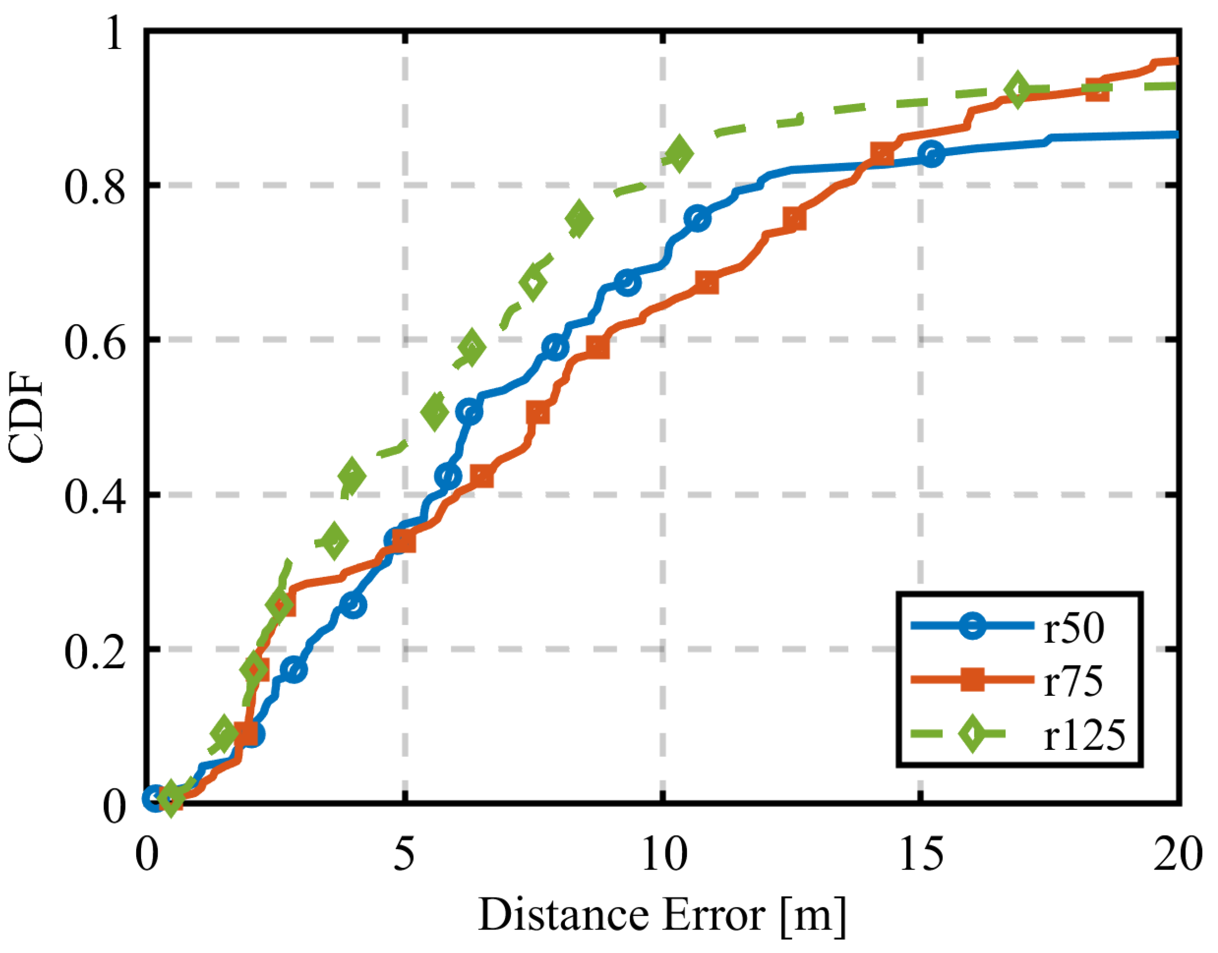
Figure 29.
Localization results with varying radius using the HYBRID approach.
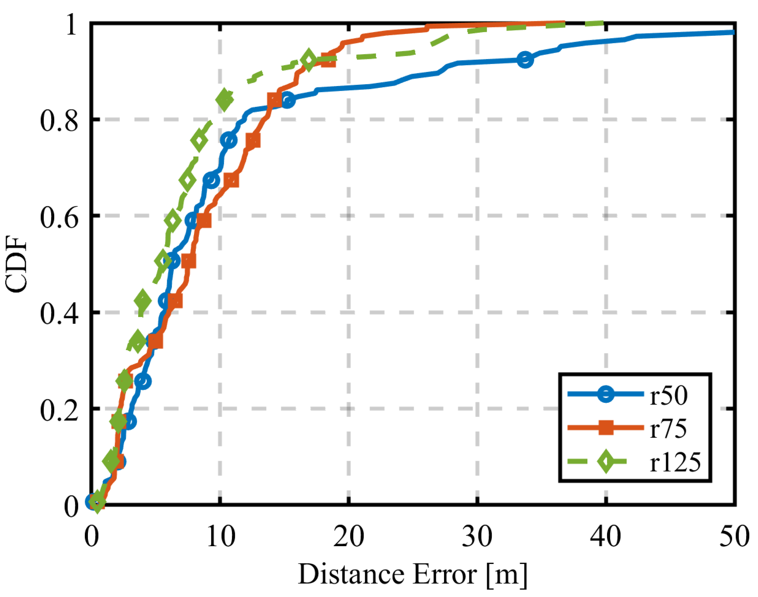
Figure 30.
Sequential estimation scenarios when the first estimation is performed using RSSI.
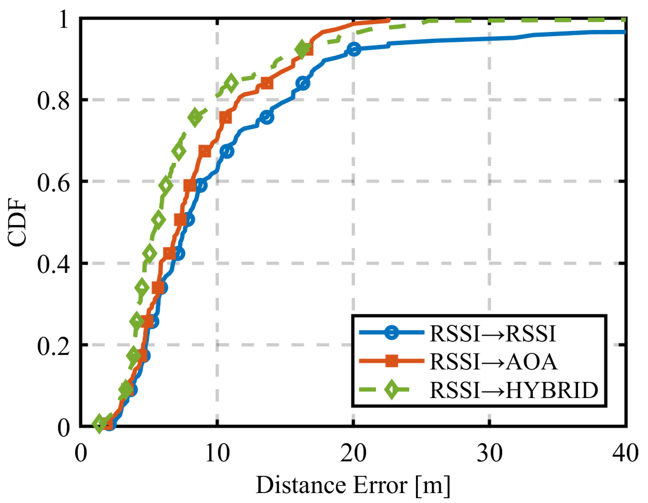
Figure 31.
Sequential estimation scenarios when the first estimation is performed using AOA.
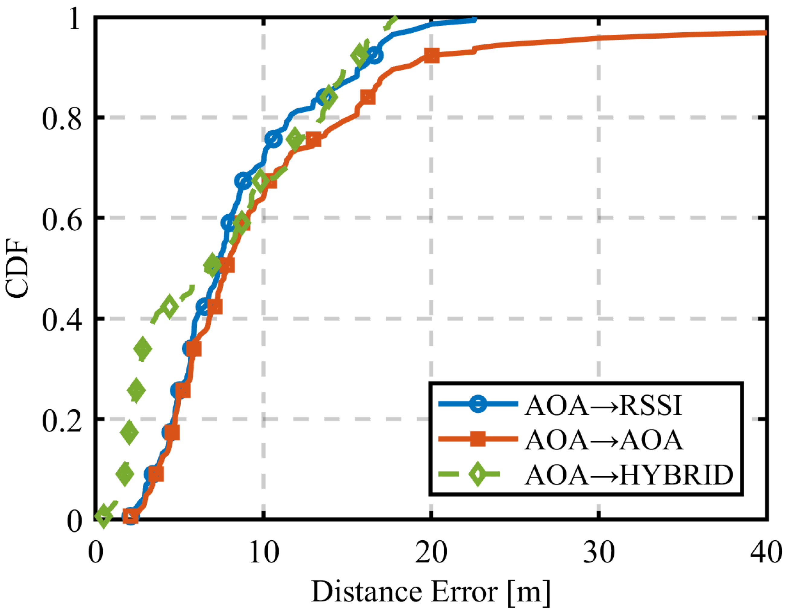
Figure 32.
Sequential estimation scenarios when the first estimation is performed using HYBRID.
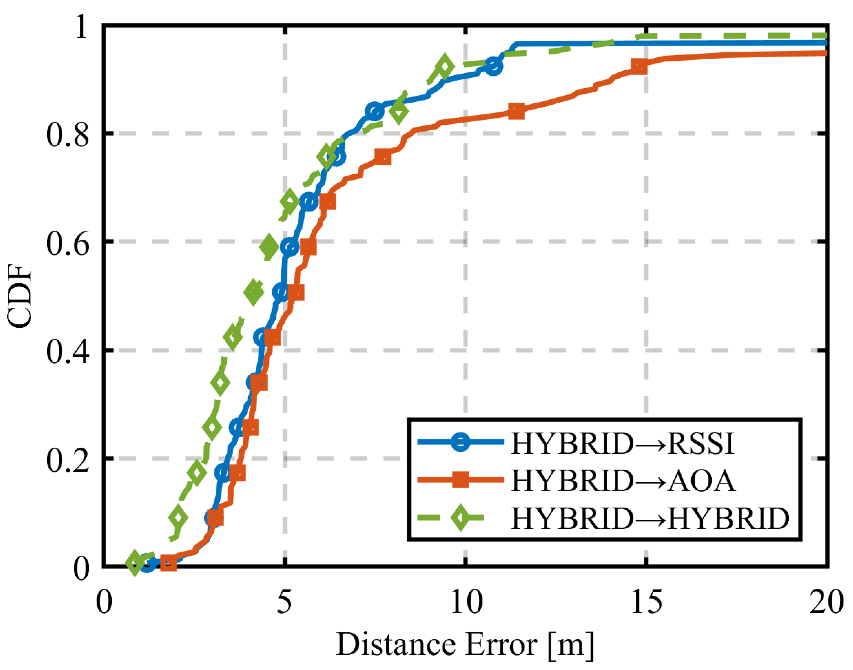

Table 1.
Ray-Tracing Parameters.
| Item | Value |
|---|---|
| Model | 3D (Ray launching) |
| Frequency [GHz] | 2.487 |
| Bandwidth [MHz] | 5.00 |
| Number of Reflections | 6 |
| Number of Diffractions | 1 |
| Number of Transmissions | 0 |
| Rx | Antenna Type: Isotropic |
| Height [m]: 50/75/100/125/150 | |
| Antenna Gain [dBi]: 2.0 | |
| Tx | Antenna Type: Isotropic |
| Transmission Power [dBm]: 27 |
Table 2.
PSO Parameters Used in This Study.
| Initial position , Initial velocity | |
|---|---|
| w | 0.5 |
| Number of particles | 100 |
| 10 |
Table 3.
Mean localization errors and CDF 90% values.
| Radio Signal Information | Mean Error [m] | CDF 90% Value [m] |
|---|---|---|
| RSSI | 16.4 | 41.9 |
| AOA | 7.5 | 14.8 |
| HYBRID | 5.3 | 8.7 |
Disclaimer/Publisher’s Note: The statements, opinions and data contained in all publications are solely those of the individual author(s) and contributor(s) and not of MDPI and/or the editor(s). MDPI and/or the editor(s) disclaim responsibility for any injury to people or property resulting from any ideas, methods, instructions or products referred to in the content. |
© 2025 by the authors. Licensee MDPI, Basel, Switzerland. This article is an open access article distributed under the terms and conditions of the Creative Commons Attribution (CC BY) license (http://creativecommons.org/licenses/by/4.0/).
Copyright: This open access article is published under a Creative Commons CC BY 4.0 license, which permit the free download, distribution, and reuse, provided that the author and preprint are cited in any reuse.


