
Submitted:
08 April 2025
Posted:
09 April 2025
You are already at the latest version
Abstract
This study presents the results of an investigation into the potential use of the DiagBelt+ magnetic diagnostic system for assessing the quality of conveyor belt splices. Splices in conveyor belts are susceptible to damage and irregularities resulting from assembly errors, improper vulcanization parameters, or unfavorable operational conditions. Detecting geometric deviations from the reference standard after splice fabrication can serve as a component of QA/QC systems. Later deviations may indicate material or fabrication defects. To date, applications of the DiagBelt+ system have been limited to locating damage within the belt and its splices. Recently, efforts have been made to extend the system’s functionality to include splice diagnostics. The study was conducted under laboratory conditions on an ST2500 belt featuring five splices (three bias and two straight splices). Data acquisition was performed under various configurations of measurement parameters, including sensor-to-belt distance, belt travel speed, and system sensitivity threshold. For each splice, the signal width was measured and analyzed as a potential indicator of splice geometry and quality. The results indicate that the DiagBelt+ system can be effectively used for splice diagnostics. Work has commenced on automating the splice quality assessment process.
Keywords:
conveyor belt splices
; non-invasive diagnostics
; conveyor belts
; DiagBelt+
1. Wprowadzenie
Belt conveyors are widely used for the transportation of bulk materials and raw resources[1,2]. They are employed across numerous industrial sectors, including open-pit and underground mining, metallurgy, cement plants, factories, and ports. Their widespread adoption is primarily due to their relatively simple construction, high reliability, and capability to operate in environments where alternative transport methods are either impractical or impossible. However, the use of conveyors is accompanied by a range of operational challenges. Continuous efforts are made to develop new solutions aimed at achieving a fully automated transport system, in line with the principles of Industry 4.0 [3,4,5].
One of the most failure-prone components of a conveyor system is the conveyor belt itself, which is in direct contact with the transported material and therefore vulnerable to damage. Belt wear processes can be divided into natural, cumulative wear caused by friction and bending (such as edge and cover abrasion, and core fatigue) and random, sudden events like belt cuts, punctures, and breakages [6,7,8,9]. A typical conveyor belt consists of three layers :
- Top cover, which protects the core from damage caused by falling material and abrasive forces during loading and transport;
- Core, which transmits longitudinal forces required for moving large masses of material and allows the belt to flex into a trough shape;
- Bottom cover, which protects the core from wear due to contact with pulleys and idlers along the conveyor route.
Depending on the materials used in the core layer, conveyor belts are categorized as either textile-reinforced or steel cord-reinforced. Figure 1 illustrates the structural schematics of both types.
Conveyor belts are assembled into a closed loop from multiple sections, which are delivered to the installation site on reels. Due to transportation constraints (maximum permissible weight and reel diameter), individual sections typically cannot exceed several hundred meters in length [10]. These sections must be spliced to form a durable loop capable of fulfilling the required transport function. At the splice location, the belt core loses its continuity over a short region, making the splice the weakest link in the series-structured loop. An example of such a closed conveyor belt loop is shown in Figure 2.
To ensure the required strength and fatigue resistance, standards have been developed for belt splicing (e.g., PN-C-94147:1997, EN-ISO-1120:2012). Textile-reinforced belts may be joined using hot vulcanization, cold bonding/welding, or mechanical fasteners, while steel cord belts are exclusively joined by hot vulcanized splices. A properly executed vulcanized splice (in accordance with standards or reference procedures) ensures maximum possible splice strength relative to the nominal strength of the joined belts (up to 80% for textile belts, and up to 100% for steel cord belts).
Vulcanization requires specialized equipment (vulcanizing press) and is performed under controlled conditions: constant temperature (approximately 145–155°C), high pressure (up to 2 MPa), and a defined time (depending on belt thickness). Despite the complexity and cost, vulcanized splicing is the most commonly used method due to its superior strength.
The cost of a single vulcanized splice ranges from 12,000 to 20,000 PLN (depending on belt type, width, and splice design), making the splicing market highly valuable. However, failure of even a single splice—among thousands in operation worldwide—can result in multimillion losses that far exceed the cost of splice execution. For example, halting copper ore deliveries to a processing plant due to a splice failure (with a repair duration of several hours) or exceeding a ship’s port docking time due to unloading issues may cause significant financial consequences, such as reduced copper output or penalty fees for schedule overruns.
Quantifying such losses is difficult, as neither service companies nor end-users are inclined to share this data. Failures often stem from poor-quality splicing, either due to unqualified service providers, cost-driven selection of contractors, or inadequate training and compensation of in-house personnel. Another frequently overlooked cause is the failure to verify the proper functioning of the vulcanizing presses used during splice installation.
The Belt Transport Laboratory [11] at Wrocław University of Science and Technology annually investigates the causes of defective splices. It is common for splices to fall short of the expected strength. One approach adopted by some belt manufacturers to mitigate this risk is to exceed the declared belt strength in practice. Splice samples may pass verification criteria relative to declared belt strength, but not the actual, higher values. While overspecifying belt strength ensures splice test success, it leads to heavier, stiffer belts, increasing energy consumption. Nevertheless, this approach safeguards system reliability and reduces failure-related costs, including production losses due to weak splices.
Figure 3 presents an Ishikawa (cause-and-effect) diagram identifying key factors influencing splice durability and reliability. Six primary categories are highlighted: workmanship quality, material quality, vulcanizing press performance, human and organizational errors, worker training, and environmental conditions.
Splices can suffer the same types of damage as the belt itself, but due to their design—higher stiffness, repeated rubber vulcanization, and reduced strength—they are more susceptible to both sudden impact damage (e.g., from falling rocks) and fatigue processes. Reduced rubber-to-cord adhesion in splices (due to double heating) and repeated bending over pulleys and idlers may lead to splice fatigue and strength degradation, eventually causing gradual separation (cords slipping out of the rubber) or sudden failure (cords tearing out under tension spikes during startup or belt blockage).
Failure risk increases when a splice is improperly executed. Critical factors include splice length, step count, cord layout, workmanship precision, equipment used, and vulcanization conditions [12,13,14]. To mitigate these risks, it is essential to introduce diagnostic procedures and equipment for routine verification of splice quality, benefiting both end-users and service providers. Not all workers align with their employer's goals, so routine diagnostic inspection of belt splices using methods that visualize splice geometry (cord cut accuracy and alignment) is a crucial step toward reliable conveyor operation.
2. Materials and Methods
The DiagBelt+ diagnostic system, developed at Wrocław University of Science and Technology and implemented under industrial conditions, is based on a magnetic method that enables assessment of the technical condition of belt segments within a closed loop. It is capable of locating and identifying damage in conveyor belt sections. Until now, however, it has not been applied to the assessment of conveyor belt splice integrity.
The system consists of two permanent magnet bars positioned close to the belt surface (approximately 30 mm) and a measurement head equipped with inductive magnetic coils. Magnetization of the steel cords within the belt core generates a magnetic field around them, and any discontinuity in a cord alters the shape of this field. These alterations are detected by the coils in the measurement head. Additionally, the system includes an encoder that tracks the position along the belt loop (or relative to the splice), enabling precise localization of signal occurrences.
Figure 4 shows a frame from an animation illustrating the operation of the system.
A detailed explanation of the system's operation can be found in references [15,16,17]. The algorithms implemented in the system previously enabled in-depth analysis of belt segment condition but had not been applied to splice evaluation. The first attempts in this direction were undertaken by the authors, who analyzed signals generated at splice locations—areas that, being full cross-sectional discontinuities of the cords, also cause alterations in the magnetic field. These results were published in [18]. At that time, due to the lack of possibility to confirm the actual distances and signal dimensions, and because of many adjustable measurement system parameters (sensitivity threshold, distance of the head from the belt) [17] and the variable speeds of tested belts, it was not possible to develop and validate a model capable of identifying the actual geometry of the splices based on system readings.
In the Belt Transport Laboratory at Wrocław University of Science and Technology, an ST2500 conveyor belt is available for testing. It is 40 cm wide and approximately 17.8 m long, with five splices fabricated along its length—three scarf splices and two straight splices. The splice layout on the test belt is shown in Figure 5.
To enable data verification, three splices were milled from the carrying cover side to expose the cords, and the lengths of each splice were measured. The exposed straight and bias splices are shown in Figure 6 and Figure 7.
Then, the DiagBelt magnetic system was installed on the laboratory conveyor, with the measurement head set at a distance of 20 or 30 mm from the belt surface. To reduce belt vibrations during operation, a guide roller was installed on the running side. The belt speed was set to 1, 2, 3, and 4 m/s, and for each case, the sensitivity threshold of the system was adjusted (to levels 2, 4, or 6), performing 50 measurement loops each time. Figure 8 shows the system installed on the conveyor during the measurements.
An example of a single measurement loop for various parameter sets is presented in Figure 9.
In each loop, the signals corresponding to the belt splices were measured – the width of the yellow signal (representing the negative polarity of the magnetic field), as shown in Figure 10.
To assess the impact of the measurement system parameters on the variability of the recorded w-y-y signal, a statistical analysis was conducted based on data from 50 repetitions of the experiment for each unique configuration of measurement conditions. The factors considered were:
- splice number (splice),
- measurement head distance (g [mm]),
- measurement speed (v [m/s]),
- system sensitivity threshold (s).
For each combination of these parameters, basic descriptive statistics of the w-y-y variable were calculated, including: number of observations, mean, median, standard deviation, extreme values (min, max), and interquartile range (IQR). The values are presented in Table 1.
The analysis showed that the value of the w-y-y signal is characterized by a relatively low level of variability under repeatable experimental conditions. In most cases, the standard deviation did not exceed 12 mm, and the differences between the mean and median values were insignificant, which may suggest a symmetrical distribution of the data and the absence of significant outliers.
No clear influence of the sensitivity level (s) on the data spread was observed—both in terms of absolute values and dispersion indicators (std, IQR).
To visualize the influence of measurement parameters on the w-y-y signal, an example for splice no. 3 is shown (Figure 11). The box plot shows the signal distribution for different combinations of g, v, and s. The visible stability of the results suggests that these parameters do not significantly affect the variability of the signal.
In order to assess the spread of the w-y-y signal between different splices, empirical cumulative distribution functions (ECDF) of this variable were plotted separately for each splice. ECDF is a tool that allows for a full visualization of the measurement data distribution without assuming a specific statistical model. Figure 12 shows the empirical distributions for the five splices. Individual splices are marked with different colors, and the line type corresponds to the splice geometry: solid lines represent straight splices, while dashed lines represent scarf splices.
The shape of the ECDF curves indicates low variability of the w-y-y signal within each splice—the steeper and more vertical the ECDF curve, the more concentrated the measurement values are around the median. In the analyzed cases, the distributions are very similar in shape, suggesting that neither the geometry of the splice nor its number significantly influences the distribution of signal width.
To investigate potential relationships between the w-y-y signal width and the parameters of the measurement system, Pearson correlation coefficients were calculated between the system operating parameters (g [mm], v [m/s], s) and the binary skewness variable. The results are presented in Figure 13 in the form of a correlation matrix.
The obtained correlation coefficients between w-y-y and all analyzed variables fall within the range from -0.15 to 0, which clearly indicates the absence of significant linear relationships. The highest observed correlation was between the w-y-y signal width and the distance of the head from the belt, which is justified by the shape of the magnetic signal, but its value remains statistically insignificant from a practical interpretation standpoint.
A particularly important observation is that the skewness of the splice (a binary variable taking values 0 – straight splice, 1 – scarf splice) shows no significant correlation with the signal width, which is also reflected in the earlier graphical analyses (ECDF, box plot). Therefore, it can be concluded that neither the geometry of the splice nor the basic parameters of the measurement system have a linear influence on the examined signal feature.
4. Discussion
The purpose of the conducted research was to determine the impact of selected parameters of the DiagBelt+ measurement system on the recorded signal at the location of the belt splice, in terms of the possibility of using this signal to assess the quality of splice execution. The research was carried out under controlled conditions using a laboratory setup with five splices of known geometry (both straight and scarf), made on an ST2500 steel-cord conveyor belt. The belt was tested using the DiagBelt+ system under various configurations of measurement parameters: distance of the head from the belt, belt travel speed, and system sensitivity threshold. For each configuration, 50 measurement loops were performed, enabling statistical analysis.
The results of the analysis clearly indicate high repeatability of the w-y-y signal width under repeatable experimental conditions. The obtained standard deviations were relatively small and in most cases did not exceed 12 mm, which, given the overall signal values ranging from 380 to 520 mm, confirms its stability. The mean and median values were close, and the IQR values remained low, suggesting the absence of significant outliers and a distribution close to symmetry. The observed lack of clear influence of parameters such as g, v, or s on the signal distribution was additionally confirmed by the Pearson correlation analysis, which showed no significant relationships between these variables and the recorded signal width. Particularly important is the confirmation that the skewness variable (describing splice geometry) also did not significantly affect signal variability.
The box plots (Figure 11) enabled assessment of the influence of measurement configuration on signal width within individual splices, while the analysis of empirical ECDF distributions showed a high similarity of signal distributions for all tested splices, regardless of their number or geometry. The ECDF curves were steep and closely aligned, confirming that the data is strongly concentrated around the median and the variability of the results is low.
The obtained results have important practical significance—they show that the DiagBelt+ system allows for the recording of repeatable and stable signals from belt splices regardless of the operating parameter settings. This provides a real foundation for further development of classification algorithms that, based on signal data, could automatically identify the splice type, its length, and in the future also potential irregularities in its execution. It is also important that the signal is not sensitive to factors such as belt speed or the set sensitivity threshold of the system.
The conducted research confirms the validity of using the DiagBelt+ system to assess belt splices not only in terms of damage location but also as a tool enabling the evaluation of splice quality. The stability and repeatability of the recorded signal form a basis for further development of diagnostic methods and the implementation of tools supporting quality control of splice execution under industrial conditions. In subsequent stages of work, it is planned to expand the dataset with splices containing known, intentionally introduced irregularities and to develop analytical methods enabling unambiguous assessment of splice geometry without the need for physical exposure.
Author Contributions
Conceptualization, L.J. and R.B.; methodology, L.J. and A.R.; software, A.R.; validation, R.B.; formal analysis, L.J. and A.R.; investigation, R.B.; resources, R.B. and A.R.; data curation, R.B. and A.R.; writing—original draft preparation, L.J. and A.R.; writing—review and editing, L.J., R.B. and A.R.; visualization, A.R.; supervision, R.B.; All authors have read and agreed to the published version of the manuscript.
Funding
This research received no external funding.
Institutional Review Board Statement
Not applicable.
Informed Consent Statement
Not applicable.
Data Availability Statement
The data presented in this study are available on request from the corresponding author.
Conflicts of Interest
The authors declare no conflicts of interest.
References
- McGuire, P.M.: Conveyors: Application, selection, and integration. (2009).
- Subba Rao, D.V.: The Belt Conveyor. CRC Press (2020). [CrossRef]
- Fedorko, G. : Implementation of Industry 4.0 in the belt conveyor transport. MATEC Web of Conferences. 263, (2019). [CrossRef]
- Jurdziak, L.; et al. : Conveyor belt 4.0. In: Advances in Intelligent Systems and Computing. (2019). [CrossRef]
- Mendes, D.; et al. : Enhanced real-time maintenance management model—a step toward Industry 4.0 through Lean: Conveyor belt operation case study. Electronics (Basel). 12, 18, (2023). [CrossRef]
- Andrejiova, M.; et al. : Measurement and simulation of impact wear damage to industrial conveyor belts. Wear. 368–369, (2016). [CrossRef]
- Hakami, F.; et al. : Developments of rubber material wear in conveyer belt system. Tribol Int. 111, 148–158 (2017). [CrossRef]
- Jurdziak, L. : The conveyor belt wear index and its application in belts replacement policy. In: Mine Planning and Equipment Selection 2000. (2018). [CrossRef]
- Webb, C. et al.: Conveyor Belt Wear Life Modelling. CEED Seminar Proceedings 2013. (2013).
- Bajda, M.; et al. : Analysis of changes in the length of belt sections and the number of splices in the belt loops on conveyors in an underground mine. Eng Fail Anal. 101, (2019). [CrossRef]
- https://www.ltt.pwr.edu.pl/.
- Bajda, M. , Hardygóra, M.: Analysis of Reasons for Reduced Strength of Multiply Conveyor Belt Splices. Energies (Basel). 14, 5, 1512 (2021). [CrossRef]
- Błażej, R.; et al. : Monitoring creep and stress relaxation in splices on multiply textile rubber conveyor belts. Acta Montanistica Slovaca. 22, 2, 116–125 (2017).
- Kozłowski, T.; et al. : A diagnostics of conveyor belt splices. Applied Sciences (Switzerland). 10, 18, (2020). [CrossRef]
- Błażej, R.; et al. : The use of magnetic sensors in monitoring the condition of the core in steel cord conveyor belts – Tests of the measuring probe and the design of the DiagBelt system. Measurement. 123, 48–53 (2018). [CrossRef]
- Jurdziak, L.; et al. : Improving the effectiveness of the DiagBelt+ diagnostic system - analysis of the impact of measurement parameters on the quality of signals. Eksploatacja i Niezawodność – Maintenance and Reliability. (2024). [CrossRef]
- Olchowka, D.; et al. : Selection of measurement parameters using the DiagBelt magnetic system on the test conveyor. In: Journal of Physics: Conference Series. (2022). [CrossRef]
- Błażej, R.; et al. : Dimensioning of Splices Using the Magnetic System. IgMin Research. 2, 6, 469–472 (2024). [CrossRef]
Figure 1.
Structural schematics of conveyor belts with cores: (a) steel cords; (b) textile fabric.
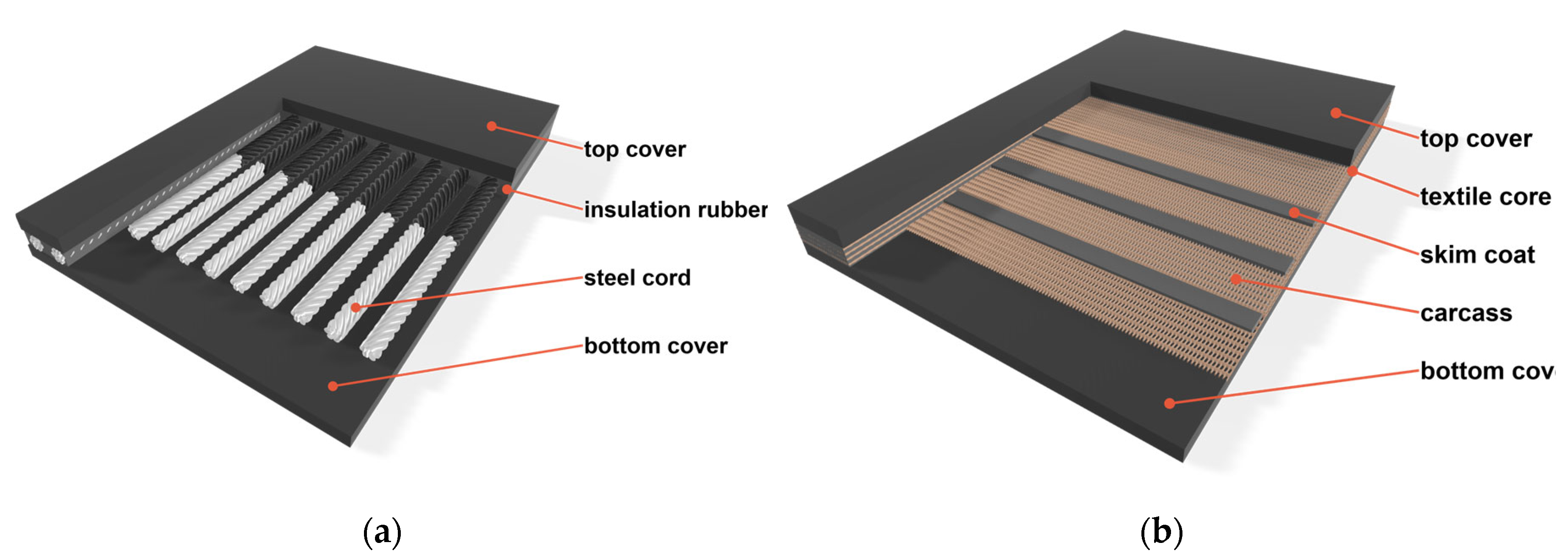
Figure 2.
Schematic of a closed-loop conveyor belt on a belt conveyor.
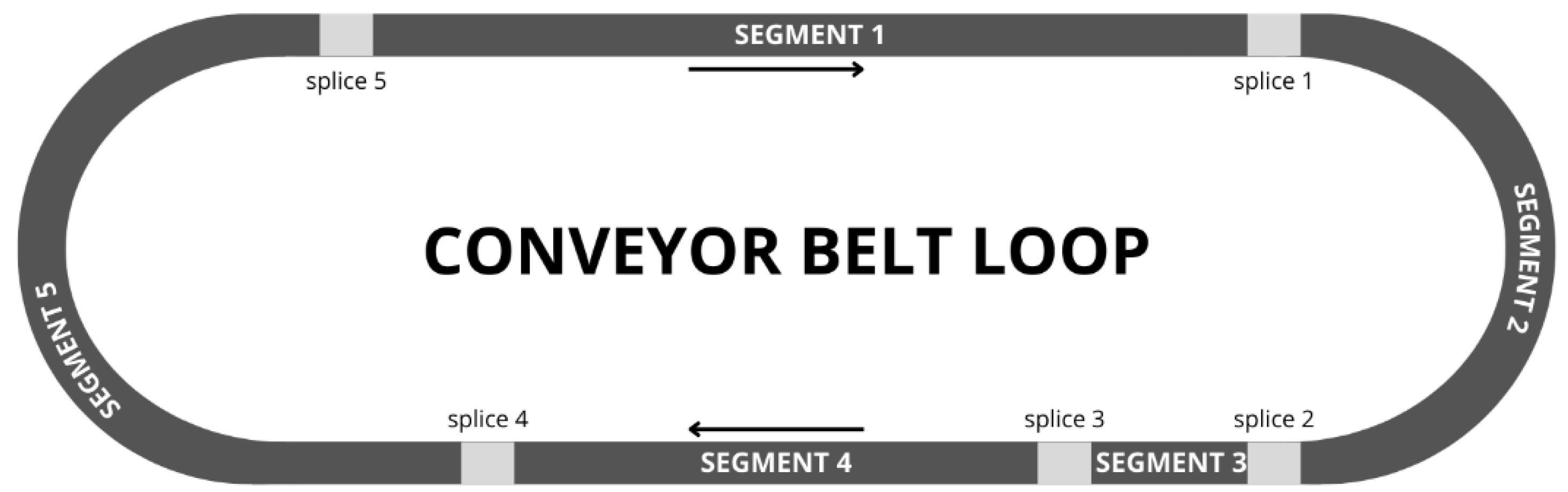
Figure 3.
Ishikawa diagram showing factors affecting splice durability and reliability.
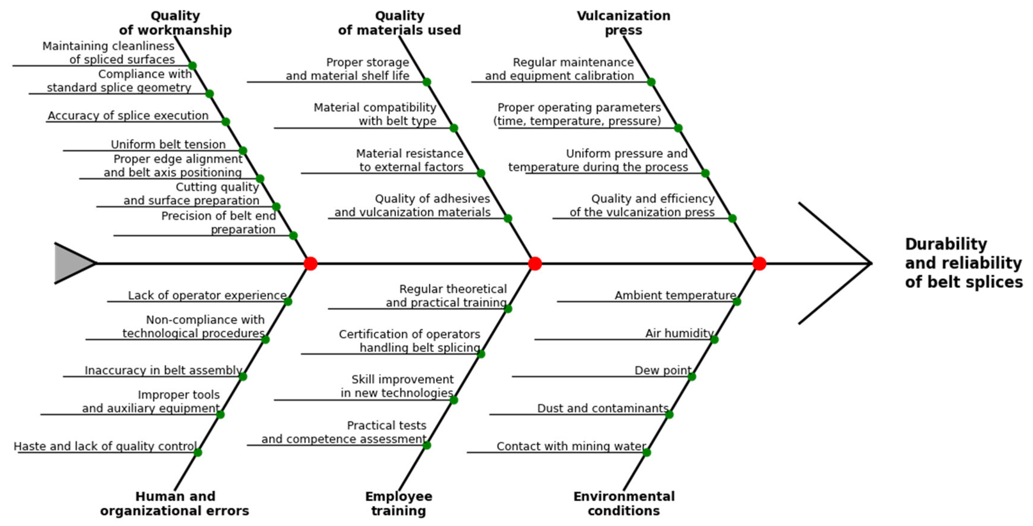
Figure 4.
Frame from an animation showing the installation of the measurement system on the conveyor (red-blue bars represent permanent magnet bars, the orange bar is the measurement head). A two-color signal image of splices and damage is shown on the belt.
Figure 4.
Frame from an animation showing the installation of the measurement system on the conveyor (red-blue bars represent permanent magnet bars, the orange bar is the measurement head). A two-color signal image of splices and damage is shown on the belt.
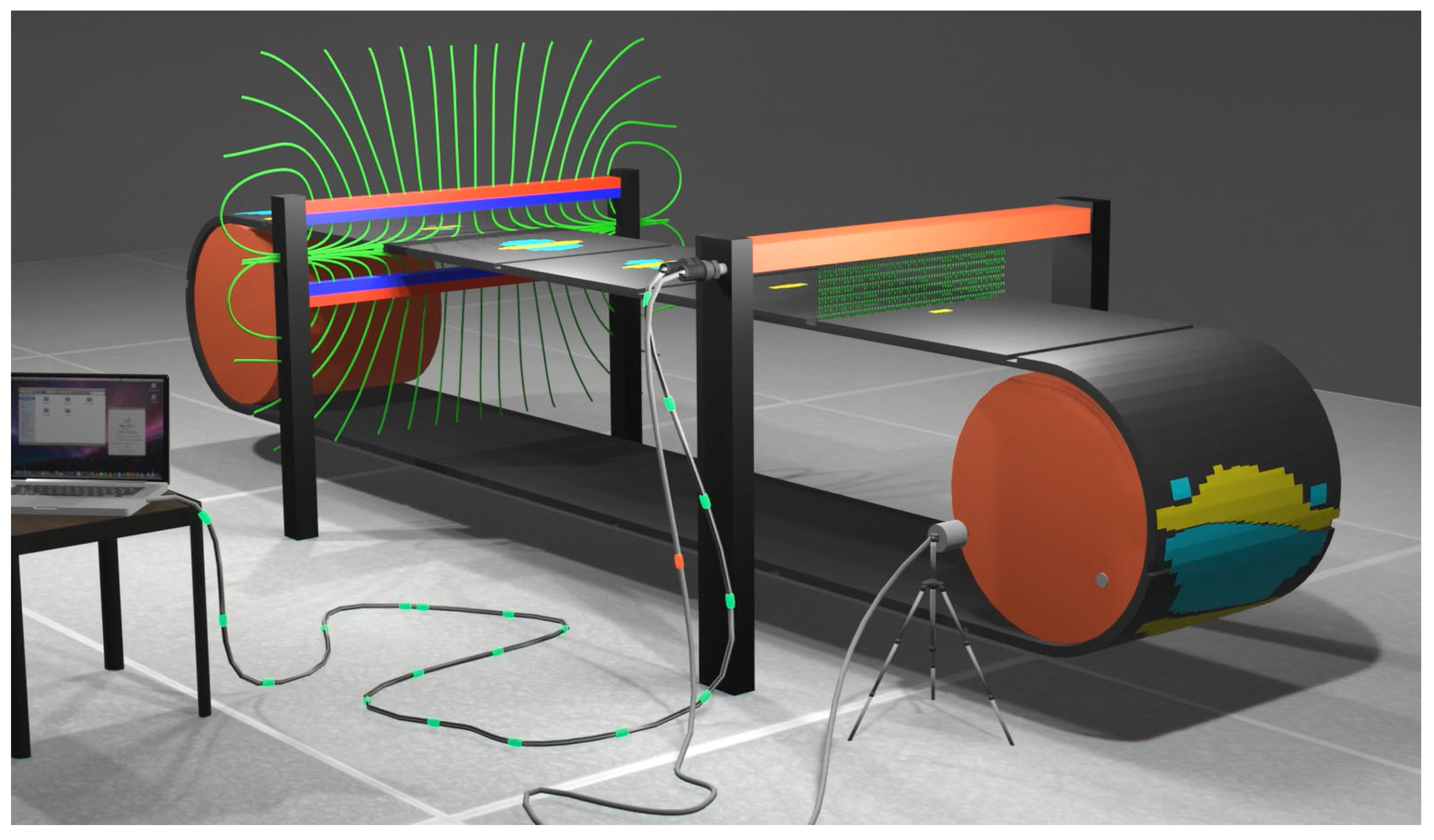
Figure 5.
Layout of the splices on the tested conveyor belt.
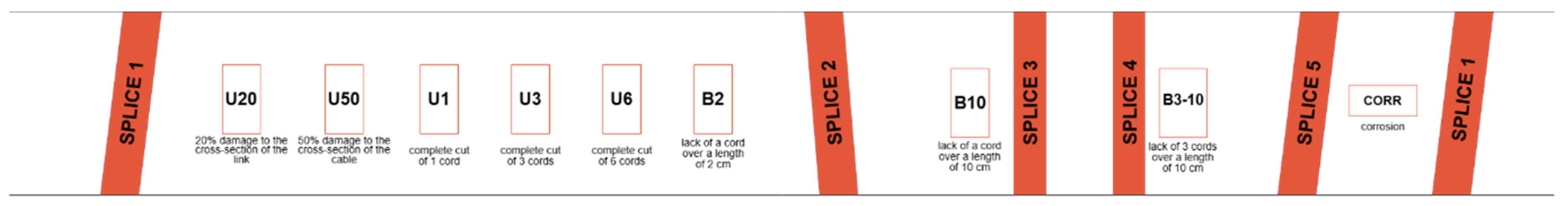
Figure 6.
Straight belt splice after milling the carrying cover, with measuring tape.
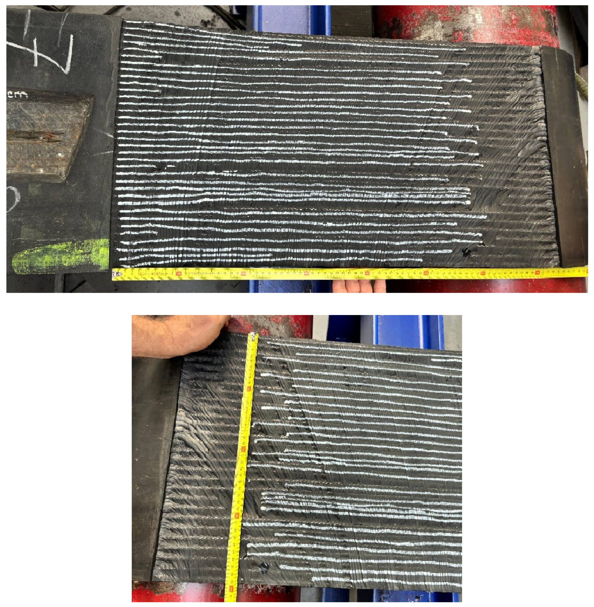
Figure 7.
Scarf belt splice after milling the carrying cover, with measuring tape.
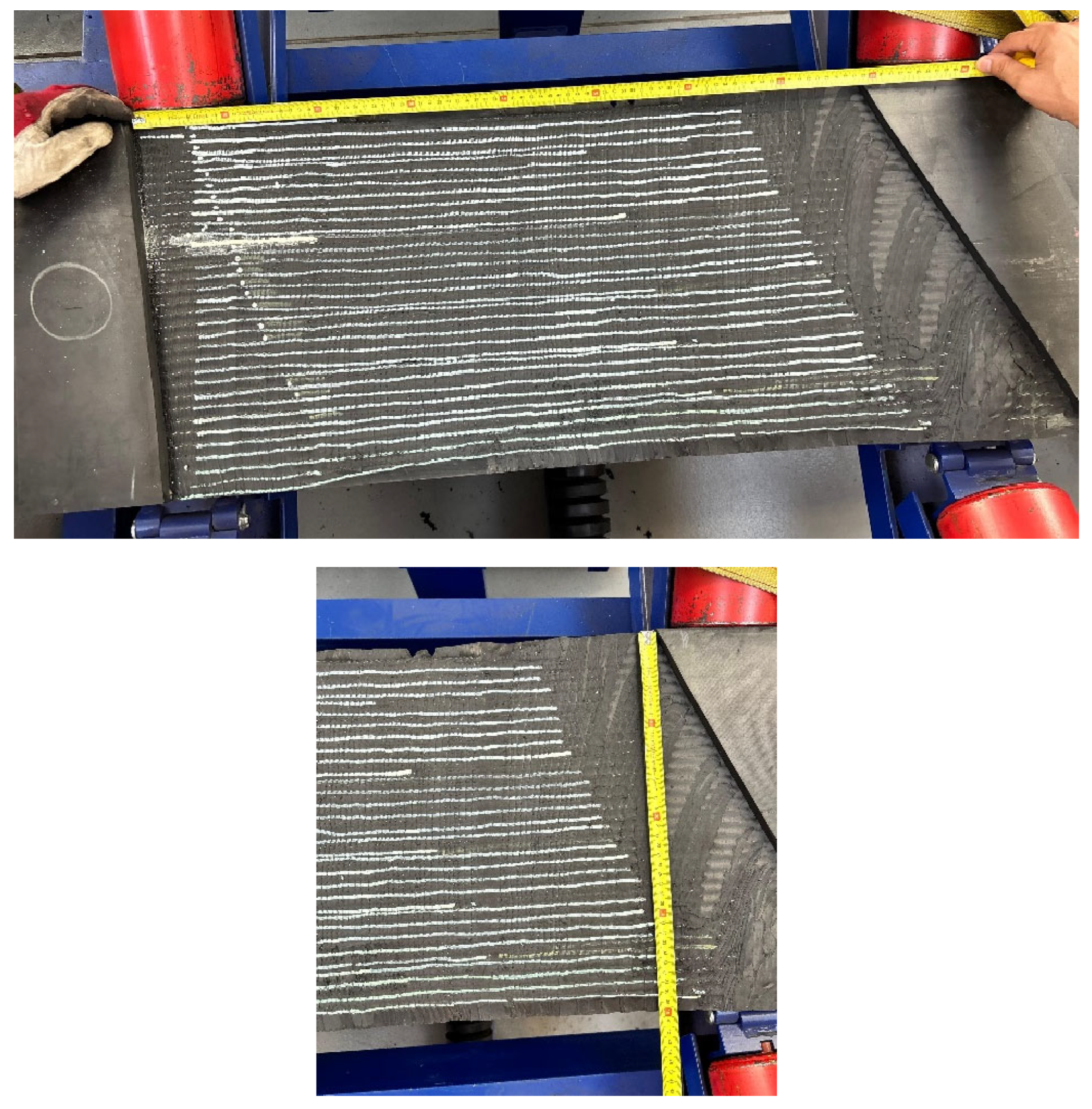
Figure 8.
DiagBelt+ measurement system installed on the conveyor belt in the Belt Transport Laboratory during measurements.
Figure 8.
DiagBelt+ measurement system installed on the conveyor belt in the Belt Transport Laboratory during measurements.
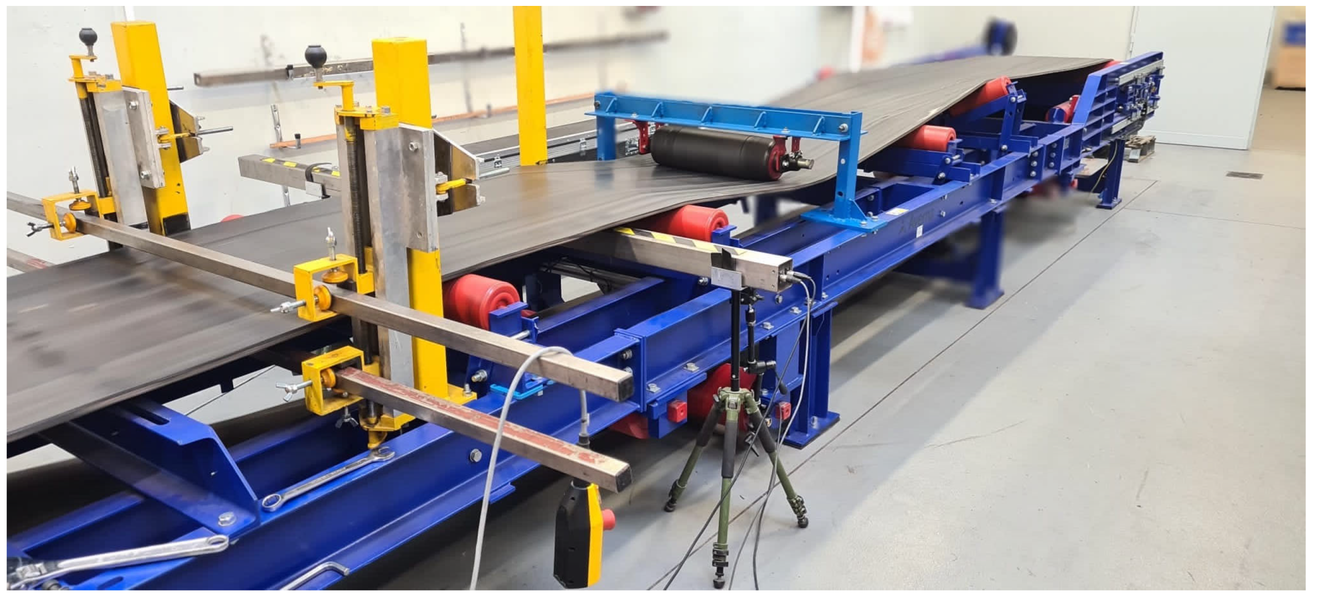
Figure 9.
Example of a measurement loop for different sets of measurement parameters.
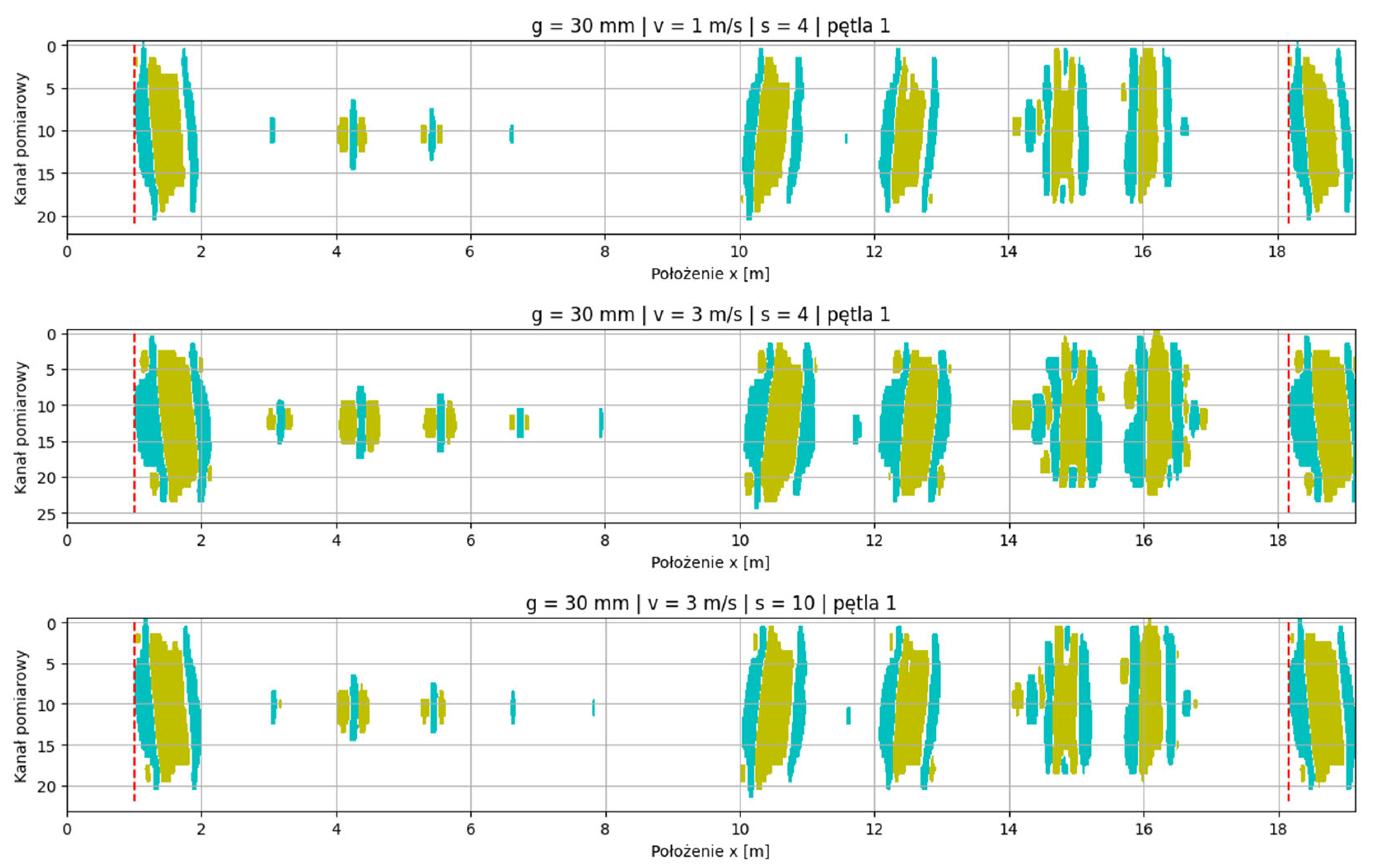
Figure 10.
Example of a magnetic signal of a conveyor belt splice.
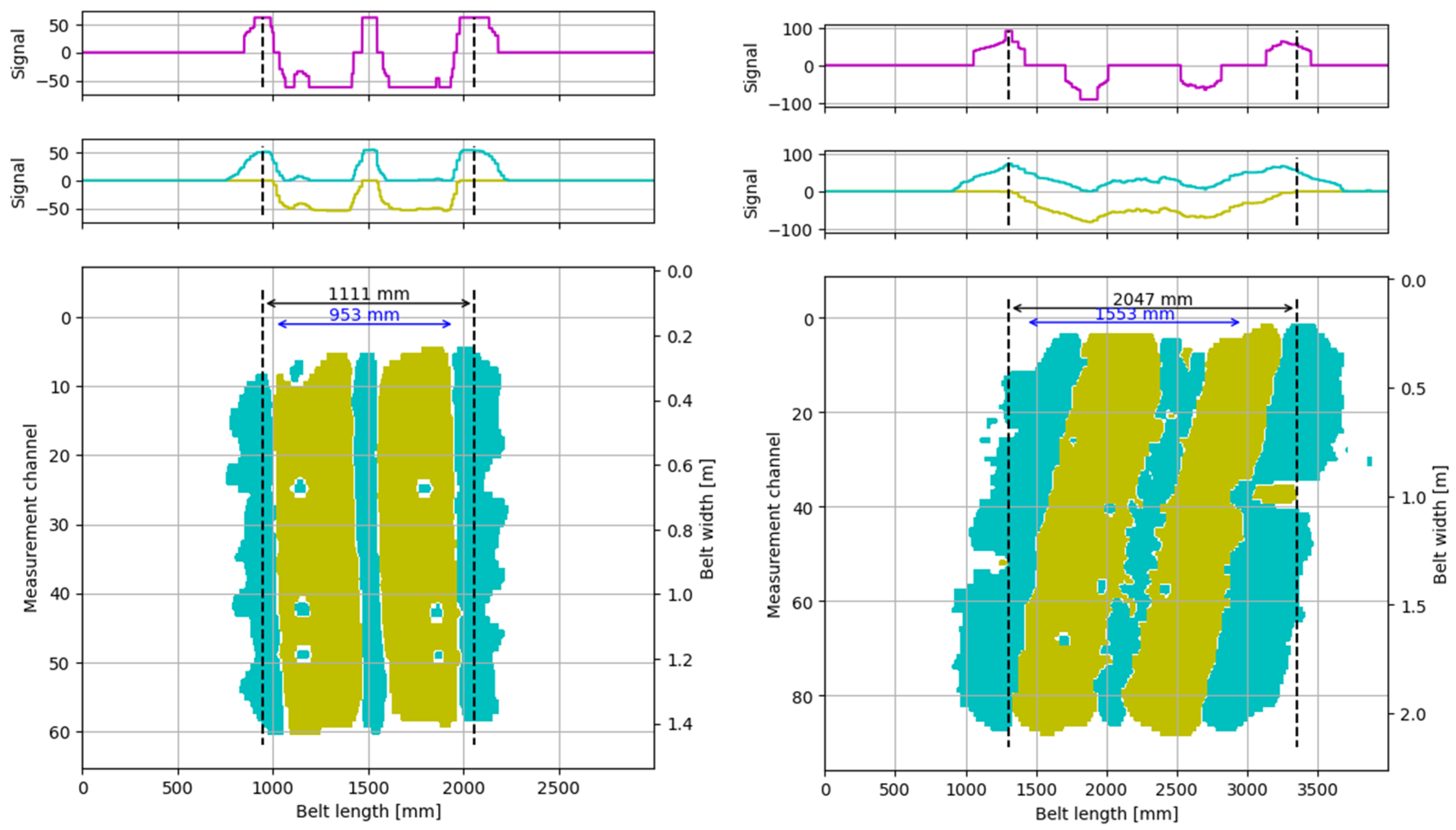
Figure 11.
Distribution of signal width (w-y-y) for splice no. 3 under different combinations of parameters g, v, and s.
Figure 11.
Distribution of signal width (w-y-y) for splice no. 3 under different combinations of parameters g, v, and s.
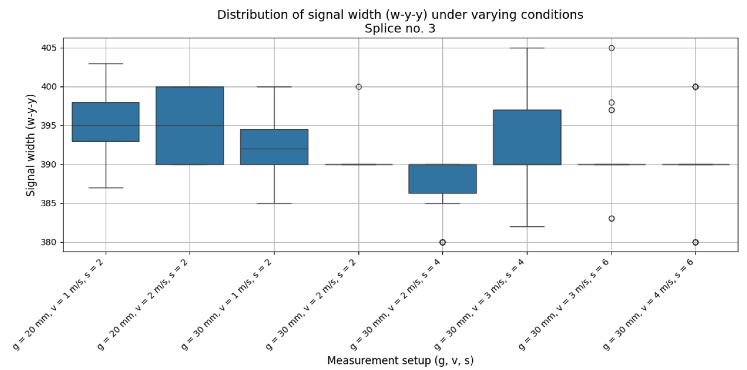
Figure 12.
Empirical distributions of the w-y-y signal width for individual splices.

Figure 13.
Empirical distributions of the w-y-y signal width for individual splices.
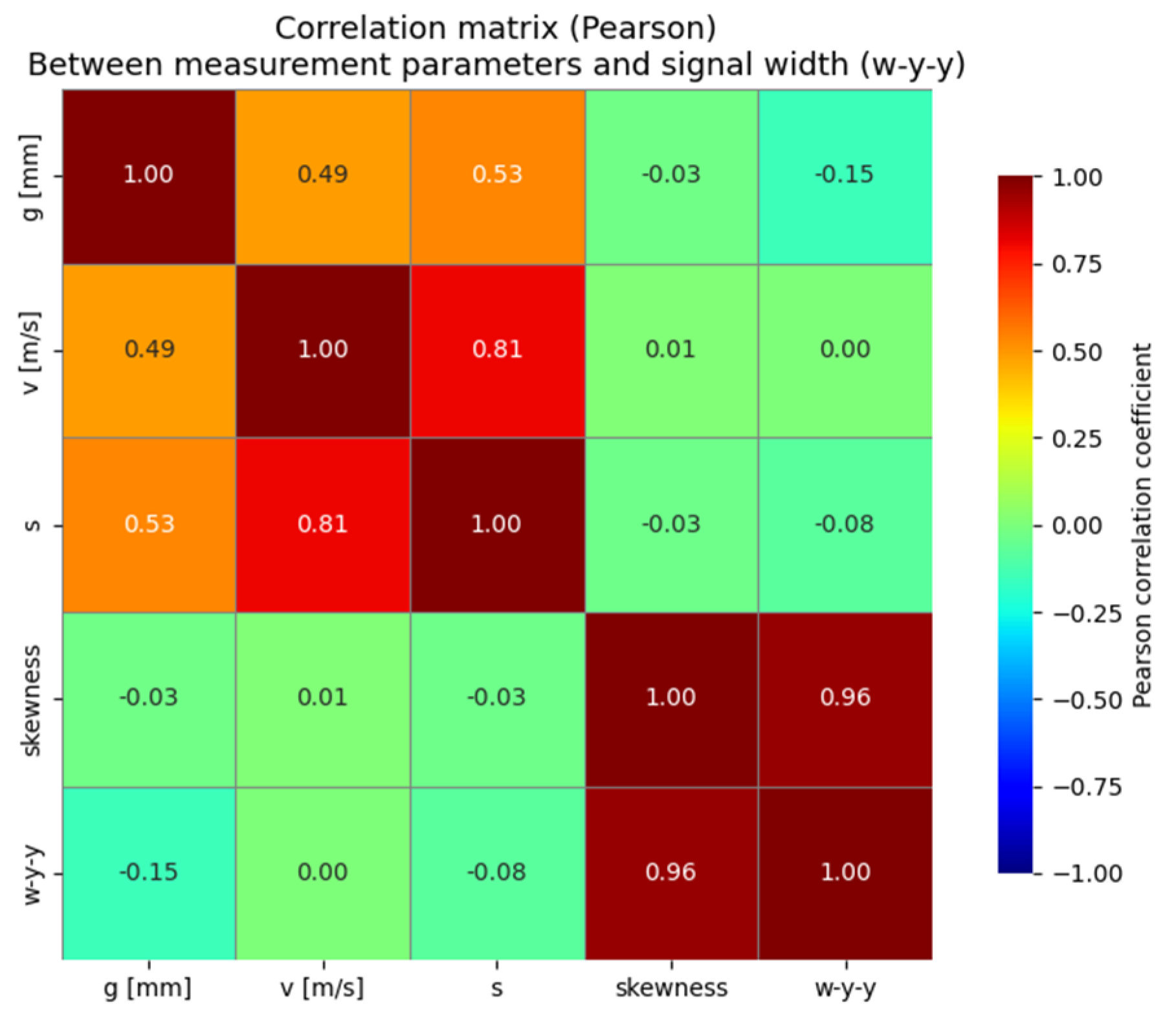

Table 1.
Descriptive statistics of the w-y-y variable for individual measurement configurations.
| splice | g [mm] | v [m/s] | s | N | mean | median | std | min | max | IQR |
| 1 | 20 | 1 | 2 | 45 | 497.98 | 497.0 | 3.12 | 492 | 505 | 5.0 |
| 1 | 20 | 2 | 2 | 50 | 530.20 | 530.0 | 9.79 | 490 | 550 | 0.0 |
| 1 | 30 | 1 | 2 | 45 | 478.71 | 478.0 | 3.53 | 472 | 490 | 5.0 |
| 1 | 30 | 2 | 2 | 49 | 489.49 | 490.0 | 4.59 | 480 | 500 | 0.0 |
| 1 | 30 | 2 | 4 | 50 | 490.70 | 490.0 | 3.03 | 485 | 500 | 0.0 |
| 1 | 30 | 3 | 4 | 50 | 487.36 | 487.5 | 5.81 | 472 | 503 | 1.0 |
| 1 | 30 | 3 | 6 | 50 | 494.00 | 495.0 | 4.58 | 487 | 510 | 0.0 |
| 1 | 30 | 4 | 4 | 50 | 488.20 | 490.0 | 6.29 | 470 | 500 | 7.5 |
| 1 | 30 | 4 | 6 | 50 | 486.20 | 490.0 | 4.90 | 480 | 490 | 10.0 |
| 2 | 20 | 1 | 2 | 50 | 488.54 | 490.0 | 10.89 | 460 | 502 | 8.0 |
| 2 | 20 | 2 | 2 | 20 | 489.75 | 490.0 | 8.50 | 480 | 505 | 16.3 |
| 2 | 30 | 1 | 2 | 50 | 441.96 | 443.0 | 11.65 | 415 | 467 | 16.5 |
| 2 | 30 | 2 | 2 | 30 | 469.33 | 470.0 | 7.04 | 455 | 480 | 3.8 |
| 2 | 30 | 2 | 4 | 50 | 464.40 | 460.0 | 8.67 | 430 | 480 | 10.0 |
| 2 | 30 | 3 | 4 | 43 | 477.09 | 473.0 | 9.70 | 458 | 495 | 14.5 |
| 2 | 30 | 3 | 6 | 50 | 471.72 | 472.0 | 6.97 | 465 | 495 | 8.0 |
| 2 | 30 | 4 | 4 | 4 | 480.00 | 480.0 | 8.16 | 470 | 490 | 5.0 |
| 2 | 30 | 4 | 6 | 40 | 477.00 | 480.0 | 9.92 | 460 | 490 | 12.5 |
| 3 | 20 | 1 | 2 | 50 | 395.26 | 395.0 | 3.32 | 387 | 403 | 5.0 |
| 3 | 20 | 2 | 2 | 4 | 395.00 | 395.0 | 5.77 | 390 | 400 | 10.0 |
| 3 | 30 | 1 | 2 | 50 | 392.18 | 392.0 | 3.57 | 385 | 400 | 4.5 |
| 3 | 30 | 2 | 2 | 9 | 391.11 | 390.0 | 3.33 | 390 | 400 | 0.0 |
| 3 | 30 | 2 | 4 | 50 | 387.80 | 390.0 | 3.93 | 380 | 390 | 3.8 |
| 3 | 30 | 3 | 4 | 49 | 392.73 | 390.0 | 4.54 | 382 | 405 | 7.0 |
| 3 | 30 | 3 | 6 | 50 | 390.46 | 390.0 | 3.11 | 383 | 405 | 0.0 |
| 3 | 30 | 4 | 6 | 50 | 390.20 | 390.0 | 4.73 | 380 | 400 | 0.0 |
| 4 | 20 | 1 | 2 | 50 | 385.76 | 385.0 | 3.86 | 377 | 393 | 4.5 |
| 4 | 20 | 2 | 2 | 50 | 397.80 | 400.0 | 4.30 | 390 | 405 | 0.0 |
| 4 | 30 | 1 | 2 | 50 | 381.94 | 382.0 | 3.91 | 375 | 392 | 6.5 |
| 4 | 30 | 2 | 2 | 50 | 389.10 | 390.0 | 4.25 | 380 | 400 | 0.0 |
| 4 | 30 | 2 | 4 | 46 | 382.61 | 380.0 | 4.91 | 370 | 390 | 10.0 |
| 4 | 30 | 3 | 4 | 50 | 381.68 | 382.0 | 4.65 | 367 | 390 | 1.0 |
| 4 | 30 | 3 | 6 | 50 | 379.76 | 382.0 | 4.25 | 367 | 390 | 8.0 |
| 4 | 30 | 4 | 4 | 50 | 383.00 | 380.0 | 5.44 | 370 | 400 | 10.0 |
| 4 | 30 | 4 | 6 | 50 | 381.20 | 380.0 | 5.21 | 370 | 400 | 0.0 |
| 5 | 20 | 1 | 2 | 49 | 508.29 | 508.0 | 7.06 | 495 | 523 | 12.0 |
| 5 | 20 | 2 | 2 | 50 | 504.70 | 500.0 | 5.66 | 500 | 520 | 10.0 |
| 5 | 30 | 1 | 2 | 36 | 496.00 | 496.0 | 8.14 | 482 | 515 | 8.0 |
| 5 | 30 | 2 | 2 | 50 | 496.10 | 500.0 | 6.95 | 480 | 510 | 10.0 |
| 5 | 30 | 2 | 4 | 17 | 487.35 | 490.0 | 5.34 | 480 | 500 | 5.0 |
| 5 | 30 | 3 | 4 | 50 | 499.34 | 502.0 | 6.96 | 480 | 517 | 8.0 |
| 5 | 30 | 3 | 6 | 43 | 492.88 | 495.0 | 6.46 | 480 | 510 | 7.5 |
| 5 | 30 | 4 | 4 | 50 | 489.60 | 490.0 | 4.50 | 480 | 500 | 0.0 |
| 5 | 30 | 4 | 6 | 50 | 494.40 | 490.0 | 5.41 | 490 | 510 | 10.0 |
Disclaimer/Publisher’s Note: The statements, opinions and data contained in all publications are solely those of the individual author(s) and contributor(s) and not of MDPI and/or the editor(s). MDPI and/or the editor(s) disclaim responsibility for any injury to people or property resulting from any ideas, methods, instructions or products referred to in the content. |
© 2025 by the authors. Licensee MDPI, Basel, Switzerland. This article is an open access article distributed under the terms and conditions of the Creative Commons Attribution (CC BY) license (http://creativecommons.org/licenses/by/4.0/).
Copyright: This open access article is published under a Creative Commons CC BY 4.0 license, which permit the free download, distribution, and reuse, provided that the author and preprint are cited in any reuse.


