Submitted:
08 April 2025
Posted:
08 April 2025
You are already at the latest version
Abstract
The characteristics of aeroengine components at sub-idle conditions are difficult to obtain directly through experiments and must be extrapolated from the characteristics above idle. However, existing extrapolation methods face issues such as incomplete utilization of available data, infeasibility under limited available data, and inability to completely cap-ture the unique operating modes of the components. To address these challenges, this pa-per proposes an extrapolation method for sub-idle component characteristics of aeroen-gines based on curve and surface fitting. In consideration of the smooth and continuous nature of engine component characteristics, the method performs curve and surface fitting on the above-idle characteristics and extrapolates sub-idle characteristics from the fitting results. The method is applied to extrapolate the compressor and turbine characteristics of a micro turbojet engine and validate the results through ground-start simulations under different inlet conditions. The results demonstrate that the method effectively overcomes the limitations of existing extrapolation methods and meets the requirements for simulat-ing the ground start process of aeroengines under various inlet conditions.
Keywords:
Aeroengine
; Component Characteristic
; Extrapolation
; Curve
; Surface
; Fitting
1. Introduction
Component-level mathematical models for aero-engines are vital tools for the development of engine control systems, where component characteristics form the foundation for modeling. Characteristics above idle can be obtained through bench tests or directly by using modified generic characteristics when bench test is unavailable. However, acquiring sub-idle characteristics through similar methods is challenging [1]. Hence, it is necessary to extrapolate sub-idle characteristics based on above-idle data to meet the requirements for start-up process simulations.
Researchers often face the limitation of insufficient data to support the extrapolation [2]. This requires the extrapolation method to be applicable with limited available data and to make full use of it. Furthermore, during the start-up process of an aeroengine, components enter unique operating modes [3]: compressors may operate in stirring or turbine modes, and turbines may function in stirring or compressor modes. Ensuring reasonable and complete reflection of these unique modes is crucial in component characteristic extrapolation.
Based on findings from the literature, the extrapolation of aero-engine component characteristics is commonly performed using the following methods:
1. Proportional Coefficient Method
Proposed by Agrawal and Yunis, this approach extrapolates sub-idle component characteristics using similarity principles, establishing proportional relationships between corrected flow, pressure ratio, specific work, and corrected speed based on known above-idle performance [4]. Sexton later extended its application to turbine characteristics, making it analogous to compressors [5]. Gaudet and Gauthier [6], along with Zhou Wenxiang [7], refined the method’s equations to suit various engine components. While computationally straightforward, it relies solely on one or two known speed lines and fails to reflect unique operating modes.
Researchers have introduced modifications: Rao Gao et al. incorporated Support Vector Machines (SVM) to enhance accuracy, though the method’s inability to capture unique operating modes persisted [8]. Hao Wang et al. replaced isentropic efficiency with corrected torque, achieving better representation of component-specific operating modes but leaving the issue of underutilized data unresolved [9,10].
2. Stage Stacking Method
Developed by NASA [11], this technique derives full compressor characteristics by stacking known single-stage axial compressor data. It has been applied by Yan [12], Ju Xinxing [13], and NASA Lewis Research Center [14] to extrapolate sub-idle characteristics for axial, combined, and fan compressors. Despite its adaptability to various compressors, the method requires detailed design parameters and is not suitable for turbines.
3. Zero-Speed Line Interpolation Method
This approach interpolates sub-idle characteristics using above-idle data and zero-speed characteristics, which are obtained through experiments or CFD. Applications by Zachos [15,16] and Jialin Zheng [17] have demonstrated its effectiveness. However, its reliance on precise zero-speed characteristics makes implementation challenging [18].
4. Backbone Feature Method
Developed collaboratively by General Electric and NASA Lewis Research Center [19,20,21], this method extrapolates component characteristics by parameterizing backbone and non-backbone point data and analyzing their trends across the speed range. With the help of it, Shi Yang established full-state models for a civilian high-bypass turbofan engine [3] and a single-rotor turbojet engine [22]; Wang Jiamei [23] achieved windmilling state simulations for a military turbofan engine, and Fang Yun [24] performed ground start and high-altitude windmilling start simulations for a turbofan engine. Although capable of capturing unique operating modes, it cannot extrapolate to zero speed.
5. β Extrapolation Method
This method was proposed by Dr. Kurzke, the author of the engine performance simulation software GasTurb, and is incorporated into the compressor and turbine characteristic processing software SmoothC and SmoothT [25,26]. Kurzke conducted a detailed analysis of characteristic maps and CFD simulation results for a variety of compressors, and based on this, summarized the relationships between physical quantities such as corrected flow, specific work, torque, and exit guide vane throat Mach number at low speeds [27]. He introduced an intermediate variable, , which will be elaborated in the following sections, and reasonably estimated the zero-speed characteristics of the compressor, ultimately forming the extrapolation method [28]. This method has been extended to turbines [29], and its extrapolated results have been successfully applied in ground and windmilling start simulations [30]. Additionally, Kurzke modified the definition of the line at low speeds to ensure that the extrapolated results meet simulation requirements at 1% of the design speed [31]. The method has a solid theoretical foundation, a rigorous logical process, and scientifically reasonable extrapolated results, but requires supporting software for implementation.
In summary, existing extrapolation methods struggle to fully utilize limited available data and accurately reflect the unique operating modes of components. To tackle this issue, this study proposes a curve- and surface-fitting-based extrapolation method for sub-idle characteristics of aeroengine components. Section 2, Methodology, introduces the general expression of component characteristics and presents above-idle characteristics of a micro turbojet engine as known data. It then analyzes the full-state operating features of compressors and turbines, identifying key issues for achieving comprehensive extrapolation, and concludes with a detailed description of the method’s implementation. Section 3, Results and Simulation Verification, presents the extrapolated characteristics, outlines simulation preparations, and demonstrates ground start simulations under varying inlet conditions. Section 4, Conclusion, summarizes that the proposed method overcomes limitations of existing approaches, comprehensively utilizes limited data, accurately captures unique operating modes, and meets the simulation requirements for aeroengine ground starts under different conditions.
2. Methodology
2.1. General Expression of Aircraft Engine Component Characteristics
In aircraft engine component-level model, component characteristics such as corrected flow, compressor pressure ratio, turbine pressure ratio, and isentropic efficiency are often represented as a 2D array, with the relative corrected speed as the row parameter and intermediate variables as the column parameter. In component characteristic maps, the component characteristics are presented in the form of relative corrected speed lines. Compressor characteristics are plotted on two graphs, with the horizontal axis representing corrected flow and the vertical axis representing pressure ratio and isentropic efficiency, respectively. Similarly, for two turbine characteristic maps, the horizontal axis represents the product of corrected flow and relative corrected speed [32], and the vertical axis represents pressure ratio and isentropic efficiency, respectively.
The primary role of the intermediate variables is to determine the engine operating point’s location on the characteristic map. Two commonly used intermediate variables are the pressure ratio coefficient and . The former includes the compressor pressure ratio coefficient and the turbine pressure ratio coefficient, defined by Equations (1) and (2), respectively.
In the equations, is the pressure ratio coefficient, is the pressure ratio, and the subscripts and represent the compressor and turbine, respectively. The subscripts max and min represent the maximum and minimum values at the same relative corrected speed. From equations (1) and (2), it can be concluded that the range of values for the pressure ratio coefficient is .
If the compressor pressure ratio and turbine pressure ratio monotonically vary with corrected flow across all relative corrected speed lines, the pressure ratio coefficient can be used as the intermediate variable. Otherwise, should be used as the intermediate variable [31]. The curves are a set of equidistant parabolas on characteristic maps where the vertical axis represents pressure ratio. These parabolas are parameterized by the intermediate variable , and their intersections with the relative corrected speed lines define the component characteristic points. The values of for the top and bottom parabolas are 1 and 0, respectively, so the range of is also .
The design-point inlet conditions for the micro turbojet engine in this study are standard atmospheric conditions at sea level, with an inlet Mach number of 0. The design-point parameters are listed in Table 1.
The rotating components of the engine consist of a single-stage centrifugal compressor and a single-stage axial turbine. Based on ground test data from the micro turbojet engine, the generic component characteristics were corrected to obtain the above-idle characteristics of the compressor and turbine, as shown in Figure 1 and Figure 2.
Figure 1.
Compressor characteristic maps above idle.
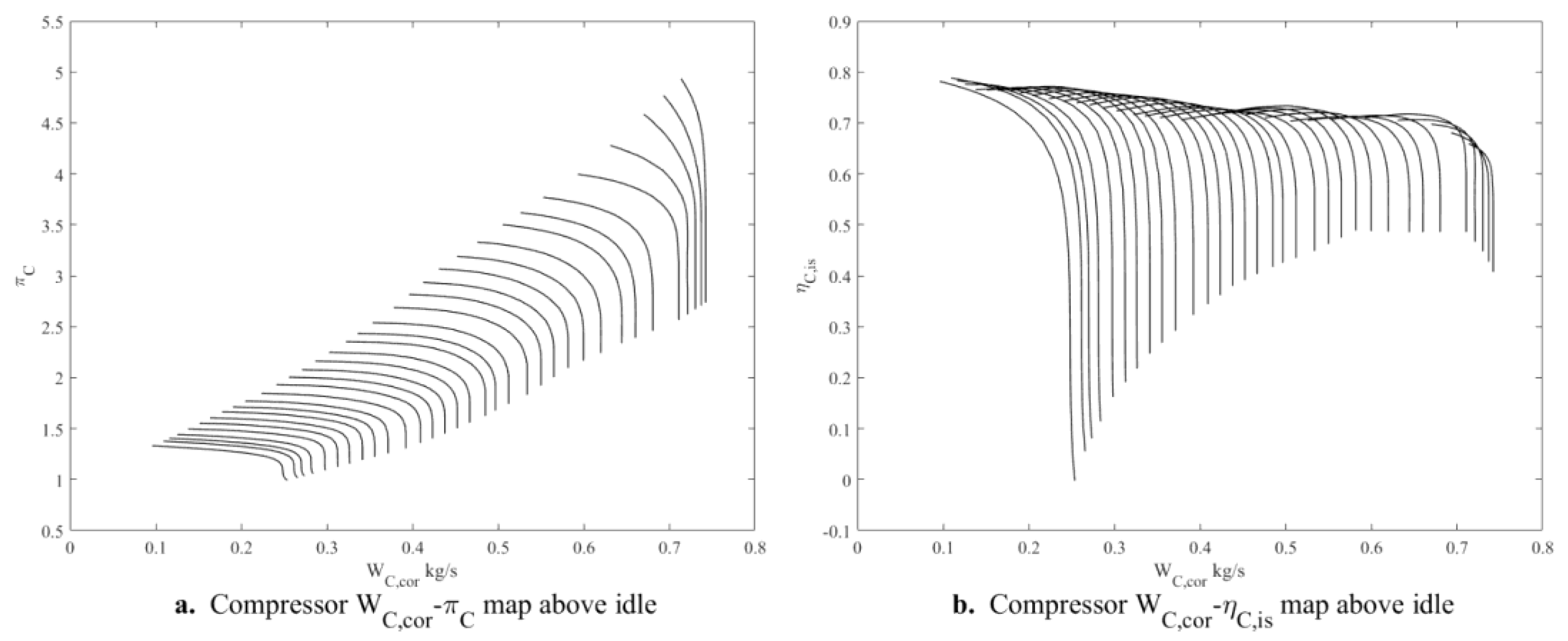
Figure 2.
Turbine characteristic maps above idle.
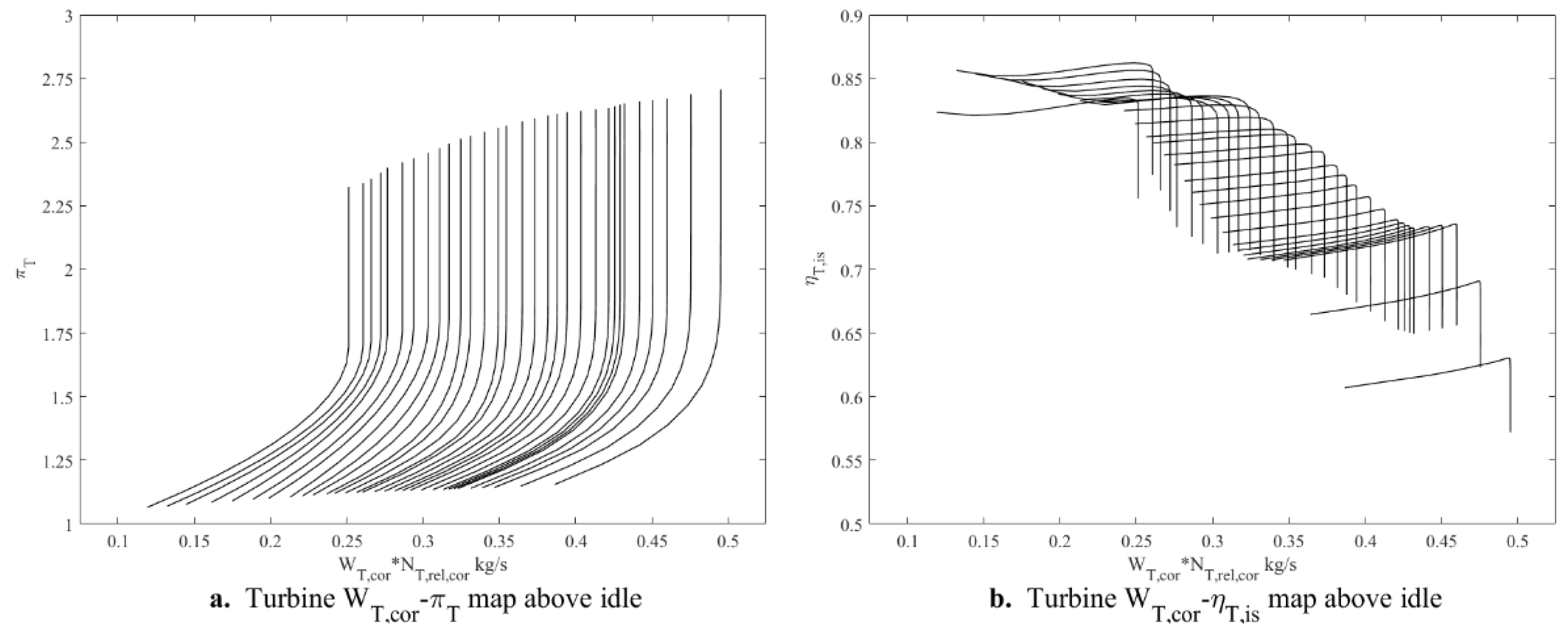
In Figure 1 and Figure 2 above, the relative corrected speeds corresponding to the relative corrected speed lines increase gradually from left to right. For the compressor, the minimum relative corrected speed is 0.4, and the maximum is 1.12; for the turbine, the minimum relative corrected speed is 0.55, and the maximum is 1.1. Since the compressor pressure ratio and turbine pressure ratio vary monotonically with corrected flow across all relative corrected speed lines, the pressure ratio coefficient is used as the intermediate variable. Apart from the above-idle component characteristics, other data, including geometric parameters, are unavailable, meaning that the extrapolation of component characteristics must rely solely on the limited available data.
2.2. Analysis of the Operating Modes of Aeroengine Compressors and Turbines
During the operation of an aircraft engine, the compressor may operate in the following three modes [3]:
(1) Compressor Mode
This is the standard operating mode, where the compressor consumes power to compress the airflow. In this mode, the following condition applies:
In the equations:
represents temperature, measured in Pa;
represents temperature, measured in K;
represents enthalpy, measured in J;
represents specific enthalpy change, it has the same unit with ;
represents the isentropic efficiency of the compressor.
The subscripts:
denote total parameters,
denote the isentropic process,
and denote the component inlet and outlet, respectively.
(2) Stirring Mode
At low rotational speeds, the compressor may enter a unique mode where the work done on the airflow is insufficient to overcome flow losses. Thus, the following condition applies:
(3). Turbine Mode
When the compressor is in a windmilling condition, it may behave like a turbine, with airflow performing work on it and causing rotation. Under these circumstances, the following conditions exist:
In contrast, the turbine may operate in the following three modes:
1. Turbine Mode
This normal mode involves airflow expanding within the turbine and performing work on it. The conditions are as follows:
2. Stirring Mode
During ground startup, the turbine may enter a stirring mode, where similar conditions to the compressor’s stirring mode exist:
3. Compressor Mode
In a windmilling start, the turbine behaves like a compressor, consuming power to compress the airflow. The following conditions are applicable:
The micro turbojet engine discussed in this study has no compressor bleed air and no turbine cooling air; therefore, the following conditions apply:
In the equation, is the gas mass flow rate, measured in kg/s.
Thus, the isentropic efficiencies of the compressor and turbine can be calculated using Equations (35) and (36), respectively:
where, represents the specific enthalpy of the gas, which is the enthalpy per unit mass of the gas, and is the change in specific enthalpy, both of them are measured with J/kg.
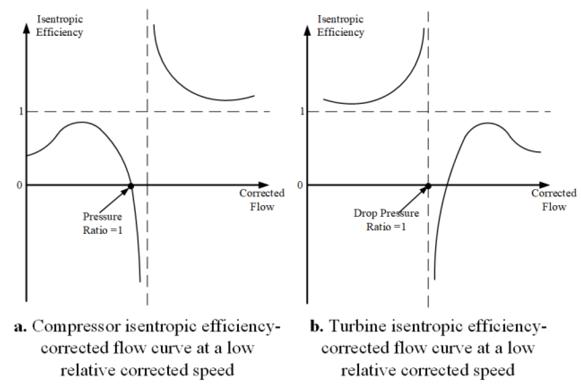
When the relative corrected speed is low, considering the relative corrected speed is kept constant, the isentropic efficiencies of the compressor and turbine vary with the corrected flow rate, as shown in Figure 3. It can be seen that the isentropic efficiency is discontinuous. Therefore, to make the extrapolation results reasonable and adequately reflect the unique operating modes of the components, it is necessary to overcome the impact of the discontinuity in isentropic efficiency.
Figure 2.
Isentropic efficiency-corrected flow curves at a low relative corrected speed.
2.3. Extrapolation Method for Component Characteristics Below Idle Based on Curve and Surface Fitting
Based on the continuous and smooth nature of aircraft engine component characteristics [32], a method is proposed for extrapolating component characteristics below idle using curve and surface fitting. This method fully utilizes the limited available data to extrapolate component characteristics and ensures that the extrapolation results are reasonable and adequately reflect the unique operating modes of the components. The method includes extrapolation techniques for both the compressor and turbine characteristics. The micro turbojet engine in this study is used as the application object for the method, and the extrapolation steps are carried out using the Curve Fitting tool in MATLAB R2023b.
2.3.1. Compressor Component Characteristics Extrapolation Method
To extrapolate the compressor component characteristics, the following steps should be followed:
Step 1: Fit the curves of the maximum and minimum pressure ratios above idle as a function of the relative corrected speed. The fitting relationships are given by Equations (37) and (38), and the maximum and minimum pressure ratios below idle are extrapolated from the fitting results.
In the formula, represents the curve, and is the compressor’s relative corrected speed, defined as follows:
In the formula, represents the mechanical speed, and is the sea-level static temperature under standard atmospheric conditions.
Considering that when the speed is 0, the compressor cannot perform work on the airflow, the fitting process should incorporate the following constraints: For the maximum pressure ratio, a constraint should be applied such that the maximum pressure ratio equals 1 when the relative corrected speed is 0. For the minimum pressure ratio, a specific value should be specified within the range as the constraint when the relative corrected speed is 0.
For the micro turbojet engine, a Piecewise Cubic Hermite Polynomial Interpolation method (PCHPI) is used to fit the curves of the maximum and minimum pressure ratios above idle. Additionally, it is specified that the minimum pressure ratio is 0.75 when the relative corrected speed is 0. The fitting and extrapolation results are shown in Figure 4.
Step 2: Based on the extrapolated results of the maximum and minimum pressure ratios, the pressure ratios at other points below idle are calculated using Equation (40).
Step 3: Fit the curves of the maximum and minimum corrected flow rates above idle as a function of the relative corrected speed. The fitting relationships are given by Equations (41) and (42), and the maximum and minimum corrected flow rates below idle are extrapolated from the fitting results.
In the equation, represents the compressor corrected flow rate, which is defined as follows:
Considering that when the speed is 0, if the pressure ratio is 1, there is no pressure difference between the inlet and outlet, and the flow rate should be 0; if the pressure ratio is less than 1, the total pressure at the inlet is greater than that at the outlet, and the flow rate should be greater than 0. Therefore, during fitting, for the minimum corrected flow rate, a constraint should be applied such that the minimum corrected flow rate equals 0 when the relative corrected speed is 0. For the maximum corrected flow rate, a value greater than 0 should be specified as the constraint when the relative corrected speed is 0.
Regarding the micro turbojet engine, PCHPI is used to fit the curves of the maximum and minimum corrected flow rates above idle, and it is specified that the maximum corrected flow rate equals 0.1 kg/s when the relative corrected speed is 0. The fitting and extrapolation results are shown in Figure 5a.
Step 4: Based on the corrected flow rates above idle and the maximum and minimum corrected flow rates below idle, perform a surface fitting of the corrected flow rate as a function of the relative corrected speed and pressure ratio coefficient. The fitting relationship is given by Equation (44), and the corrected flow rates at other points below idle are extrapolated from the fitting results.
In the equation, represents the surface.
Concerning the micro turbojet engine, a thin-plate spline method is used to perform surface fitting of the corrected flow rate. The fitting and extrapolation results are shown in Figure 5b.
Step 5: To address the issue of discontinuity in isentropic efficiency, the extrapolation of isentropic efficiency should be converted into the extrapolation of corrected specific enthalpy change. However, the corrected specific enthalpy change above idle is unknown. Therefore, the compressor specific enthalpy change coefficient is defined as follows:
In the equation, represents the compressor specific enthalpy change coefficient, is the approximate value of the average specific heat ratio of the gas in the compressor, and in this study, .
For the compressor, at any relative corrected speed, if , then , and is continuously differentiable at this point. According to L’Hôpital’s rule, exists and is a constant. Thus, it can be concluded that is continuous.
The compressor corrected specific enthalpy change can be calculated using the following equation:
In the equation, represents the compressor corrected specific enthalpy change, while and are the average specific heat capacity at constant pressure and the average specific heat ratio of the gas in the compressor, respectively. From Equations (45) and (46), it can be concluded that is positively correlated with .
In summary, converting the extrapolation of isentropic efficiency into the extrapolation of the specific enthalpy change coefficient resolves the issues of isentropic efficiency discontinuity and the unknown corrected specific enthalpy change above idle. From Equation (45), Equation (47) can be derived. Using Equation (47), the corresponding isentropic efficiency can be calculated from the extrapolated results of the specific enthalpy change coefficient, thereby indirectly achieving the extrapolation of isentropic efficiency.
With the help of Equation (45), we can calculate the specific enthalpy change coefficients for each point above idle. Perform curve fitting of the specific enthalpy change coefficients corresponding to the maximum and minimum pressure ratios above idle as functions of the relative corrected speed. The fitting relationships are given by Equations (48) and (49), and the specific enthalpy change coefficients corresponding to the maximum and minimum pressure ratios below idle are extrapolated from the fitting results.
When the speed is 0, if the pressure ratio equals 1, the flow rate is 0, and there is no energy exchange between the compressor and the airflow. Consequently, the specific enthalpy change coefficient should theoretically be 0. However, for the specific enthalpy change coefficient corresponding to the maximum pressure ratio, a value greater than 0 must still be specified as a constraint when the relative corrected speed is 0. This is because the compressor at zero speed can only operate in the stirring mode or turbine mode. As the pressure ratio gradually decreases from 1, the stirring mode should appear first, followed by the turbine mode. Correspondingly, the isentropic efficiency should first decrease from 0 to , and then continue to decrease from .From Equation (47), it can be deduced that only when the specific enthalpy change coefficient at zero speed starts from a value greater than 0 and decreases with the pressure ratio until it becomes less than 0, the isentropic efficiency at zero speed can exhibit such a variation.
When the speed is 0 and the pressure ratio is less than 1, the flow rate is greater than 0. The airflow loses energy as it passes through the compressor, and the specific enthalpy change coefficient should be less than 0. Therefore, during fitting, for the specific enthalpy change coefficient corresponding to the minimum pressure ratio, a value less than 0 should be specified as a constraint when the relative corrected speed is 0. After extrapolation, if the isentropic efficiency is found to be less than 1 when the pressure ratio is less than 1, the constraint conditions should be adjusted, and the extrapolation process should be repeated.
In the case of the micro turbojet engine, the specific enthalpy change coefficients corresponding to the maximum and minimum pressure ratios above idle are fitted using a 4th-order Gaussian fitting method and PCHPI, respectively. It is specified that the specific enthalpy change coefficient corresponding to the minimum pressure ratio is -0.04 when the relative corrected speed is 0. Without applying constraints to the specific enthalpy change coefficient corresponding to the maximum pressure ratio, the extrapolation results do not violate the principle that this coefficient must be greater than 0 at a relative corrected speed of 0. The fitting and extrapolation results are shown in Figure 6a.
Step 6: Based on the specific enthalpy change coefficients above idle and those corresponding to the maximum and minimum pressure ratios below idle, perform surface fitting of the specific enthalpy change coefficient as a function of the relative corrected speed and pressure ratio coefficient. The fitting relationship is given by Equation (50), and the specific enthalpy change coefficients at other points below idle are extrapolated from the fitting results.
As pertains to the micro turbojet engine, a thin-plate spline method is used to perform surface fitting of the specific enthalpy change coefficients. The fitting and extrapolation results are shown in Figure 6b.
2.3.2. Turbine Component Characteristics Extrapolation Method
For the turbine component characteristics extrapolation, the following procedure applies:
Step 1: Perform curve fitting for the maximum and minimum turbine pressure ratios above idle as functions of the relative corrected speed. The fitting relationships are given by Equations (51) and (52). The maximum and minimum turbine pressure ratios below idle are extrapolated based on the fitting results.
In the equation, represents the turbine relative corrected speed, which is defined as follows:
Considering that when the speed is 0, the turbine cannot operate in a compressor-like mode where it does work on the airflow, a constraint should be introduced during fitting for the minimum pressure ratio, specifying that when the relative corrected speed is 0, the minimum pressure ratio should be 1. For the maximum pressure ratio, a value greater than 1 should be specified as the constraint when the relative corrected speed is 0.
When it comes to the micro turbojet engine, PCHPI is used to perform curve fitting for the maximum and minimum pressure ratios above idle. Without applying a constraint to the maximum pressure ratio, the extrapolated results do not violate the principle that the maximum pressure ratio should be greater than 1 when the relative corrected speed is 0. The fitting and extrapolation results are shown in Figure 7.
Step 2: Based on the extrapolated results of the maximum and minimum pressure ratios, calculate the pressure ratios at other points below idle using Equation (54).
Step 3: Perform curve fitting for the maximum and minimum corrected flow rates above idle as functions of the relative corrected speed. The fitting relationships are given by Equations (55) and (56). The maximum and minimum corrected flow rates below idle are extrapolated based on the fitting results.
In the equation, represents the turbine corrected flow rate, which is defined as follows:
Considering that when the speed is 0, if the pressure ratio is 1, there is no pressure difference between the inlet and outlet, and the flow should be 0. If the pressure ratio is greater than 1, the total pressure at the inlet is greater than at the outlet, and the flow should be greater than 0. Therefore, during fitting, for the minimum corrected flow rate, a constraint should be introduced such that when the relative corrected speed is 0, the minimum corrected flow rate is 0. For the maximum corrected flow rate, a value greater than 0 should be specified as the constraint when the relative corrected speed is 0.
In reference to the micro turbojet engine, PCHPI is used to perform curve fitting for the maximum and minimum corrected flow rates above idle, with the constraint that when the relative corrected speed is 0, the maximum corrected flow rate is 0.4. The fitting and extrapolation results are shown in Figure 8a.
Step 4: Based on the corrected flow rates above idle and the maximum and minimum corrected flow rates below idle, perform surface fitting of the corrected flow rate as a function of the relative corrected speed and pressure ratio coefficient. The fitting relationship is given by Equation (58), and the corrected flow rates at other points below idle are extrapolated from the fitting results.
As for the micro turbojet engine, a biharmonic method is used for surface fitting of the corrected flow rate. The fitting and extrapolation results are shown in Figure 8b.
Step 5: Similar to the compressor, the turbine enthalpy change coefficient is defined as follows:
In the equation, is the enthalpy change coefficient, and is the approximate value of the average heat capacity ratio of the gas in the turbine, which is taken as in this study. According to the definition, it is known that is continuous.
The turbine corrected enthalpy change can be calculated as follows:
In the equation, is the turbine corrected enthalpy change, and are the average specific heat at constant pressure and the average heat capacity ratio of the gas in the turbine, respectively. From equations (59) and (60), it can be concluded that and are positively correlated.
From equation (59), equation (61) can be derived. By using Equation (61), the corresponding isentropic efficiency can be calculated from the extrapolated results of the enthalpy change coefficient, thus indirectly achieving the extrapolation of the isentropic efficiency.
By the use of equation (59), we are able to calculate the enthalpy change coefficients for each point above idle. Perform curve fitting of the enthalpy change coefficients corresponding to the maximum and minimum pressure ratios above idle as a function of the relative corrected speed, with the fitting equations being (62) and (63). Extrapolate the enthalpy change coefficients corresponding to the maximum and minimum pressure ratios below idle based on the fitting results.
When the speed is 0, if the pressure ratio is 1, the flow rate is 0, and there is no energy exchange between the turbine and the airflow. The enthalpy change coefficient should be 0. However, for the enthalpy change coefficient corresponding to the minimum pressure ratio, a value smaller than 0 should still be specified as the constraint at this point. This is because the turbine at zero speed can only be in either the stirring state or turbine state. As the pressure ratio gradually increases from 1, the stirring state should appear first, followed by the turbine state. Accordingly, the isentropic efficiency should increase from until it becomes greater than 0. From equation (62), it can be seen that only by starting with an enthalpy change coefficient less than 0 at zero speed, and increasing it as the pressure ratio increases until it exceeds 0, can the extrapolated isentropic efficiency show this pattern of change.
When the speed is 0, if the pressure ratio is greater than 1, the flow rate is greater than 0, and there is energy loss as the airflow passes through the turbine. The enthalpy change coefficient should be greater than 0. Therefore, when fitting, a value greater than 0 should be specified for the enthalpy change coefficient corresponding to the maximum pressure ratio at this point.
With respect to the micro turbojet engine, quadratic polynomial fitting and PCHPI are used to fit the enthalpy change coefficients corresponding to the maximum and minimum pressure ratios above idle, respectively. The enthalpy change coefficients corresponding to the maximum and minimum pressure ratios when the relative corrected speed is 0 are specified as 0.12 and -0.012, respectively. The fitting and extrapolated results are shown in Figure 9a.
Step 6: Based on the enthalpy change coefficients above idle and the enthalpy change coefficients corresponding to the maximum and minimum pressure ratios below idle, surface fitting of the enthalpy change coefficient with respect to the relative corrected speed and pressure ratio coefficient is performed. The fitting relationship is given by Equation (64), and the extrapolation results for other points below idle can be calculated from the fitting results.
In relation to the micro turbojet engine, the thin plate spline method is used for surface fitting of the enthalpy change coefficient. The fitting and extrapolated results are shown in Figure 9b.
Step7: If the minimum pressure ratio above idle is not less than 1, the turbine extrapolation results will not include the compressor state after the above extrapolation process and will not fully cover the stirring state region. Therefore, further extrapolation of the turbine component characteristics is required.
First, for each relative corrected speed line, a value less than 1 is specified as the new minimum pressure ratio. Then, based on the extrapolated results obtained from Steps 1–6, for each relative corrected speed line, curve fitting of the corrected flow and enthalpy change coefficient with respect to the pressure ratio is performed. The extrapolated results for the corrected flow and enthalpy change coefficient between the original minimum and new minimum pressure ratios are then used. The enthalpy change coefficient extrapolated results and equation (63) are used to calculate the isentropic efficiency. Finally, all corrected flow values less than 0 in the extrapolated results are set to 0. If the isentropic efficiency is less than 1 when the pressure ratio is less than 1, the enthalpy change coefficient extrapolated results should be modified to make the isentropic efficiency extrapolated results reasonable.
For the micro turbojet engine, PCHPI is used for curve fitting in Step 7. Since the extrapolated results showed that the isentropic efficiency was less than 1 when the pressure ratio was less than 1, the enthalpy change coefficient extrapolated results in Step 7 are modified according to the following equation:
In the equation, and represent the enthalpy change coefficients before and after correction, respectively, and is the enthalpy change coefficient corresponding to the original minimum pressure ratio.
3. Results and Simulation Verification
3.1. Component Characteristic Extrapolation Results and Discussion
The extrapolated component characteristics of the micro turbojet engine are shown in Figure 10 and Figure 11. It should be noted that, to better present the extrapolation results and the regions corresponding to different operating modes in the component characteristic plots, the relative corrected speed values for each corresponding relative corrected speed line are marked in Figure 10 and Figure 11, and the number of relative corrected speed lines above idle speed in the plots has been reduced. As can be seen, the extrapolation results cover all operating modes of the compressor and turbine. Moreover, on each relative corrected speed line below idle speed for both the compressor and turbine, the trend of isentropic efficiency changes is consistent with that described in Figure 3.
It is worth mentioning that the extrapolation method proposed in this study is not only applicable to micro turbojet engines but also to other types of gas turbine engines. It is also applicable to component characteristics with pressure ratio coefficients as intermediate variables, as well as to component characteristics with as intermediate variables.
3.2. Preparation Before Simulation Validation
We programmed in C++ using Visual Studio 2022. First, we imported the extrapolated component characteristics into the micro turbojet engine component-level model. We then developed the mathematical models for the actuators and sensors. The actuators include the starter motor, electric fuel pump, ignition fuel valve, main fuel valve, and igniter, while the sensors include the speed sensor, compressor outlet total pressure sensor, and turbine outlet total temperature sensor.
After completing the model program, we encapsulated it into an S-function and called it in Simulink. Then, we wrote the control algorithm program using the MATLAB Function block, which includes the open-loop control algorithm for the start-up process and the closed-loop control algorithm for above-idle conditions. The logic of the open-loop control algorithm for the start-up process is as follows:
(1) Starter Motor-Driven Acceleration Phase
After pressing the start switch, the starter motor’s PWM duty cycle is set to 100%, causing the rotor to accelerate from a standstill. When the speed reaches 6000 rpm, the start fuel valve is opened, but the main fuel valve and igniter remain closed, allowing a small amount of fuel to flow into the ignition fuel path without ignition. Once the speed reaches 14,000 rpm, the igniter is activated, while the main fuel valve stays closed. The fuel in the ignition path is ignited, heating the internal gases and causing the turbine outlet total temperature to rise. When the turbine outlet total temperature sensor reads above the main fuel valve opening temperature, the main fuel valve opens, the start fuel valve closes, and a larger amount of fuel flows into the combustion chamber to participate in combustion, allowing the turbine to start doing work. The main fuel valve opening temperature is determined by the engine’s inlet conditions.
(2) Starter Motor and Turbine-Driven Acceleration Phase
After the main fuel valve opens, the fuel pump’s PWM duty cycle increases linearly, raising the fuel flow and allowing the rotor to continue accelerating. The starter motor ceases to operate once the speed reaches 25,000 rpm.
(3) Turbine-Driven Acceleration Phase
The fuel pump’s PWM duty cycle continues to increase linearly, accelerating the rotor further. When the speed reaches 35,000 rpm, the above-idle closed-loop control algorithm is activated, maintaining the rotor speed at 35,200 rpm (idle speed), marking the end of the start process.
Considering the poor convergence of the component-level model below 5000 rpm(about 5.15% of the design point speed), we introduced a behavioral simulation program into the model: Using engine corrected speed, inlet altitude, and inlet temperature deviation, the compressor outlet total pressure, turbine outlet total temperature, thrust, and rotor damping torque are determined through three-dimensional linear interpolation. The remaining torque is calculated from the rotor damping torque and starter motor torque, and the rotor acceleration is determined using the rotor dynamics equation. Additionally, using inlet altitude and temperature deviation, two-dimensional linear interpolation is used to determine the initial guess values for the component-level model at 5000 rpm, enabling the transition from the behavioral simulation program to the component-level model during the start-up process.
3.3. Simulation Results and Discussion
To further validate the usability of the extrapolated results, we conducted ground start process simulations under different inlet conditions in Simulink, as follows:
Inlet Condition 1: Altitude 0 m, temperature deviation 30 K, Mach number 0;
Inlet Condition 2: Altitude 2000 m, temperature deviation 0 K, Mach number 0;
Inlet Condition 3: Altitude 4000 m, temperature deviation -30 K, Mach number 0;
It should be noted that during all the simulations mentioned above, the start switch was pressed at 5 seconds.
In all the simulation results shown in Figure 12, the following phenomena can be observed:
1. At the start of the process, the starter motor torque rapidly rises to its maximum value, and the rotor begins to accelerate.
2. The ignition fuel valve opens between 6 and 7 seconds, causing a slight increase in fuel flow at that time.
3. Both the ignition and main fuel valve openings occur between 8 and 11 seconds. During ignition, the turbine outlet total temperature rises quickly, enhancing turbine power output. The compressor, driven by the turbine, increases its capacity to compress the air, causing the compressor outlet total pressure to rise quickly. The temperature and pressure rise rate then significantly slows down until the main fuel valve opens, and fuel flow increases linearly, leading to rapid increases in temperature and pressure, with the rotor continuing to accelerate.
4. The starter motor disengages between 11 and 13 seconds, with rotor speed and thrust continuing to increase after slight fluctuations.
5. The start process ends between 14 and 16 seconds when the control algorithm switches from open-loop control to closed-loop control for above-idle operations. Rotor speed fluctuates under different inlet conditions, which is due to the fact that the closed-loop control for above-idle operations is based on a PI controller, and the control parameters were tuned under standard atmospheric conditions with Altitude 0m and Mach number 0. The further the inlet conditions deviate from these reference conditions, the worse the control performance.
This indicates that the actuator and engine model responses during the start-up process align with the intended effects of the open-loop control algorithm, confirming the validity of the simulation result and the success of the start-up process simulation.
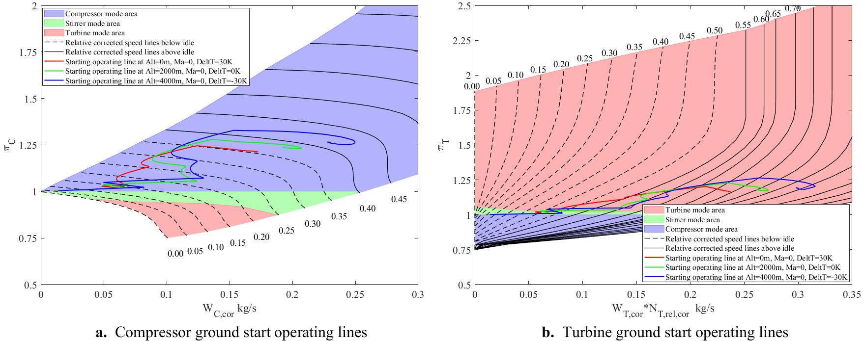
From Figure 12, it is evident that under all inlet conditions, the compressor’s operating point remains within the compressor mode region, while the turbine’s operating point initially falls within the stirring mode region during the early stages of the start process, and then enters the turbine mode region, which corresponds to the expected operating modes of the compressor and turbine during a ground start. Additionally, with increasing inlet altitude and decreasing temperature deviation, the total inlet temperature of all components decreases, causing the relative corrected speed to rise, thereby shifting the start process operating line to the right.
In conclusion, the curve- and surface-fitting-based extrapolation method proposed in this study for sub-idle component characteristics can fully utilize known data when only above-idle corrected flow, pressure ratio, and isentropic efficiency characteristics are available. The extrapolated results cover all operating modes of the components. The simulation results demonstrate that the extrapolation method satisfies the requirements for conducting ground start simulations of aeroengines under different inlet conditions, further proving the method’s validity and usability.
4. Conclusions
In order to fully utilize the limited available data for extrapolating the characteristics of components below idle, while ensuring that the extrapolated results are reasonable and adequately reflect the unique operating modes of the components, a method for extrapolating component characteristics below idle based on curve and surface fitting is proposed. The main features of this method are as follows:
1. Curve and surface fitting are applied to the component characteristics above idle, and the extrapolated results are used to derive the characteristics below idle;
2. The use of the enthalpy change coefficient for extrapolation instead of directly extrapolating the isentropic efficiency addresses the discontinuity of isentropic efficiency, allowing the extrapolated results to better reflect the unique operating modes of the components;
3. A series of constraints are applied to ensure the rationality of the extrapolated results.
For a specific micro turbojet engine, the proposed extrapolation method is used to obtain the component characteristics below idle, given only the characteristics above idle for the compressor and turbine. The extrapolated results cover all operating modes of the compressor and turbine. By importing these extrapolated results into the component-level model, a successful simulation of the ground start process under different inlet conditions was achieved, thus validating the rationality and usability of the extrapolated results. Therefore, the proposed extrapolation method addresses the shortcomings of existing methods, such as high data requirements, inability to fully utilize available data, and inability to adequately reflect the unique operating modes of the components, and meets the need for simulating the ground start process of turbojet engines under different inlet conditions.
5. Patents
The method employed in this study has been filed for a patent in China under the title: "A Method for Extrapolating Characteristics of Aero-Engine Components Below Idle Speed Based on Curve Fitting and Surface Fitting" (Patent Application No. CN202410578419.9). The first and second inventors listed on the patent application is the same as the first author and second (corresponding) author of this paper, respectively. Currently, the patent application is under review and has not yet been granted.
Author Contributions
All authors contributed to this work. Y.C. proposed the method described in this study, handled data processing and analysis, conducted simulation validation, drafted the manuscript, and revised it. T.Z. provided guidance during the development of the method, simulation validation, and manuscript revision. Z.C., Y.A.-Y. and E.T. assisted in refining the model functionality and reviewed the manuscript.
Data Availability Statement
Some or all data, models, or codes that support the findings of this study are available from the corresponding author upon reasonable request.
Conflicts of Interest
The authors declare no competing interests.
Abbreviations
The following abbreviations are used in this manuscript:
| PCHPI | Piecewise Cubic Hermite Polynomial Interpolation |
References
- Jones, G.; Pilidis, P.; Curnock, B. Extrapolation of Compressor Characteristics to the Low-Speed Region for Sub-Idle Performance Modelling. In Proceedings of the Volume 2: Turbo Expo 2002, Parts A and B; ASMEDC, Amsterdam, The Netherlands, 1 January 2002; pp. 861–867. [Google Scholar] [CrossRef]
- Kurzke, J. How to Create a Performance Model of a Gas Turbine from a Limited Amount of Information. In Proceedings of the Volume 1: Turbo Expo 2005; ASMEDC: Reno, Nevada, USA, January 2005; pp. 145–153. [CrossRef]
- Shi, Y. A Research on full states performance model for civil high bypass turbofan engine. Thesis for Doctor’s Degree of Northwestern Polytechnical University, 2017.
- Agrawal, R.K.; Yunis, M.A. A generalized mathematical model to estimate gas turbine starting characteristics. in Volume 1: Journal of Engineering for Power, 1982, 104, 194-201. [CrossRef]
- Sexton, W.R. A method to control turbofan engine starting by varying compressor surge valve bleed. Thesis for Master’s Degree of Virginia Polytechnic Institute and State University, 2001.
- Gaudet, S.R.; Gauthier, J.E.D. A Simple Sub-Idle Component Map Extrapolation Method. In Proceedings of the Volume 1: Turbo Expo 2007; ASMEDC: Montreal, Canada, 1 January 2007; pp. 29–37. [CrossRef]
- Zhou, W.X. Research on object-oriented modeling and simulation for aeroengine and control system. Thesis for Doctor’s Degree of Nanjing University of Aeronautics and Astronautics, 2006.
- Rao, G.; Su, S.M.; Zhai, X.B. Method of compressor characteristic extension combining exponent extrapolation method with support vector machine. Journal of Aerospace Power 2017, 32, 749–755. [CrossRef]
- Hao, W.; Wang, Z.X.; Zhang, X.B.; Zhou, L.; Wang, J.K. Ground starting modeling and control law design method of variable cycle engine. Journal of Aerospace Power 2022, 37, 152–164. [Google Scholar] [CrossRef]
- Hao, W.; Wang, Z.X.; Zhang, X.B.; Zhou, L.; Wang, W.L. Modeling and simulation study of variable cycle engine windmill starting. Journal of Propulsion Technology 2022, 43, 44–54. [Google Scholar] [CrossRef]
- NASA Aerodynamic design of axial flow compressors. Preprint at. Available online: https://ntrs.nasa.gov/api/citations/19650013744/ downloads/19650013744.pdf.
- De-You, Y. Modelling the Axial-Flow Compressors for Calculating Starting of Turbojet Engines. In Proceedings of the Volume 1: Aircraft Engine; Turbomachinery; American Society of Mechanical Engineers: Beijing, People’s Republic of China, September 1 1985; p. V001T02A038. 001. [CrossRef]
- Ju, X.X.; Zhang, H.B.; Chen, H.Y. A research on start-up modeling for turbo shaft engines. Journal of Propulsion Technology 2017, 38, 1386–1394. [Google Scholar] [CrossRef]
- Steinke, R.J. A computer code for predicting multistage axial-flow compressor performance by a meanline stage-stacking method. Preprint at. 2020. Available online: https://ntrs.nasa.gov/api/citations/19820017374/downloads/19820017374.pdf.
- Zachos, P.K.; Aslanidou, I.; Pachidis, V.; Singh, R. A Sub-Idle Compressor Characteristic Generation Method With Enhanced Physical Background. Journal of Engineering for Gas Turbines and Power 2011, 133, 081702. [Google Scholar] [CrossRef]
- Zachos, P.K. Gas turbine sub-idle performance modelling; altitude relight and windmilling. Thesis for Doctor’s Degree of Cranfield University, 2010.
- Zheng, J.; Chang, J.; Ma, J.; Yu, D. Modeling and Analysis of Windmilling Operation during Mode Transition of a Turbine-Based-Combined Cycle Engine. Aerospace Science and Technology 2021, 109, 106423. [Google Scholar] [CrossRef]
- Ferrer-Vidal, L.E.; Iglesias-Pérez, A.; Pachidis, V. Characterization of Axial Compressor Performance at Locked Rotor and Torque-Free Windmill Conditions. Aerospace Science and Technology 2020, 101, 105846. [Google Scholar] [CrossRef]
- NASA Extended parametric representaion of compressor fans and turbines Volume I—CMGEN user’s manual. Available online: https://ntrs.nasa.gov/api/citations/19860014465/downloads/19860014465.pdf.
- NASA Extended parametric representaion of compressor fans and turbines Volume II—PART user’s manual. Available online: https://ntrs.nasa.gov/api/citations/19860014466/downloads/19860014466.pdf.
- NASA Extended parametric representaion of compressor fans and turbines Volume III—MODFAN user’s manual. Available online: https://ntrs.nasa.gov/api/citations/19860014467/downloads/19860014467.pdf.
- Shi, Y.; Tu, Q.Y.; Yan, H.M.; Jiang, P.; Cai, Y.H. A full states performance model for aeroengine. Journal of Aerospace Power 2017, 32, 373–381. [Google Scholar] [CrossRef]
- Wang, J.M.; Guo, Y.Q.; Yu, H.F. Extension method of engine low speed characteristics based on backbone features. Journal of Beijing University of Aeronautics and Astronautics 2023, 49, 2351–2360. [Google Scholar] [CrossRef]
- Jun, F.; Tianhong, Z. Simulation of Start-Up Process of Turbofan Engine Based on Full-State Characteristics of Fan. 41. [CrossRef]
- Kurzke, J. SmoothC9: Preparing compressor maps for gas turbine performance modeling. User’s Manual. Available online: https://www.gasturb.com.
- Kurzke, J. SmoothT9: Preparing turbine maps for gas turbine performance modeling. User’s Manual. Available online: https://www.gasturb.com.
- Kurzke, J. Correlations Hidden in Compressor Maps. In Proceedings of the Volume 1: Aircraft Engine; Ceramics; Coal, Biomass and Alternative Fuels; Wind Turbine Technology; ASMEDC: Vancouver, British Columbia, Canada, January 1 2011; pp. 161–170. [CrossRef]
- Kurzke, J. Generating compressor maps to simulate starting and windmilling. International Society for Air Breathing Engines 2019, 2499. [Google Scholar]
- Joachim, K. Turbine Map Extension—Theoretical Considerations and Practical Advice. J. Glob. Power Propuls. Soc. 2020, 4, 176–189. [Google Scholar] [CrossRef]
- Joachim, K. Starting and Windmilling Simulations Using Compressor and Turbine Maps. J. Glob. Power Propuls. Soc. 2023, 7, 58–70. [Google Scholar] [CrossRef]
- Kurzke, J. An enhanced compressor map extension method suited for spool speeds down to 1%. J. Glob. Power Propuls. Soc. 8, 215-226 (2024). [CrossRef]
- Kurzke, J. How to Get Component Maps for Aircraft Gas Turbine Performance Calculations. In Proceedings of the Volume 5: Manufacturing Materials and Metallurgy; Ceramics; Structures and Dynamics; Controls, Diagnostics and Instrumentation; Education; General; American Society of Mechanical Engineers: Birmingham, UK, June 10 1996; p. V005T16A001. [CrossRef]
Figure 3.
Fitting and extrapolation result of compressor maximum and minimum pressure ratio.
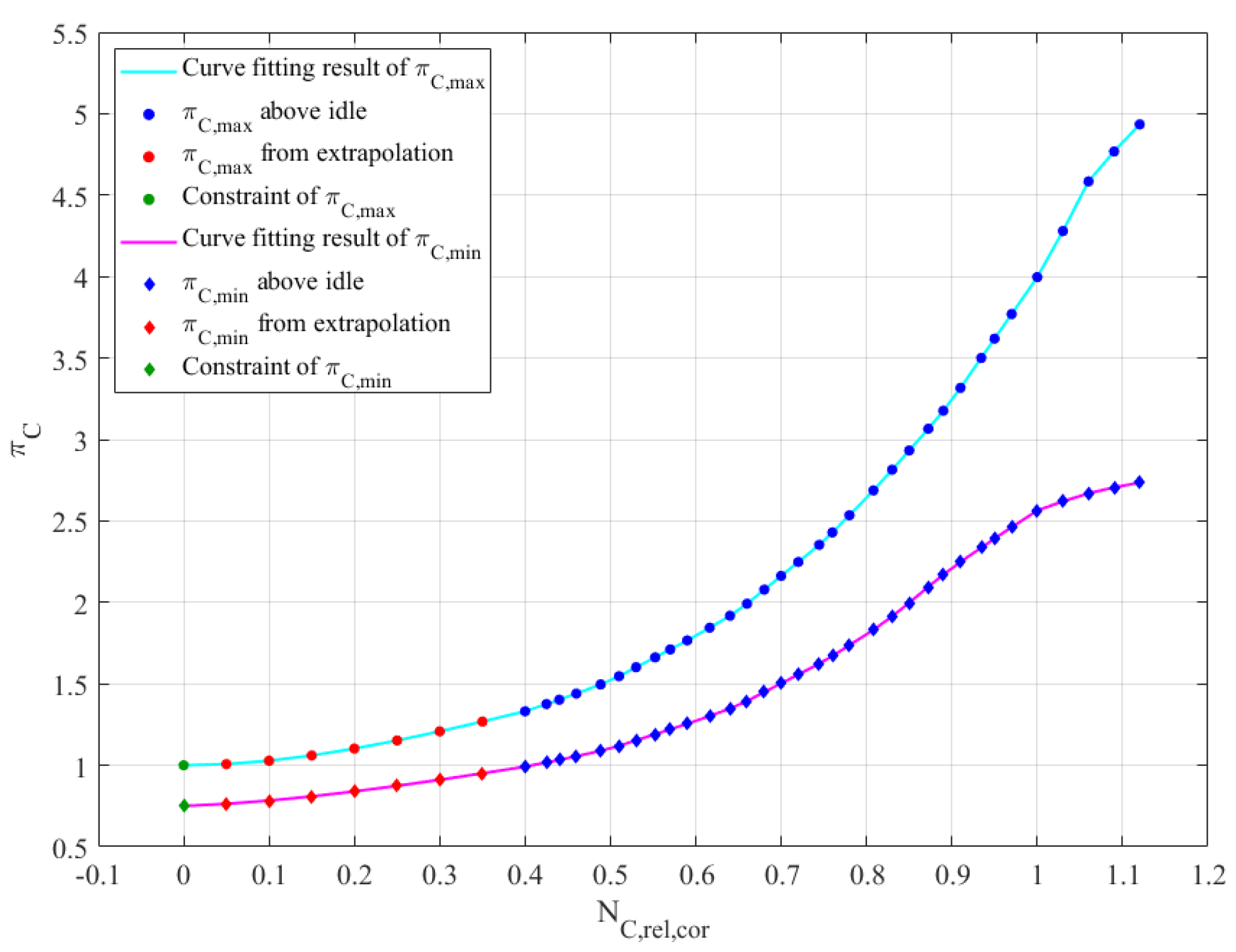
Figure 4.
Fitting and extrapolation result of compressor corrected flow rate.
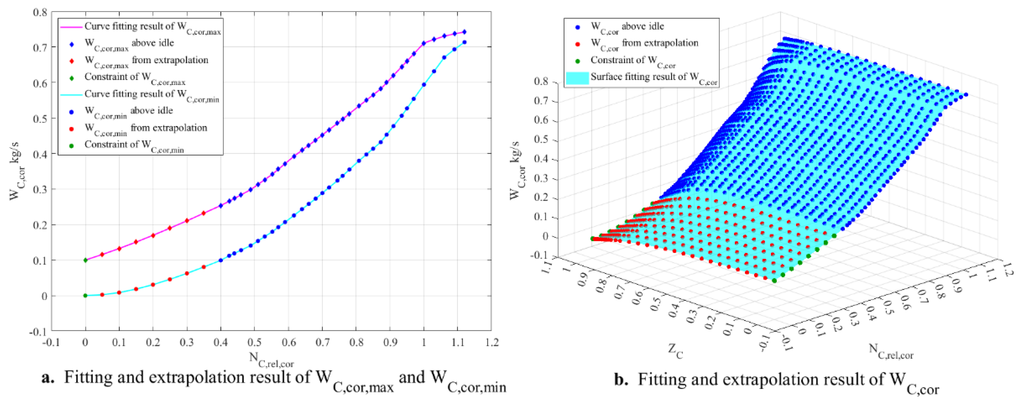
Figure 5.
Fitting and extrapolation result of compressor specific enthalpy change coefficient.
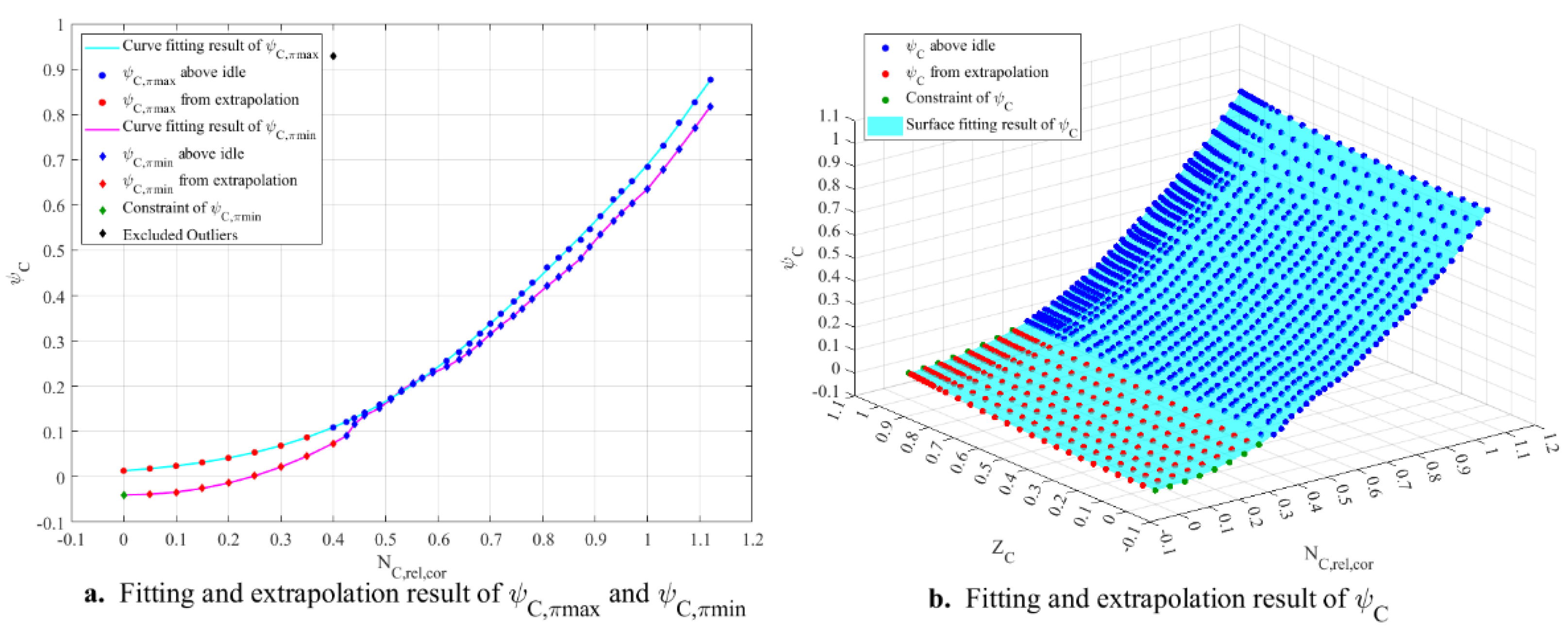
Figure 6.
Fitting and extrapolation result of turbine maximum and minimum pressure ratio.
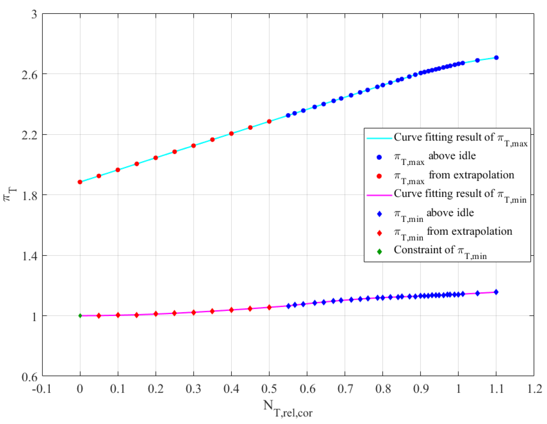
Figure 7.
Fitting and extrapolation result of turbine corrected flow.
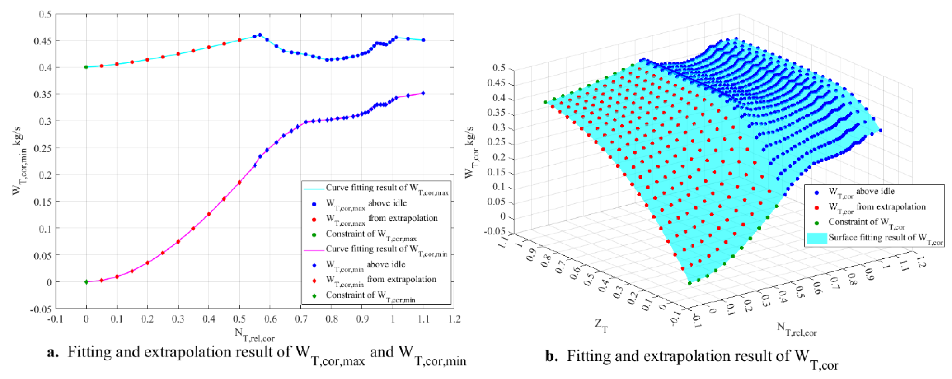
Figure 8.
Fitting and extrapolation result of turbine specific enthalpy change coefficient.
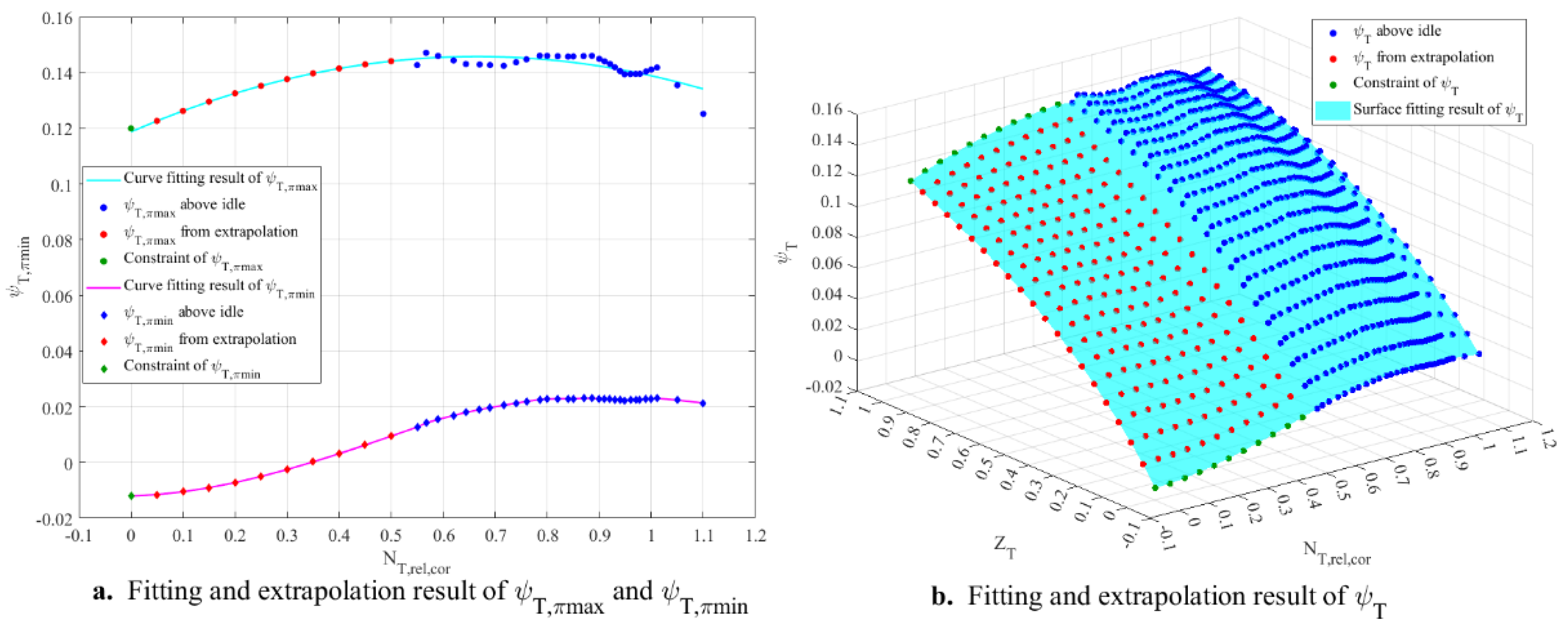
Figure 9.
Compressor characteristic maps after extrapolation.
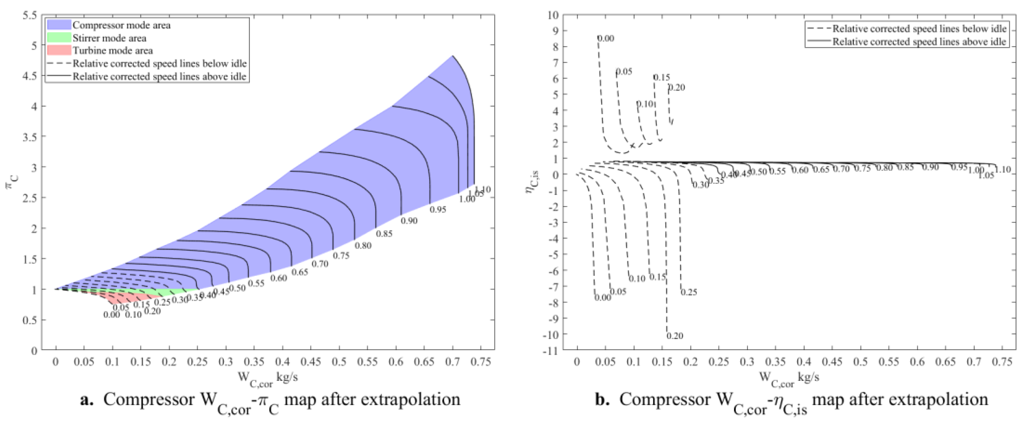
Figure 10.
Turbine characteristic maps after extrapolation.
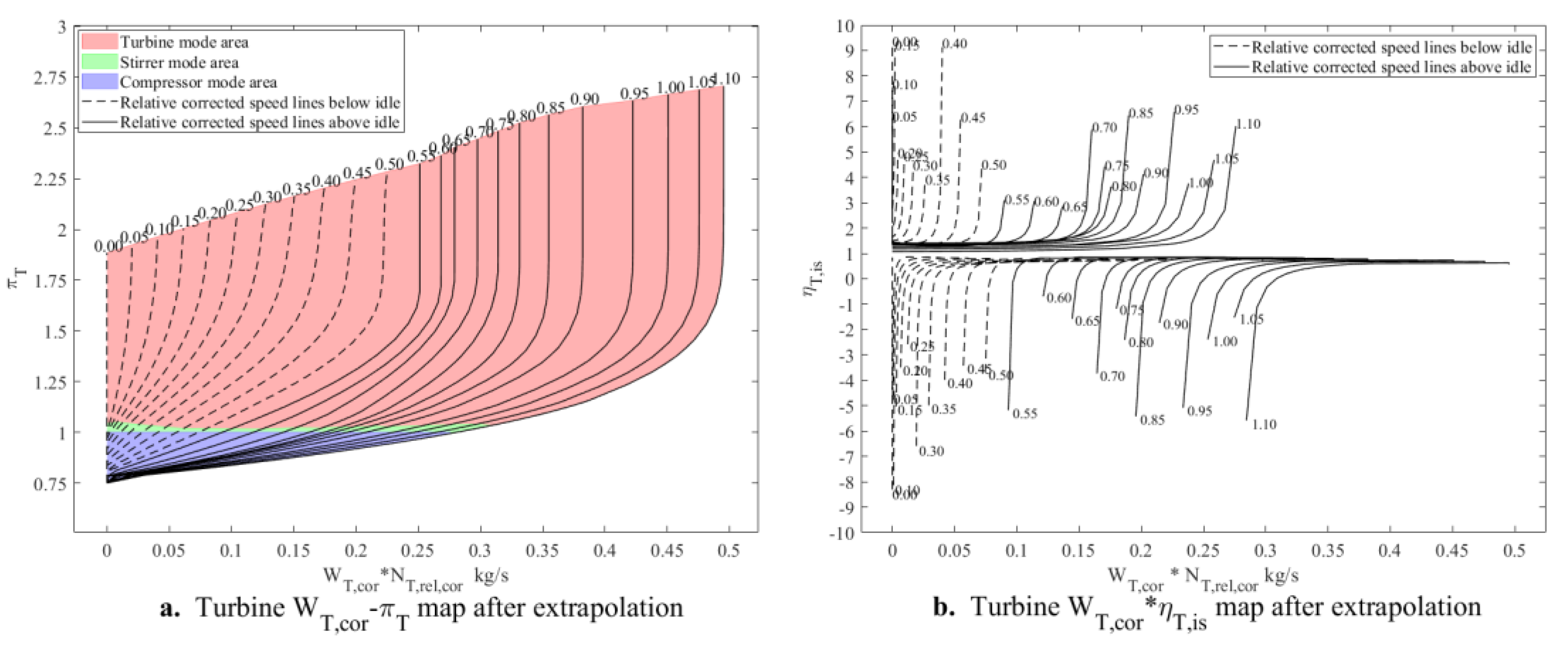
Figure 11.
Ground start simulation result. (Pt3: Compressor outlet total pressure, Tt5: Turbine outlet total temperature)
Figure 11.
Ground start simulation result. (Pt3: Compressor outlet total pressure, Tt5: Turbine outlet total temperature)
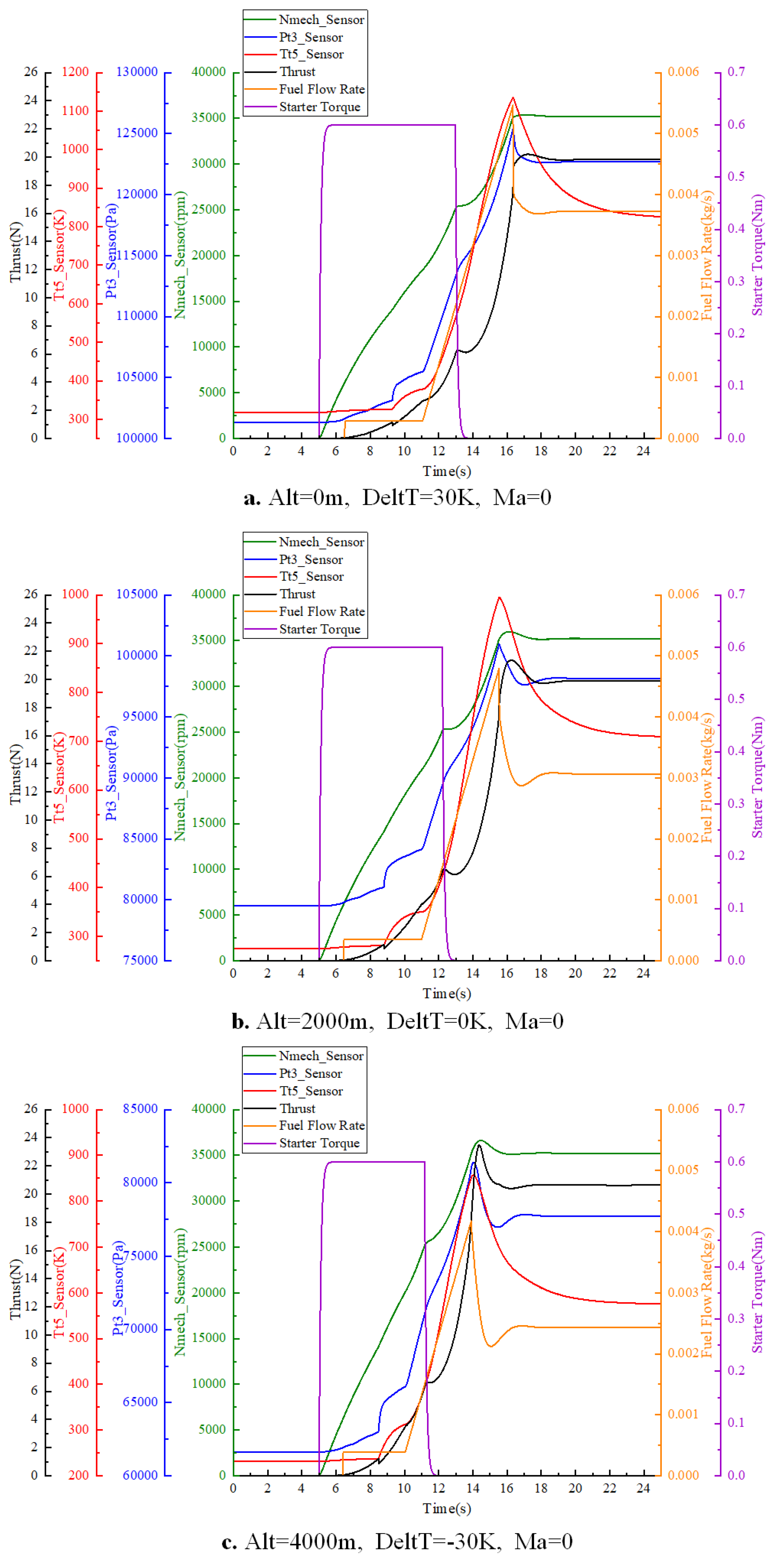
Figure 12.
Ground start operating lines.
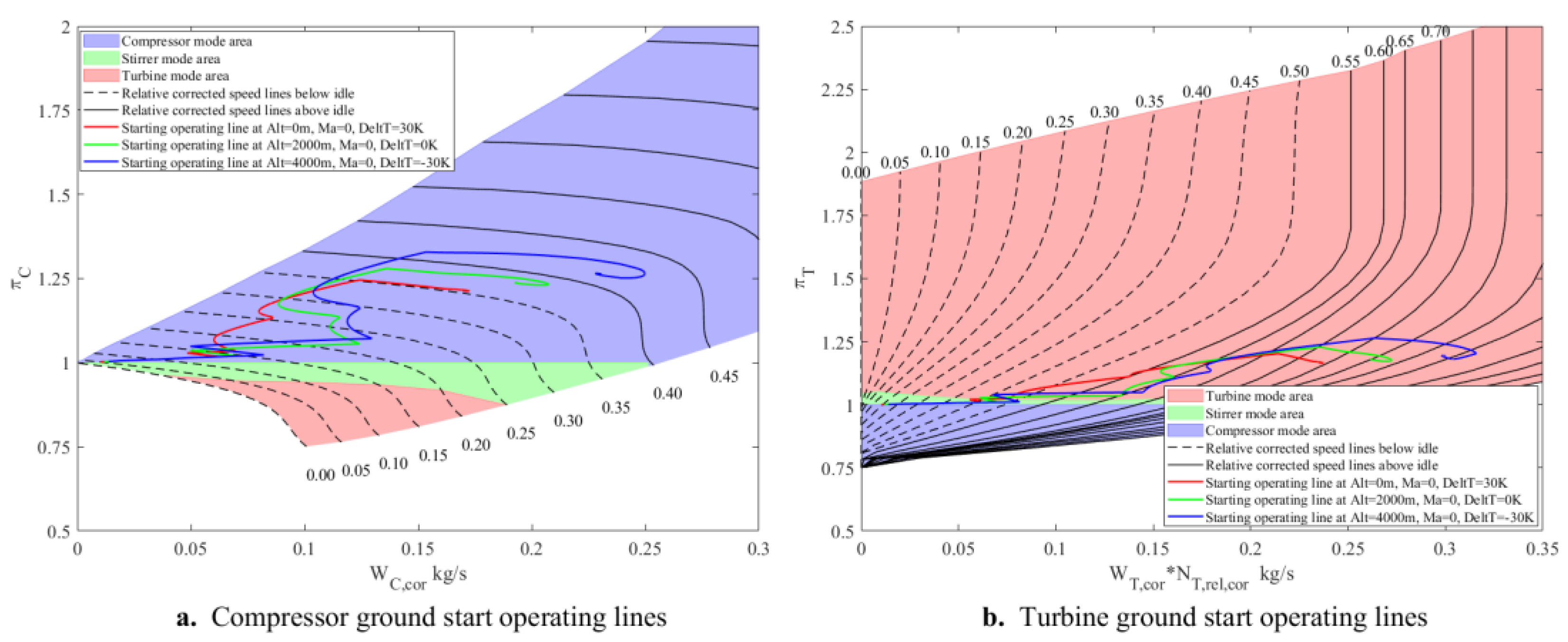

Table 1.
Design point parameters of a micro-turbojet engine.
| Mass Flow Rate (kg/s) | Compressor Pressure Ratio | Turbine Outlet Total Temperature (K) | Shaft Speed (rpm) | Thrust (N) |
|---|---|---|---|---|
| 0.692 | 3.39 | 1165.49 | 97070 | 351.71 |
Disclaimer/Publisher’s Note: The statements, opinions and data contained in all publications are solely those of the individual author(s) and contributor(s) and not of MDPI and/or the editor(s). MDPI and/or the editor(s) disclaim responsibility for any injury to people or property resulting from any ideas, methods, instructions or products referred to in the content. |
© 2025 by the authors. Licensee MDPI, Basel, Switzerland. This article is an open access article distributed under the terms and conditions of the Creative Commons Attribution (CC BY) license (http://creativecommons.org/licenses/by/4.0/).
Copyright: This open access article is published under a Creative Commons CC BY 4.0 license, which permit the free download, distribution, and reuse, provided that the author and preprint are cited in any reuse.


