
Submitted:
07 April 2025
Posted:
08 April 2025
You are already at the latest version
Abstract
This study was conducted in a temperate-continental city of Europe (Timișoara, Romania) and aimed to investigate the contribution of urban vegetation in maintaining air quality and mitigating the heat in the analyzed city. It was studied The Central Park „Anton von Scudier” located in the downtown of Timișoara City (45°45′05″N, 21°13′16″E) for the following air parameters: fine particulate matter PM2.5 (aerodynamic diameter < 2.5 μm), fine particulate matter PM10 (aerodynamic diameter < 10 μm), AQI (Air Quality Index) (resulted from PM2.5 and PM10), particles number, air temperature, air relative humidity, TVOC (total volatile organic compounds), HCHO (formaldehyde). Nine sample points of air monitoring were established: seven inside the green space and two outside it. The air monitoring was done in the late August, in four consecutive working days (Monday-Thursday), within 12:00-14:00 a.m. The air measurements were made using a portable device for outdoor air monitoring (Temtop LKC-1000 Series Air Quality Monitor). The results of this study show that urban vegetation remains a reliable factor in reducing PM2.5 and PM10 in cities air and in keeping the AQI within the limits corresponding to good air quality, but also that air relative humidity counteracts the contribution of vegetation in achieving this goal. Thus, the study highlights the importance of air humidity in enhancing the values of PM2.5, PM10, AQI, and in exceeding their admissible or recommended limits for air quality. There was not confirmed by this study the effect of wet deposition of the airborne particles as effect of precipitations. Inside the park, the HCHO concentration increased by up to 4-5 times compared to the outside, and this increase was not caused by vehicle traffic, but rather by the photochemical reactions generating HCHO. Regarding the cooling effect on air temperature, the studied green space did not exhibit this effect, as the air temperature inside it increased by up to 1-6°C compared to the outside, which means it did not achieved its goal of providing climatic comfort to citizens during the summer and serving as a cooling spot in the city. Our results contrast the general perception and conviction that urban parks and green spaces are cooler islands within the cities and draw attention to the fact that having a green space in a city does not necessarily mean achieving environmental goals, such as reducing the heat risk of cities. In this study, based on the results, we consider that the main limitations in achieving these objectives were the park’s small size (88 hectares) and its morphology and architecture resulting from the integration of the species that compose it. It follows from these data that it is not enough that an urban green space to be established, but its design must be combined with urban morphology strategies if the heat mitigation effect is to be achieved and the cooling benefits are to be maximized in cities. Therefore, in the urban planning, the environmental strategies should comprise not only aesthetic criteria, but also scientific criteria in order to reach the final goal of the urban green spaces in the cities: a sustainable, healthy, and comfortable environment.
Keywords:
urban park
; urban ecosystem
; urban health
; urban resilience
; ecosystem services
; heat island
; urban pollution
1. Introduction
Urban green spaces represent the connection between humans and nature in cities. The way people’s emotional reactions are influenced by accessing green spaces, as well as the social consequences resulting from this connection, have been a topic of interest, especially in recent years. Surveys of the urban population have shown that city dwellers primarily access urban green spaces for reasons related to recreation and spending leisure time in an area with natural elements, but also because of need to access a cooler area during the summer, as well as because the belief that urban green spaces are, within cities, islands with clean air, or at least with cleaner air than the surrounding areas [1]. It follows from this that the general perception of city dwellers is that urban green spaces are places for recreation and means of ensuring air quality in cities, as well as thermal comfort in the context of climate change and urban warming so strongly felt in urban environments.
Policies to ensure air quality in areas human inhabited are diverse, but the nature-based ones are by far the most implementable and feasible, mainly due to the non-static and continuously dynamic nature of this environmental factor, which is why other remedial solutions are less applicable. It thus becomes evident that, on a global scale, the only truly viable option for ensuring air quality is self-purification, which involves the contribution of biological factors in achieving this result. Most studies on this topic have been conducted in urban environments, as these areas have multiple major sources of air pollution, and because a large part of the human population resides in cities (over 70% in Europe and America), and is predicted that by 2050, more than 70% of the world’s population will be urban [2]. The use of vegetation as a tool to obtain quality air in cities has been widely studied in many parts of the world [3,4,5]. Most of the studies approach many industrialized urban areas of the world with the aim to highlight the role of urban vegetation in providing ecosystem services that ensure urban air quality. Thus, the results of research in the field to date, have shown that urban vegetation, especially woody vegetation, is able to extract and sequester the atmospheric carbon dioxide and to retain and trap the airborne particulate matter or other air pollutants [6]. Also, the urban vegetation can act like a protective barrier between pollutants and their sources and population [7]. To achieve these goals, numerous factors are decisive. Some of these are vegetation related, such as canopy size, leaf area and shape [7], stomata characteristics [7], trichomes presence [7], intercellular spaces available for gas diffusion in the case of gaseous pollutants [8], evapotranspiration, leaf architecture and morphology in generating the shading effect. However, other factors pertain to chemical and physical processes occurring both at the plant level and in its surrounding environment. Therefore, some approaches to the role of urban vegetation in ensuring air quality look at the impact on the adjacent microclimate [9] or on the local climate of the site. Thus, it results that the plant potential in pollution mitigation in urban areas is a species-specific mechanism. Urban studies have shown that plants have the ability to capture the atmospheric pollutants based on species-specific physiological and morphological characteristics that differentiate them in terms of efficiency, making them, from this point of view, more or less preferable for inclusion in urban green space planning. For example, some studies [10] have shown that mature trees with large canopy are major contributors in optimizing and regulating the ecosystem services in cities, while large and open urban green spaces with extensive natural vegetation provide multi-functionality in regulating services [11]. The leaf morphology and microstructure influence the retention patterns of the pollutants and also their removal with fallen precipitations or with wind. Therefore, in urban green planning, is important to select urban vegetation by estimating species contribution to air purification according to the meteorological conditions of the zone. The climatic patterns are also important. Several studies [12] have shown that, in the removal process of the pollutants from plant leaves, is more influencing the rainfall phase than other factors, such as particle diameter or particle adherence to the leaf. Meteorological conditions significantly influence the atmospheric pollution levels, affecting the dispersion, transport, and accumulation of pollutants. Essential meteorological factors that intervene in these processes include thermal inversions, wind speed and direction, atmospheric humidity, and precipitations. In the case of thermal inversions, if a warmer air layer is situated above a cooler, denser air layer that contains pollutants, it prevents the dispersion of pollutants and traps them in the lower layer, potentially increasing local pollution. Urban vegetation can mitigate this phenomenon by ensuring a more efficient local air circulation through evapotranspiration processes, by shading the ground, but also as an effect of the vertical disposition of individuals of different heights.
Wind speed and direction play an important role in the transport and dispersion of pollutants.
Strong winds help dilute and remove particulate pollutants, reducing their concentrations in a given area. However, strong winds can also cause surface erosion of buildings in cities, increasing levels of pollutants such as airborne particulate matter. Low wind speeds can also impact urban air quality by favoring air stagnation and keeping pollutants in certain areas for longer periods, resulting in a higher local exposure risk.
Besides the effect in pollutants capture and air phytoremediation, the urban vegetation can emit biogenic substances with supporting role in human healts, such as biogenic volatile organic compounds (VOC), strengthening public’s and authorities’ conviction of the necessity of having a reasonable area of green space per inhabitant in cities. World Health Organization (WHO) recommends a minimum surface of green space by 9 m2 per person and an ideal surface by 50 m2 per person [13], whereas considers as acceptable the physical accessibility of urban green spaces by residents within a short distance, a 5 minute walk or a distance up to 300 m. Also, for climatic purposes, WHO recommend a minimum width of green corridors by 50 m, ideally over 300 m [14].
Another important ecosystem service provided by urban green spaces is their critical role in mitigating the effect of urban heating, contributing thus to urban resilience. The urban resilience could be increased when, for establishing urban parks, are used the most suitable species [15] to reach this goal, such as native or alien species, species resistant to drought stress, or long-life species. The urban vegetation contributes to energy saving in cities by enhancing the thermal performance of the buildings [16] and representing thus an unconventional and sustainable solution of cooling in the dense populated areas.
The intrinsic relationship existing for long time between humans and nature generated their strong feeling of biophilia [17] towards other living beings in the global ecosystem, which also creates the special need of city dwellers to connect with nature through urban green spaces. Studies have shown the psychological, emotional, and social benefits of urban green parks [18] for those who access them, through sensory experiences and interactions (visual, auditory, olfactory, and even tactile) that benefit human health and wellbeing.
In light of the above exposed arguments, the research aimed to investigate the contribution of an urban green space in maintaining air quality and mitigating the warming in a Romanian city, as related to its surrounding environment, in order to reveal the ecosystem services provided by the urban green spaces in urban areas. This study brings data about the importance of the green spaces in the urban matrix and about the ecosystem services provided by urban vegetation. The results highlight that urban vegetation is a reliable factor in maintaining air quality, but also draw attention to the fact that simply having green spaces in cities does not necessarily mean achieving environmental objectives, such as reducing the urban heat risk, therefore urban morphology strategies must be implemented to maximize cooling benefits and effectively mitigate heat.
2. Materials and Methods
2.1. Research Site
The research was carried out in the Central Park „Anton von Scudier” in downtown Timișoara (Figure 1), Romania (45°45′05″N, 21°13′16″E).
This urban green space has a temperate-continental climate, covers an area by 87,663 m², and is one of the oldest parks in Timișoara, being established in 1880 by order of General Anton von Scudier (an Austro-Hungarian officer of German origin who served as a military governor of Timișoara, known for his military career and contributions to the city’s development, and who lived between 1818 and 1885). This study monitored 9 sample points (SP) noted as SP1, SP2, SP3, SP4, SP5, SP6, SP7, SP8, and SP9. These sample points were established in relation to the park’s boundary line, as follows: SP1 – outside park, at 93 m from park border; SP2 – outside park, at 55 m from park border; SP3 – on the park border; SP4 – inside park, at 10 m from border; SP5 – inside park, at 20 m from border; SP6 – inside park, at 30 m from border; SP 7 – inside park, at 164 m from border; SP8 – inside park, at 275 m from border; SP9 – outside park, at 583 m from border. The sample point SP9 was chosen at a greater distance from the park because it was aimed for it to be located both far from vegetation and enclosed by buildings, to determine if there are similarities or differences in the monitored parameters between the vegetated-environment and the built-up, vegetation-free environment.
2.2. Research Methodology
Air quality monitoring was conducted over four consecutive days at the end of August, from August 19 to August 22, 2024 (working days, Monday to Thursday), between 12:00 and 14:00, at nine fixed points (Figure 1). The monitoring days were labeled as Day 1, Day 2, Day 3, and Day 4. The measurements were performed using the device Temtop LKC-1000 Series Air Quality Monitor [19]. This is an air quality monitoring tool, a low-cost sensor capable of measuring a variety of essential parameters for the assessment of environmental conditions. Low-cost sensors provide real-time air monitoring and highly localized air information, and, despite their low cost, accurate information [20]. Also, low-cost and accessible instruments [21,22,23] and at the same time portable [23,24] have shown to be reliable in air quality monitoring. The instrument used for this research was suitable for the intended purpose because it uses high-precision sensors and has a compact size (177×65.5×32 mm), which makes it conveniently portable, and regarding the operating conditions, the device functions optimally at temperatures ranging from 0 to 50°C and at an air relative humidity of 0 to 90%. Additionally, the device is designated to operate at standard atmospheric pressure (1 atm). The following air parameters were monitored with this device: fine particulate matter PM2.5 (with aerodynamic diameter <2.5 μm), fine particulate matter PM10 (with aerodynamic diameter <10 μm), air temperature, air relative humidity, TVOC (total volatile organic compounds), HCHO (formaldehyde). As well, the Air Quality Index (AQI) and the particles number were monitored, both being indicators derived from the corroboration of the values recorded for PM2.5 and PM10. The Air Quality Index (AQI) is an indicator used to communicate air quality to the public in a format easily understood by a wide audience. The Temtop LKC-1000 Series Air Quality Monitor measures the particles number as an air indicator different from the sum of particles PM2.5 and PM10, because it also includes particles of other, smaller sizes. Although the detailed specifications regarding the exact size range of particles detectable by this device are not stated in the supplied specifications, in general, similar laser sensors can detect particles ranging from approximately 0.3 µm to 10 µm [25]. This does not mean that we know the exact size range the device used in this research is capable of measuring, but it suggests that it may measure particles smaller than those in the PM2.5 and PM10 categories, i.e., very fine particles.
The device was used to measure air parameters at the same height from the ground (approximately 1 meter above the ground) on all four days, and samples were taken from the same point each day. Three samples were taken from each point at equidistant time intervals, every 2 minutes (the device operated for 2 minutes, after which it was paused to record the data). The monitored parameters and the measurement characteristics of the air quality monitor (measurement range and resolution) are presented in Table 1.
2.3. Results Interpretation
For the interpretation of the recorded values, there are multiple assessment scales. The device used reports the recorded data with reference to the standards of the United States Environmental Protection Agency (EPA) only for the parameters PM2.5, PM10 and AQI (Table 2) [26], while for the parameters TVOC and HCHO, it follows the Air Quality Guidelines of the World Health Organization (WHO) (Table 3) [26,27]. However, for interpreting the results obtained in this study, to ensure consistency in interpretation and because WHO standards are more restrictive and therefore more relevant for assessing the impact of the measured values on human health (compared to Romanian standards in Table 2 and Table 3), it was decided that reporting the analyzed parameters to the WHO-recommended standards would be more appropriate (exception air temperature, air relative humidity and AQI, this last one being interpreted according to EPA standards - Table 2) [27,28].
For the interpretation of HCHO and TVOC values, some clarifications are necessary. WHO provides recommendations for maximum permissible limits for HCHO only for indoor air (Table 3) [27], while for TVOC, it recommends a range of 0.3-0.5 mg/m³ [27]. In Romania, there is legislation that regulates permissible limits for HCHO in the air (Law No. 104 of 15 June 2011) [29], which aligns with European Union standards (Directive 2004/107/EC of the European Parliament and of the Council of 15 December 2004) [30]. According to this European directive, the annual concentration limit for HCHO in the air is 0.1 mg/m³ (equivalent to 100 µg/m³), i.e. the same as that recommended by the WHO (Table 3) and the value to which the measured HCHO levels in this study were referenced. This value represents the maximum permissible long-term concentration of HCHO in the air over a period of one year. If this limit is exceeded in the long term, adverse effects on human health may occur, and public health protection measures must be implemented. Regarding TVOC, there is no specific national regulation in Romania that imposes a certain limit in outdoor ambient air, similar to the limits for PM10 and PM2.5, or for HCHO. However, European regulations (Directive 2008/50/EC of the European Parliament and of the Council of 21 May 2008) [31] influence the monitoring and management of TVOC emissions in the air, and these are applicable in Romania under environmental legislation. But, this directive also does not specify a certain concentration threshold for TVOC in the air. However, since TVOCs are considered a group of chemical pollutants that can affect human health, they are monitored within the air quality monitoring system, and the interpretation of this parameter’s values is made according to WHO recommendations (Table 3).
Regarding AQI, Romania does not have specific legislation regulating precise values for this air parameter. However, AQI is a concept used to assess air quality, and it is also utilized in Romania to inform the public about pollution levels and associated risks through various platforms. The AQI is an air quality index with multiple calculation methods across different countries. In this study, the AQI measured by the Temtop LKC-1000 device is derived exclusively from the measured PM2.5 and PM10 values, and its interpretation was made according to WHO standards (Table 2).
As for the total number of particles measured by the Temtop LKC-1000 Series Air Quality Monitor used in this study, there is no standardized maximum allowable limit expressed in particles per liter of air (pcs/L). This is because air quality standards typically focus on the mass of suspended particles (PM2.5 and PM10), expressed in µg/m³. The limit values for interpreting PM2.5 and PM10 levels therefore refer to particle mass and not to the total number of particles. Since the number of particles and their mass do not have a simple direct relationship (as particles of different sizes contribute differently to the total mass), there are no regulated standards for the total number of particles per liter of air. Regarding particulate matter, the PM2.5 and PM10 limit values for ambient air quality in force in Romania (according to Law No. 104 of 15 June 2011) (Table 2) were not considered in this study. This is because they are less stringent than those recommended by WHO, and we believe they downplay the concern that should be maintained regarding ambient air quality for the protection of human health.
Measurements were conducted over four consecutive weekdays to capture periods of intense human activity, at the same time intervals, at the same height, and in the same locations, allowing for the observation of the evolution and modification of the analyzed parameters. Since weather conditions varied on certain days, they were taken into account in the interpretation of results. Pearson correlations (p<0.05) were analyzed to determine whether the measured factors influenced each other and whether any relationships existed between them. Additionally, statistically significant differences (Paired-samples t-test, p<0.05) were examined between the recorded values at different depths within the park and outside of it. Graphs were created using Microsoft Office Excel (2010), and statistical analysis was performed using IBM SPSS Statistics version 28.0.
3. Results and Discussion
The measured values of the air parameters are presented in Table 4, by monitoring days and sample points (SP1-SP9).
3.1. Particulate Matter PM2.5
It was observed that in the first day of monitoring, for PM2.5, there is a decreasing trend in its concentration as one moves deeper into the park (Figure 2). The measurement points SP1 – SP2 are located outside the park, in areas with high traffic and car congestion, and they served as control points against which the recorded values were compared. Thus, the measurement point SP3 is located right at the edge of the park, at the park entrance, and it is the first point where a significant decrease in PM2.5 is observed on Day 1 compared to the SP1 and SP2 points, with reductions of 22.92% and 29.3%, respectively (Figure 2)
As entering deeper into the park, oscillations in PM2.5 values are observed, but the overall trend is a decrease compared to the values measured outside the park. At a distance of 20 meters inside the park (SP5), it was found that PM2.5 values had decreased by 42.76% compared to the more distant exterior point (SP2) located 55 meters away from the park boundary. A point of interest was located in the middle of the vegetation, 275 meters from the park entrance (SP8), where a significant decrease in PM2.5 values was observed compared to the park’s exterior (SP2) (Table 5), specifically a reduction of 48.66% (Figure 2), meaning a substantial decrease, almost half of the concentration outside the park. We consider this effect is due to the presence of tree vegetation in the park, related to which other studies have shown that higher levels of urban green space are associated with decreased pollution levels [21,32].
Some studies have shown that when aiming to avoid high concentrations of PM2.5, it is not enough to have urban parks with vegetation; it is essential for these parks to contain trees [33]. However, there are also studies [34,35] indicating that in cities, PM2.5 reduction has also occurred in built-up areas where the presence of buildings limits air ventilation and, consequently, air currents, suggesting that, at least from a physical perspective, buildings can serve as a physical source of limitation for PM2.5 concentrations. This is supported by the results of this study, as it was observed that, at the monitoring point SP9, located 583 meters from the park in a square surrounded by buildings and devoid of vegetation, PM2.5 concentrations were 31.37% lower compared to the exterior of the park, which is not bordered by buildings and lacks vegetation (SP2). This effect is comparable to the one recorded at the park entrance (SP3). When interpreting this result, we must also consider that the points SP1, SP2, and SP9 share the characteristic of being located outside the studied urban park. However, they differ in that at SP9, access by vehicles is restricted, whereas at SP1 and SP2, vehicle traffic is intense. Other major sources for airborne particulate matter (such as industrial sources) were not considered, because the research site was located in the downtown of the city, without industrial objectives. Only the plant pollen could be a source [36,37] or the aeolian erosion of buildings, but these were as well excluded due to the seasonal moment of the monitoring and local meteorological conditions in the monitoring days. Regarding the presence of the cars, a study conducted in another city in Romania [38] showed that the noise produced by them plays an important role in the propagation of the particulate matter along with the sound, because the vehicle-related noise penetrates the atmosphere and the airborne particulate matter formed at the noise source are ulteriorly lifted in the atmosphere by the sound waves. The same study also showed that vehicles are responsible for raising dust particles into the atmosphere through the rolling of their tires. Therefore, we consider that the higher PM2.5 values recorded at the exterior points SP1 and SP2 compared to the exterior point SP9 are also due to this factor (vehicle traffic), not just the absence of a mechanical barrier provided by buildings. However, these results also highlight the importance of urban morphology and architecture in achieving goals related to air quality in cities.
On the second day of monitoring, it was observed that the evolution of PM2.5 concentrations was similar to that of the first day. On the night between Day 3 and Day 4, it rained, which we consider to be the cause of the significant increase in PM2.5 concentrations on Day 4 compared to the previous days (Figure 2, Figure 3). Thus, on Day 4, after the rain during the night, PM2.5 exceeded the daily maximum limit of 15 μg/m³ recommended by WHO [28] in almost all monitoring points, including inside the park (except for SP6 and SP8), situation that was not observed for any sample point on Day 1, and on Day 2 and Day 3 it was only observed at the point outside the park (SP1). Therefore, on Day 2, only at the point SP1 located outside the park was exceeded the limit recommended by WHO, and the same occurred on Day 3. The recorded results indicate that atmospheric humidity is a factor that counteracts the contribution of vegetation as a factor for reducing PM2.5 concentrations in the air. Although no statistically significant correlation was found between PM2.5 concentration and air relative humidity in the study (Figure 4, Figure 5, Figure 6 and Figure 7), significant statistical differences (Table 5) regarding these parameters confirm what other researchers have found, namely that there is a strong positive correlation between air humidity and the increase in PM2.5 concentration [39]. This suggests that, depending on the air humidity, both the quantitative variation of these particles and their deposition differ, as some studies have shown that PM2.5 particles are envelopped with a hydrolayer within the condensing process, which determines an increased deposition [24]. It results that the presence of PM2.5 particles in the atmosphere is influenced by atmospheric humidity and precipitation [22]. However, if we compare the PM2.5 concentration in the air on Day 4 at SP1 and SP9, i.e. the points farthest from the park and thus from the presence of vegetation, we observe that it increased significantly compared to the other points (Figure 2), which strengthens the idea that vegetation remains a reliable factor for reducing PM2.5 in the air.
The range of PM2.5 concentrations measured in the air varied between 4.96 μg/m³ (inside the park, Day 1, SP8 – at 275 m from the border, among trees) and 23.26 μg/m³ (outside the park, Day 4, SP1 – at 93 m from the border, after rain) (Table 4, Figure 3). Although these data show the extremes of the measurements and only punctually exceed the daily limit recommended by WHO (15 μg/m³), when analyzing Table 4, very high values of this air parameter are observed compared to other values recorded in other cities. For example, a similar study conducted in Dublin (Ireland) showed air values of PM2.5 by 6-7 μg/m³ [21], lower than those recorded in this study
The effect of vegetation caused the PM2.5 values recorded in this study to remain lower inside the park, with significant increases only on Day 4 after precipitation falling, when the relative humidity of the air also increased. The concentrations were more frequently elevated outside the park, even at lower relative humidity levels in the atmosphere.
3.2. Particulate Matter PM10
Regarding the PM10 particles, it was observed that the dynamics of their concentration over the 4 consecutive days of monitoring generally resemble the trend of PM2.5 concentrations, with a decreasing trend as entering further into the park. As with PM2.5 particles, the lowest concentration was recorded in all monitoring days at point SP8, located deep within the park and surrounded by vegetation. These findings are similar with others showing an inverse association of urban green space with PM2.5 and PM10 [40]. For example, compared to SP2, which is located outside the park and 55 meters from its border, the PM10 concentration at SP8, located in the heart of the vegetation, was 44.47% lower (Figure 8), a statistically significant difference (Table 5). None of the recorded PM10 concentrations exceeded the daily recommended limit of 45 μg/m³ set by WHO, nor the 50 μg/m³ limit enforced in Romania. As with PM2.5 particles, a significant increase (Table 5) in PM10 concentrations was observed on Day 4, following the precipitation that occurred overnight between Day 3 and Day 4.
3.3. Air Quality Index (AQI)
The AQI values measured during the four consecutive days of monitoring are presented in Figure 9. The device used in this study calculates the AQI index exclusively based on the concentrations of PM2.5 and PM10, which is why this indicator follows the trends of the two parameters that determine it. According to the EPA’s air quality standards, which specify a maximum AQI value of 50 for good air quality (Table 2), with no negative effects on the human population, it was found that, for this study, the AQI values indicated good air quality inside the park, except for Day 4, when the value was exceeded following the precipitation from the previous night, resulting in moderate air quality. At the monitoring point SP1, the farthest from the park and lacking the physical protection of buildings, but near vehicle routes, the AQI values for good air quality were exceeded on Days 2-4. Similarly, at SP9, between buildings and without vegetation, AQI values were exceeded on Days 3-4 (Figure 9), suggesting that proximity to an urban park, an area with vegetation, cannot fully compensate for the presence of vehicles that generate PM2.5 and PM10 particles.
Comparing Figure 2 and Figure 8, it results that the contribution of PM2.5 particles is more significant in determining AQI values, as the permissible concentrations for PM10 were not exceeded at any measurement point. Throughout the 4 days of monitoring, a decreasing trend in AQI values was observed at the inner points of the park (SP3-SP8) compared to the outer points (SP1, SP9). The SP8 point inside the park showed the lowest AQI values during the first two measurement days. In interpreting the AQI values, the relative humidity of the air at the time of measurement was also taken into account. Thus, it was observed that on days with higher humidity, inside the park, where tree vegetation is much denser, AQI values had an increasing trend, reflecting lower air quality compared to previous days with lower humidity (Figure 9, Figure 12), and similarly in the park's exterior. Therefore, the increase in AQI values was consistent on Day 4 compared to Day 1 at all sampling points, with the increase exceeding 50% in nearly all measurement points, except SP2 and SP6 (Figure 9). On Day 4, it was also found that AQI positively correlated with the relative humidity of the air in the park’s exterior at SP2 (Figure 7), and negatively at SP8, located deeper within the vegetation (Figure 7). Similar results were found by Zender-Świercz et al. (2024) [22], who observed that AQI positively correlates with air humidity, especially when its values place the air quality in the unhealthy and moderate range. These results highlight the importance of air humidity in enhancing the concentration values of several air quality parameters (PM2.5, PM10, AQI) and in exceeding their admissible or recommendable limits. Statistically significant correlations were found between AQI and the concentrations of PM2.5 and PM10 (Figure 4, Figure 5, Figure 6 and Figure 7), but these were expected, considering that the AQI measured by the device used in the study is the expression of these two indicators, and since similar findings have been made in other studies of the same kind [22]. However, AQI correlated more frequently with PM2.5 concentration than with PM10 concentration (Figure 4, Figure 5, Figure 6 and Figure 7), indicating that PM2.5 concentration carries more weight in determining its value.
3.4. Particles Number
The measurement of the particle count (pcs/L) in the air showed that inside the park, the number of particles was lower than outside throughout all 4 days (Figure 10). Similarly to other monitored indicators, on Day 4, after precipitation, the amount of particles in the air increased considerably compared to the previous days. Thus, at SP8, the point located the deepest within the vegetation, the particle count was the lowest compared to other inner points of the park; however, here, on Day 4, it was 64.73% higher than on Day 1, a significant and noteworthy difference (Table 5). These results highlight both the importance of vegetation and the impact of meteorological conditions, in this case the relative atmospheric humidity resulting from the precipitation that fell the night before, on the amount and dynamics of particles in the air. Atmospheric humidity influences the composition and concentration of particles in the air. In conditions of high humidity, hygroscopic particles absorb water, leading to an increase in their size and changes in their physico-chemical properties. This process can have a dual effect: on one hand, it can facilitate the deposition and removal of pollutants from the atmosphere through wet deposition, and on the other hand, in the presence of fog or secondary aerosols, it can lead to the formation of fine liquid particles that contribute to an increase in their atmospheric proportion due to their suspension in the air for varying periods of time.
Among the meteorological variables, it was found that air relative humidity can predict the accumulation of particulate matter [41]. Results supporting the involvement of the same factors in the dynamics of particulate matter in the air have also been found and explained in the literature [42]. The vegetation of the studied park is predominantly represented by trees, which have been found to reduce the amount of particles in the air through retention mechanisms at the leaf level [43,44], absorption at the stomata level [44], or dispersion [45]. However, the situation observed on Day 4, when the particle concentration in the air increased significantly after the precipitation compared to previous days, was contradictory to the estimated expectations, as the wet deposition effect of the particles reported by other studies [24] was not confirmed.
3.5. Air Temperature
Temperature monitoring was also conducted on all four days and sample points taken for the study. The hypothesis and expectations underlying the research were that, as entering further into the park, the air temperature would decrease. These expectations were based on studies [46,47,48,49] showing that urban parks act as significant buffers against high temperatures during hot seasons. However, this hypothesis was not confirmed in the present study (Figure 11), as it was found that the air temperature was higher inside the park (SP3-SP8) than outside it (SP1, SP2, SP9) on almost all the days of measurement. Thus, the temperature differences between the park's exterior points and the interior points ranged from 1-6°C. A decrease in air temperature was observed on Day 4 compared to previous days, correlating with the rainfall the night before and the increase in relative humidity. Inside the park, the lowest air temperature was recorded at the point surrounded by tree vegetation, although this value remained approximately 2-3°C higher than the exterior of the park.
These results, similar to the variation in PM2.5 and PM10 particles, support the contribution of urban vegetation to influencing the dynamics of air quality parameters in urban areas. A higher air temperature inside an urban green space than outside it has been reported in other urban studies [33], and it can be explained by several hypotheses. One explanation might be that within the park, air ventilation through air currents is insufficient to reduce the air temperature, as happens outside it, and this fact could be influenced by the morphology of the surrounding environmental characteristics, such as vegetation structure and distribution [50], canopy porosity [51], landscape composition and morphology [49], and the presence and density of buildings [52,53], as well as alley and building albedo [54]. The monitoring point SP8, was surrounded by trees, and is possible that plant evapotranspiration to contribute to the increased of air humidity through aerosol formation, as this point had the highest relative humidity. Aerosols and water vapors in the air can absorb solar radiation, determining an increase in air temperature [55]. As well, air humidity can influence the rate of evapotranspiration of vegetation in the park, and if this process is reduced, its cooling effect on the ambient air temperature diminishes or is overtaken by solar radiation absorption [56,57]. Other interior sample points in the park (SP2-SP7) were near concrete alleys, so it’s possible that they released accumulated heat, thus increasing the air temperature. SP9 is situated in a square paved with concrete slabs and is lacked by vegetation, so it does not benefit from shading effects, as SP1 does, which is near a very tall building. Moreover, the presence of buildings can limit wind speed [58], and buildings and pavements absorb heat and release it, which could explain the additional 2-4°C observed at this point compared to other exterior points of the park (SP1 and SP2). It results from these data that it is not enough that an urban green space to be established, but its design must be integrated with urban morphology strategies if is aimed that the heat mitigation effect be achieved and maximized in cities. In addition, besides technical elements of urban design and those vegetation-related, importance should be given to the soils of the parks as related to their impact on local temperature increases. Some studies have shown that soil impermeability plays an important role in raising air temperature in urban green spaces [59]. Soils in urban parks, especially in urban arboreta, are minimally disturbed technosols due to maintenance work, and therefore their compaction degree and impermeability may be high. Therefore, it should pay attention to other factors involved in maintaining soil permeability in urban parks, such as pedofauna, since its contribution to the soil permeability was demonstrated [60,61,62]. No significant and consistent correlations were found in this study between air temperature and other parameters, as some other studies have shown. For instance, some studies have indicated that air pollution amplify the intensity of the urban heat island effect especially when the green spaces have small sizes [63], while other studies support this idea, showing a strong correlation between air temperature PM2.5 concentration [64] and that PM10 concentration increases when the temperature is low [65]. No significant positive correlation was found between air temperature and its relative humidity, meaning that other factors likely influenced the increase in air temperature inside the park compared to outside, possibly factors related to shading architecture [66], tree density [58], airflow [67], vegetation cover and layouts [68], or even alley surface materials. It is possible that the small size of the studied park (approximately 88 hectares) to be as well a factor which determined the increase of air temperature inside it compared to the outside, because it was found that larger parks with good vegetation (tree) coverage may better enhance the evapotranspiration rate and pollutant absorbtion, increasing thus their cooling effect [63]. A study [33] revealed that urban green spaces smaller than 525 hectares have a cooling effect only by approximately 1°C. Thus, our findings show the importance of the integrated urban green space design in maximizing the cooling benefits of the urban green spaces. This is aspect is very important when the urban park attendance is considered, as it may be affected [69] because people are specifically seeking the cooling effects of urban green spaces, and if this is absent, their thermal comfort level is not ensured.
3.6. Air Relative Humidity
The relative humidity of the air decreased as entering deeper into the park (Figure 12) compared to the exterior points SP1 and SP2. However, when comparing the exterior points of the park, it was observed that the one located between buildings showed a lower air relative humidity than those near the park. It is possible that the proximity to vegetation be the reason for the higher air relative humidity around it, due to the evapotranspiration effect [66]. Clearly, as a result of the precipitation that occurred during the night from Day 3 to Day 4, the relative humidity of the air increased on Day 4 both inside the park, with values ranging from 30.64% (SP7) to 37.76% (SP6), and outside, with values ranging from 28.03% (SP2) to 36.01% (SP1). It was found that, inside the park, the relative humidity of the air increased the most in the point where the trees become denser (SP8), surrounded by tree vegetation, likely as a result of the evapotranspiration effect exhibited by the plants. However, it still remained lower than the air relative humidity outside the park.
The decrease in relative air humidity as advancing towards the interior of an urban park can possibly be explained by the connection between plant evapotranspiration and local warming. Since in the studied urban green space the air temperature increased compared to the exterior, it is possible that the trees in the park release water vapor through transpiration, but this process may also be accompanied by the absorption of solar radiation by the water vapor or aerosols, thus causing the air temperature to rise. If the air temperature increases within the park due to the retention of heat as a result of this mechanism, for which we suspect as primary cause the inefficient circulation of air masses, then the relative humidity of the air decreases.
Thus, an inverse proportional relationship between air temperature and air relative humidity results. This relationship was not statistically validated in this study, but that does not mean it does not exist, especially since it has been reported by other researches. For example, it has previously been shown that the urban heat island effect is due to the lack of humidity [70], which determines an increase in air temperature, making cities warmer, and other studies have also found that increased atmospheric humidity was associated with higher air temperature, as well as with soil moisture and soil electrical conductivity in the first 5-7 cm of urban park soil [71]. The evapotranspiration of urban vegetation is a physiological process that influences urban air humidity, which in turn is an indicator of cities sustainability, as it has been shown to be strongly influenced by urbanization and directly related to the phenomenon of global warming [72]. However, at the microclimate level, some studies have shown that in urban parks, the shading effect of trees plays nearly three times larger role as evapotranspiration in cooling the environment [69]. The decrease in air relative humidity in cities has also been reported by other studies, which have shown that cities are, in this regard, urban dry islands [47], especially in the summer season in temperate cities [48,72]
Towards the edge of the park, it was observed that the relative humidity of the air is slightly higher. Some bibliographic sources have shown that at the edges of urban green spaces, air humidity can also be influenced by external sources that are not vegetation-related, such as the proximity of wet surfaces (lakes, fountains, sea) [33], or sources generating moisture, such as the humidity resulting from urban traffic and buildings [73]. The latter situation applies to the studied site and may explain the higher air relative humidity at the marginal sample points, because the park is surrounded by heavily trafficked roads and partially by buildings (Figure 1), and some studies have shown that traffic gas emissions tend to be bound with water particles [74] and remain suspended in the air, thus increasing air humidity. Other factors that could explain the lower relative humidity of the air inside the analyzed green space may include the absorption of moisture by vegetation and soil. The soil and tree foliage can retain moisture from the air, especially in the deeper areas of the park, where the vegetation layer is denser. This effect may lead to a local decrease in relative humidity because water vapor is absorbed by the leaves and soil before it can contribute significantly to the air humidity. Additionally, the effect of moist air consumption through condensation on leaves could be a cause, as, in certain situations, cooler leaves can condense water vapor from the air, reducing the relative humidity of the air [75].
3.7. Air Volatile Organic Compounds (TVOC)
The concentration of total volatile organic compounds (TVOCs) was monitored (Figure 13), and values comparable to those reported by other studies [76] were observed. An increase in TVOC concentrations was noted inside the park compared to its exterior. Although we expected higher concentrations outside the park, specifically in SP1 and SP2, based on the argument that these points are closer to roadways where VOCs are more present due to incomplete fuel combustion and the fact that VOC abundances are generally concentrated very near their sources [77], the measurements showed the opposite. The increase in TVOC concentration inside the park is considered to have its source in the emissions of biogenic volatile organic compounds by the park vegetation [78]. As Bao et al. (2024) [79] have shown, these biogenic VOCs can lead to the formation of secondary pollutants (ozone, organic aerosols) in the urban green areas, but they can also enhance human health (emotional balance, immunity). The same study reported a contribution of approximately 20% of biogenic VOCs to the total VOCs. The recommended limit by the WHO [27,77,80] (0.3-0.5 mg/m³ as emissions) was not exceeded for this parameter.
The daily measured values ranged from 0.01 to 0.21 mg/m³, with the highest value recorded in SP5 inside the park, and the lowest in SP1 outside the park. This indicator did not show increases on Day 4, when air relative humidity was high; on the contrary, its concentration decreased on this day. However, the statistically significant correlations observed (Figure 4, Figure 5, Figure 6 and Figure 7) were contradictory. Thus, in our study, TVOC was positively correlated with air relative humidity during the first three days of monitoring, both inside and outside the park (Figure 4, Figure 5 and Figure 6), but negatively correlated inside the park on the fourth day (Figure 7), when the air relative humidity was higher after previous precipitation, confirming the inverse proportionality relationship between TVOC and relative humidity on Day 4. In attempting to find out what could determine the increase of TVOC concentration when air relative humidity decreases inside the monitored urban green space, frequently invoqued were physico-chemical and biological mechanisms. Thus, TVOC may interact with the water vapors. Studies have strongly suggested that VOC ability to form hydrogen bonds is a key factor of VOC transfer in the condensed water when the air relative humidity was high [81]. This could explain our findings, because in conditions of decreasing air humidity, this bond formation may be reduced and VOC remain suspended in the atmosphere. Other studies revealed that an increase of the air temperature can reduce the effect of the air relative humidity on VOC removal [82], which can explain why in our study there was found an inverse relationship between air temperature and air humidity simultaneously with TVOC increase. Also, it was found that TVOC was negatively corelated with the content of PM2.5 and with AQI in SP8, inside vegetation. Lopes et al. (2025) [63] showed that air PM2.5 interacts with gases and influence several chemical reactions involving VOC in the athmosphere.
3.8. Air Formaldehyde (HCHO)
The formaldehyde (HCHO) is a VOC substance. Monitoring of formaldehyde (HCHO) concentration in the studied park (Figure 14) was decided based on the argument that in cities there are both natural sources of formaldehyde (emissions from vegetation due to metabolic processes, decomposition of organic matter, organic photodegradation, emissions from the soil) and anthropogenic sources (urban pollution from industrial sources, vehicle exhaust gases, urban furniture, smoking), as well as because its implications on human health (carcinogenic nature). However, the most significant contributor to formaldehyde emissions in the urban areas is the incomplete combustion of the motor vehicle [83] and heating systems [84]. Urban parks, especially arboretums and those dominated by woody vegetation, are both sources of formaldehyde originated from biotic VOCs, which can be dispersed into the atmosphere and reach areas outside the parks, but they can also act as attenuators of this volatile organic compound’s concentration in the air, as vegetation can absorb and partially degrade formaldehyde through complex chemical and biological processes specific to phytoremediation [85]. A first hypothesis in the research was that formaldehyde levels would not be too high in the studied park, based on the results of many studies that confirmed this fact, as well as on the consideration that the park is located in the central area of the city, where there are no industrial sources likely to emit formaldehyde, although there is still, in the vicinity of the park, the source of the exhaust gasses of the vehicles, which was taken into account for a second hypothesis, namely that, due to this factor, but also because the plants are capable of HCHO phytoremediation, the park would have lower HCHO concentrations than its exterior. The first hypothesis was confirmed, so that the formaldehyde levels were below the recommended WHO limit (<0.1 mg/m3) in all monitoring points (Figure 14), with concentrations ranging from 0.01-0.05 mg/m3. However, the second hypothesis was not confirmed, as it was found that the formaldehyde concentration inside the park was up to 4-5 times higher compared to the exterior.
The highest HCHO concentration was recorded 20 meters from the park’s boundary towards the interior, specifically at SP5 (Figure 14), which is located in the close proximity of the roadway, heavily trafficked during the measurement period (especially because the monitored site is an ultracentral area of the city and the measurements were performed in the first working days of the week). Therefore, we consider that the contribution of exhaust gases plays a determining role in establishing the HCHO concentration at this point. The same as TVOC, HCHO concentrations did not increase on Day 4 following precipitation; on the contrary, they decreased compared to the previous days. This effect is likely due to the fact that HCHO is very water soluble [24] and the wet deposition has occured.
In contrast, the differences in HCHO concentration are significant between the exterior and interior of the park, being 2 to 5 times higher inside than outside (Figure 14, Table 5). Explaining these results is difficult, as other analyses were not included in the current study. However, if we consider the factor of road traffic, it is possible that this not be the cause, since studies have shown high HCHO concentrations even in rural air with low traffic levels, due to photochemical reactions [86,87]. The formaldehyde is easily photolyzed and therefore it has short lifetime. As the points inside the park recorded the highest HCHO concentrations and not the points outside it, which were the closest to the source of car traffic, it is possible that, here too, the cause of the increased HCHO concentration is not road traffic, but rather the photochemical reactions [88] of biogenic VOCs. The photolysis and photooxidation of organic compounds can lead to formaldehyde formation in the atmosphere [89]. The biogenic VOC emitted by vegetation as response to the environmental stressors are major driver of air formaldehyde variability [90], because the biogenic VOC are precursors of HCHO. The relationship between biogenic volatile organic compounds and formaldehyde is so tight that it can be used as indirect tool to determine the biogenic VOC levels in the air [91]. Thus, HCHO emissions in the studied park may serve as an indicator of biogenic VOCs released in response to thermal stress, given the elevated air temperatures recorded during the monitoring period. Sporadically, on certain monitoring days and in specific sample points, but always located inside the urban green space (Figure 4, Figure 5, Figure 6 and Figure 7), positive correlations were found between HCHO concentration and air relative humidity, which contradicts previous results that showed an inverse relationship between formaldehyde concentrations and relative humidity [92]. The fact that the dynamics of HCHO concentrations followed the trend of TVOC concentrations in the study area, along with the finding that HCHO and TVOC concentrations were lower outside the urban park than inside, suggests that HCHO concentration inside the green space is the result of the photochemical oxidation of VOCs caused by intense sunlight during the summer monitoring period. However, the phytoremediation ability of vegetation in the urban green space should be considered and supported, through several urban planning strategies that can enhance and valuate this ability of urban vegetation in HCHO purification, such as strategies regarding the species combination or architectural arrangements that favour the enxymatic apparatus of the green plants involved in the HCHO phytoremediation, for which they have been referred to as the “green liver” [93] of the planet.
Conclusions
The results of this study showed that the studied urban green space confirmed what other studies have also found, namely that urban vegetation and the establishment of green spaces in cities contribute to maintaining air quality, at least in terms of the studied aspects, specifically PM2.5 and PM10 concentrations and AQI values. The results indicated that urban vegetation remains a reliable factor in reducing PM2.5 and PM10 levels in cities air, but the air relative humidity proved to be a counteracting factor that diminishes the contribution of vegetation in decreasing PM2.5 and PM10 concentrations and in maintaining an AQI corresponding to good air quality. This study highlights the importance of air humidity in enhancing the values of PM2.5, PM10, and AQI and in exceeding their admissible or recommended limits for air quality. The effect of wet deposition of airborne particles, as reported by other studies in relation to precipitation, was not confirmed by this study.
Inside the park, HCHO concentrations increased by up to 4-5 times compared to the exterior. Since the highest HCHO concentrations were recorded at points inside the park and not at exterior points closest to the traffic source, it is possible that the increased HCHO concentration is not due to road traffic but rather to the photochemical reactions of biogenic VOCs.
Regarding the air temperature cooling effect, the studied green space showed results contrary to other findings in the field, revealing an increase in air temperature of up to 1-6°C inside the park compared to the exterior. This means that it did not achieve the goal of providing climatic comfort to citizens during the summer or serving as a cooling spot in the city. Our results contrast with the general perception and conviction that urban parks and green spaces are cooler islands within cities. Our findings draw attention that simply having a green space in a city does not necessarily mean achieving environmental objectives such as reducing the heat risk of cities or enhancing air quality, as some monitored parameters registered higher values inside the green space than outside.
In this study, based on the results, we consider that the main limitations in achieving these goals were the small size of the park (88 hectares) and its morphology and architecture, which resulted from the integration of the species that compose it. These findings suggest that establishing an urban green space is not sufficient; rather, its design must align with urban morphology strategies if the heat mitigation effect is to be achieved and cooling benefits are to be maximized in cities. This aspect is very important when it comes to urban park attendance by the population, because it could be affected, as people seek exactly the cooling effect of urban green spaces, and if this effect lacks, their thermal comfort is not ensured. Therefore, in urban planning, environmental strategies should comprise not only aesthetic criteria but also scientific criteria in order to reach the ultimate goal of urban green spaces in cities: a sustainable, healthy, and comfortable environment.
Author Contributions
Conceptualization: M.I.; methodology: M.I. and A.W.; validation: M.I.; formal analysis: M.I.; investigation: M.I. and A.W.; resources: M.I. and A.W.; data curation: M.I. and A.W.; writing-original draft preparation: M.I. and A.W.; writing-review and editing: M.I.; supervision: M.I. All authors have read and agreed to the published version of the manuscript.
Funding
The article publishing charge is supported by the University of Life Sciences “King Mihai I” from Timisoara, Romania.
Data Availability Statement
The data supporting the findings of the study are available within article.
Conflict of Interest
The authors declare no conflict of interest.
References
- Abed, A.; Qurnfulah, E.; Helmi, M.; Alhubashi, H.; Salem, W.; Hafez, D.; Hegazy, I. Neurourbanism and its influence on public outdoor spaces and mental health. Int. J. Low-Carbon Technol. 2025, 20, 249–268. [Google Scholar] [CrossRef]
- United Nations Human Settlements Programme. (2022). World Cities Report 2022. UN-Habitat, Nairobi, Kenia. 2022. Available online: https://unhabitat.org/sites/default/files/2022/06/wcr_2022.pdf (accessed on 31 March 2025).
- Anamika, A.; Pradeep, C. Urban Vegetation and Air Pollution Mitigation: Some Issues from India. Chin. J. Urban Environ. Stud. 2016, 4, UNSP-1650001. [Google Scholar] [CrossRef]
- Calvache, D.; Navarro, C.; Ceballos, F. Analysis of vegetation cover area as an urban environmental quality factor. Rev. Cienc. Agríc. 2019, 36, 95–107. [Google Scholar] [CrossRef]
- Godoi, N.; Gomes, R.; Longo, R. Contributions of urban green spaces to cities: A literature review. Sustainable Environment 2025, 11, 2464418. [Google Scholar] [CrossRef]
- Baraldi, R.; Chieco, C.; Neri, L.; Facini, O.; Rapparini, F.; Monroe, L.; Rotondi, A.; Carriero, G. An integrated study on air mitigation potential of urban vegetation: From a multi-trait approach to modelling. Urban For. Urban Green. 2019, 41, 127–138. [Google Scholar] [CrossRef]
- Alsalama, T.; Koç, M.; Isaifan, R. Mitigation of urban air pollution with green vegetation for sustainable cities: a review. International Journal of Global Warming 2021, 25, 498–515. [Google Scholar] [CrossRef]
- Anad, P.; Mina, U.; Khare, M.; Kumar, P.; Kota, S.H. Air pollution and plant health response-current status and future directions. Atmos. Pollut. Res. 2022, 13, 101508. [Google Scholar] [CrossRef]
- Al-Hajri, S.; Al-Ramadan, B.; Shafiullah, M.; Rahman, S. Microclimate Performance Analysis of Urban Vegetation: Evidence from Hot Humid Middle Eastern Cities. Plants 2025, 14, 521. [Google Scholar] [CrossRef]
- Hepcan, S.; Hepcan, Ç.; Johnson, B.; Takma, Ç. Optimizing multifunctionality and ecosystem services supply in Eugene's Green Spaces. Carpathian Journal of Earth and Environmental Sciences (CJEES) 2025, 20, 255–264. [Google Scholar]
- Yusuf, D.; Zhu, J.; Khaing, C.; Adamu, S.; Bala, H. Regulating urban metabolism in semi-arid regions: Classification and valuation of urban open spaces ecosystem services in metropolitan Kano. Environmental Development 2025, 54, 101165. [Google Scholar] [CrossRef]
- Zhou, S.; Zhang, Z.; Hipsey, M.; Huang, P.; Zhang, M. Optimizing particulate matter removal through rainfall: Role of duration, intensity, and species in green infrastructure. J. Hazard. Mater. 2025, 489, 137612. [Google Scholar] [CrossRef]
- World Health Organization. Urban Planning, Environment and Health: From Evidence to Policy Action, 2010.
- World Health Organization – Regional Office for Europe. Urban Green Space Interventions and Health. A review of impacts and effectiveness. 2017. Available online: https://cdn.who.int/media/docs/librariesprovider2/euro-health-topics/environment/urban-green-space-intervention.pdf?sfvrsn=a2e135f3_1&download=true (accessed on 31 March 2025).
- Radonic, L.; Galindo, V.; Hanshaw, K.; Sandoval, F. Accessible, and culturally responsive: Why we need to examine diverse plant uses and values in green infrastructure. Landsc. Urban Plan. 2025, 257, 105317. [Google Scholar] [CrossRef]
- Aboelata, A.; Sodoudi, S. Evaluating urban vegetation scenarios to mitigate urban heat island and reduce buildings' energy in dense built-up areas in Cairo. Build. Environ. 2019, 166, 106407. [Google Scholar] [CrossRef]
- Wilson, E.O. 1984. Biophilia. Harvard University Press, Cambridge, Massachusetts.
- Wang, C.; Gao, B.; Hao, Z.; Li, L.; Yang, L.; Chen, W.Y; Pei, N. Plant smellscape: A key avenue to connect nature and human well-being. Urban For. Urban Green. 2025, 107, 128757. [Google Scholar] [CrossRef]
- Temtop LKC-1000 Series Air Quality Monitor – Certificate of Compliance. Available online: https://drive.google.com/file/d/1GsrE9XpRe4SwJSPEqZRm3bK3MRvdgCGC/viewd (accessed on 28 March 2025).
- deSouza, P. Key Concerns and Drivers of Low-Cost Air Quality Sensor Use. Sustainability 2022, 14, 584. [Google Scholar] [CrossRef]
- Sabedotti, M.; O'Regan, A.; Nyhan, M. Data Insights for Sustainable Cities: Associations between Google Street View-Derived Urban Greenspace and Google Air View-Derived Pollution Levels. Environ. Sci. Technol. 2023, 57, 19637–19648. [Google Scholar] [CrossRef]
- Zender-Świercz, E.; Galiszewska, B.; Telejko, M.; Starzomska, M. The effect of temperature and humidity of air on the concentration of particulate matter-PM2.5 and PM10. Atmos. Res. 2024, 312, 107733. [Google Scholar] [CrossRef]
- Muzamil, A.; Sultan, K.; Hashem, A.; Avila-Quezada, G.; Abd-Allah, E.; Zaman, Q. Integrating Passive Biomonitoring and Active Monitoring: Spider Web Silk and Portable Instruments for Air Quality in Urban Areas. Water Air Soil Pollut. 2024, 235, 466. [Google Scholar] [CrossRef]
- Altahaan, Z.; Dobslaw, D. Post-War Air Quality Index in Mosul City, Iraq: Does War Still Have an Impact on Air Quality Today? Atmosphere 2025, 16, 135. [Google Scholar] [CrossRef]
- Maragkidou, A.; Jaghbeir, O.; Hämeri, K.; Hussein, T. Aerosol particles (0.3-10 μm) inside an educational workshop - Emission rate and inhaled deposited dose. Build. Environ. 2018, 140, 80–89. [Google Scholar] [CrossRef]
- Temtop LKC-1000 Series Air Quality Monitor - User Manual. Available online: https://drive.google.com/file/d/1Vehvwwwc2ZGrVIgNcKuAufnkKp-XAKk3/view (accessed on 22 March 2025).
- World Health Organization (WHO) (2010) Formaldehyde. In: Selected pollutants. WHO Guidelines for Indoor Air Quality. WHO, Regional Office for Europe, Copenhagen, Denmark, pp 103-156. ISBN 978 92 890 02134.
- WHO Global air Quality Guidelines: Particulate Matter (PM2.5 and PM10), Ozone, Nitrogen Dioxide, Sulfur Dioxide and Carbon Monoxide; WHO: Geneva, Switzerland, 2021; ISBN 978-92-4-003422-8. Available online: https://iris.who.int/bitstream/handle/10665/345329/9789240034228-eng.pdf (accessed on 22 March 2025).
- Law, No.104 of 15 June 2011 on Ambient Air Quality, Updated on 22 May 2015. Available online: https://www.global-regulation.com/translation/romania/3755838/law-no.-104-of-15-june-2011-on-ambient-air-quality.html (accessed on 15 March 2025).
- Directive 2004/107/EC of the European Parliament and of the Council of 15 December 2004 Relating to Arsenic, Cadmium, Mercury, Nickel and Polycyclic Aromatic Hydrocarbons in Ambient Air. Available online: https://eur-lex.europa.eu/legal-content/EN/TXT/?uri=CELEX%3A02004L0107-20150918 (accessed on 29 March 2025).
- Directive 2008/50/EC of the European Parliament and of the Council of 21 May 2008 on Ambient Air Quality and Cleaner Air for Europe. Available online: https://eur-lex.europa.eu/legal-content/EN/TXT/HTML/?uri=CELEX:32008L0050 (accessed on 29 March 2025).
- Lei, Y.; Davies, G.; Jin, H.; Tian, G.; Kim, G. Scale-dependent effects of urban greenspace on particulate matter air pollution. Urban For. Urban Green. 2021, 61, 127089. [Google Scholar] [CrossRef]
- Cheung, P.; Jim, C.; Siu, C. Effects of urban park design features on summer air temperature and humidity in compact-city milieu. Appl. Geogr. 2021, 129, 102439. [Google Scholar] [CrossRef]
- Mei, D.; Wen, M.; Xu, X.; Zhu, Y.; Xing, F. The influence of wind speed on airflow and fine particle transport within different building layouts of an industrial city. J. Air Waste Manag. Assoc. 2018, 68, 1038–1050. [Google Scholar] [CrossRef]
- Pan, J.; Ji, J. Influence of Building Height Variation on Air Pollution Dispersion in Different Wind Directions: A Numerical Simulation Study. Appl. Sci.-Basel 2024, 14, 979. [Google Scholar] [CrossRef]
- Ianovici, N.; Bîrsan, M.V. The influence of meteorological factors on the dynamic of Ambrosia artemisiifolia pollen in an invaded area. Not. Bot. Horti Agrobot. Cluj-Napoca. 2020, 48, 752–769. [Google Scholar] [CrossRef]
- Makra, L.; Matyasovszky, I.; Tusnády, G.; Ziska, L.H.; Hess, J.J.; et al. A temporally and spatially explicit, data-driven estimation of airborne raqweed pollen concentrations across Europe. Sci. Tot. Environ. 2023, 905, 167095. [Google Scholar] [CrossRef]
- Avram, S.; Tudoran, L.; Borodi, G.; Filip, M.; Petean, I. Urban Traffic’s Influence on Noise and Particulate Matter Pollution. Sustainability 2025, 17, 2077. [Google Scholar] [CrossRef]
- Zhang, L.; Cheng, Y.; Zhang, Y.; He, Y.; Gu, Z.; Yu, C. Impact of Air Humidity Fluctuation on the Rise of PM Mass Concentration Based on the High-Resolution Monitoring Data. Aerosol Air Qual. Res. 2017, 17, 543–552. [Google Scholar] [CrossRef]
- O'Regan, A.; Byrne, R.; Hellebust, S.; Nyhan, M. Associations between Google Street View-Derived Urban Greenspace Metrics and Air Pollution Measured Using a Distributed Sensor Network. Sustain. Cities Soc. 2022, 87, 104221. [Google Scholar] [CrossRef]
- Wise, E.; Comrie, A. Meteorologically adjusted urban air quality trends in the Southwestern United States. Atmos. Environ. 2005, 39, 2969–2980. [Google Scholar] [CrossRef]
- Sekula, P.; Ustrnul, Z.; Bokwa, A.; Bochenek, B.; Zimnoch, M. Random Forests Assessment of the Role of Atmospheric Circulation in PM10 in an Urban Area with Complex Topography. Sustainability 2022, 14, 3388. [Google Scholar] [CrossRef]
- Lindén, J.; Gustafsson, M.; Uddling, J.; Watne, A.; Pleijel, H. Air pollution removal through deposition on urban vegetation: the importance of vegetation characteristics. Urban For. Urban Green. 2023, 81, 127843. [Google Scholar] [CrossRef]
- Li, Q.; Li, Q.; Wu, H.; Mi, J.; Lu, X.; Mochida, A.; Ishida, Y.; Liu, Z. Study on the modified three-temperature model for spatial extrapolation of evapotranspiration based on individual urban vegetation evapotranspiration data. Build. Simul. 2024, 17, 1767–1787. [Google Scholar] [CrossRef]
- Bzdziuch, P.; Bogacki, M.; Oleniacz, R. Street Canyon Vegetation-Impact on the Dispersion of Air Pollutant Emissions from Road Traffic. Sustainability 2024, 16, 10700. [Google Scholar] [CrossRef]
- Herath, P.; Bai, X. Benefits and co-benefits of urban green infrastructure for sustainable cities: six current and emerging themes. Sustain. Sci. 2024, 19, 1039–1063. [Google Scholar] [CrossRef]
- Cai, P.; Li, R.; Guo, J.; Xiao, Z.; Fu, H.; Guo, T.; Wang, T.; Zhang, X.; Xu, Q.; Song, X. Multi-scale spatiotemporal patterns of urban climate effects and their driving factors across China. Urban Clim. 2025, 60, 102350. [Google Scholar] [CrossRef]
- Smith, P.; Blanco, E.; Sarricolea, P.; Peralta, O.; Thomas, F. Urban climate simulation model to support climate-sensitive planning decision making at local scale. J. Urban Manag. 2025, 14, 279–292. [Google Scholar] [CrossRef]
- Tang, L.; Zhan, Q.; Liu, H.; Fan, Y. Impact of Internal and External Landscape Patterns on Urban Greenspace Cooling Effects: Analysis from Maximum and Accumulative Perspectives. Buildings 2025, 15, 573. [Google Scholar] [CrossRef]
- Yu, M.; Mi, X.; Li, Y.; Jiang, C.; Ding, K.; Wang, C.; Cai, L. Exploring the Potential Mechanisms of Urban Greenspaces Providing Pollution Retention and Cooling Benefits Based on Three-Dimensional Structure of Plant Communities. Sci. Rep. 2024, 14, 28410. [Google Scholar] [CrossRef]
- Bao, Y.; Gao, M.; Luo, D.; Zhou, X. The influence of plant community characteristics in urban parks on the microclimate. Forests 2022, 13, 1342. [Google Scholar] [CrossRef]
- Lan, Y.; Zhan, Q. How do urban buildings impact summer air temperature? The effects of building configurations in space and time. Build. Environ. 2017, 125, 88–98. [Google Scholar] [CrossRef]
- Rahman, M.; Franceschi, E.; Pattnaik, N.; Moser-Reischl, A.; Hartmann, C.; Paeth, H.; Pretzsch, H.; Rötzer, T.; Pauleit, S. Spatial and temporal changes of outdoor thermal stress: influence of urban land cover types. Sci. Rep. 2022, 12, 671. [Google Scholar] [CrossRef]
- Li, H.; Harvey, J.; Kendall, A. Field measurement of albedo for different land cover materials and effects on thermal performance. Build. Environ. 2013, 59, 536–546. [Google Scholar] [CrossRef]
- Obregón, M.; Costa, M.; Silva, A.; Serrano, A. Spatial and Temporal Variation of Aerosol and Water Vapour Effects on Solar Radiation in the Mediterranean Basin during the Last Two Decades. Remote Sens. 2020, 12, 1316. [Google Scholar] [CrossRef]
- Li, Q.; Liao, J.; Zhu, Y.; Ye, Z.; Chen, C.; Huang, Y.; Liu, Y. A Study on the Leaf Retention Capacity and Mechanism of Nine Greening Tree Species in Central Tropical Asia Regarding Various Atmospheric Particulate Matter Values. Atmosphere 2024, 15, 394. [Google Scholar] [CrossRef]
- Rodriguez, A.; Lecigne, B.; Wood, S.; Carmeliet, J.; Derome, D. Optimal representation of tree foliage for local urban climate modeling. Sustain. Cities Soc. 2024, 115, 105857. [Google Scholar] [CrossRef]
- Sun, Z.; Zheng, B.; Ouyang, Q. Simplifying morphological indicators: Linking building morphology and microclimate effects through exploratory factor analysis. Int. J. Biometeorol. 2025; Early access. [Google Scholar] [CrossRef]
- Stumpe, B.; Bechtel, B.; Heil, J.; Jörges, C.; Jostmeier, A.; Kalks, F.; Schwarz, K.; Marschner, B. Soil texture mediates the surface cooling effect of urban and peri-urban green spaces during a drought period in the city area of Hamburg (Germany). Sci. Total Environ. 2023, 897, 165228. [Google Scholar] [CrossRef]
- Iordache, M.; Tudor, C.; Brei, L. Earthworms Diversity (Oligochaeta: Lumbricidae) and Casting Chemical Composition in an Urban Park from Western Romania. Pol. J. Environ. Stud. 2021, 30, 645–654. [Google Scholar] [CrossRef]
- Iordache, M. Chemical composition of earthworm casts as a tool in understanding the earthworm contribution to ecosystem sustainability-a review. Plant Soil Environ. 2023, 69, 247–268. [Google Scholar] [CrossRef]
- Iordache, M.; Gaica, I. Ecological study of earthworms (Oligochaeta: Lumbricidae) diversity in the Botanic Park of Timisoara, Romania. Sci. Pap.-Ser. A-Agronomy, 2021, 64, 400–405. [Google Scholar]
- Lopes, H.; Vidal, D.; Cherif, N.; Silva, L.; Remoaldo, P. Green infrastructure and its influence on urban heat island, heat risk, and air pollution: A case study of Porto (Portugal). J. Environ. Manag. 2025, 376, 124446. [Google Scholar] [CrossRef] [PubMed]
- Dawson, J.P.; Adams, P.J.; Pandis, S.N. Sensitivity of PM2.5 to climate in the Eastern US: a modeling case study. Atmos. Chem. Phys. 2007, 7, 4295–4309. [Google Scholar] [CrossRef]
- Danek, T.; Weglinska, E.; Zareba, M. The influence of meteorological factors and terrain on air pollution concentration and migration: a geostatistical case study from Krakow, Poland. Sci. Rep. 2022, 12, 11050. [Google Scholar] [CrossRef]
- Meili, N.; Zheng, X.; Takane, Y.; Nakajima, K.; Yamaguchi, K.; Chi, D.; Zhu, Y.; Wang, J.; Qiu, Y.; Paschalis, A.; Manoli, G.; Burlando, P.; Tan, P.; Fatichi, S. Modeling the Effect of Trees on Energy Demand for Indoor Cooling and Dehumidification Across Cities and Climates. J. Adv. Model. Earth Syst. 2025, 17, e2024MS004590. [Google Scholar] [CrossRef]
- Kang, G.; Kim, J. How to plant trees on an elevated road to improve thermal comfort in a street canyon. Sustain. Cities Soc. 2025, 121, 106207. [Google Scholar] [CrossRef]
- Norouzi, M.; Chau, H.; Jamei, E. Design and Site-Related Factors Impacting the Cooling Performance of Urban Parks in Different Climate Zones: A Systematic Review. Land 2024, 13, 2175. [Google Scholar] [CrossRef]
- Cheung, P.; Jim, C. Differential cooling effects of landscape parameters in humid-subtropical urban parks. Landsc. Urban Plan. 2019, 192, 103651. [Google Scholar] [CrossRef]
- Coutts, A.; Beringer, J.; Jimmi, S.; Tapper, N. The urban heat island in Melbourne: drivers, spatial and temporal variability, and the vital role of stormwater. 2009, 1-8. Available online: https://www.clearwatervic.com.au/resource-library/papers-and-presentations/the-urban-heat-island-in-melbourne-and-the-vital-role-of-stormwater.php (accessed on 28 March 2025).
- Kunakh, O.; Ivanko, I.; Holoborodko, K.; Lisovets, O.; Volkova, A.; Volkova, A.; Zhukov, O. Modeling the spatial variation of urban park ecological properties using remote sensing data. Biosyst. Divers. 2022, 30, 213–225. [Google Scholar] [CrossRef]
- Luo, Z.; Liu, J.; Zhang, Y.; Zhou, J.; Yu, Y.; Jia, R. Spatiotemporal characteristics of urban dry/wet islands in China following rapid urbanization. J. Hydrol. 2021, 601, 126618. [Google Scholar] [CrossRef]
- Nugroho, N.; Triyadi, S.; Wonorahardjo, S. Effect of high-rise buildings on the surrounding thermal environment. Build. Environ. 2022, 207, 108393. [Google Scholar] [CrossRef]
- Husni, E.; Prayoga, G.; Tamba, J.; Retnowati, Y.; Fauzandi, F.; Yusuf, R.; Yahya, B. Microclimate investigation of vehicular traffic on the urban heat island through IoT-Based device. Heliyon 2022, 8, e11739. [Google Scholar] [CrossRef]
- Kuwagata, T.; Maruyama, A.; Kondo, J.; Watanabe, T. Theoretical study on dew formation in plant canopies based on a one-layer energy-balance model. Agric. For. Meteorol. 2024, 354, 109911. [Google Scholar] [CrossRef]
- Kausar, A.; Afzal, A.; Khan, O.; Maqsoom, A.; Saeed, G.; Vambol, S.; Trush, O.; Murasov, R.; Mykhailov, V. Impact of Surrounding Infrastructure on Urban Environment: A Case Study of Karachi Metropolitan. Ecol. Quest. 2024, 35, 2. [Google Scholar] [CrossRef]
- IPCC Intergovernmental Panel on Climate Change: Geneva, Switzerland, 2023. Available online: https://archive.ipcc.ch/ipccreports/tar/wg1/140.htm (accessed on 22 March 2025).
- Biagi, B.; Brattich, E.; Cintolesi, C.; Barbano, F.; Di Sabatino, S. Dynamical and chemical impacts of urban green areas on air pollution in a city environment. Urban Clim. 2025, 60, 102343. [Google Scholar] [CrossRef]
- Bao, X.; Zhou, W.; Wang, W.; Yao, Y.; Xu, L. Tree species classification improves the estimation of BVOCs from urban greenspace. Sci. Total Environ. 2024, 914, 169762. [Google Scholar] [CrossRef] [PubMed]
- Dobslaw, D.; Engesser, K.-H.; Störk, H.; Gerl, T. Low-cost process for emission abatement of biogas internal combustion engines. J. Clean. Prod. 2019, 227, 1079–1092. [Google Scholar] [CrossRef]
- Kaplan, A.; Gozlan, I.; Kira, O.; Avisar, D. Interactions between volatile air pollutants and atmospheric water production-effects of chemical properties, mechanisms, and transfer processes. Chemosphere 2024, 365, 143399. [Google Scholar] [CrossRef]
- Davarpanah, M.; Rahmani, K.; Kamravaei, S.; Hashisho, Z.; Crompton, D.; Anderson, J. Modeling the effect of humidity and temperature on VOC removal efficiency in a multistage fluidized bed adsorber. Chem. Eng. J. 2022, 431, 133991. [Google Scholar] [CrossRef]
- Tsai, J.; Hung, T.; How, V.; Chiang, H. Effect of the Method Detection Limit on the Health Risk Assessment of Ambient Hazardous Air Pollutants in an Urban Industrial Complex Area. Atmosphere 2023, 14, 1426. [Google Scholar] [CrossRef]
- Villanueva, F.; Lara, S.; Amo-Salas, M.; Cabañas, B.; Martín, P.; Salgado, S. Investigation of formaldehyde and other carbonyls in a small urban atmosphere using passive samplers. A comprehensive data analysis. Microchem. J. 2021, 167, 106270. [Google Scholar] [CrossRef]
- Peng, W.; Yue, X.; Chen, H.; Ma, N.; Quan, Z.; Yu, Q.; Sonne, C. A review of plants formaldehyde metabolism: Implications for hazardous emissions and phytoremediation. J. Hazard. Mater. 2022, 436, 129304. [Google Scholar] [CrossRef] [PubMed]
- Chen, J.; So, S.; Lee, H.; Fraser, M.; Curl, R.; Harman, T.; Tittel, F. Atmospheric formaldehyde monitoring in the greater Houston area in 2002. Appl. Spectrosc. 2004, 58, 243–247. [Google Scholar] [CrossRef] [PubMed]
- Tago, H.; Kimura, H.; Kozawa, K.; Fujie, K. Formaldehyde concentrations in ambient air in urban and rural areas in Gunma Prefecture, Japan. Water Air Soil Pollut. 2005, 163, 269–280. [Google Scholar] [CrossRef]
- Lin, Y.; Schwab, J.; Demerjian, K.; Bae, M.; Chen, W.; Sun, Y.; …Perry, J. Summertime formaldehyde observations in New York City: Ambient levels, sources and its contribution to HOx radicals. J. Geophys. Res.-Atmos. 2012, 117, D08305. [Google Scholar] [CrossRef]
- Derwent, R.; Jenkin, M. Estimation of the atmospheric hydrogen source from the oxidation of man-made and natural non-methane organic compounds using a Master Chemical Mechanism. Atmos. Environ. 2024, 339, 120871. [Google Scholar] [CrossRef]
- Morfopoulos, C.; Müller, J.; Stavrakou, T.; Bauwens, M.; De Smedt, I.; Friedlingstein, P.; Prentice, I.C.; Regnier, P. Vegetation responses to climate extremes recorded by remotely sensed atmospheric formaldehyde. Glob. Change Biol. 2022, 28, 1809–1822. [Google Scholar] [CrossRef]
- Trimmel, H.; Hamer, P.; Mayer, M.; Schreier, S.; Weihs, P.; Eitzinger, J.; Sandén, H.; Fitzky, A.C.; Richter, A.; Calvet, J.C.; Bonan, B.; Meurey, C.; Vallejo, I.; Eckhardt, S.; Santos, G.S.; Oumami, S.; Arteta, J.; Marécal, V.; Tarrasón, L.; Karl, T.; Rieder, H. The influence of vegetation drought stress on formaldehyde and ozone distributions over a central European city. Atmos. Environ. 2023, 304, 119768. [Google Scholar] [CrossRef]
- Khoshakhlagh, A.; Omer, F.; Yazdanirad, S. The variation in exposure to ambient formaldehyde at different times of the year in various countries: A systematic review and meta-analysis. J. Hazard. Mater. Adv. 2024, 16, 100467. [Google Scholar] [CrossRef]
- Schäffner, A.; Messner, B.; Langebartels, C.; Sandermann, H. Genes and enzymes for in-planta phytoremediation of air, water and soil. Acta Biotechnol. 2002, 22, 141–151. [Google Scholar] [CrossRef]
Figure 1.
Sample points (SP) of air monitoring inside and outside urban green space Antoine von Scudier, Timișoara City, Romania (45°45′05″N, 21°13′16″E) (Google Maps capture).
Figure 1.
Sample points (SP) of air monitoring inside and outside urban green space Antoine von Scudier, Timișoara City, Romania (45°45′05″N, 21°13′16″E) (Google Maps capture).

Figure 2.
Evolution of air PM2.5 concentrations (μg/m³) in the sample points (SP), within the analyzed period, related to daily (24 h) WHO recommended limit.
Figure 2.
Evolution of air PM2.5 concentrations (μg/m³) in the sample points (SP), within the analyzed period, related to daily (24 h) WHO recommended limit.
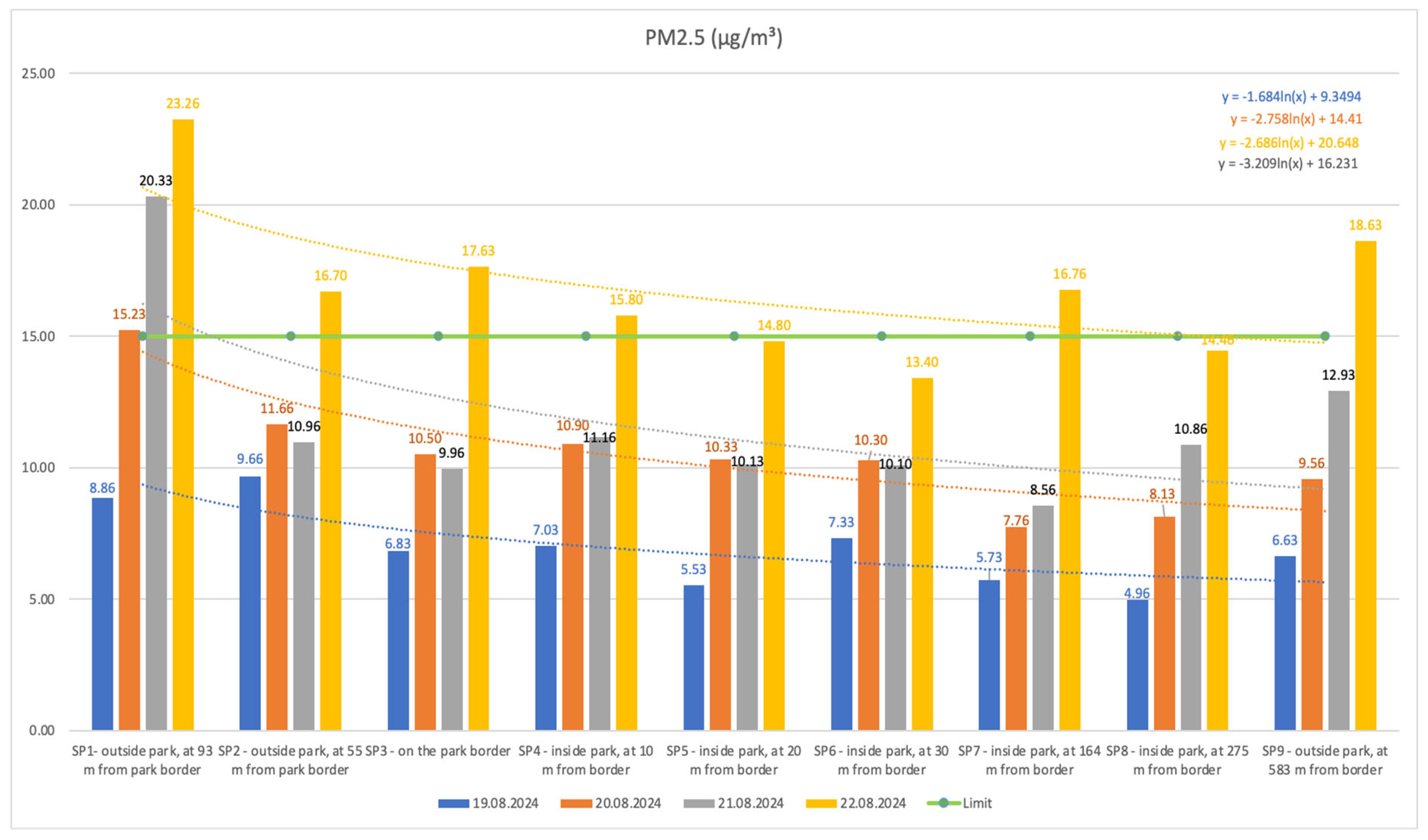
Figure 3.
Dynamics of air parameters by sample points (SP) and days (because of the large differences between values, HCHO and TVOC are not visible on the chart although are present in the chart center).
Figure 3.
Dynamics of air parameters by sample points (SP) and days (because of the large differences between values, HCHO and TVOC are not visible on the chart although are present in the chart center).
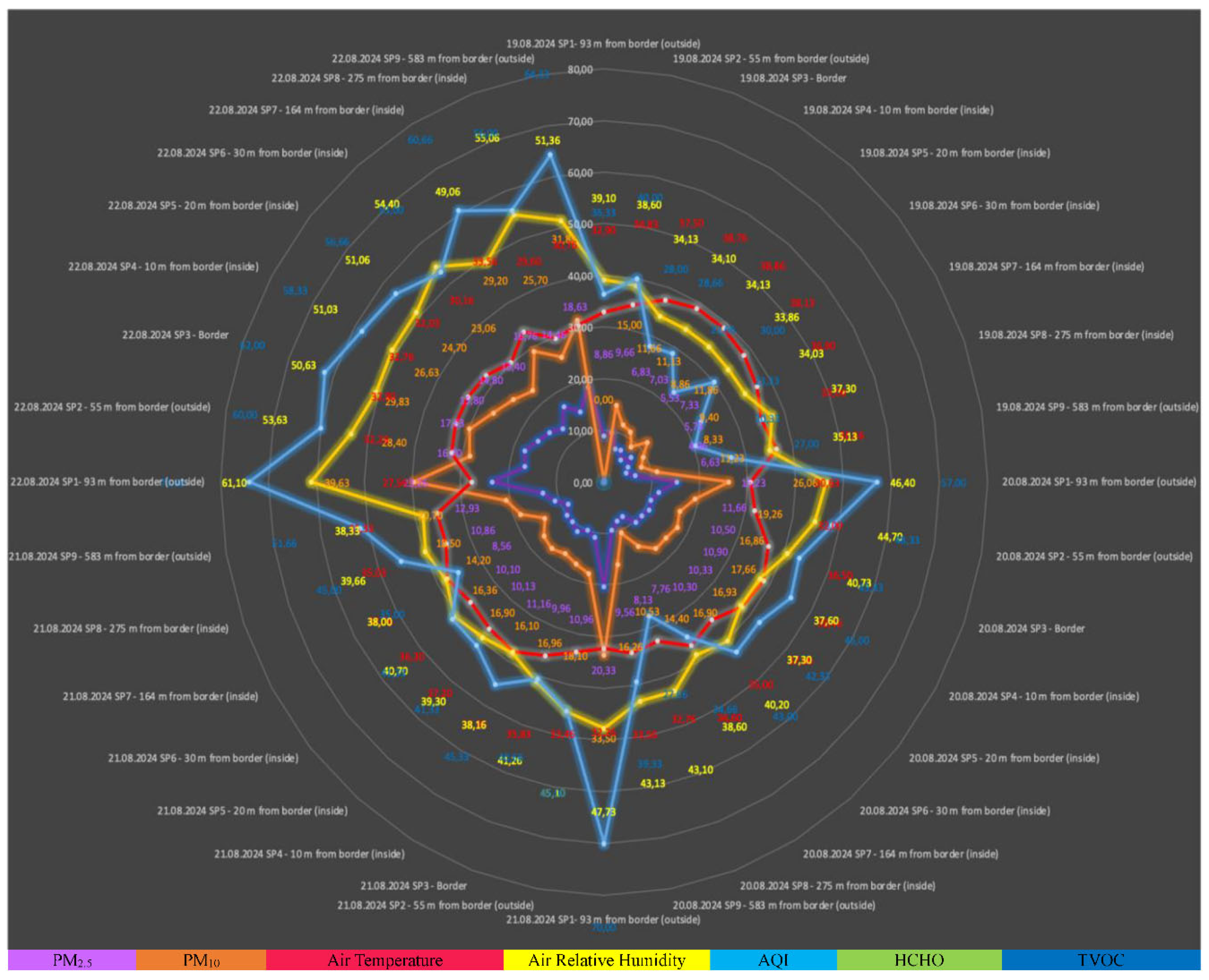
Figure 4.
Statistically significant correlations (Pearson correlations, p<0.05) between air quality parameters measured in the sample points (SP) – Day 1.
Figure 4.
Statistically significant correlations (Pearson correlations, p<0.05) between air quality parameters measured in the sample points (SP) – Day 1.
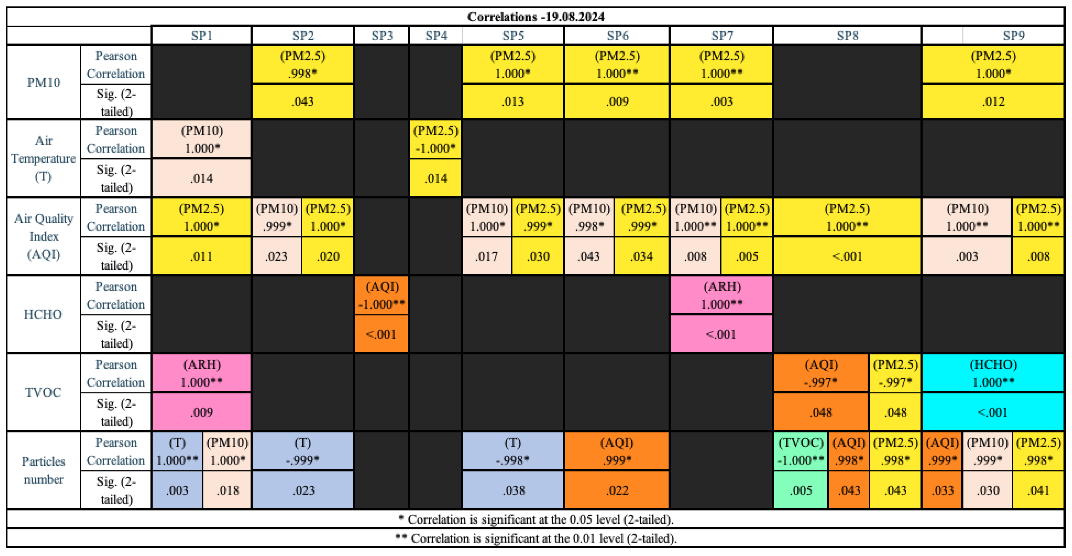
Figure 5.
Statistically significant correlations (Pearson correlations, p<0.05) between air quality parameters measured in the sample points (SP) – Day 2.
Figure 5.
Statistically significant correlations (Pearson correlations, p<0.05) between air quality parameters measured in the sample points (SP) – Day 2.
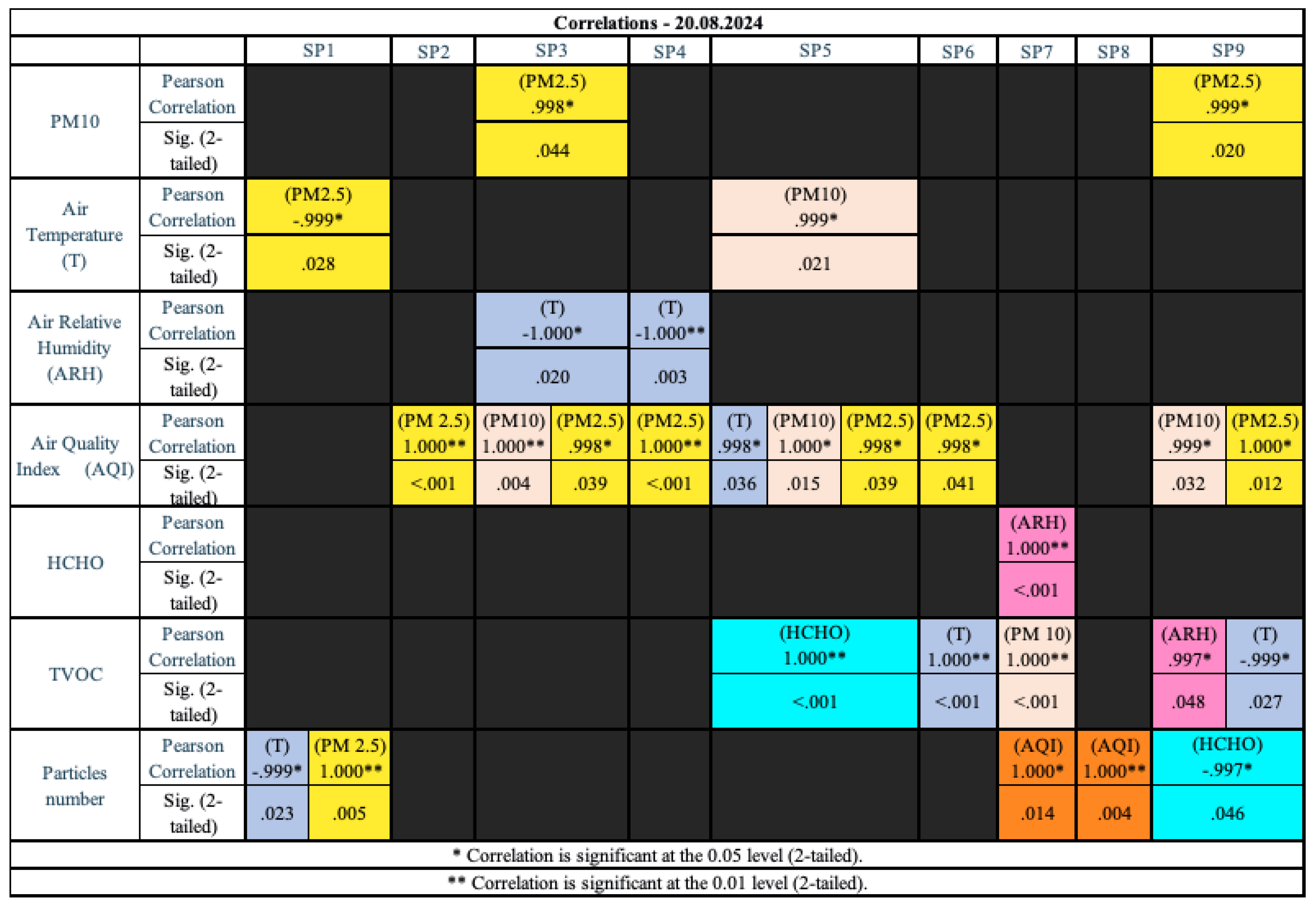
Figure 6.
Statistically significant correlations (Pearson correlations, p<0.05) between air quality parameters measured in the sample points (SP) – Day 3.
Figure 6.
Statistically significant correlations (Pearson correlations, p<0.05) between air quality parameters measured in the sample points (SP) – Day 3.
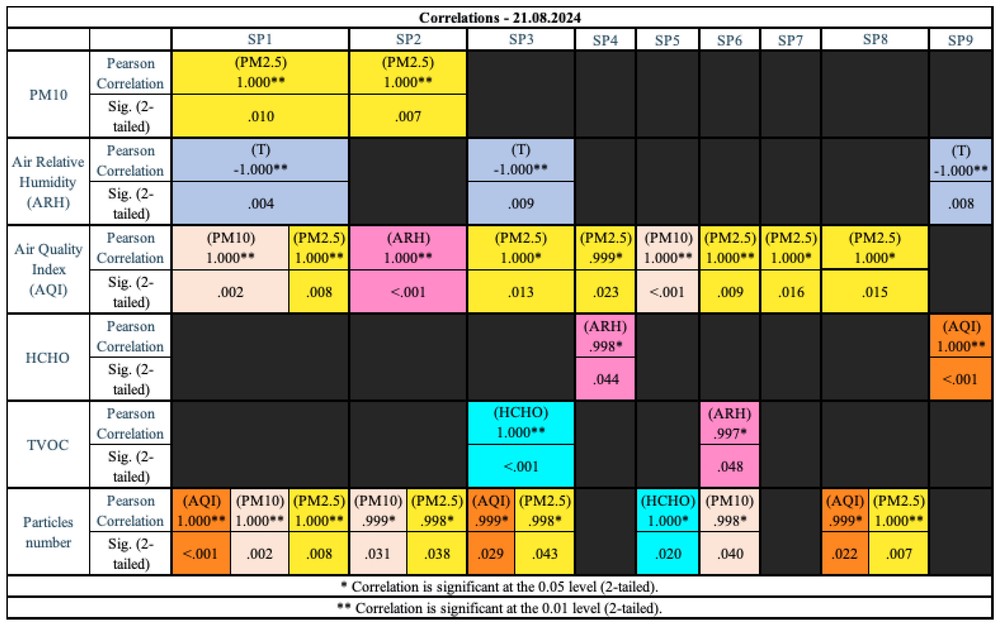
Figure 7.
Statistically significant correlations (Pearson correlations, p<0.05) between air quality parameters measured in the sample points (SP) – Day 4.
Figure 7.
Statistically significant correlations (Pearson correlations, p<0.05) between air quality parameters measured in the sample points (SP) – Day 4.
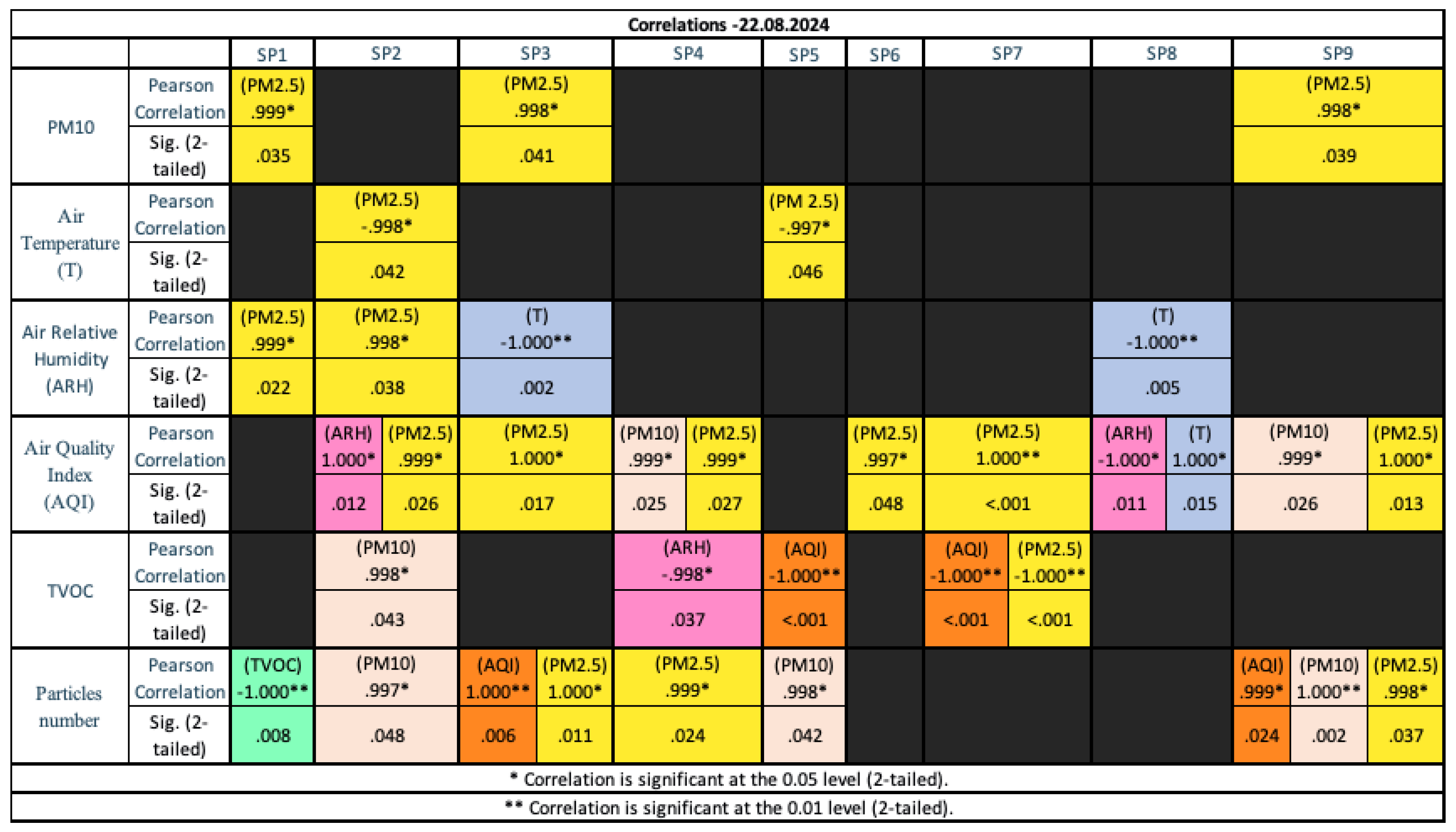
Figure 8.
Evolution of air PM10 concentrations (μg/m³) in the sample points (SP), within the analyzed period, related to daily (24 h) WHO recommended limit.
Figure 8.
Evolution of air PM10 concentrations (μg/m³) in the sample points (SP), within the analyzed period, related to daily (24 h) WHO recommended limit.
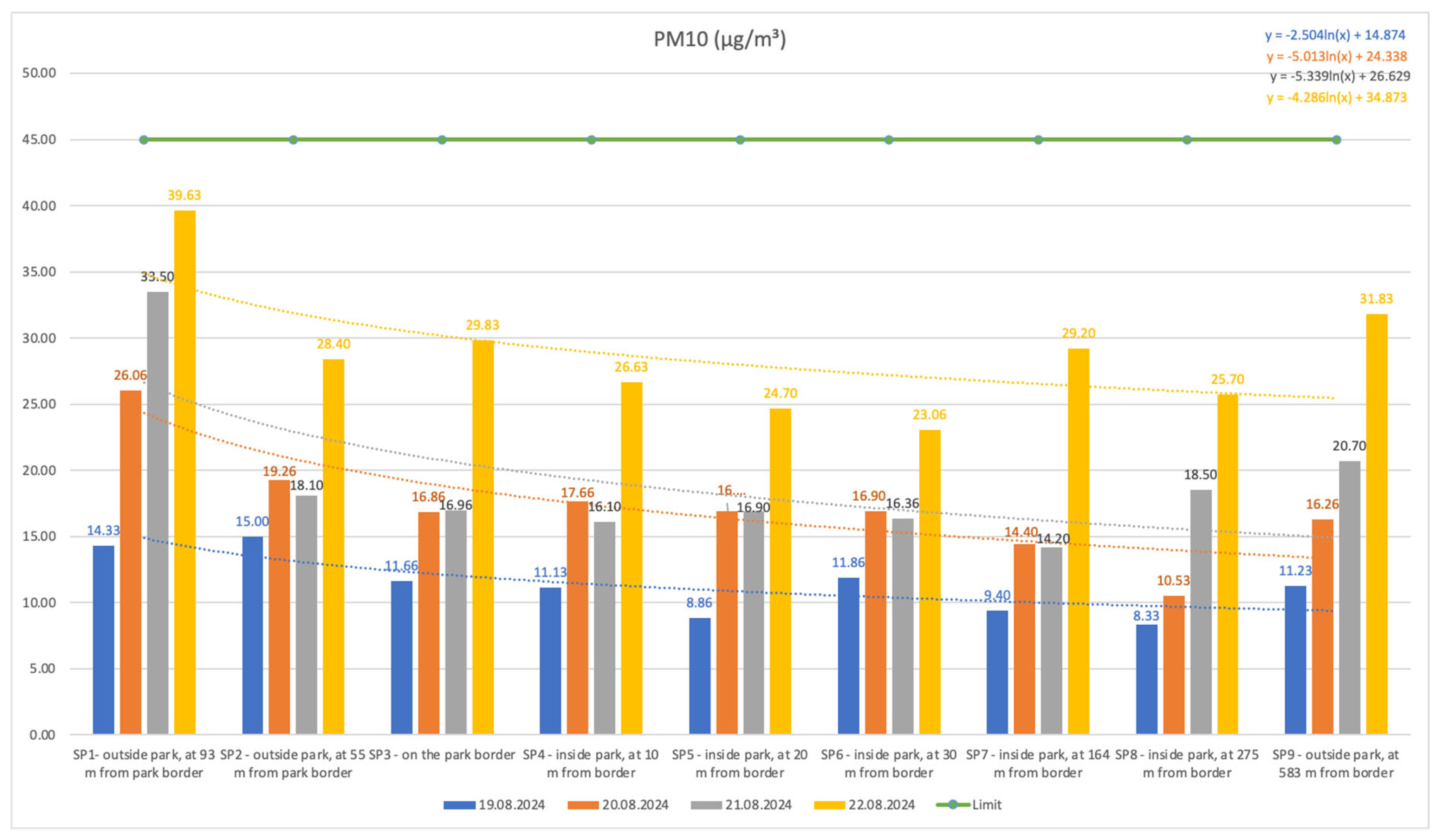
Figure 9.
Evolution of Air Quality Index (AQI) in the sample points (SP), within the analyzed period, related to United States Environmental Protection Agency (EPA) Standards (limits).
Figure 9.
Evolution of Air Quality Index (AQI) in the sample points (SP), within the analyzed period, related to United States Environmental Protection Agency (EPA) Standards (limits).
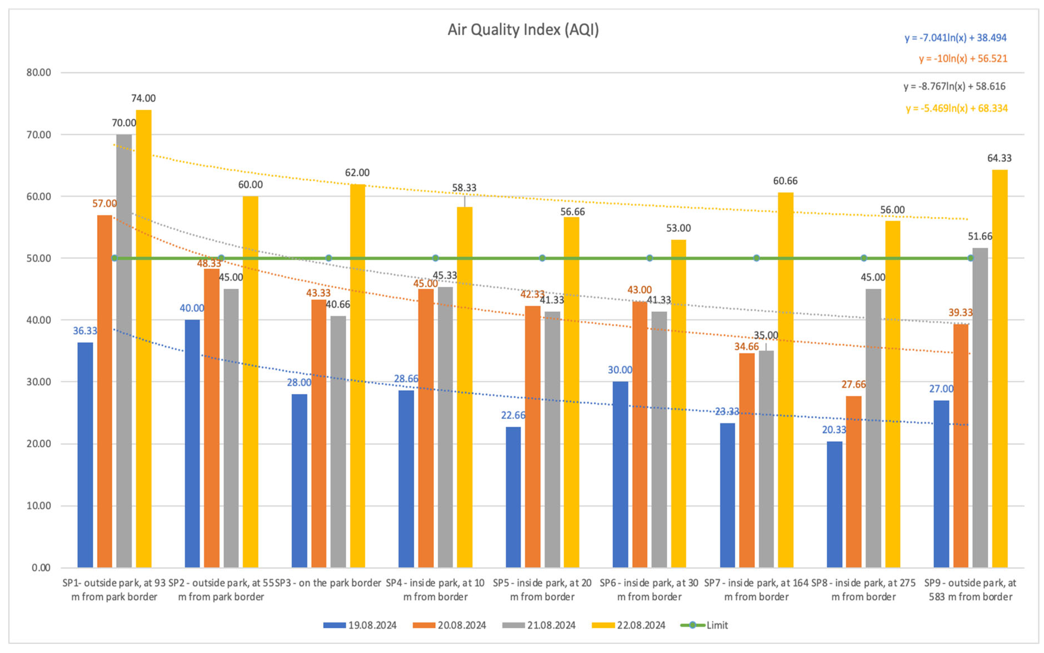
Figure 10.
Evolution of air particles number (amount, pcs/L) in the sample points (SP), within the analyzed period.
Figure 10.
Evolution of air particles number (amount, pcs/L) in the sample points (SP), within the analyzed period.
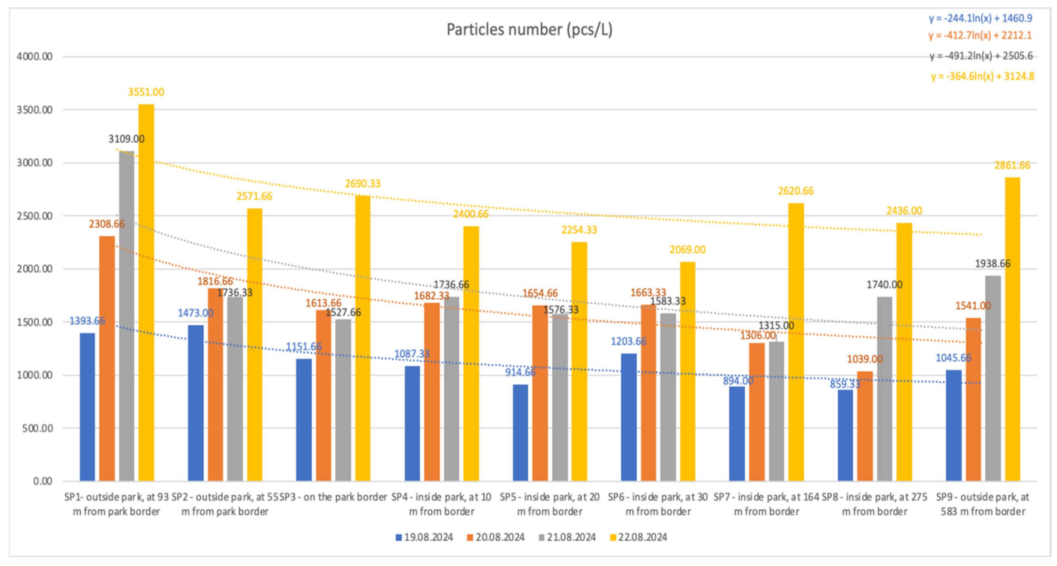
Figure 11.
Evolution of air temperature (°C) in the sample points (SP), within the analyzed period.
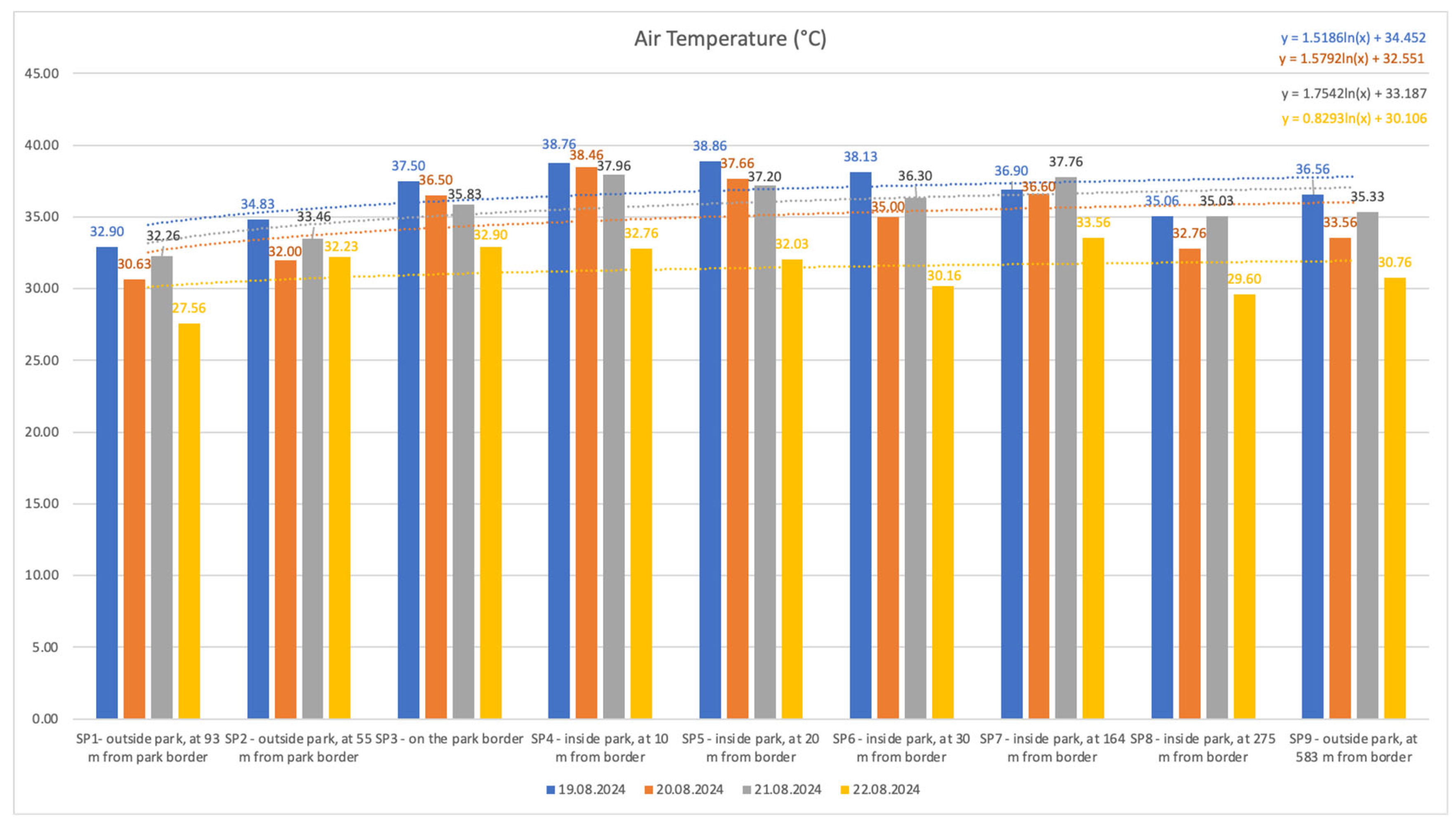
Figure 12.
Evolution of air relative humidity (%) in the sample points (SP), within the analyzed period.
Figure 12.
Evolution of air relative humidity (%) in the sample points (SP), within the analyzed period.
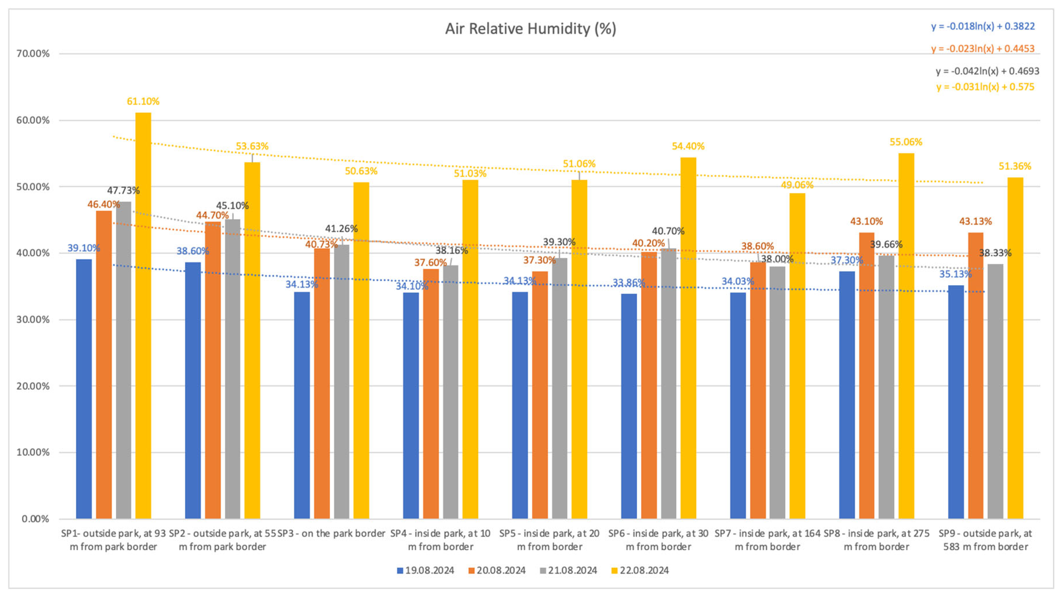
Figure 13.
Evolution of total volatile organic compounds (TVOC) concentrations (mg/m3) in the sample points (SP), within the analyzed period related to daily (24 h) WHO recommended limit.
Figure 13.
Evolution of total volatile organic compounds (TVOC) concentrations (mg/m3) in the sample points (SP), within the analyzed period related to daily (24 h) WHO recommended limit.
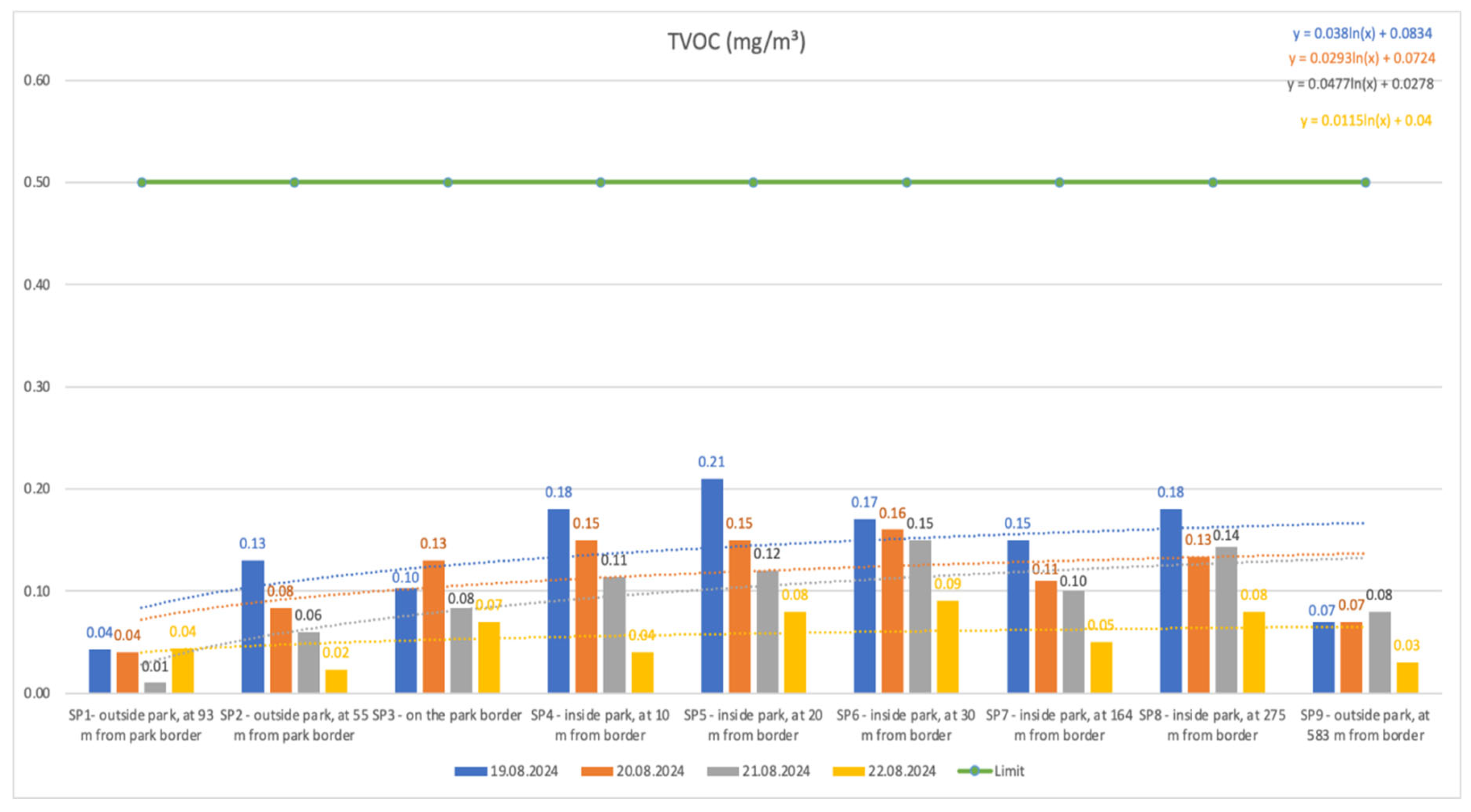
Figure 14.
Evolution of formaldehyde (HCHO) concentrations (mg/m3) in the sample points (SP), within the analyzed period related to daily (24 h) WHO recommended limit.
Figure 14.
Evolution of formaldehyde (HCHO) concentrations (mg/m3) in the sample points (SP), within the analyzed period related to daily (24 h) WHO recommended limit.
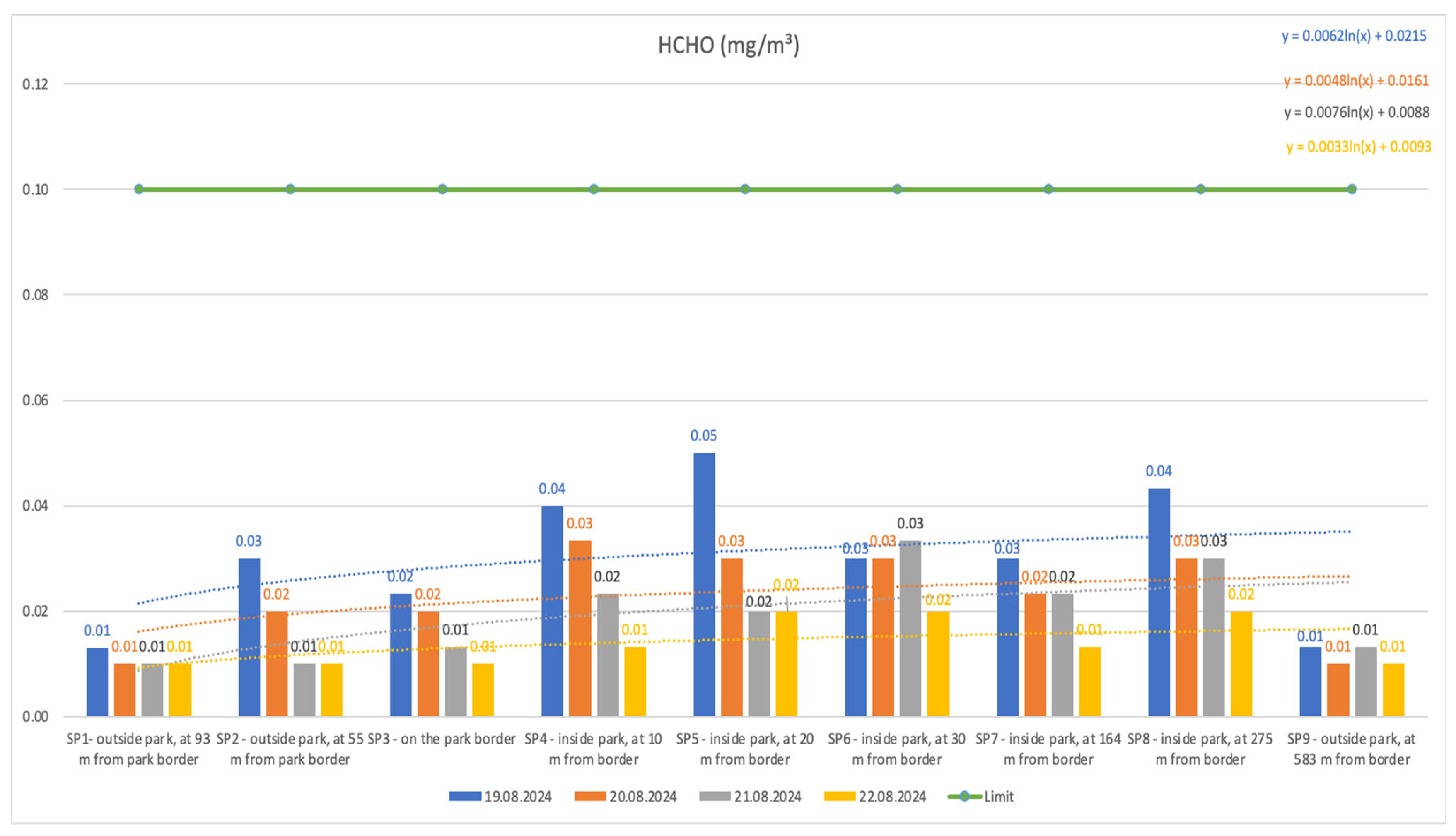

Table 1.
Measurement characteristics of the air quality monitor (measurement range and resolution) [26].
Table 1.
Measurement characteristics of the air quality monitor (measurement range and resolution) [26].
| Measurement characteristics | Air parameter | |||||
| PM2.5 | PM10 | HCHO | TVOC | Air Temperature | Air Relative Humidity | |
| Measurement range | 0 - 999 μg/m³ | 0 - 999 μg/m³ | 0 - 5 mg/m³ | 0 - 5 mg/m³ | 0-50°C | 0-90% |
| Measurement resolution | 0.1 μg/m³ | 0.1 μg/m³ | 0.01 mg/m³ | 0.01 mg/m³ | 0.01°C | 0.01% |
Table 2.
Reference levels and air quality ratings for the parameters PM2.5, PM10 and AQI (Air Quality Index).
Table 2.
Reference levels and air quality ratings for the parameters PM2.5, PM10 and AQI (Air Quality Index).
| Air quality parameter | |||||||||||
| PM2.5 (μg/m³) | PM10 (μg/m³) | AQI | |||||||||
| United States Environmental Protection Agency (EPA) Standards [26] | Air Quality Guidelines of World Health Organization [28] | Romanian Standard (Law no. 104/15 iunie 2011) [29] |
United States Environmental Protection Agency (EPA) Standards [26] | Air Quality Guidelines of World Health Organization [28] | Romanian Standard (Law no. 104/15 iunie 2011) [29] |
United States Environmental Protection Agency (EPA) Standards [26] | |||||
| PM2.5 Value (μg/m³) | Air quality level | PM2.5 Value (μg/m³) | 20 µg/m³ – Annual limit value for human health protection, which must be respected throughout the entire calendar year | PM10 Value (μg/m³) | Air quality level | PM10 Value (μg/m³) | PM10 Value (μg/m³) | AQI Value | Air quality level | ||
| ≤12 | Good | 5 (Annual) | 15 (24 h) | ≤54.9 | Good | 15 (Annual) | 45 (24 h) | 50 µg/m³ – Daily limit value for human health protection, which must not be exceeded more than 35 days a year 40 µg/m³ – Annual limit value for human health protection, this being the value that must be respected throughout the entire calendar year |
≤50 | Good | |
| 12.1 - 35.4 | Moderate | 55 – 154.9 | Moderate | 51 - 100 | Moderate | ||||||
| 35.5 - 55.4 | Unhealthy for Sensitive Groups | 155 – 254.9 | Unhealthy for Sensitive Groups | 101 - 150 | Unhealthy for Sensitive Groups | ||||||
| 55.5 - 150.4 | Unhealthy | 255 – 354.9 | Unhealthy | 151 - 200 | Unhealthy | ||||||
| 150.5 - 250.4 | Very Unhealthy | 355 – 424.9 | Very Unhealthy | 201 - 300 | Very Unhealthy | ||||||
| ≥ 250.5 | Hazardous | ≥425 | ≥301 | Hazardous | |||||||
Table 3.
Reference levels and air quality ratings for formaldehyde (HCHO) and TVOC concentrations [26,27].
| Air quality parameter | |||||||
| TVOC (mg/m³) | HCHO (mg/m³) | ||||||
| United States Environmental Protection Agency (EPA) Standards [26] | Air Quality Guidelines of World Health Organization [27] | Air Quality Guidelines of World Health Organization [27] | Romanian Standard (Law no. 104/15 iunie 2011; Directive 2004/107/CE) [29] |
||||
| TVOC Value (mg/m³) |
Air quality rating | TVOC Value (mg/m³) |
HCHO Value (mg/m³) |
HCHO Value (mg/m³) |
|||
| ≤0.5 | Healthy | Annual | 24 h | Annual | 24 h | 30 min. | ≤0.1 |
| - | ≤0.1 | ≤0.1 | |||||
| >0.5 | Unhealthy | - | 0.3-0.5 mg/m³ | - | >0.1 | >0.1 | |
Table 4.
Air quality parameters in the monitoring sample points, within the analyzed period.
| Monitoring date | Sample point (SP) | Air parameter | |||||||
| PM2.5 (μg/m³) | PM10 (μg/m³) | Air Temperature (°C) | Air Relative Humidity (%) | AQI | HCHO (mg/m³) |
TVOC (mg/m³) |
Number of particles | ||
| Day 1 | SP1 – outside park, at 93 m from park border | 8.86 ±3.23 |
14.33 ±4.80 |
32.90 ±0.26 |
39.10 ±0.43 |
36.33 ±12.74 |
0.013 ±0.005 |
0.04 ±0.04 |
1393.66 ±453.18 |
| SP2 – outside park, at 55 m from park border | 9.66 ±2.71 |
15.00 ±4.50 |
34.83 ±0.50 |
38.60 ±0.40 |
40.00 ±11.53 |
0.03 ±0.010 |
0.13 ±0.03 |
1473.00 ±359.63 |
|
| SP3 – on the park border | 6.83 ±0.49 |
11.66 ±0.58 |
37.50 ±0.62 |
34.13 ±0.51 |
28.00 ±1.73 |
0.02 ±0.01 |
0.10 ±0.04 |
1151.66 ±102.92 |
|
| SP4 – inside park, at 10 m from border | 7.03 ±0.86 |
11.13 ±0.46 |
38.76 ±0.30 |
34.10 ±0.10 |
28.66 ±3.51 |
0.04 ±0.00 |
0.18 ±0.00 |
1087.33 ±122.83 |
|
| SP5 – inside park, at 20 m from border | 5.53 ±0.40 |
8.86 ±0.70 |
38.86 ±0.11 |
34.13 ±0.55 |
22.66 ±1.52 |
0.05 ±0.00 |
0.21 ±0.01 |
914.66 ±8.38 |
|
| SP6 – inside park, at 30 m from border | 7.33 ±1.05 |
11.86 ±1.66 |
38.13 ±0.15 |
33.86 ±0.95 |
30.00 ±4.58 |
0.03 ±0.005 |
0.17 ±0.02 |
1203.66 ±172.81 |
|
| SP 7 – inside park, at 164 m from border | 5.73 ±0.96 |
9.40 ±1.67 |
36.90 ±0.10 |
34.03 ±0.05 |
23.33 ±4.04 |
0.03 ±0.01 |
0.15 ±0.03 |
894.00 ±164.83 |
|
| SP8 – inside park, at 275 m from border | 4.96 ±0.50 |
8.33 ±1.45 |
35.06 ±0.20 |
37.30 ±0.70 |
20.33 ±2.51 |
0.04 ±0.005 |
0.18 ±0.01 |
859.33 ±116.42 |
|
| SP9 – outside park, at 583 m from border | 6.63 ±1.96 |
11.23 ±3.61 |
36.56 ±0.92 |
35.13 ±1.68 |
27.00 ±7.81 |
0.01 ±0.005 |
0.07 ±0.01 |
1045.66 ±281.03 |
|
| Day 2 | SP1 – outside park, at 93 m from park border | 15.23 ±1.82 |
26.06 ±3.18 |
30.63 ±0.50 |
46.40 ±0.30 |
57.00 ±3.60 |
0.01 ±0.00 |
0.04 ±0.01 |
2308.66 ±273.63 |
| SP2 – outside park, at 55 m from park border | 11.66 ±0.50 |
19.26 ±1.02 |
32.00 ±0.20 |
44.70 ±0.45 |
48.33 ±2.51 |
0.02 ±0.00 |
0.08 ±0.01 |
1816.66 ±101.63 |
|
| SP3 – on the park border | 10.50 ±1.70 |
16.86 ±1.87 |
36.50 ±1.17 |
40.73 ±1.49 |
43.33 ±7.09 |
0.02 ±0.005 |
0.13 ±0.00 |
1613.66 ±262.8 |
|
| SP4 – inside park, at 10 m from border | 10.90 ±0.90 |
17.66 ±1.70 |
38.46 ±0.60 |
37.60 ±0.95 |
45.00 ±4.00 |
0.03 ±0.005 |
0.15 ±0.01 |
1682.33 ±174.61 |
|
| SP5 – inside park, at 20 m from border | 10.33 ±1.61 |
16.93 ±2.45 |
37.66 ±1.15 |
37.30 ±0.79 |
42.33 ±7.02 |
0.03 ±0.005 |
0.15 ±0.01 |
1654.66 ±204.39 |
|
| SP6 – inside park, at 30 m from border | 10.30 ±0.78 |
16.90 ±0.72 |
35.00 ±0.30 |
40.20 ±0.78 |
43.00 ±1.73 |
0.03 ±0.005 |
0.16 ±0.02 |
1663.33 ±105.64 |
|
| SP 7 – inside park, at 164 m from border | 7.76 ±1.90 |
14.40 ±1.30 |
36.60 ±1.27 |
38.60 ±1.90 |
34.66 ±3.78 |
0.02 ±0.005 |
0.11 ±0.01 |
1306.00 ±110.43 |
|
| SP8 – inside park, at 275 m from border | 8.13 ±1.15 |
10.53 ±1.89 |
32.76 ±0.35 |
43.10 ±0.70 |
27.66 ±6.11 |
0.03 ±0.00 |
0.13 ±0.01 |
1039.00 ±208.51 |
|
| SP9 – outside park, at 583 m from border | 9.56 ±1.20 |
16.26 ±1.80 |
33.56 ±0.80 |
43.13 ±1.68 |
39.33 ±5.03 |
0.01 ±0.005 |
0.07 ±0.02 |
1541.00 ±125.03 |
|
| Day 3 | SP1 – outside park, at 93 m from park border | 20.33 ±8.05 |
33.50 ±14.70 |
32.26 ±2.02 |
47.73 ±3.69 |
70.00 ±19.97 |
0.01 ±0.00 |
0.01 ±0.01 |
3109.00 ±1229.73 |
| SP2 – outside park, at 55 m from park border | 10.96 ±1.00 |
18.10 ±2.06 |
33.46 ±0.25 |
45.10 ±0.80 |
45.00 ±4.00 |
0.01 ±0.00 |
0.06 ±0.01 |
1736.33 ±172.63 |
|
| SP3 – on the park border | 9.96 ±0.85 |
16.96 ±2.05 |
35.83 ±1.32 |
41.26 ±3.05 |
40.66 ±3.21 |
0.01 ±0.005 |
0.08 ±0.02 |
1527.66 ±173.09 |
|
| SP4 – inside park, at 10 m from border | 11.16 ±1.95 |
16.10 ±4,58 |
37.96 ±0.15 |
38.16 ±0.72 |
45.33 ±7.50 |
0.02 ±0.005 |
0.11 ±0.01 |
1736.66 ±305.78 |
|
| SP5 – inside park, at 20 m from border | 10.13 ±0.15 |
16.90 ±0.34 |
37.20 ±0.17 |
39.30 ±0.10 |
41.33 ±0,57 |
0.02 ±0.005 |
0.12 ±0.01 |
1576.33 ±48.8 |
|
| SP6 – inside park, at 30 m from border | 10.10 ±0.98 |
16.36 ±1.75 |
36.30 ±0.90 |
40.70 ±1.15 |
41.33 ±4.16 |
0.03 ±0.005 |
0.15 ±0.01 |
1583.33 ±163.72 |
|
| SP 7 – inside park, at 164 m from border | 8.56 ±1.07 |
14.20 ±1.60 |
37.76 ±2.10 |
38.00 ±2.23 |
35.00 ±4.35 |
0.02 ±0.00 |
0.10 ±0.01 |
1315.00 ±186.67 |
|
| SP8 – inside park, at 275 m from border | 10.86 ±1.42 |
18.50 ±2.26 |
35.03 ±1.05 |
39.66 ±0.66 |
45.00 ±6.08 |
0.03 ±0.00 |
0.14 ±0.01 |
1740.00 ±218.86 |
|
| SP9 – outside park, at 583 m from border | 12.93 ±0.55 |
20.70 ±1.37 |
35.33 ±2.01 |
38.33 ±2.81 |
51.66 ±1.15 |
0.01 ±0.005 |
0.08 ±0.01 |
1938.66 ±80.32 |
|
| Day 4 | SP1 – outside park, at 93 m from park border | 23.26 ±0.32 |
39.63 ±0.98 |
27.56 ±0.15 |
61.10 ±0.26 |
74.00 ±1.00 |
0.01 ±0.00 |
0.04 ±0.01 |
3551.00 ±47.46 |
| SP2 – outside park, at 55 m from park border | 16.70 ±1.73 |
28.40 ±3.73 |
32.23 ±1.71 |
53.63 ±3.46 |
60.00 ±3.60 |
0.01 ±0.00 |
0.02 ±0.01 |
2571.66 ±278.5 |
|
| SP3 – on the park border | 17.63 ±4.25 |
29.83 ±7.57 |
32.90 ±1.76 |
50.63 ±1.92 |
62.00 ±8.71 |
0.01 ±0.005 |
0.07 ±0.01 |
2690.33 ±597.53 |
|
| SP4 – inside park, at 10 m from border | 15.80 ±2.83 |
26.63 ±4.16 |
32.76 ±0.90 |
51.03 ±1.00 |
58.33 ±5.85 |
0.01 ±0.005 |
0.04 ±0.01 |
2400.66 ±433.96 |
|
| SP5 – inside park, at 20 m from border | 14.80 ±0.30 |
24.70 ±1.68 |
32.03 ±0.80 |
51.06 ±1.32 |
56.66 ±0.57 |
0.02 ±0.00 |
0.08 ±0.01 |
2254.33 ±122.78 |
|
| SP6 – inside park, at 30 m from border | 13.40 ±1.15 |
23.06 ±1.97 |
30.16 ±0.30 |
54.40 ±0.52 |
53.00 ±2.00 |
0.02 ±0.00 |
0.09 ±0.01 |
2069.00 ±173.51 |
|
| SP 7 – inside park, at 164 m from border | 16.76 ±0.05 |
29.20 ±0.52 |
33.56 ±1.04 |
49.06 ±1.68 |
60.66 ±0.57 |
0.01 ±0.005 |
0.05 ±0.01 |
2620.66 ±26.63 |
|
| SP8 – inside park, at 275 m from border | 14.46 ±3.02 |
25.70 ±5.12 |
29.60 ±1.15 |
55.06 ±2.45 |
56.00 ±6.24 |
0.02 ±0.00 |
0.08 ±0.01 |
2436.00 ±484.90 |
|
| SP9 – outside park, at 583 m from border | 18.63 ±5.29 |
31.83 ±8.94 |
30.76 ±1.41 |
51.36 ±3.35 |
64.33 ±11.37 |
0.01 ±0.00 |
0.03 ±0.02 |
2861.66 ±794.31 |
|
Table 5.
Statistical significant differences (Paired-samples t-test, p<0.05) between sample points (SP) regarding the values of the measured air parameters, within the analyzed period.
Table 5.
Statistical significant differences (Paired-samples t-test, p<0.05) between sample points (SP) regarding the values of the measured air parameters, within the analyzed period.
| Crt. No. | Statistically significant differences (Paired-samples t-test, p<0.05) regarding the air quality parameters between sample points (SP) – Day 1 | |||||||
| Air parameter | ||||||||
| PM2.5 | PM10 | AQI | Particles number | Air Relative Humidity | Air Temperature | TVOC | HCHO | |
| 1 | SP2 - SP7 | SP2 - SP7 | SP2 - SP7 | SP2 - SP4 | SP1 - SP2 | SP1 - SP2 | SP1 - SP2 | SP1 - SP4 |
| 2 | SP2 - SP8 | SP3 - SP5 | SP2 - SP8 | SP3 - SP5 | SP1 - SP3 | SP1 - SP3 | SP1 - SP4 | SP1 - SP5 |
| 3 | SP3 - SP5 | SP3 - SP8 | SP3 - SP5 | SP5 - SP6 | SP1 - SP4 | SP1 - SP4 | SP1 - SP5 | SP1 - SP6 |
| 4 | SP3 - SP8 | SP4 - SP5 | SP3 - SP8 | - | SP1 - SP5 | SP1 - SP5 | SP1 - SP6 | SP1 - SP7 |
| 5 | SP4 - SP7 | SP4 - SP8 | SP4 - SP7 | - | SP1 - SP6 | SP1 - SP6 | SP1 - SP7 | SP2 - SP5 |
| 6 | SP4 - SP8 | SP5 - SP6 | SP4 - SP8 | - | SP1 - SP7 | SP1 - SP7 | SP1 - SP8 | SP2 - SP9 |
| 7 | SP5 - SP6 | - | SP5 - SP6 | - | SP1 - SP8 | SP1 - SP8 | SP2 - SP5 | SP3 - SP5 |
| 8 | SP6 - SP8 | - | - | - | SP1 - SP9 | SP1 - SP9 | SP2- SP8 | SP3 - SP6 |
| 9 | - | - | - | - | SP2 - SP3 | SP2 - SP3 | SP2 - SP9 | SP4 - SP9 |
| 10 | - | - | - | - | SP2 - SP4 | SP2 - SP4 | SP3 - SP4 | SP5 - SP6 |
| 11 | - | - | - | - | SP2 - SP5 | SP2 - SP5 | SP3 - SP5 | SP5 - SP9 |
| 12 | - | - | - | - | SP2 - SP6 | SP2 - SP6 | SP3 - SP6 | SP6 - SP9 |
| 13 | - | - | - | - | SP2 - SP7 | SP2 - SP7 | SP4 - SP5 | SP7 - SP9 |
| 14 | - | - | - | - | SP2 - SP8 | SP2 - SP9 | SP4 - SP9 | SP8 - SP9 |
| 15 | - | - | - | - | SP2 - SP9 | SP3 - SP4 | SP5 - SP6 | - |
| 16 | - | - | - | - | SP3 - SP8 | SP3 - SP5 | SP5 - SP9 | - |
| 17 | - | - | - | - | SP4 - SP8 | SP3 - SP8 | SP6 - SP9 | - |
| 18 | - | - | - | - | SP5 - SP8 | SP3 - SP9 | SP7 - SP9 | - |
| 19 | - | - | - | - | SP6 - SP8 | SP4 - SP7 | SP8 - SP9 | - |
| 20 | - | - | - | - | SP6 - SP9 | SP4 - SP8 | - | - |
| 21 | - | - | - | - | SP7 - SP8 | SP4 - SP9 | - | - |
| 22 | - | - | - | - | - | SP5 - SP6 | - | - |
| 23 | - | - | - | - | - | SP5 - SP7 | - | - |
| 24 | - | - | - | - | - | SP5 - SP8 | - | - |
| 25 | - | - | - | - | - | SP5 - SP9 | - | - |
| 26 | - | - | - | - | - | SP6 - SP7 | - | - |
| 27 | - | - | - | - | - | SP6 - SP8 | - | - |
| 28 | - | - | - | - | - | SP7 - SP8 | - | - |
| No. | Statistically significant differences (Paired-samples t-test, p<0.05) regarding the air quality parameters between sample points (SP) – Day 2 | |||||||
| Air parameter | ||||||||
| PM2.5 | PM10 | AQI | Particles number | Air Relative Humidity | Air Temperature | TVOC | HCHO | |
| 1 | SP1 - SP2 | SP1 - SP2 | SP1 - SP2 | SP1 - SP2 | SP1 - SP2 | SP1 - SP2 | SP1 - SP2 | SP1 - SP3 |
| 2 | SP1 - SP3 | SP1 - SP3 | SP1 - SP3 | SP1 - SP3 | SP1 - SP3 | SP1 - SP3 | SP1 - SP3 | SP1 - SP4 |
| 3 | SP1 - SP4 | SP1 - SP4 | SP1 - SP4 | SP1 - SP4 | SP1 - SP4 | SP1 - SP4 | SP1 - SP4 | SP1 - SP5 |
| 4 | SP1- SP5 | SP1 - SP5 | SP1 - SP5 | SP1 - SP5 | SP1 - SP5 | SP1 - SP5 | SP1 - SP5 | SP1 - SP6 |
| 5 | SP1 - SP6 | SP1 - SP6 | SP1 - SP6 | SP1 - SP6 | SP1 - SP6 | SP1 - SP6 | SP1 - SP6 | SP1 - SP7 |
| 6 | SP1 - SP7 | SP1 - SP7 | SP1 - SP7 | SP1 - SP7 | SP1 - SP7 | SP1 - SP7 | SP1 - SP7 | SP2 - SP4 |
| 7 | SP1 - SP8 | SP1 - SP8 | SP1 - SP8 | SP1 - SP8 | SP1 - SP8 | SP1 - SP8 | SP1 - SP8 | SP2 - SP5 |
| 8 | SP1 - SP9 | SP1 - SP9 | SP1 - SP9 | SP1 - SP9 | SP1 - SP9 | SP1 - SP9 | SP2 - SP3 | SP2 - SP6 |
| 9 | SP2 - SP7 | SP2 - SP3 | SP2 - SP7 | SP2 - SP7 | SP2 - SP3 | SP2 - SP3 | SP2 - SP4 | SP4 - SP9 |
| 10 | SP2 - SP8 | SP2 - SP6 | SP2 - SP8 | SP2 - SP8 | SP2 - SP4 | SP2 - SP4 | SP2 - SP5 | SP5 - SP7 |
| 11 | SP4 - SP7 | SP2 - SP7 | SP3 - SP8 | SP3 - SP8 | SP2 - SP5 | SP2 - SP5 | SP2 - SP6 | SP5 - SP9 |
| 12 | SP4 - SP8 | SP2 - SP8 | SP4 - SP7 | SP4 - SP7 | SP2 - SP6 | SP2 - SP6 | SP2 - SP7 | SP6 - SP7 |
| 13 | SP5 - SP8 | SP3 - SP8 | SP4 - SP8 | SP4 - SP8 | SP2 - SP7 | SP2 - SP7 | SP2 - SP8 | SP8 - SP9 |
| 14 | SP6 - SP7 | SP4 - SP7 | SP5 - SP7 | SP5 - SP7 | SP2 - SP8 | SP2 - SP9 | SP3 - SP4 | - |
| 15 | SP6 - SP8 | SP4 - SP8 | SP6- SP7 | SP5 - SP8 | SP3 - SP4 | SP3 - SP4 | SP3 - SP7 | - |
| 16 | - | SP5 - SP7 | SP6 - SP8 | SP6 - SP7 | SP3 - SP5 | SP3 - SP8 | SP3 - SP9 | - |
| 17 | - | SP5 - SP8 | - | SP6 - SP8 | SP3 - SP7 | SP3 - SP9 | SP4 - SP7 | - |
| 18 | - | SP6 - SP7 | - | SP8 - SP9 | SP3 - SP9 | SP4 - SP6 | SP4 - SP9 | - |
| 19 | - | SP6 - SP8 | - | - | SP4 - SP6 | SP4 - SP7 | SP5 - SP7 | - |
| 20 | - | SP8 - SP9 | - | - | SP4 - SP8 | SP4 - SP8 | SP5 - SP9 | - |
| 21 | - | - | - | - | SP4 - SP9 | SP4 - SP9 | SP6 - SP7 | - |
| 22 | - | - | - | - | SP5 - SP6 | SP5 - SP6 | SP6 - SP8 | - |
| 23 | - | - | - | - | SP5 - SP8 | SP5 - SP8 | SP6 - SP9 | - |
| 24 | - | - | - | - | SP5 - SP9 | SP5 - SP9 | SP7 - SP8 | - |
| 25 | - | - | - | - | SP6 - SP8 | SP6 - SP8 | SP7 - SP9 | - |
| 26 | - | - | - | - | SP7 - SP8 | SP7 - SP8 | SP8 - SP9 | - |
| 27 | - | - | - | - | SP7 - SP9 | SP7 - SP9 | - | - |
| No. | Statistically significant differences (Paired-samples t-test, p<0.05) regarding the air quality parameters between sample points (SP) – Day 3 | |||||||
| Air parameter | ||||||||
| PM2.5 | PM10 | AQI | Particles number | Air Relative Humidity | Air Temperature | TVOC | HCHO | |
| 1 | SP2 - SP3 | SP1 - SP4 | SP1 - SP4 | SP2 - SP3 | SP1- SP3 | SP1 - SP3 | SP1 - SP2 | SP1- SP4 |
| 2 | SP2 - SP7 | SP2 - SP7 | SP1 - SP6 | SP2 - SP7 | SP1- SP4 | SP1 - SP4 | SP1 - SP3 | SP1 - SP5 |
| 3 | SP2 - SP9 | SP3 - SP7 | SP1 - SP8 | SP3 - SP9 | SP1 - SP5 | SP1 - SP5 | SP1 - SP4 | SP1 - SP6 |
| 4 | SP3 - SP9 | SP3 - SP9 | SP2- SP3 | SP5 - SP9 | SP1 - SP6 | SP1 - SP7 | SP1 - SP5 | SP1 - SP7 |
| 5 | SP5 - SP9 | SP5 - SP7 | SP2 - SP7 | SP6 - SP9 | SP1- SP7 | SP1 - SP9 | SP1 - SP6 | SP2 - SP4 |
| 6 | SP6 - SP9 | SP5 - SP9 | SP2 - SP9 | SP7 - SP9 | SP1 - SP8 | SP2 - SP3 | SP1 - SP7 | SP2 - SP5 |
| 7 | SP7 - SP9 | SP6 - SP8 | SP3 - SP9 | - | SP1 - SP9 | SP2 - SP4 | SP1 - SP8 | SP2 - SP6 |
| 8 | SP8 - SP9 | SP6 - SP9 | SP5 - SP9 | - | SP2 - SP3 | SP2 - SP5 | SP1 - SP9 | SP2 - SP7 |
| 9 | - | SP7 - SP8 | SP6 - SP9 | - | SP2 - SP4 | SP2 - SP6 | SP2 - SP4 | SP3 - SP6 |
| 10 | - | SP7 - SP9 | SP7 - SP9 | - | SP2 - SP5 | SP2 - SP7 | SP2 - SP5 | SP3 - SP8 |
| 11 | - | - | - | - | SP2 - SP6 | SP3 - SP7 | SP2- SP6 | SP6 - SP9 |
| 12 | - | - | - | - | SP2 - SP7 | SP4 - SP5 | SP2 - SP7 | SP8 - SP9 |
| 13 | - | - | - | - | SP2 - SP8 | SP4 - SP6 | SP2- SP8 | - |
| 14 | - | - | - | - | SP2 - SP9 | SP4 - SP8 | SP3 - SP6 | - |
| 15 | - | - | - | - | SP3 - SP7 | SP5 - SP8 | SP3- SP8 | - |
| 16 | - | - | - | - | SP3 - SP9 | SP6 - SP8 | SP4 - SP6 | - |
| 17 | - | - | - | - | SP4 - SP5 | SP7 - SP9 | SP4 - SP8 | - |
| 18 | - | - | - | - | SP4 - SP6 | - | SP4 - SP9 | - |
| 19 | - | - | - | - | SP4 - SP8 | - | SP5 - SP9 | - |
| 20 | - | - | - | - | - | - | SP6 - SP7 | - |
| 21 | - | - | - | - | - | - | SP6 - SP9 | - |
| 22 | - | - | - | - | - | - | SP7 - SP8 | - |
| 23 | - | - | - | - | - | - | SP8 - SP9 | - |
| No. | Statistically significant differences (Paired-samples t-test, p<0.05) regarding the air quality parameters between sample points (SP) – Day 4 | |||||||
| Air parameter | ||||||||
| PM2.5 | PM10 | AQI | Particles number | Air Relative Humidity | Air Temperature | TVOC | HCHO | |
| 1 | SP1 - SP2 | SP1 - SP2 | SP1 - SP2 | SP1 - SP2 | SP1 - SP2 | SP1 - SP2 | SP1 - SP5 | - |
| 2 | SP1 - SP4 | SP1 - SP4 | SP1 - SP4 | SP1 - SP4 | SP1 - SP3 | SP1 - SP3 | SP1 - SP6 | - |
| 3 | SP1 - SP5 | SP1 - SP5 | SP1 - SP5 | SP1 - SP5 | SP1 - SP4 | SP1 - SP4 | SP1 - SP8 | - |
| 4 | SP1 - SP6 | SP1 - SP6 | SP1 - SP6 | SP1 - SP6 | SP1 - SP5 | SP1 - SP5 | SP2 - SP3 | - |
| 5 | SP1 - SP7 | SP1 - SP7 | SP1 - SP7 | SP1 - SP7 | SP1 - SP6 | SP1 - SP6 | SP2 - SP5 | - |
| 6 | SP1 - SP8 | SP1 - SP8 | SP1 - SP8 | SP1 - SP8 | SP1 - SP7 | SP1 - SP7 | SP2 - SP6 | - |
| 7 | SP2 - SP6 | SP2 - SP4 | SP2 - SP6 | SP2 - SP6 | SP1 - SP8 | SP1 - SP8 | SP2 - SP7 | - |
| 8 | SP5 - SP7 | SP2 - SP6 | SP3 - SP8 | SP5 - SP6 | SP1 - SP9 | SP1 - SP9 | SP2 - SP8 | - |
| 9 | SP6 - SP7 | SP4 - SP6 | SP5 - SP6 | SP5 - SP7 | SP2 - SP7 | SP2 - SP7 | SP3 - SP4 | - |
| 10 | - | SP5 - SP7 | SP5 - SP7 | SP6 - SP7 | SP2 - SP9 | SP2 - SP9 | SP3 - SP7 | - |
| 11 | - | SP6 - SP7 | SP6 - SP7 | - | SP3 - SP6 | SP4 - SP6 | SP4 - SP5 | - |
| 12 | - | - | - | - | SP3 - SP8 | SP4 - SP8 | SP4 - SP6 | - |
| 13 | - | - | - | - | SP4 - SP6 | SP4 - SP9 | SP4 - SP7 | - |
| 14 | - | - | - | - | SP4 - SP7 | SP5 - SP6 | SP4- SP8 | - |
| 15 | - | - | - | - | SP5 - SP6 | SP5 - SP8 | SP6 - SP7 | - |
| 16 | - | - | - | - | SP5 - SP8 | SP6 - SP7 | SP6 - SP9 | - |
| 17 | - | - | - | - | SP6 - SP7 | SP7 - SP8 | SP7 - SP8 | - |
| 18 | - | - | - | - | - | SP7 - SP9 | SP8 - SP9 | - |
| 19 | - | - | - | - | - | SP8 - SP3 | - | - |
Disclaimer/Publisher’s Note: The statements, opinions and data contained in all publications are solely those of the individual author(s) and contributor(s) and not of MDPI and/or the editor(s). MDPI and/or the editor(s) disclaim responsibility for any injury to people or property resulting from any ideas, methods, instructions or products referred to in the content. |
© 2025 by the authors. Licensee MDPI, Basel, Switzerland. This article is an open access article distributed under the terms and conditions of the Creative Commons Attribution (CC BY) license (http://creativecommons.org/licenses/by/4.0/).
Copyright: This open access article is published under a Creative Commons CC BY 4.0 license, which permit the free download, distribution, and reuse, provided that the author and preprint are cited in any reuse.


