Submitted:
04 April 2025
Posted:
07 April 2025
You are already at the latest version
Abstract
This paper outlines a comprehensive workflow for studying behavior of rodent cohorts in their home cages using video tracking and AI-supported image analysis. Key steps include the design of experimental setups with optimal camera and lighting configuration, video preprocessing, and animal tracking using contrast-based software or markerless pose estimation. In addition to supervised analysis, unsupervised pipelines remove bias from the interpretation of behaviors. Here, we propose a protocol that encompasses multiple pipelines for data acquisition and interpretation to ensure reproducible, high-quality data for neuroscience and behavioral research.
Keywords:
behavioral recordings
; homecage monitoring
; deep learning
; DeepOF
; animal tracking
1. Introduction
Neuropsychiatric disorders, including conditions like Major Depressive Disorder, Schizophrenia, and Bipolar Disorder, represent a significant global health challenge and impose a substantial societal burden (Vos et al., 2020). Current therapeutic strategies often show limited efficacy for many patients, underscoring the urgent need for a deeper understanding of the underlying neurobiology of these complex illnesses. Research initiatives increasingly emphasize characterizing mental illness through biologically grounded measures, aiming to connect symptoms to physiological, behavioral, cellular, and molecular mechanisms for more robust insights.
Within this framework, animal models, particularly rodent models, are indispensable tools for dissecting the neurobiological basis of psychiatric disorders. Adhering to the three R (Reduction, Refinement, Replacement) principles, studying animal behavior is crucial for modeling aspects of these conditions that cannot be adequately captured at the cellular or molecular level alone. Rodents are widely used due to their genetic tractability and the availability of sophisticated tools for manipulating and monitoring brain circuits relevant to behavior.
Traditionally, behavioral phenotyping in rodent models relies heavily on standardized tests conducted over short durations, typically minutes, in unfamiliar environments. While widely employed, these classical tests face significant limitations. Concerns persist regarding the interpretation of behaviors elicited in artificial settings, the potential influence of acute stress related to handling and novelty, and the limited behavioral repertoire captured during brief observation periods (Aguillon-Rodriguez et al., 2021; Sorge et al., 2014). Furthermore, reproducibility challenges and the impact of subtle variations in experimental conditions (e.g., experimenter, time of day) can affect the reliability and perceived validity of findings derived solely from these methods, potentially limiting their translatability to the human condition (Kafkafi et al., 2017; Karp, 2018).
To address these shortcomings and enrich our understanding of behavior, there is growing interest in complementing traditional assays with continuous, long-term monitoring of animals within their own home cage. This approach allows for the assessment of spontaneous behaviors in a familiar, less stressful environment over extended periods, including full circadian cycles. Observing behavior in the home cage holds the promise of capturing a more naturalistic and comprehensive behavioral profile, potentially increasing the ecological validity and translational relevance of findings from animal models of psychiatric disorders (Ioannidis, 2005; Voelkl et al., 2020).
However, the implementation of home cage monitoring systems involves technological and methodological considerations that may present hurdles for researchers. The advancements in hardware (e.g., sensors, video recording) and sophisticated computational tools (e.g., automated tracking and analysis software) required for acquiring and interpreting large-scale behavioral datasets necessitate careful planning and expertise. Navigating the options for setup, data management, and appropriate analytical techniques can be challenging for laboratories seeking to adopt these powerful approaches.
This review aims to provide a comprehensive framework to guide researchers in implementing and integrating home cage monitoring techniques into their studies of mouse behavior, particularly in the context of neuropsychiatric research (Figure 1). By discussing key considerations from experimental design and data acquisition to analysis and interpretation, this review seeks to facilitate the effective application of these valuable tools, ultimately enhancing the depth and relevance of behavioral research using animal models.
2. Methods
- 1.
- Setting Up an Experiment
Rodents are commonly used as model organisms due to their genetic similarity to humans and the wealth of behavioral paradigms available (Campbell et al., 2024; Koert et al., 2021; Petković & Chaudhury, 2022; von Mücke-Heim et al., 2023). However, capturing their behavior in a meaningful and reproducible way requires careful planning and execution. The process begins with setting up the experimental conditions, including determining the number of animals, cage configuration, and camera setup. Achieving high-quality video recordings demands attention to camera settings, such as resolution, frame rate, and daylight/infrared illumination, to ensure compatibility with subsequent processing and analysis stages. Furthermore, the choice of file type and compression settings can significantly affect data quality and storage efficiency.
- Animal number
When determining the number of animals per experimental cohort, two key factors must be balanced: (1) ensuring sufficient statistical power (i.e., the minimum number of animals needed to reject the null hypothesis) while adhering to the 3Rs principles (reduce, refine, replace) (Hubrecht & Carter, 2019), and (2) maintaining a manageable workload for experimenters within a reasonable timeframe. In longitudinal studies, precise timing is essential, as experimental procedures near light/dark transitions can disrupt circadian rhythms (Savva et al., 2024).
To meet statistical power requirements, behavioral research typically includes 6 to 18 animals per experimental condition in exploratory setups. However, the number of animals tested per cohort depends on factors such as room size, experimenter availability, and recording setup constraints. To reach the target sample size predefined by power analysis, experiments are conducted in multiple cohorts as needed. This approach not only accommodates logistical limitations but also minimizes cohort-specific variability, thereby enhancing reproducibility. However, it is important to note that this approach is only applicable if the n-number is defined before the experiment begins. Conversely, adding cohorts after analyzing the first cohort to achieve specific p-values is an invalid method.
- Experimental cage parameters
Experimental cages must provide ample space for free and uninterrupted movement to ensure accurate interpretation of behaviors, particularly those involving avoidance or social interaction. To facilitate unobstructed camera observation, cages with high walls (400-500 mm) and an open top are recommended. This design prevents escapes by jumping and allows for a clear top-down view. A minimum floor size of 250 x 250 mm is advised for a single adult C57BL/6 mouse. Importantly, the cage should be large enough to allow movement without forcing the mouse to cross the center, as this can confound behavioral analysis, such as anxiety-related avoidance of the center zone. For studies involving social behavior or multiple mice, larger cages are necessary to avoid crowding and promote natural interactions.
Tracking contrast can be enhanced by using different bedding types, although this offers only slight improvements when camera image quality is already sufficient. Attention should also be given to the contrast between the mice and the cage walls. For example, tracking errors may occur if a black mouse climbs a black cage wall. Additionally, patterned or reflective cage walls should be avoided, as they may be mistaken for mouse body parts by tracking algorithms, leading to inaccuracies in the analysis. Including a solid, pre-built nest, such as a transparent plastic house, is beneficial as it provides a natural retreat for mice to hide and sleep. To prevent mice from moving the nest, it should be fixed to the cage wall. However, tracking issues may arise when mice are inside these structures, even if they are transparent. This can be addressed by excluding the structure as a tracking zone, filtering out frames where the mouse is undetectable. Plastic houses offer an additional advantage: mice often climb on top, using them as platforms for exploratory behavior.
To ensure accurate tracking, all movable solid objects should be securely fixed to the cage wall or floor, as shifting objects can significantly disrupt tracking accuracy over time.
- Lighting and Cage/Camera Arrangements
The setup configuration for behavioral recordings depends on several factors, including cage dimensions, camera and lens specifications, IR lighting, and regular lighting for non-active phase observations (Figure 2). While trial and error can help establish a setup, online calculators simplify component selection by determining optimal parameters like camera height or field of view, based on the general formula:
Experimenters often balance cost, space, and technical requirements, with compact machine vision cameras (e.g. Teledyne Firefly, Basler, and others) offering excellent performance. These cameras, paired with wide-aperture lenses (e.g., f1.8), capture sufficient light and reduce reliance on high ISO settings that introduce graininess. A 6mm lens mounted at 100cm can effectively cover a 50cm x 50cm cage area, though zoom lenses may provide more flexibility at the cost of low-light performance.
For 24-hour recordings, it is crucial to consider the active (dark) and non-active (light) phases of mice, as their nocturnal nature makes the dark phase particularly relevant. However, behaviors during the light phase, such as sleep patterns or resting disruptions, can also provide valuable insights. When implementing a light-dark cycle, typically 12 hours of light followed by 12 hours of darkness, it may be beneficial to consider reversing this cycle. This adjustment could be particularly important for animal facilities where daily staff duties occur near animal cages. Such a change might help mitigate issues related to sleep and rest disruption caused by human activities. Experiments during the dark phase should use infrared (IR) lighting, as visible red light disrupts rodent circadian rhythms (Dauchy et al., 2015). Specialized IR LEDs (wavelengths 850, 870, or 940 nm) are ideal, offering minimal heat and optimal illumination. Positioning IR LEDs directly above the cage avoids shadows on the floor, ensuring clear footage. For the light phase, LED bulbs with adjustable outputs are preferred due to low heat production and flexible power settings. Diffusion materials can further distribute light evenly across the cage. Importantly, light intensity should remain stable between 150–250 lux.
Low-aperture lenses (e.g., f1.8) may pose challenges when switching between IR and regular lighting, as the narrow focus plane can cause blurriness. Increasing the aperture to f8.0 broadens the focus plane, accommodating both lighting conditions, though higher ISO settings may introduce noise. Experimenters must balance these factors based on the specific requirements of their study.
If multiple cages are recorded with one camera, the camera should be angled equidistantly toward all cages to ensure uniform coverage without obstruction of the mouse. Before choosing a multi-cage-per-camera-setup, consider whether the angle and cage wall visibility must be identical for each cage in future behavioral analyses.
- Top-view versus side-view
A top-down camera is the standard and effective choice for monitoring animal behavior in homecages, especially for tracking movement on the horizontal plane. However, if z-plane information—such as rearing or jumping—is required, options like side-view cameras, multiple synchronized cameras, motion capture systems with markers, or RGB-D depth cameras can be used. These solutions improve vertical movement detection but come with trade-offs: higher computational demands, added complexity, spatial constraints, and increased costs. For example, synchronizing multiple camera streams and managing large video datasets can be technically challenging and resource-intensive. Depth cameras, while offering direct z-axis measurements, often require careful calibration and are sensitive to lighting conditions. Motion capture systems eliminate the need for pose estimation software but require physical markers, which may interfere with natural behavior. Moreover, transforming multi-camera 2D data into usable 3D representations demands specialized expertise. Therefore, researchers must weigh the benefits of z-plane resolution against the logistical and computational demands of these more advanced setups.
- 2:
- Camera settings
- Infrared recording
Several commercially available camera systems meet the requirements for behavioral recordings, with a key feature being the ability to record in infrared (IR) light. Standard cameras typically include an IR filter between the lens and detector, which blocks IR light. In contrast, IR cameras lack this filter, allowing constant IR illumination, even during daylight, when paired with appropriate IR LEDs.
- Frame rate
Contrary to common belief, high frame rates are unnecessary and can even be counterproductive. For instance, labeling frames in DeepLabCut becomes burdensome when dealing with 24-hour recordings at 120 frames per second (fps). While automatic extraction of frames reflecting the diversity of behaviors present is possible with DeepLabCut, in longer videos manual labeling is often necessary to capture the full behavioral range. In addition, unnecessary high frame rates add analysis time without providing improved pose estimation. We recommend recording at 15-30 fps, which captures sufficient detail for fast body movements while keeping the number of frames manageable for labeling and analyzing. Importantly, it is preferable to choose a frame rate optimized for downstream processing over trying to optimize file sizes.
- Resolution
Full High Definition (Full HD, 1920 x 1080) or even 4K (3840 x 2160) resolution may be standard in most cameras but is not essential. A resolution of 720p is adequate for setups where the camera is positioned no more than 1 meter from the mouse.
- 3:
- Video processing
Video data collected in home-cage environments can be extensive, particularly when recorded over 24-hour periods. Pre-processing of these videos, including cropping and encoding, is a critical step in preparing data for analysis.
- File format and size considerations
Though preserving data in formats that support sharing and preservation is important, storing large video datasets results in challenges for file management and efficient storage.
While formats like .mov or .avi offer superior quality, they generate large, unmanageable file sizes for 24-hour recordings. Instead, we recommend recording in .h264 format with a compression rate of 3,000–8,000 kilobytes per second (kbps). Adjusting the compression rate allows a balance between file size and image quality: higher kbps for better quality and lower kbps for reduced file size. Under these settings, a 24-hour recording typically produces a file of approximately 100 GB, which takes around 20 minutes to transfer to an external hard drive at a mean speed of 130 Mbps or stream to a server.
For further file size reduction, .h264 files can be re-encoded using freely available or commercial tools (e.g. Handbrake or Adobe Media Encoder). This additional step can compress a 24-hour recording to as little as 4 GB, depending on the chosen settings, without significant loss of quality. This approach is recommended for addressing storage constraints and does not result in a perceivable loss of quality for downstream analysis using tools such as DeepLabCut.
- Naming conventions
Following a consistent naming schema helps prevent data loss and facilitates efficient sorting and batch processing. When possible, names should be descriptive of the experiment, cohort, experimenter, and standardized date in YYYYMMDD format. These names should use underscores or hyphens rather than spaces and avoid special characters, as is needed for python-based analysis packages. Version control through version numbers is recommended for preprocessed videos and altered scripts. Especially for larger datasets, it is helpful to utilize a batch processing script or tool to organize files and correctly rename versions throughout each step. This decreases the chance of file corruption and overwriting previous versions.
- Refinement through trimming and cropping
To ensure accurate and efficient behavioral tracking and analysis, videos should be screened to only include necessary timepoint(s) of interest and for efficient file management. For example, they can be trimmed to the exact starting point of the experimental testing, or to separate conditions across a single experiment. Additionally, longer videos can be segmented into smaller sections for more freedom in file transfer, analyzing specific time windows, or parallel processing.
Cropping the videos to one cage per video is recommended to prevent identity assignment errors and to keep the required consistency for pose estimation body part labeling schemes. Depending on the video length, trimming and cropping videos with tools such as Davinci Resolve, SimBA, or FFmpeg is feasible, with various options for automation available. Once the data has been prepared, it can be reliably used for accurate tracking and downstream behavioral analysis.
- 4:
- Mouse tracking
Once the raw video data is processed, the next step is to track the animals and to interpret their behavior. This can be achieved using various methods including contrast-based tracking algorithms, Radio Frequency Identification (RFID) tagging systems, markered pose estimation, and most recently markerless pose estimation. Extraction of the pose of animals in combination with Python-based analytical packages (see table 1 for examples), which, depending on the software package used, can leverage supervised and unsupervised learning methods to extract meaningful behavioral patterns. These tools enable researchers to identify stereotypical behaviors, assess social interactions, and even perform long-term phenotyping over days or weeks. Traditional contrast-based tracking software (see Table 1) provides efficient means to gain relevant information, particularly for single-animal tracking and basic behavioral metrics like distance travelled, speed, zone entries, etc (Lim et al., 2023).
- Overview of contrast-based tracking systems
Table 1 lists software packages with contrast-based tracking algorithms, useful for gaining an initial understanding of the activity and behavioral parameters exhibited by experimental animals in the tested setup. These contrast-based methods are particularly valuable for collecting accessible data that provide a general overview of animal behaviors. They are especially beneficial for long-term phenotyping, where deep-learning tools may generate excessive, fine-grained data, making them less suitable for extended tracking over hours or days.
Contrast-based video tracking software is widely used for behavioral research in rodents and other animals. Those software packages, like ANY-maze, EthoVision, VideoTrack, Smart, HomeCageScan, or Cineplex rely on motion detection through video recordings captured by overhead or side-mounted cameras, tracking animal movement and position based on contrast differences between the animal and the background. Usually, the center of mass of animals is tracked and advanced algorithms are used to analyze shape, structure, and movement across frames, enabling the tracking of positions within defined zones. Some software packages, like EthoVision, HomeCageScan, or VideoTrack, can track multiple subjects simultaneously and offer advanced features like body part recognition, movement pattern analysis, and customizable zones. All systems are designed to monitor behavioral assays in a variety of environments and can calculate parameters such as distance traveled, speed, and time spent in specific areas. While they are versatile and user-friendly, these systems rely on visual contrast, which can limit their accuracy in environments with low lighting or when animals have complex color patterns. Additionally, they face challenges in tracking fine motor movements or distinguishing specific body parts compared to machine learning-based tools like DeepLabCut, SLEAP, SimBA, Mars, and others (see Table 1).
- Advantages and Disadvantages of contrast-based systems
Contrast-based software packages, like ANY-maze or EthoVision, offer significant advantages in behavioral research, including ease of use, minimal training requirements, and the ability to analyze large-scale, standardized experiments. They are compatible with various experimental paradigms, such as open-field tests, elevated plus mazes, and water mazes. However, their reliance on clear contrast between the animal and its environment can cause challenges in poorly lit settings or with animals that have similar coloration to their background. Those programs also suffer from the potential distortion caused by variable camera angles, which can affect data accuracy despite manual correction tools. In comparison to machine learning tools, contrast-based tracking lacks the precision for fine movements of specific body parts with pixel-level accuracy. Deep-learning tools excel at pose estimation and unsupervised behavior classification, allowing for detailed and unbiased analysis of complex behaviors. However, these tools require more computational resources, expertise, and time to set up and train, making them more suitable for specialized, high-resolution behavioral studies rather than large-scale, general tracking. For researchers seeking a balance between ease of use and detailed analysis, contrast-based software remains a strong commercial option, while machine learning tools provide deeper analytical capabilities for more intricate studies.
- Overview of markerless pose estimation tools
Markerless pose estimation is a crucial tool for noninvasive and accurate tracking of animal movements for downstream behavioral interpretation, enabling detailed behavioral analysis even in dynamic environments with body part occlusions or fine anatomical features (Mathis et al., 2018). Open-source software packages (see table 1) provide researchers with accessible deep-learning-based solutions for predicting body part coordinates in experimental footage, even for researchers with minimal programming experience. These tools support both single- and multi-animal tracking, requiring users to manually annotate keypoints on video frames—a labor-intensive but necessary step for training accurate models.
DLC employs predefined neural network architectures (e.g., ResNet-based models) and follows a top-down approach, where keypoints are detected first and then assigned to individuals. In contrast, SLEAP allows for customizable neural network architectures and supports both top-down and bottom-up approaches, offering greater flexibility (Pereira et al., 2022). While both tools feature graphical user interfaces (GUIs), DLC typically requires more manual parameter adjustments to optimize accuracy and robustness, whereas SLEAP prioritizes user-friendliness, flexible model selection, and efficient training workflows.
Both tools are well-supported by extensive documentation, tutorials, and community-driven forums, aiding researchers in troubleshooting and model refinement. The choice between DLC, SLEAP, or other packages, depends on factors such as the complexity of the tracking task, the number of animals, and the user's programming proficiency. Regardless of the tool chosen, the development of a well-trained model is essential, as errors in pose estimation can propagate and negatively impact subsequent behavioral analyses.
SLEAP.ai was developed as an improvement over LEAP to handle multiple animals in a video. Its user-friendly graphical interface makes it accessible even for those with no prior experience in pose estimation or coding.
- Best practices for SLEAP.ai
Similar to DeepLabCut, SLEAP.ai uses a machine learning model to identify and predict the coordinates of specific body parts (keypoints) in experimental videos. This involves manually annotating video frames with selected key points and animal identities—a labor-intensive but critical step. A well-trained model is essential for accurate behavior analysis, as errors during model development can negatively impact subsequent results.
SLEAP.ai offers tutorials on its official website and GitHub for troubleshooting, however, we decided to include a few critical steps that might help setting up a tracking project.
- 1)
- While we tested models trained with 50, 150, and up to 600 frames, we found no improvement in performance beyond 500 annotated frames. Model stability is highly influenced by the number of annotated frames. Based on our experience, annotating frames from multiple videos—ideally all experimental videos—helps prevent overfitting, where a model excels on annotated videos but performs poorly on others.
- 2)
- Using SLEAP’s default unet backbone, promising results were achieved with as few as 50 frames. We used the multi-animal-top-down training/inference pipeline, which worked well for tracking multiple animals. However, multi-animal-top-down-id, designed to better distinguish animal identities, struggled with visually similar animals (e.g., C57Bl/6Js). Moreover, tail markings alone were insufficient.
- 3)
- Proofreading—correcting errors in animal identity assignments—is essential, as algorithms often fail in challenging scenarios, such as animals moving under or over each other. SLEAP includes tools for manual correction, though this can be time-consuming for long videos. Integrating RFID technology could address identity mismatching, especially for multi-day recordings. For shorter videos, manual correction using SLEAP tools is recommended.
- 4)
- If sufficient GPU support (e.g. NVIDIA Tesla A100 40GB or similar) is not available, SLEAP supports external GPUs like Google Colab.
For researchers using SLEAP.ai for mouse experiments, the configurations of the training/inference workflow, detailed in Table 2, Table 3 and Table 4, can serve as a solid starting point.
- Background to DLC
Well-established method protocols on how to use the DLC toolbox as well as GitHub tutorials exist to guide users through the command line and GUI pipeline (Nath et al., 2019). There is no one-size-fits-all set of parameters that is generalizable for all users, but we include below a non-exhaustive list of possible errors that may arise during model training and evaluation.
- 1)
- Installation challenges and correct enabling of the GPU with CUDA, cudnn, and tensorflow can be difficult. DLC can run on CPUs though performance may be slower, and Google Colab can function as an alternative.
- 2)
- The training dataset is different for each user, but general guidelines follow that a more varied dataset with multiple backgrounds, individuals, postures, and number of separate videos is preferable, along with skipping the labeling of unclear frames. While automatic extraction is efficient for shorter videos, manual extraction guarantees all behaviors are captured in longer videos.
- 3)
- Reflections and body part occlusions can interfere with tracking accuracy. Removing reflective surfaces and adjusting lighting when possible is recommended. When body part occlusions are unavoidable, increasing training frames with more diverse postures and occlusion scenarios is key. DLC filtering and interpolation can aid in managing missing data.
- 4)
- Missing data or jumping labels at the visualization step in the model evaluation are to be expected, and further processing to filter data and interpolate what are considered bad detections can improve model accuracy.
- 5)
- With exceptionally large datasets and longer videos, a significant increase in computational demands can be met with parallel processing via CPUs/GPUs in a computing cluster. To circumvent GUI accessibility, it is possible to create identical parallel projects, label locally, and upload the labeled frames to the twin project for model training and analysis.
- 6)
- Some videos may fail to analyze at certain points or not start at all, due to metadata corruption when managing files. Re-encoding the videos using FFmpeg can resolve issues with videos stopping just before analysis completion. This is especially important for longer videos, which should be segmented beforehand.
By following these steps, researchers can improve the robustness of their DeepLabCut models and ensure accurate pose estimation for downstream behavioral interpretations.

Table 5.
Suggested specific settings for single- and multi-animal DeepLabCut downstream analyses with DeepOF of short (minutes) and long (multiple hours) videos.
Table 5.
Suggested specific settings for single- and multi-animal DeepLabCut downstream analyses with DeepOF of short (minutes) and long (multiple hours) videos.
| DLC Config file (config.yaml): | Labeling scheme should list the 11 DeepOF keypoints |
| Training dataset recommendations short videos (e.g. open field): | 10 frames of each unique behavior, 100-200 training frames labeled |
| Training dataset recommendations longer videos (e.g. home-cage behavior over multiple hours) | more recommended for longer videos with varied behavior, depends on the recording setup and requires optimization. E.g. 500+ for 24-hour recordings |
| DLC Model Training pose configuration file (pose_cfg.yaml): | Edits to the pose_cfg file that still result in well-performing models for longer videos:
|
| DLC Model Training pose configuration file (pose_cfg_yaml) – 2 animals set up | Editing the pose_cfg file for well-performing 2 animal 12h videos:
|
- Additional considerations for multi-animal tracking
Multi-animal tracking with DLC, SLEAP, and other packages has revolutionized social behavior research by enabling the simultaneous tracking of multiple animals. This capability addresses a significant challenge in computer vision: the frequent interactions and occlusions that occur during recordings. The tracking of two animals with varying degrees of similarity has been extensively studied, offering solutions for stable tracking over extended periods. However, ensuring network stability is critical, as tracking labels are prone to intermingling between animals. This complexity is compounded by the management of multiple identities over the course of time.
Identity management is the defining challenge of multi-animal tracking. When animals interact, tracking points can intermingle, leading to identity switches, especially during prolonged recordings when the animals are similar in appearance. For example, studies involving two animals with moderate visual similarity have achieved stable tracking over extended periods (e.g. 12h), but only with careful adjustments to ensure network stability and robust identity discrimination.
- Key strategies for identity management
- 1.
- Salient Physical Markings
To facilitate identity differentiation, animals should appear distinct in selected frames. Tail markings have proven particularly effective, providing a reliable distinguishing feature without interfering with natural behavior. For instance, three stripes with non-toxic black marker at the base of a mouse’s tail offer consistent visibility across diverse movements and occlusions during nocturnal activity.
- 2.
- Supervised identity tracking
Enabling the “identity:true” option in the config.yaml file allows DLC to train an identity head, leveraging supervised learning to enhance identity preservation (Lauer et al., 2022). This approach is particularly useful when animals are visually similar or frequently occlude one another.
- 3.
- Refining Tracking Data
Post-training refinement is essential for correcting mislabeled identities. Using the GUI to extract and review outlier frames helps address unusual assemblies or skeletons missed during initial labelling. This step ensures stable tracking across experimental conditions within the same setup.
- 4.
- Segmenting videos
Dividing long videos into smaller chunks reduces computational strain and minimizes errors during analysis. This approach facilitates smoother processing and improves accuracy over the course of the experiment.
- Unique Challenges of Multi-Animal tracking
Compared to single-animal setups, multi-animal tracking requires more sophisticated methods for data management and analysis. Tracklet-based approaches propagate short-term identities using lightweight predictors (e.g. ellipse trackers) to link detections across adjacent frames (Lauer et al., 2022). Global optimization refines these tracklets through graph-based network flow techniques, incorporating metrics such as: shape similarity, spatial proximity, motion affinity, dynamic similarity.
Identity preservation further relies on unsupervised re-identification using learned appearance features and motion history matching. Additionally, data-driven assembly predicts conditional random fields for keypoint locations, limb connectivity probabilities, and animal identity scores, while automatically selecting optimal skeletons based on co-occurrence statistics, spatial relationships, and motion correlations.
Despite these advancements, multi-animal tracking systems remain prone to errors in tracklet stitching or individual identity mismatches due to the inherent complexity of managing multiple subjects.
- Performance Characteristics
The differences between single- and multi-animal tracking are most evident in performance metrics:
- 1.
- Processing Speed
Single-animal tracking achieves >1000FPS on consumer GPUs due to streamlined computations for one subject. In contrast, two-animal multi-tracking operates at approximately 800 FPS due to added overhead from identity association algorithms, occlusion handling routines, and parallel skeleton estimation
- 2.
- Keypoint accuracy
While high overall, multi-animal setups show slightly reduced precision compared to single-animal tracking:
| Metric | Single-Animal | Two-Animal Multi |
| Head region precision | 98.2% | 97.5% |
| Distal limb accuracy | 95.1% | 92.8% |
| Inter-animal error | N/A | <3.2px |
- Troubleshooting Identity Issues
To address identity mismatches, one should ensure that salient physical markers are used (e.g. tail marks) for clear differentiation, enable supervised identity tracking (“identity:true”) during training, refine mislabeled data and extract outlier frames for correction, segment videos into smaller chunks to reduce computational strain.
- Caveats
Tracking aggressive behaviors presents unique challenges, due to fast-paced movements that often result in inconsistent labels, which are unsuited for further analyses with the proposed tools. In addition, even when animals are visually distinct – such as different species – identity assignments must be diligently managed, as DLC may mislabel individuals during early training stages. Overall, the process adds an additional layer of due diligence to the guidelines that are followed for single-animal tracking during the training procedure.
- 5.
- Post-tracking behavioral analysis
A multitude of post-tracking behavioral interpretation packages—such as DeepOF, SimBA, BORIS, B-SOID, and others—are available to analyze tracking data, each offering unique tools for behavior classification, visualization, or statistical analysis. These tools can be readily applied to tracking coordinate tables generated by pose estimation software like DeepLabCut, SLEAP, or similar platforms, as summarized in table 1. Here, we focus on DeepOF, a package developed by our lab that combines a multitude of key features, including both supervised and unsupervised analysis capabilities.
DeepOF is an open-source Python library for behavioral analysis and visualization (Bordes et al., 2023). It is intended as a secondary step after tracking the individual body-parts of each mouse. Respectively, DeepOF accepts e.g. output data from DeepLabCut or SLEAP as input. Using tabularized tracking data and videos, DeepOF offers a supervised and unsupervised pipeline for in-depth behavioral analysis and visualization of behavior-trends, - changes and -statistics.
- Supervised behavioral analysis with DeepOF
DeepOF offers in total 15 different predefined behaviors that can be automatically detected. Nine of these behaviors are applicable to single mice: “climb_arena”, “sniff_arena”, “immobility”, “stationary_lookaround”, “stationary_passive”, “stationary_active”, “moving”, “sniffing” and “missing”. Six behaviors describe mouse-mouse interactions and hence can only be detected if more than one mouse is present. These behaviors are “nose2nose”, “nose2tail”, “nose2body”, “sidebyside”, “sidereside” and “following”. All these predefined behaviors are based on non-learning-based algorithms except for “immobility” which is determined by a gradient boosting classifier. Furthermore, “stationary_active”, “stationary_passive” and “moving” are exclusive, which means that any mouse only ever is in one of these three states. Whilst the behavior names are mostly self-explanatory, exact definitions of them and how they are detected can be found in the DeepOF documentation (Miranda et al., 2023). After supervised classification of behaviors, DeepOF offers a wide range of functions to plot and compare behavioral trends between mice and groups including basic statistics.
- Unsupervised behavioral analysis with DeepOF
Besides detecting predefined behaviors, DeepOF also offers a pipeline for unsupervised clustering and evaluation of the tracked input data. In general, three different methods for clustering are implemented: a Vector Quantized Variational Autoencoder (VQ-VAE) model (van den Oord et al., 2017), a Variational Deep Embedding (VaDE) model (Jiang et al., 2017) and a model utilizing self-supervised Contrastive embedding. Even though these methods are based on the cited sources, significant customization is possible by adjusting various inputs. As for unsupervised analysis the models autonomously group similar behaviors, it is often not immediately clear how similarity is defined. Subsequently, some further processing steps are required to be able to interpret the clustering results. The entire pipeline from input data via clustering to evaluation and interpretation is described in the DeepOF user guide including tutorials (Miranda et al., 2023).
- Best Practices for DeepOF
Since DeepOF is a python package, all general difficulties that may arise when working with Python (such as installing Python, installing a code editor, setting up a virtual environment and more) also apply to DeepOF and are beyond the scope of this Review. Presuming that the Python environment has been set up correctly, the following should be considered during data analysis using DeepOF:
- After importing the necessary packages, the first step when working with DeepOF is to define a project. It is crucial to provide the correct video scale in mm with the “scale” input argument. Depending on your arena type, this is either the diameter of the arena (when circular) or the length of the first line you are going to draw when marking a polygonal arena during project creation. If the scale is incorrect, this will affect behavior analysis downstream as e.g. distances between mice are over- or underestimated
- After project definition, run the “create” function on this project, which will calculate angles, distances, and more for the tracked data. If this function fails, this is often due to various table formatting problems, such as the names of your mouse body parts deviating from the standard names given in the DeepOF graphs. By default, only small gaps of NaNs in your data will be closed with linear interpolation. It is possible to fully impute the data with a more complex algorithm, but often not advisable, as the quality of the imputation drops with the size of the gaps.
- Supervised behavior analysis is done by running the “supervised_annotation” function. For body part graphs containing less than the recommended 11 body parts, not all supervised behaviors will be detected. Different supervised parameters can be adjusted to modify detections. For example, “close_contact_tol” determines how close mouse body parts need to be to trigger different interactions.
- To prepare for unsupervised behavior analysis, first a combined dataset for classifier training needs to be constructed, which can be done with the “get_coords” or “get_graph_dataset” functions. These functions will create one big, combined dataset from all the tracking data of the project. As the unsupervised deep learning models are currently not optimized for RAM usage, it is recommended for large projects to only use samples of all data by using the “bin_index” and “bin_size” input options during dataset construction.
- For training an unsupervised model the function “deep_unsupervised_embedding” is used and respectively time intensive. In most cases the “pretrained” input option should be set to “false” as DeepOF only offers a pretrained model for the specific case of two mice with DeepOF_11 labeling. If the model achieves a separation between experiment groups, but the clusters itself are unsatisfying, it is often advisable to use the “recluster” function instead of training a new model.
- As behaviors are detected automatically, it is always advisable to verify the accuracy of the detections. A better way than just using the Gantt plot feature and manually comparing the behavior time stamps with your videos, is using the export_annotated_video function. This function allows you to either create a specific video with a specific behavior annotated (i.e. it will be marked in all frames it occurs) or to export a supercut of all frames in which a behavior occurs of all of your videos.
These best practices for DeepOF only provide a brief overview. For detailed guidance, refer to the comprehensive DeepOF user guide and tutorials (Miranda et al., 2023).
- 6:
- Data interpretation and statistical recommendations
When designing statistical procedures for data analysis, two key factors must be considered: (1) the risk of false positives increases with the number of tests performed, and (2) the detectable effect size depends on sample size.
To address multiple testing, correction methods are grouped into four categories: post-hoc tests, family-wise error rate (FWER) corrections, false discovery rate (FDR) corrections, and resampling procedures (Streiner, 2015). The choice of correction depends on the number of tests and the study’s complexity. In simple setups with few planned comparisons, corrections may be unnecessary. For more complex designs involving multiple groups or behaviors, corrections become essential.
Post-hoc tests or FWER controls, such as Bonferroni or Šidák-Bonferroni corrections, are suitable for moderate test counts where minimizing false positives is critical (Armstrong, 2014). However, these conservative methods increase the risk of Type II errors as the number of corrections grows. For large datasets, such as continuous recordings spanning hours or days, FDR corrections like Benjamini-Hochberg or Benjamini-Yekutieli offer a balance, accepting a small share of false positives to maintain statistical power. These are particularly effective in exploratory analyses with numerous tests.
Combining approaches can also be effective. For example, repeated measures ANOVA accounts for dependencies across time points, identifying significant main effects or interactions (e.g., group × time). Post-hoc tests with FDR corrections can then refine analyses at individual time points, ensuring robust error control while leveraging ANOVA’s strengths.
Sample size is another critical consideration. Small samples detect only large effects, while large samples may identify statistically significant but practically negligible differences. Reporting effect sizes (e.g., Cohen’s ds or f) alongside p-values provides context, highlighting the practical relevance of findings.
Finally, Bayesian statistics can complement frequentist methods by incorporating prior knowledge and estimating the probability of hypotheses. This approach enhances interpretative depth, offering a more comprehensive and robust assessment of results.
- Statistical calculations – how and where
Although we do not endorse any specific software, we present a non-exhaustive list of popular packages and indicate their current capabilities for calculating z-scores, p-values, FDR, and effect sizes, as recommended above.
Table 6.
Feature comparison of statistical software packages: (current versions 2025).
| Program | Z-Score Calculation | Benjamini-Hochberg/Yekutieli FDR | P-Value Calculation | Cohen’s d Effect Size |
|---|---|---|---|---|
| SPSS (IBM SPSS Statistics) | Yes | Yes | Yes | Partially (custom syntax/extensions) |
| R (with Packages) | Yes | Yes | Yes | Yes (e.g., effsize, lsr) |
| Python (with Libraries) | Yes | Yes | Yes | Yes (e.g., Pingouin, statsmodels) |
| JASP | Yes | No | Yes | Yes |
| JMP | Yes | Yes | Yes | Yes |
| Jamovi | Yes | No | Yes | Yes |
| G*Power | No | No | No | Yes |
| GraphPad Prism | Yes | Yes | Yes | No |
| Excel (with Add-Ons) | Yes | Yes (with add-ons) | Yes | Yes (with add-ons) |
| Stata | Yes | Yes | Yes | Yes |
| MATLAB | Yes | Yes | Yes | Yes (via scripts or toolboxes) |
| PSPP | Yes | No | Yes | No |
| MiniTab | Yes | No | Yes | No |
| EZAnalyze (Excel Add-In) | Yes | No | Yes | Yes |
This overview highlights the versatility of each tool for different statistical needs. Programs listed here offer comprehensive solutions, while others may require manual steps or additional extensions for certain analyses. These tools cater to varying levels of expertise and needs, from user-friendly graphical interfaces to advanced coding platforms.
For users without access to specialized software, z-scores can also be manually calculated using straightforward formulas.
Z-scores, also known as standard scores, measure how far a data point deviates from the mean in terms of standard deviations. They are calculated using the formula
where x is the individual data point, μ is the mean of the dataset, and σ is the standard deviation (Guilloux et al., 2011). By standardizing raw data into a common scale, z-scores allow researchers to compare measurements across different variables or experimental conditions, regardless of their original units or scales. This is particularly valuable in behavioral research, where diverse data types—such as activity levels, response times, or physiological measures—must often be analyzed together. Z-scores also help identify outliers, as values typically fall within a range of -3 to 3 in a normal distribution. By using z-scores, behavioral researchers can improve the precision of cross-comparisons, enhance the interpretability of results, and gain deeper insights into patterns of variability within and across study groups.
- Dimensionality reduction of behavioral data
- Integrated Z-scoring
Integrated Z-scoring of supervised behavioral data is a method where the researcher can create a composite score for a particular behavioural domain. To calculate an integrated Z-score for a behavioral domain, an average of Z-scores of each relevant behaviour is used, loaded as original values or their negatives, depending on the direction of experimental effect on the individual behavior (Kraeuter, 2023). This creates a composite score that retains the original scale and meaning of the data.
While this method is a highly standardizable and interpretable method of dimensionality reduction, it assumes independence and equal weighting of all included behaviors, which may not always reflect the underlying structure of the data. Furthermore, manual selection of behaviors to include in the integrated Z-score can be biased towards prior findings, rather than patterns emerging from the data itself.
Integrated Z-scores are still useful for categorizing predefined behaviors, but exploratory approaches may be better suited for identifying unexpected relationships among behaviors. This is especially relevant for novel behavioral features extracted through unsupervised analysis, where predefined assumptions may not capture the full structure of the dataset. Such analyses are more mathematically rigorous but can easily be conducted using many of the aforementioned programs such as R, GraphPad, and Python.
- Principal Component Analysis (PCA):
Principal component analysis is a common technique which transforms a group of related l variables into a set of smaller, uncorrelated variables called principal components (PCs). PCs are ranked by the amount of variance in the dataset they capture; the first few PCs usually summarize the most important patterns in the data. The three main steps of PCA are to 1) calculate covariance of the input behaviours, 2) identify principal components that best encompass the patterns of covariance, and 3) rank the PCs by how much variance they explain, allowing visualization of broad patterns. Each datapoint is re-assigned “eigenvalues” for each of these new components, which can be analyzed for group comparisons in the same manner as individual behaviors would be, with common methods such as t-tests and ANOVAs. Users can identify behaviors that significantly contribute to each component and decide whether to prioritize readouts that strongly influence components explaining the highest variance (Budaev, 2010).
PCA is therefore helpful to simplify complex datasets in a data-driven way and identify behavioral patterns. A limitation however is that PCA does not directly identify causation or meaning—it simply finds the directions in the dataset where variance is highest. When analyzing PCA results, researchers typically focus on the PCs that capture the most variance, as these are the most informative for distinguishing patterns in behavior between experimental groups. This means PC eigenvalues are not generalizable across datasets or direct interpretations of biological differences.
- Factor Analysis
Another exploratory method more focused on interpretation is factor analysis, in which a statistical model assumes that observed behaviors are being driven by underlying interpretable factors. In the context of behavioral research, factors could include constructs like social behavior, anxiety-like behavior, or exploration. Factor analysis (FA) analyzes covariance in the observed variables to determine unobserved factors and characterizes the extent to which each variable is related to each factor (Budaev, 2010).
FA can therefore be valuable for uncovering behavioral patterns that are more biologically meaningful than those identified by PCA, which identifies directions of maximal variance. It also filters out noise by removing variables that do not contribute to the meaningful patterns. It is however limited in that it assumes the behaviors are fully driven by the underlying factors, which is not always true and could lead to biased outcomes – especially when the number of samples per group is lower than the amount of input variables. Another aspect that can bias outcomes is the subjective determination of the number of factors to investigate.
Table 7.
Summary of each dimensionality reduction method.
| Integrated Z-Scores | PCA | Factor Analysis (FA) | |
|---|---|---|---|
| Outcome: | Creates an interpretable behavioral score | Explores the structure of behavioral variation | Identifies factors underlying behavioral variation |
| How interpretable? | High, as scores match original scale | Medium, as PCs are abstract and dataset-specific | High, as meaningful underlying factors are identified |
| Handles Correlations? | No | Yes | Yes |
| Sample size required: | Small | Moderate | Large |
| Use when: | Comparing predefined behavioral measures | Exploring data-driven structure | Understanding underlying constructs (e.g., stress, cognition) |
| Limitations: | Does not account for patterns between behaviors | Outcome values are not generalizable or directly biologically meaningful | Assumes and searches for causal relationship which may not be present |
- Proposal: hybrid approach
As a final consideration, we suggest a hybrid of methods to maximize meaningful data exploration and interpretation. Exploratory analyses such as PCA and factor analysis could be used as first step to reveal behaviors which are highly correlated or strongly contributing to variance in a dataset, and users could use these outcomes to inform which behaviors to combine for integrated Z-scores. This approach would maintain interpretability by keeping original values and scale from behavioral analyses but would incorporate relationships uncovered between behaviors and limit researcher bias.
3. Summary
This review presents a comprehensive workflow for analyzing rodent behavior in home-cage settings using video tracking combined with AI-assisted image analysis. While traditional behavioral assays are limited by short observation windows, environmental variability, and reproducibility issues, long-term home-cage monitoring offers a more naturalistic and standardized alternative, enhancing data quality and supporting the 3Rs principles of ethical animal research. Key methodological steps include careful camera placement, video preprocessing, and accurate animal annotation to ensure reliable tracking. AI-driven tools enable sophisticated behavioral analyses through both supervised and unsupervised learning, supporting extended phenotyping and the study of social interactions. Importantly, the review advocates for a balanced strategy that incorporates contrast-based software for initial behavioral screening prior to deploying deep learning approaches.
4. Outlook & Implications
The field of behavioral research is rapidly evolving with the integration of deep learning into commercially available contrast-based tracking tools. Established contrast-based software packages are beginning to incorporate AI-driven algorithms, enhancing accuracy while maintaining user-friendly interfaces. Furthermore, the integration of large language models (LLMs) into deep learning tracking workflows is reducing the need for coding expertise, making these advanced methodologies more accessible to a broader scientific community.
- Implications for animal welfare
Optimizing the methodological pipeline in behavioral research—through innovations like deep learning algorithms, refined experimental designs, and enhanced recording setups—can significantly improve data quality while minimizing the use of animals. By increasing efficiency and capturing richer behavioral profiles, these advancements help researchers reach conclusions with fewer subjects. As a result, unnecessary experiments are avoided, directly contributing to better animal welfare in line with the 3Rs principle.
This approach aligns with the ethical framework of the 3Rs—Replace, Reduce, Refine—by demonstrating how semi-automated, home-cage-based behavioral monitoring can minimize animal use, improve welfare, and enhance reproducibility. The pipeline we describe here enables continuous, undisturbed observation of multiple behavioral domains, including locomotion, social interaction, circadian rhythmicity, and resource consumption, thereby reducing the number of animals needed without compromising statistical power (Kahnau et al., 2023). In terms of refinement, the familiar and enriched environment, combined with the elimination of human handling during testing, mitigates stress-related artifacts and supports the expression of naturalistic behavior, which is particularly relevant for anxiety- and stress-related phenotyping (Shemesh et al., 2024). Additionally, the integration of standardized protocols and open-source, AI-based analytical tools facilitates reproducibility and inter-laboratory consistency while reducing the financial burden associated with commercial software (Isik & Unal, 2023; Kafkafi et al., 2017). Together, these features support both scientific rigor and the responsible use of animals in behavioral neuroscience.
Importantly, behavioral research has acknowledged its reproducibility crisis, and the adoption of standardized, AI-supported methodologies marks a significant step toward overcoming this challenge. By implementing the approaches outlined in this review, researchers can achieve more reliable, scalable, and reproducible behavioral analyses, ultimately advancing neuroscience and pharmacology with greater precision and transparency.
Conflicts of Interest
The authors declare no conflicts of interest.
References
- Aguillon-Rodriguez, V., Angelaki, D., Bayer, H., Bonacchi, N., Carandini, M., Cazettes, F., Chapuis, G., Churchland, A. K., Dan, Y., Dewitt, E., Faulkner, M., Forrest, H., Haetzel, L., Häusser, M., Hofer, S. B., Hu, F., Khanal, A., Krasniak, C., Laranjeira, I., … Zador, A. M. (2021). Standardized and reproducible measurement of decision-making in mice. eLife, 10, e63711. [CrossRef]
- Armstrong, R. A. (2014). When to use the Bonferroni correction. Ophthalmic and Physiological Optics, 34(5), 502–508. [CrossRef]
- Biderman, D., Whiteway, M. R., Hurwitz, C., Greenspan, N., Lee, R. S., Vishnubhotla, A., Warren, R., Pedraja, F., Noone, D., Schartner, M. M., Huntenburg, J. M., Khanal, A., Meijer, G. T., Noel, J.-P., Pan-Vazquez, A., Socha, K. Z., Urai, A. E., International Brain Laboratory, Cunningham, J. P., … Paninski, L. (2024). Lightning Pose: Improved animal pose estimation via semi-supervised learning, Bayesian ensembling and cloud-native open-source tools. Nature Methods, 21(7), 1316–1328. [CrossRef]
- Bohnslav, J. P., Wimalasena, N. K., Clausing, K. J., Dai, Y. Y., Yarmolinsky, D. A., Cruz, T., Kashlan, A. D., Chiappe, M. E., Orefice, L. L., Woolf, C. J., & Harvey, C. D. (2021). DeepEthogram, a machine learning pipeline for supervised behavior classification from raw pixels. eLife, 10, e63377. [CrossRef]
- Bordes, J., Miranda, L., Reinhardt, M., Narayan, S., Hartmann, J., Newman, E. L., Brix, L. M., van Doeselaar, L., Engelhardt, C., Dillmann, L., Mitra, S., Ressler, K. J., Pütz, B., Agakov, F., Müller-Myhsok, B., & Schmidt, M. V. (2023). Automatically annotated motion tracking identifies a distinct social behavioral profile following chronic social defeat stress. Nature Communications, 14(1), 4319. [CrossRef]
- Budaev, S. V. (2010). Using Principal Components and Factor Analysis in Animal Behaviour Research: Caveats and Guidelines. Ethology, 116(5), 472–480. [CrossRef]
- Campbell, H. M., Guo, J. D., & Kuhn, C. M. (2024). Applying the Research Domain Criteria to Rodent Studies of Sex Differences in Chronic Stress Susceptibility. Biological Psychiatry, 96(11), 848–857. [CrossRef]
- Chen, Z., Zhang, R., Fang, H.-S., Zhang, Y. E., Bal, A., Zhou, H., Rock, R. R., Padilla-Coreano, N., Keyes, L. R., Zhu, H., Li, Y.-L., Komiyama, T., Tye, K. M., & Lu, C. (2023). AlphaTracker: A multi-animal tracking and behavioral analysis tool. Frontiers in Behavioral Neuroscience, 17, 1111908. [CrossRef]
- Dauchy, R. T., Wren, M. A., Dauchy, E. M., Hoffman, A. E., Hanifin, J. P., Warfield, B., Jablonski, M. R., Brainard, G. C., Hill, S. M., Mao, L., Dobek, G. L., Dupepe, L. M., & Blask, D. E. (2015). The Influence of Red Light Exposure at Night on Circadian Metabolism and Physiology in Sprague–Dawley Rats. Journal of the American Association for Laboratory Animal Science : JAALAS, 54(1), 40–50.
- de Chaumont, F., Coura, R. D.-S., Serreau, P., Cressant, A., Chabout, J., Granon, S., & Olivo-Marin, J.-C. (2012). Computerized video analysis of social interactions in mice. Nature Methods, 9(4), 410–417. [CrossRef]
- Dunn, T. W., Marshall, J. D., Severson, K. S., Aldarondo, D. E., Hildebrand, D. G. C., Chettih, S. N., Wang, W. L., Gellis, A. J., Carlson, D. E., Aronov, D., Freiwald, W. A., Wang, F., & Ölveczky, B. P. (2021). Geometric deep learning enables 3D kinematic profiling across species and environments. Nature Methods, 18(5), 564–573. [CrossRef]
- Friard, O., & Gamba, M. (2016). BORIS: A free, versatile open-source event-logging software for video/audio coding and live observations. Methods in Ecology and Evolution, 7(11), 1325–1330. [CrossRef]
- Gabriel, C. J., Zeidler, Z., Jin, B., Guo, C., Goodpaster, C. M., Kashay, A. Q., Wu, A., Delaney, M., Cheung, J., DiFazio, L. E., Sharpe, M. J., Aharoni, D., Wilke, S. A., & DeNardo, L. A. (2022). BehaviorDEPOT is a simple, flexible tool for automated behavioral detection based on markerless pose tracking. eLife, 11, e74314. [CrossRef]
- Goodwin, N. L., Choong, J. J., Hwang, S., Pitts, K., Bloom, L., Islam, A., Zhang, Y. Y., Szelenyi, E. R., Tong, X., Newman, E. L., Miczek, K., Wright, H. R., McLaughlin, R. J., Norville, Z. C., Eshel, N., Heshmati, M., Nilsson, S. R. O., & Golden, S. A. (2024). Simple Behavioral Analysis (SimBA) as a platform for explainable machine learning in behavioral neuroscience. Nature Neuroscience, 27(7), 1411–1424. [CrossRef]
- Graving, J. M., Chae, D., Naik, H., Li, L., Koger, B., Costelloe, B. R., & Couzin, I. D. (2019). DeepPoseKit, a software toolkit for fast and robust animal pose estimation using deep learning. eLife, 8, e47994. [CrossRef]
- Guilloux, J.-P., Seney, M., Edgar, N., & Sibille, E. (2011). Integrated behavioral z-scoring increases the sensitivity and reliability of behavioral phenotyping in mice: Relevance to emotionality and sex. Journal of Neuroscience Methods, 197(1), 21–31. [CrossRef]
- Harris, C., Finn, K. R., Kieseler, M.-L., Maechler, M. R., & Tse, P. U. (2023). DeepAction: A MATLAB toolbox for automated classification of animal behavior in video. Scientific Reports, 13(1), 2688. [CrossRef]
- Hsu, A. I., & Yttri, E. A. (2021). B-SOiD, an open-source unsupervised algorithm for identification and fast prediction of behaviors. Nature Communications, 12, 5188. [CrossRef]
- Huang, K., Han, Y., Chen, K., Pan, H., Zhao, G., Yi, W., Li, X., Liu, S., Wei, P., & Wang, L. (2021). A hierarchical 3D-motion learning framework for animal spontaneous behavior mapping. Nature Communications, 12(1), 2784. [CrossRef]
- Hubrecht, R. C., & Carter, E. (2019). The 3Rs and Humane Experimental Technique: Implementing Change. Animals : An Open Access Journal from MDPI, 9(10), 754. [CrossRef]
- Ioannidis, J. P. A. (2005). Why most published research findings are false. PLoS Medicine, 2(8), e124. [CrossRef]
- Isik, S., & Unal, G. (2023). Open-source software for automated rodent behavioral analysis. Frontiers in Neuroscience, 17, 1149027. [CrossRef]
- Jiang, Z., Zheng, Y., Tan, H., Tang, B., & Zhou, H. (2017). Variational Deep Embedding: An Unsupervised and Generative Approach to Clustering (No. arXiv:1611.05148). arXiv. [CrossRef]
- Kafkafi, N., Golani, I., Jaljuli, I., Morgan, H., Sarig, T., Würbel, H., Yaacoby, S., & Benjamini, Y. (2017). Addressing reproducibility in single-laboratory phenotyping experiments. Nature Methods, 14(5), 462–464. [CrossRef]
- Kahnau, P., Mieske, P., Wilzopolski, J., Kalliokoski, O., Mandillo, S., Hölter, S. M., Voikar, V., Amfim, A., Badurek, S., Bartelik, A., Caruso, A., Čater, M., Ey, E., Golini, E., Jaap, A., Hrncic, D., Kiryk, A., Lang, B., Loncarevic-Vasiljkovic, N., … Hohlbaum, K. (2023). A systematic review of the development and application of home cage monitoring in laboratory mice and rats. BMC Biology, 21(1), 256. [CrossRef]
- Karp, N. A. (2018). Reproducible preclinical research—Is embracing variability the answer? PLOS Biology, 16(3), e2005413. [CrossRef]
- Koert, A., Ploeger, A., Bockting, C. L. H., Schmidt, M. V., Lucassen, P. J., Schrantee, A., & Mul, J. D. (2021). The social instability stress paradigm in rat and mouse: A systematic review of protocols, limitations, and recommendations. Neurobiology of Stress, 15, 100410. [CrossRef]
- Kraeuter, A.-K. (2023). The use of integrated behavioural z-scoring in behavioural neuroscience – A perspective article. Journal of Neuroscience Methods, 384, 109751. [CrossRef]
- Lauer, J., Zhou, M., Ye, S., Menegas, W., Schneider, S., Nath, T., Rahman, M. M., Di Santo, V., Soberanes, D., Feng, G., Murthy, V. N., Lauder, G., Dulac, C., Mathis, M. W., & Mathis, A. (2022). Multi-animal pose estimation, identification and tracking with DeepLabCut. Nature Methods, 19(4), 496–504. [CrossRef]
- Lim, C. J. M., Platt, B., Janhunen, S. K., & Riedel, G. (2023). Comparison of automated video tracking systems in the open field test: ANY-Maze versus EthoVision XT. Journal of Neuroscience Methods, 397, 109940. [CrossRef]
- Liu, X., Yu, S., Flierman, N. A., Loyola, S., Kamermans, M., Hoogland, T. M., & De Zeeuw, C. I. (2021). OptiFlex: Multi-Frame Animal Pose Estimation Combining Deep Learning With Optical Flow. Frontiers in Cellular Neuroscience, 15, 621252. [CrossRef]
- Mathis, A., Mamidanna, P., Cury, K. M., Abe, T., Murthy, V. N., Mathis, M. W., & Bethge, M. (2018). DeepLabCut: Markerless pose estimation of user-defined body parts with deep learning. Nature Neuroscience, 21(9), 1281–1289. [CrossRef]
- Matsumoto, J., Urakawa, S., Takamura, Y., Malcher-Lopes, R., Hori, E., Tomaz, C., Ono, T., & Nishijo, H. (2013). A 3D-video-based computerized analysis of social and sexual interactions in rats. PloS One, 8(10), e78460. [CrossRef]
- Miranda, L., Bordes, J., Pütz, B., Schmidt, M. V., & Müller-Myhsok, B. (2023). DeepOF: A Python package for supervised andunsupervised pattern recognition in mice motion tracking data. Journal of Open Source Software, 8(86), 5394. [CrossRef]
- Nath, T., Mathis, A., Chen, A. C., Patel, A., Bethge, M., & Mathis, M. W. (2019). Using DeepLabCut for 3D markerless pose estimation across species and behaviors. Nature Protocols, 14(7), 2152–2176. [CrossRef]
- Pereira, T. D., Tabris, N., Matsliah, A., Turner, D. M., Li, J., Ravindranath, S., Papadoyannis, E. S., Normand, E., Deutsch, D. S., Wang, Z. Y., McKenzie-Smith, G. C., Mitelut, C. C., Castro, M. D., D’Uva, J., Kislin, M., Sanes, D. H., Kocher, S. D., Wang, S. S.-H., Falkner, A. L., … Murthy, M. (2022). SLEAP: A deep learning system for multi-animal pose tracking. Nature Methods, 19(4), 486–495. [CrossRef]
- Petković, A., & Chaudhury, D. (2022). Encore: Behavioural animal models of stress, depression and mood disorders. Frontiers in Behavioral Neuroscience, 16, 931964. [CrossRef]
- Savva, C., Vlassakev, I., Bunney, B. G., Bunney, W. E., Massier, L., Seldin, M., Sassone-Corsi, P., Petrus, P., & Sato, S. (2024). Resilience to Chronic Stress Is Characterized by Circadian Brain-Liver Coordination. Biological Psychiatry Global Open Science, 4(6), 100385. [CrossRef]
- Segalin, C., Williams, J., Karigo, T., Hui, M., Zelikowsky, M., Sun, J. J., Perona, P., Anderson, D. J., & Kennedy, A. (n.d.). The Mouse Action Recognition System (MARS) software pipeline for automated analysis of social behaviors in mice. eLife, 10, e63720. [CrossRef]
- Shemesh, Y., Benjamin, A., Shoshani-Haye, K., Yizhar, O., & Chen, A. (2024). Studying dominance and aggression requires ethologically relevant paradigms. Current Opinion in Neurobiology, 86, 102879. [CrossRef]
- Sorge, R. E., Martin, L. J., Isbester, K. A., Sotocinal, S. G., Rosen, S., Tuttle, A. H., Wieskopf, J. S., Acland, E. L., Dokova, A., Kadoura, B., Leger, P., Mapplebeck, J. C. S., McPhail, M., Delaney, A., Wigerblad, G., Schumann, A. P., Quinn, T., Frasnelli, J., Svensson, C. I., … Mogil, J. S. (2014). Olfactory exposure to males, including men, causes stress and related analgesia in rodents. Nature Methods, 11(6), 629–632. [CrossRef]
- Streiner, D. L. (2015). Best (but oft-forgotten) practices: The multiple problems of multiplicity—whether and how to correct for many statistical tests1. The American Journal of Clinical Nutrition, 102(4), 721–728. [CrossRef]
- van den Oord, A., Vinyals, O., & kavukcuoglu, koray. (2017). Neural Discrete Representation Learning. Advances in Neural Information Processing Systems, 30. https://proceedings.neurips.cc/paper_files/paper/2017/hash/7a98af17e63a0ac09ce2e96d03992fbc-Abstract.html.
- Voelkl, B., Altman, N. S., Forsman, A., Forstmeier, W., Gurevitch, J., Jaric, I., Karp, N. A., Kas, M. J., Schielzeth, H., Van de Casteele, T., & Würbel, H. (2020). Reproducibility of animal research in light of biological variation. Nature Reviews Neuroscience, 21(7), 384–393. [CrossRef]
- von Mücke-Heim, I.-A., Urbina-Treviño, L., Bordes, J., Ries, C., Schmidt, M. V., & Deussing, J. M. (2023). Introducing a depression-like syndrome for translational neuropsychiatry: A plea for taxonomical validity and improved comparability between humans and mice. Molecular Psychiatry, 28(1), 329–340. [CrossRef]
- Walter, T., & Couzin, I. D. (2021). TRex, a fast multi-animal tracking system with markerless identification, and 2D estimation of posture and visual fields. eLife, 10, e64000. [CrossRef]
- Wiltschko, A. B., Tsukahara, T., Zeine, A., Anyoha, R., Gillis, W. F., Markowitz, J. E., Peterson, R. E., Katon, J., Johnson, M. J., & Datta, S. R. (2020). Revealing the structure of pharmacobehavioral space through motion sequencing. Nature Neuroscience, 23(11), 1433–1443. [CrossRef]
- Ye, S., Filippova, A., Lauer, J., Schneider, S., Vidal, M., Qiu, T., Mathis, A., & Mathis, M. W. (2024). SuperAnimal pretrained pose estimation models for behavioral analysis. Nature Communications, 15(1), 5165. [CrossRef]
Figure 1.
Graphical Abstract of the proposed data pipeline for long-term homecage recordings. Created in BioRender. Aman, L. (2025) https://BioRender.com/pd095z0.
Figure 1.
Graphical Abstract of the proposed data pipeline for long-term homecage recordings. Created in BioRender. Aman, L. (2025) https://BioRender.com/pd095z0.
Figure 2.
Practical recommendations for a behavior video recording setup. Created in BioRender. Aman, L. (2025) https://BioRender.com/rcgop3c.
Figure 2.
Practical recommendations for a behavior video recording setup. Created in BioRender. Aman, L. (2025) https://BioRender.com/rcgop3c.
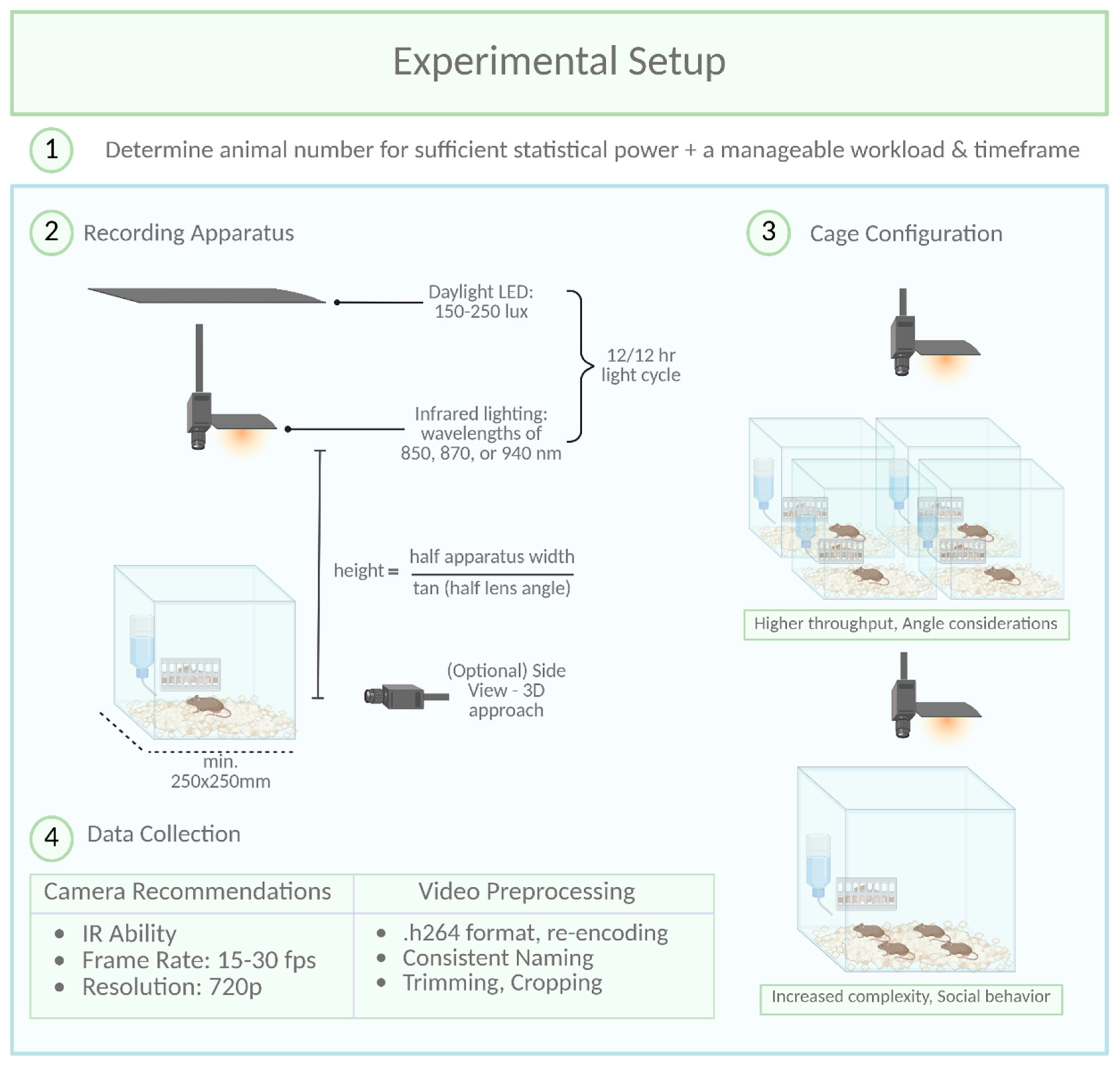
Table 1.
Non-exhaustive list of available commercial and open-source software packages, references and key features. Extended and updated from Isik & Unal 2023.
Table 1.
Non-exhaustive list of available commercial and open-source software packages, references and key features. Extended and updated from Isik & Unal 2023.
| Software Name | Reference | Tracking | Behavior | Key Features | License/Price | Platform |
|---|---|---|---|---|---|---|
| ANY-maze (Stoelting) | - | yes | yes | Video tracking, contrast-based, customizable zones and parameters | Commercial | Windows, MacOS, Linux |
| EthoVision (Noldus) | Noldus, Spink, Tegelenbosch 2001 | yes | yes | Video tracking, contrast-based, customizable zones and parameters, multi-subject tracking | Commercial | Windows, MacOS, Linux |
| VideoTrack (ViewPoint) | - | yes | yes | High-precision tracking, zone tracking, activity measurements, behavioral event detection, social interaction add-on | Commercial | Windows, MacOS, Linux |
| Smart (Panlab) | - | yes | yes | phenotype characterization and behavioral analyses (locomotor activity, anxiety models, learning paradigms) | Commercial | Windows, MacOS, Linux |
| HomeCageScan (CleverSys) | - | yes | yes | Home-cage tracking, locomotion, exploration, social interactions | Commercial | Windows, MacOS, Linux |
| CinePlex (Plexon) | - | yes | yes | Behavioral tracking integrates with neural recordings, 2 and 3D tracking, Y- T- Water-, and Plusmaze tracking | Commercial | Windows, MacOS, Linux |
| DeepLabCut | (Mathis et al., 2018) | yes | no | 2D/3D pose estimation, high-precision tracking of body parts, deep learning | Open-Source (Free) | Python Package |
| DeepOF | (Bordes et al., 2023) | no | yes | supervised and unsupervised analysis pipeline, single or multi-animal, any shape of arena, uses SHAP scores | Open-Source (Free) | Python Package |
| SLEAP (Social LEAP Estimates Animal Poses) | (Pereira et al., 2022) | yes | no | Multi-animal tracking, pose estimation, behavioral analysis using deep learning | Open-Source (Free) | Python Package |
| SimBA | (Goodwin et al., 2024) | no | yes | intuitive GUI, user can generate classifiers for behaviors and arenas, uses SHAP scores | Open-Source (Free) | Python Package |
| DeepPoseKit | (Graving et al., 2019) | yes | no | single animal tracking, fast and easy-to-use, possible to load data from DLC | Open-Source (Free) | Python Package |
| DANNCE (3-Dimensional Aligned Neural Network for Computational Ethology) | (Dunn et al., 2021) | yes | no | tracks well in 3D environments where animals can be occluded, works with multiple species | Open-Source (Free) | Python Package |
| MARS | (Segalin et al., n.d.) | yes | yes | Social interaction | Open-Source (Free) | Python Package |
| JARVIS (Markerless 3D Motion Capture Toolbox) | - | yes | no | 3D pose estimation | Open-Source (Free) | Python Package |
| AlphaTracker (multi-animal tracking and behavioral analysis tool) | (Chen et al., 2023) | yes | yes | unsupervised analysis, webcam-based video sources, tracks multiple animals | Open-Source (Free) | Python Package |
| TRex | (Walter & Couzin, 2021) | yes | no | multiple animals (~256 individuals), fast tracking for long videos | Open-Source (Free) | written in C++, but Python interface |
| OptiFlex | (Liu et al., 2021) | yes | no | Multi-Frame Animal Pose Estimation Combining Deep Learning With Optical Flow | Open-Source (Free) | Python Package |
| B-SOID | (Hsu & Yttri, 2021) | no | yes | unsupervised analysis, millisecond resolution of behavior | Open-Source (Free) | Python Package |
| Mo-Seq | (Wiltschko et al., 2020) | no | yes | unsupervised analysis, behavioral syllables | Open-Source (Free) | Python Package |
| LightningPose | (Biderman et al., 2024) | yes | no | semi-supervised learning with Bayesian tools | Open-Source (Free) | Python Package |
| SuperAnimal | (Ye et al., 2024) | yes | no | builds unifying models across differently labeled datasets | Open-Source (Free) | Python Package |
| BehaviorDEPOT | (Gabriel et al., 2022) | no | yes | freezing detection, multiple test arenas | Open-Source (Free) | MATLAB |
| Behavior Atlas | (Huang et al., 2021) | no | yes | unsupervised analysis | Open-Source (Free) | MATLAB |
| DeepAction | (Harris et al., 2023) | no | yes | Homecage monitoring | Open-Source (Free) | MATLAB |
| DeepEthogram | (Bohnslav et al., 2021) | no | yes | OFT, EPM, FST, social interaction | Open-Source (Free) | Python Package |
| MiceProfiler | (de Chaumont et al., 2012) | yes | yes | Social interaction, sniffing, chase, escape | Open-Source (Free) | Icy |
| 3DTracker | (Matsumoto et al., 2013) | yes | yes | Social interaction with manual correction, developed for rats | Open-Source (Free) | MATLAB |
| Boris (Behavioral Observation Research Interactive Software) | (Friard & Gamba, 2016) | yes | yes | possibility to include audio spectrograms | Open-Source (Free) | Python Package |
Table 2.
Parameters setup for training and inference pipeline within multi-animal top-down model type in SLEAP.ai. The set is prepared with relation to a square box setup of 50cm x 50cm dim., grayscale 648x600px recordings with very little noise introduced and mice as tracking subjects.
Table 2.
Parameters setup for training and inference pipeline within multi-animal top-down model type in SLEAP.ai. The set is prepared with relation to a square box setup of 50cm x 50cm dim., grayscale 648x600px recordings with very little noise introduced and mice as tracking subjects.
| Centroid Model Configuration | Centered Instance Model Configuration | ||
|---|---|---|---|
| Data | Validation fraction | 0.1 | 0.1 |
| Input Scaling | 0.75 | 1 | |
| Crop Size | Auto | 144 (Auto) | |
| Optimization | Batch Size | 4 | 4 |
| Epochs | 100 | 200 | |
| Initial Learning Rate | 0.0001 | 0.0001 | |
| Stop Training on Plateau | disabled | disabled | |
| Plateau Min. Delta | 1.00E-08 | 1.00E-08 | |
| Plateau Patience | 20 | 10 | |
| Online Mining | disabled | enabled | |
| Min Hard Keypoints | - | 1 | |
| Max Hard Keypoints | - | none | |
| Augmentation | Rotate | enabled | enabled |
| Rotation Min Angle | -180 | -180 | |
| Rotation Max Angle | 180 | 180 | |
| Scale | disabled | disabled | |
| Scale Min | - | - | |
| Scale Max | - | - | |
| Random flip | none | none | |
| Uniform Noise | disabled | disabled | |
| Uniform Noise Min Val | - | - | |
| Uniform Noise Max Val | - | - | |
| Gaussian Noise | disabled | disabled | |
| Gaussian Noise Mean | - | - | |
| Gaussian Nose Stddev | - | - | |
| Contrast | enabled | enabled | |
| Contrast Min Gamma | 0.5 | 0.5 | |
| Contrast Max Gamma | 2 | 2 | |
| Brightness | enabled | enabled | |
| Brightness Min Val | 0 | 0 | |
| Brightness Max Val | 10 | 10 | |
| Model | Backbone | unet | unet |
| Stem Stride | none | none | |
| Max Stride | 16 | 16 | |
| Filters | 16 | 24 | |
| Filters Rate | 2 | 2 | |
| Middle Block | enabled | enabled | |
| Up Interpolate | enabled | enabled | |
| Heads | centroid | centered_instance | |
| Anchor Part | (animal center point) | (animal center point) | |
| Sigma | 2.5 | 2.5 | |
| Output Stride | 2 | 4 |
Table 3.
General parameters setup for model training within multi-animal top-down model type in SLEAP.ai.
Table 3.
General parameters setup for model training within multi-animal top-down model type in SLEAP.ai.
| Training Pipeline | |
|---|---|
| Training/Inference Pipeline Type | multi-animal top-down |
| Max Instances | (number of animals in a box) |
| Sigma for Centroids | 2.5 |
| Anchor Part | (animal center point) |
| Sigma for Nodes | 2.5 |
| Best Model | selected |
| Latest Model | deselected |
| Final Model | deselected |
Table 4.
General parameters setup for inference within multi-animal top-down model type in SLEAP.ai.
Table 4.
General parameters setup for inference within multi-animal top-down model type in SLEAP.ai.
| Inference Pipeline | |
|---|---|
| Training/Inference Pipeline Type | multi-animal top-down |
| Max Instances | (number of animals in a box) |
| Tracker (cross-frame identity) Method | simple |
| Max numer of tracks | (number of animals in a box) |
| Similarity Method | iou |
| Matching Method | hungarian |
| Elapsed Frame Window | 5 |
| Robust quantile of similarity scope | Use max |
| Enable Filters after Initial Frames | Don’t use filters |
| Nodes to use for Tracking | (all animal keypoints) |
| Connect Single Track Breaks | enabled |
| Predict On | (entire video of choice) |
Disclaimer/Publisher’s Note: The statements, opinions and data contained in all publications are solely those of the individual author(s) and contributor(s) and not of MDPI and/or the editor(s). MDPI and/or the editor(s) disclaim responsibility for any injury to people or property resulting from any ideas, methods, instructions or products referred to in the content. |
© 2025 by the authors. Licensee MDPI, Basel, Switzerland. This article is an open access article distributed under the terms and conditions of the Creative Commons Attribution (CC BY) license (http://creativecommons.org/licenses/by/4.0/).
Copyright: This open access article is published under a Creative Commons CC BY 4.0 license, which permit the free download, distribution, and reuse, provided that the author and preprint are cited in any reuse.


