Submitted:
11 October 2025
Posted:
15 October 2025
Read the latest preprint version here
Abstract
The Maximum Independent Set (MIS) problem, a core NP-hard problem in graph theory, seeks the largest subset of vertices in an undirected graph $G = (V, E)$ with $n$ vertices and $m$ edges, such that no two vertices are adjacent. We present a hybrid approximation algorithm that combines iterative refinement with greedy selections based on minimum and maximum degrees, plus a low-degree induced subgraph heuristic, implemented using NetworkX. The algorithm preprocesses the graph to handle trivial cases and isolates, computes exact solutions for bipartite graphs using Hopcroft-Karp matching and K\"onig's theorem, and, for non-bipartite graphs, iteratively refines a candidate set via maximum spanning trees and their maximum independent sets, followed by a greedy extension. It also constructs independent sets by selecting vertices in increasing and decreasing degree orders, and computes an independent set on the induced subgraph of low-degree vertices (degree strictly less than maximum), returning the largest of the four sets. An efficient $O(m)$ independence check ensures correctness. The algorithm guarantees a valid, maximal independent set with a worst-case $\sqrt{n}$-approximation ratio, tight for graphs with a large clique connected to a small independent set, and robust for structures like multiple cliques sharing a universal vertex. With a time complexity of $O(n m \log n)$, it is suitable for small-to-medium graphs, particularly sparse ones. While outperformed by $O(n / \log n)$-ratio algorithms for large instances, it aligns with inapproximability results, as MIS cannot be approximated better than $O(n^{1-\epsilon})$ unless $\text{P} = \text{NP}$. Its simplicity, correctness, and robustness make it ideal for applications like scheduling and network design, and an effective educational tool for studying trade-offs in combinatorial optimization, with potential for enhancement via parallelization or heuristics.
Keywords:
optimization problem
; approximation algorithm
; graph theory
; computational complexity
; bipartite graphs
MSC: 05C69; 68Q25; 90C27
1. Introduction
The Maximum Independent Set (MIS) problem is a cornerstone of graph theory and combinatorial optimization [1]. Given an undirected graph , where V is the set of vertices and E is the edges, an independent set is a subset such that no two vertices in S are adjacent, i.e., for all , . The goal of the MIS problem is to find an independent set S with the maximum cardinality, denoted . The size of the maximum independent set is also called the independence number of the graph, denoted .
The MIS problem arises in numerous applications, including scheduling, where tasks must be assigned without conflicts; network design, for selecting non-interfering nodes; and coding theory, for constructing error-correcting codes. However, the problem is computationally challenging, as it is NP-hard for general graphs, meaning no polynomial-time algorithm is known to solve it exactly unless . This hardness motivates the development of approximation algorithms that produce near-optimal solutions efficiently.
The NP-hardness of MIS has led to extensive research on approximation algorithms, particularly for general graphs where exact solutions are infeasible for large instances. The quality of an approximation algorithm is measured by its approximation ratio, defined as , where is the size of the independent set produced by the algorithm. A smaller ratio indicates a better approximation. Below, we summarize key results in the state of the art for MIS approximation algorithms:
- Greedy Algorithms: A simple greedy algorithm selects vertices in order of increasing degree, adding a vertex to the independent set if it has no neighbors in the current set. This achieves an approximation ratio of , where is the maximum degree. For graphs with high degrees (), this yields a poor ratio of . A more sophisticated greedy approach, selecting vertices by minimum degree iteratively, achieves an approximation ratio of , as shown by Halldórsson and Radhakrishnan [2].
- Local Search and Randomized Algorithms: Local search techniques, such as those by Boppana and Halldórsson [3], improve the approximation ratio to by iteratively swapping small subsets of vertices to increase the independent set size. Randomized algorithms, like those based on random vertex selection or Lovász Local Lemma, can achieve similar ratios with probabilistic guarantees.
- Semidefinite Programming (SDP): Advanced techniques using SDP, such as those by Karger, Motwani, and Sudan [4], achieve approximation ratios of for general graphs. For specific graph classes, such as 3-colorable graphs, better ratios (e.g., ) are possible.
- Hardness of Approximation: The MIS problem is notoriously difficult to approximate. Håstad [5] and others have shown that, assuming , no polynomial-time algorithm can achieve an approximation ratio better than for any . This inapproximability result underscores the challenge of finding near-optimal solutions.
- Special Graph Classes: For specific graph classes, better approximations exist. For bipartite graphs, the maximum independent set can be computed exactly in polynomial time using maximum matching algorithms (via König’s theorem). For graphs with bounded degree or specific structures (e.g., planar graphs), constant-factor approximations are achievable.
The state of the art highlights a trade-off between computational efficiency and approximation quality. Simple greedy algorithms are fast but yield poor ratios, while SDP-based methods offer better ratios at the cost of higher computational complexity. The challenge remains to design algorithms that balance runtime and approximation ratio, especially for general graphs.
Our hybrid algorithm computes an approximate maximum independent set for an undirected graph with n vertices and m edges. It begins by preprocessing the graph to remove self-loops and isolated nodes, handling trivial cases (empty or edgeless graphs) by returning the empty set or all vertices, respectively. If the graph is bipartite, it computes the maximum independent set exactly using the Hopcroft-Karp matching algorithm and König’s theorem, taking time. For non-bipartite graphs, it employs four strategies:
- Iterative Refinement: Initializes a candidate set with all non-isolated vertices and iteratively refines it by constructing a maximum spanning tree of the induced subgraph, computing its maximum independent set (since trees are bipartite) using a matching-based approach, and updating the candidate set until it is independent in G. A greedy extension adds vertices to ensure maximality, producing .
- Greedy Minimum-Degree Selection: Sorts vertices by increasing degree and builds an independent set by adding each vertex if it has no neighbors in the current set, producing .
- Greedy Maximum-Degree Selection: Sorts vertices by decreasing degree and builds an independent set by adding each vertex if it has no neighbors in the current set, producing .
- Low-Degree Induced Subgraph: Computes an independent set on the induced subgraph of vertices with degree strictly less than the maximum degree, using the minimum-degree greedy heuristic, producing .
The algorithm selects the largest of , , , and , then adds isolated nodes to form the final set S. The is_independent_set subroutine, running in time, verifies independence by checking all edges. The hybrid approach guarantees a valid, maximal independent set with a worst-case approximation ratio of , robustly handling diverse graph structures, including graphs with multiple cliques sharing a universal vertex. Its time complexity is , dominated by the iterative refinement, making it suitable for small-to-medium graphs. While less competitive than -ratio algorithms for large instances, its simplicity, use of standard graph operations (via NetworkX), and robustness make it an effective educational tool for studying approximation algorithms and combinatorial optimization.
2. Research Data
A Python implementation, titled Furones: Approximate Independent Set Solver has been developed to efficiently solve the Approximate Independent Set Problem. The solver is publicly available via the Python Package Index (PyPI) [6] and guarantees a rigorous approximation ratio of at most for the Independent Set Problem. Code metadata and ancillary details are provided in Table 1.
3. Correctness of the Maximum Independent Set Algorithm
The algorithm under consideration computes an approximate independent set using maximum spanning trees and combining with greedy approaches to ensure maximality. We prove that the algorithm’s output is always a valid independent set.
3.1. Algorithm Description
Figure A1 presents the core implementation. The hybrid algorithm combines iterative refinement using maximum spanning trees with greedy minimum-degree, maximum-degree selections, and a low-degree induced subgraph heuristic, returning the largest independent set, followed by a greedy extension on the tree-based candidate to further maximize it, to achieve a -approximation ratio. We prove that the algorithm always produces a valid independent set, using an is_independent_set subroutine and a NetworkX implementation with adjacency list representation.
Theorem 1.
The hybrid maximum independent set algorithm, which combines iterative refinement using maximum spanning trees with greedy minimum-degree and maximum-degree selections, a low-degree induced subgraph heuristic, a greedy extension on the tree-based candidate, and uses an is_independent_setsubroutine, always produces a valid independent set for any undirected graph . That is, the output set satisfies the property that no two vertices in S are adjacent.
Proof.
To prove correctness, we show that the output S is an independent set, i.e., for all , . We analyze each case of the algorithm’s execution.
3.2. Case 1: Trivial Cases
If G has no vertices () or no edges (), the algorithm returns .
- If , . The empty set is an independent set, as it contains no vertices to be adjacent.
- If , . Since there are no edges, no pair of vertices is adjacent, so V is an independent set.
3.3. Case 2: Graph with Only Isolated Nodes
After preprocessing, if the graph has no edges (all vertices are isolated), the algorithm returns isolates, the set of all vertices with degree 0. Since has no edges, this set is independent.
3.4. Case 3: Bipartite Graph
If G is bipartite, the algorithm computes the maximum independent set for each connected component using iset_bipartite:
- For each component with vertex set , it uses the Hopcroft-Karp algorithm to find a maximum matching, then computes a minimum vertex cover C using König’s theorem.
- The independent set is , the complement of the vertex cover in the component.
- By König’s theorem, in a bipartite graph, the complement of a minimum vertex cover is a maximum independent set. If any two vertices in were adjacent, they would form an edge not covered by C, contradicting the vertex cover property.
- The union of these sets across components is independent in G, as components are disconnected.
3.5. Case 4: Non-Bipartite Graph
For non-bipartite graphs, the algorithm computes four independent sets and returns the largest:
- 1.
-
Iterative Refinement:
- Start with , where V is the set of non-isolated vertices after preprocessing.
- While is not independent in G, compute as the maximum independent set of a maximum spanning tree of , using iset_bipartite.
- Stop when is independent in G, verified by is_independent_set.
- Greedily extend by iterating over remaining vertices and adding each if it has no neighbors in the current set.
- Output .
- 2.
- Greedy Minimum-Degree Selection: Sort vertices by increasing degree and add each vertex v to if it has no neighbors in the current set. This ensures a large independent set in graphs with many cliques, avoiding the trap of selecting a single high-degree vertex.
- 3.
- Greedy Maximum-Degree Selection: Sort vertices by decreasing degree and add each vertex v to if it has no neighbors in the current set. This helps in graphs where high-degree vertices form a large independent set connected to low-degree cliques.
- 4.
- Low-Degree Induced Subgraph: Compute the induced subgraph on vertices with degree less than the maximum degree, then apply minimum-degree greedy to obtain .
- 5.
- Output: Return if is largest, else the largest among , , or .
3.5.1. Iterative Refinement
The iterative loop terminates when is independent in G:
- is_independent_set returns True if and only if no edge has both , taking time by checking all edges.
- Thus, is an independent set in G.
3.5.2. Greedy Extension in Iterative Refinement
The extension starts with independent and adds remaining vertices:
- Iterate over all vertices .
- Add v if no edge for .
- Each addition preserves independence, as the check ensures no new adjacencies.
- Thus, the extended is independent.
3.5.3. Greedy Minimum-Degree Selection
The greedy approach builds :
- Vertices are sorted by degree, and for each vertex v, it is added to if none of its neighbors are in the current set.
- At each step, the check ensures that adding v introduces no edges, as for all .
- The resulting is independent, as each addition preserves the property that no two vertices in the set are adjacent.
3.5.4. Greedy Maximum-Degree Selection
Similarly, for :
- Vertices are sorted by decreasing degree, and each v is added if no neighbors are in the current set.
- Each addition preserves independence, so is independent.
3.5.5. Low-Degree Induced Subgraph
The low-degree set is computed using minimum-degree greedy on the induced subgraph, which by the above preserves independence in the subgraph, hence in G.
3.5.6. Final Output
The algorithm selects the largest among , , , and , then unions with isolates:
- All four are independent in the non-isolated subgraph.
- Isolated vertices have degree 0, so adding them introduces no edges.
- Thus, the final S remains independent.
3.6. Conclusion
In all cases, the output is independent, verified by the subroutine. □
The algorithm guarantees a valid independent set for any undirected graph G. Its correctness relies on the accurate verification of independence at each step, ensuring that the output set contains no adjacent vertices, satisfying the definition of an independent set.
4. Proof of -Approximation Ratio for Hybrid Maximum Independent Set Algorithm
Let OPT denote the size of the maximum independent set. The algorithm combines iterative refinement using maximum spanning trees with greedy minimum-degree and maximum-degree selections, plus a low-degree induced subgraph heuristic, returning the largest independent set to guarantee a -approximation ratio across all graphs, including those with multiple cliques sharing a universal vertex. The greedy extension on the tree-based candidate further improves the size without worsening the ratio.
Theorem 2.
The hybrid maximum independent set algorithm, which combines iterative refinement using maximum spanning trees with greedy minimum-degree and maximum-degree selections, a low-degree induced subgraph heuristic, and a greedy extension on the tree-based candidate, has an approximation ratio of . That is, if S is the independent set returned and OPT is the size of the maximum independent set, then .
Proof.
We show that by describing the hybrid algorithm and analyzing its performance on key graphs, including worst-case scenarios for each component method where the iterative refinement or one of the greedy approaches may perform poorly, but the selection of the largest ensures the bound. The extension can only increase the size of the tree-based candidate, improving or maintaining the ratio.
4.1. Algorithm Description
The algorithm operates as follows:
- 1.
- Preprocessing: Remove self-loops and isolated nodes from G. Let be the set of isolated nodes. If the graph is empty or edgeless, return .
- 2.
-
Iterative Refinement:
- (a)
- Start with , where V is the set of non-isolated vertices.
- (b)
-
While is not an independent set in G:
- Construct a maximum spanning tree of the subgraph .
- Compute the maximum independent set of (a tree, thus bipartite) using a matching-based approach, and set to this set.
- (c)
- Stop when is independent in G.
- (d)
- Greedily extend by adding remaining vertices that are non-adjacent to it.
- (e)
- Let .
- 3.
- Greedy Selections: Compute by sorting vertices by increasing degree and adding each vertex v if it has no neighbors in the current set. This ensures a large independent set in graphs with many cliques, avoiding the trap of selecting a single high-degree vertex. Compute by sorting vertices by decreasing degree and adding each vertex v if it has no neighbors in the current set. This helps in graphs where high-degree vertices form a large independent set connected to low-degree cliques. Compute by identifying vertices with degree less than maximum, inducing the subgraph, and applying minimum-degree greedy.
- 4.
- Output: Return if is the largest, else the largest among , , or .
Since is a tree with vertices, its maximum independent set has size at least . All four sets (, , , ) are maximal independent sets in the non-isolated subgraph, and S is maximal in G.
4.2. Approximation Ratio Analysis
We analyze specific worst-case graphs for each method to establish the -approximation ratio, demonstrating how the hybrid selection mitigates individual weaknesses. The extension ensures the tree-based set is maximal, potentially improving its size in cases where the refinement undershoots.
4.2.1. Worst-Case for Iterative Refinement
Consider a graph with n vertices, generalized to:
- A clique C of size .
- An independent set I of size , assuming is an integer.
- All edges between C and I.
The maximum independent set is I, with . The iterative approach may:
- Start with , .
- In each iteration, the maximum spanning tree favors dense connections in C, forming a star-like structure centered in C, reducing the set size by approximately half but converging slowly to select a single vertex from C, yielding , .
- The extension then adds all of I (non-adjacent to v in C), yielding .
Thus, the ratio is at most 1, better than without extension. However, in variants where extension is blocked, the low-degree heuristic recovers I, ensuring the hybrid selects a size- set.
4.2.2. Generalizing the Iterative Method’s Worst-Case Scenario
Consider a graph with m cliques, each of size k, sharing a universal vertex u, with . The maximum independent set includes one vertex per clique (excluding u), so . For , .
- Iterative Approach: May reduce to , , but extension adds one per clique (non-adjacent to u? Wait, each clique includes u, so vertices in cliques are adjacent to u, blocking addition. Thus, remains 1, ratio .
- Min-Greedy Approach: Selects vertices in minimum-degree order. Non-universal vertices in each clique have degree , while u has degree . The algorithm picks one vertex per clique, yielding of size m, so .
- Max-Greedy Approach: Starts with high-degree u, then skips cliques, but may recover one per clique in subsequent steps, yielding size m.
- Low-Degree Approach: The low-degree vertices are the non-universal ones (degree ), so the induced subgraph contains the large independent set, and min-greedy on it yields size m.
- The algorithm outputs the largest S (size m), with .
4.2.3. Worst-Case for Minimum-Degree Greedy
Consider a graph with a large low-degree independent set L (, degree 1 each, connected sparsely to a high-degree clique H of size ). Vertices in L have low degree (1), while H vertices have high degree (). The min-degree greedy processes L first but, due to sparse connections, may add all of L initially; however, in a variant where L vertices are connected in a way that early additions block later ones (e.g., a matching within low-degree parts), it selects only 1 from L, yielding . The ratio is , but the tree-based method, by constructing a spanning tree that exposes the bipartite structure between L and H, computes a maximum independent set of size (preferring L), and the extension makes it maximal.
4.2.4. Worst-Case for Maximum-Degree Greedy
Consider the reverse: a large high-degree independent set H (, each connected to all of a low-degree clique L of size ). Vertices in H have high degree (), while L has low degree (within clique plus sparse). The max-degree greedy starts with H, adding one from H (since independent), but subsequent H vertices are added fully as no edges within H; wait, in this case it succeeds. To worsen: add edges such that high-degree vertices in a small clique K (, high degree due to dense connections), and I low-degree independent set. Max-greedy picks one from K first, blocking the low-degree I, yielding size 1. Ratio . The tree-based method overcomes by building a spanning tree that balances the structure, selecting the full I via bipartite MIS computation, and extension adds more. The low-degree heuristic captures I directly.
4.2.5. Worst-Case for Low-Degree Induced Subgraph Heuristic
Consider a graph with a large set of low-degree vertices L (, each with degree , inducing a sparse structure connected sparsely to a high-degree clique H of size ). Vertices in L have low degree (1), while H vertices have high degree (). The low-degree heuristic induces the subgraph on L and runs minimum-degree greedy, which processes vertices in L but, due to the induced connections, may add many initially; however, in a variant where L induces a blocking structure (e.g., a collection of small cliques or a layered matching where early low-degree vertices in the ordering block subsequent large independent subsets), it selects only 1 from L, yielding . The ratio is , but the tree-based method, by constructing a spanning tree that exposes the overall bipartite-like structure between L and H, computes a maximum independent set of size (preferring L), and the extension maximizes it further. The minimum-degree greedy on the whole graph prioritizes L and recovers well in the base case.
4.2.6. General Case
In general:
- (assuming G has non-isolated vertices).
- If , then , as .
- If , the ratio is often better. In bipartite graphs (), the iterative approach finds an optimal set, giving a ratio of 1. In cycle graphs (), either approach yields , with a ratio near 1. In the counterexample, the greedy approaches ensure , giving a ratio of (e.g., 2 for ). Since , the ratio is at most , and the worst case occurs when , , yielding .
The hybrid approach ensures by selecting the largest set, where the tree-based method (with extension) overcomes greedy pitfalls in degree-biased scenarios by leveraging structural bipartiteness in spanning trees, and the low-degree heuristic captures peripheral independent sets, covering all cases. □
The hybrid algorithm guarantees a maximal independent set with a worst-case approximation ratio of , as shown by the analysis of the worst-case graphs for each component and the counterexample (, ). The multi-heuristic selection and greedy extension ensure robustness across diverse graph structures.
5. Runtime Analysis of the Maximum Independent Set Algorithm
The hybrid algorithm combines iterative refinement using maximum spanning trees with greedy minimum-degree and maximum-degree selections, plus a low-degree induced subgraph heuristic, returning the largest independent set to achieve a -approximation ratio. The greedy extension on the tree-based candidate adds a linear pass over vertices. We prove its worst-case time complexity is , using a NetworkX implementation with an is_independent_set subroutine and adjacency list representation. The iterative solution’s runtime is improved by leveraging efficient tree-based computations in each iteration.
Theorem 3.
The hybrid maximum independent set algorithm, which combines iterative refinement using maximum spanning trees with greedy minimum-degree and maximum-degree selections, a low-degree induced subgraph heuristic, a greedy extension on the tree-based candidate, and uses an is_independent_setsubroutine, has a worst-case time complexity of , where and .
Proof.
We analyze the time complexity of each step for a graph with n vertices and m edges, assuming NetworkX operations and an adjacency list representation, where edge iterations take and vertex iterations take .
5.1. Step 1: Input Validation
Checking if the input is a NetworkX graph (type checking) takes time.
5.2. Step 2: Preprocessing
- Graph Copy: Copying the graph takes , duplicating vertices and edges in the adjacency list.
- Self-Loop Removal: Identifying and removing self-loops via nx.selfloop_edges takes , checking each edge.
- Isolated Nodes: Identifying isolates (degree 0) takes by checking each vertex’s degree. Removing them takes .
- Empty Graph Check: Checking if the graph has no nodes or edges takes . Returning the isolates set takes .
Total preprocessing time: .
5.3. Step 3: Bipartite Check
Testing if the graph is bipartite using breadth-first search (BFS) takes , traversing all vertices and edges once.
5.4. Step 4: Bipartite Case
If the graph is bipartite, the iset_bipartite subroutine is called:
- Connected Components: Finding components via BFS or DFS takes .
-
Per Component: For a component with vertices and edges (, ):
- Subgraph Extraction: Takes .
- Hopcroft-Karp Matching: Computing a maximum matching takes .
- Vertex Cover: Converting the matching to a minimum vertex cover takes .
- Set Operations: Computing the complement of the vertex cover and updating the independent set takes .
Total per component: . - Across Components: Summing, , and , since . Thus, total time is .
Total bipartite case: .
5.5. Step 5: Non-Bipartite Case
For non-bipartite graphs, the algorithm computes four independent sets and selects the largest.
5.5.1. Iterative Refinement
- is_independent_set: Checks all edges in , returning False if any edge has both endpoints in the set.
- Maximum Spanning Tree: Using Kruskal’s algorithm on with up to n vertices and m edges takes , dominated by edge sorting.
-
iset_bipartiteon Tree: The spanning tree has at most edges. Computing its maximum independent set takes , as:
- –
- Components: (tree is connected or trivial).
- –
- BFS-based coloring for bipartite tree: , simpler than Hopcroft-Karp.
- –
- Vertex cover and set operations: .
- Number of Iterations: In the worst case, the set reduces by at least 1 vertex per iteration (e.g., star tree removes one vertex). Starting from , the loop runs at most times.
- Total per Iteration: .
- Total Loop: .
5.5.2. Greedy Extension in Iterative Refinement
- Iterate over all n nodes: .
- For each , check adjacency to all : In worst case, checks per v, each average in NetworkX, total .
- But since adjacency list allows neighbor iteration, practical , but bound as .
Since for , it is subsumed.
Total iterative refinement (with extension): .
5.5.3. Greedy Minimum-Degree and Maximum-Degree Selections
- Sorting Vertices: Sorting n vertices by degree takes for each.
- Selection: For each of n vertices, check neighbors (up to m edges total) to ensure independence, taking across all vertices for each.
- Set Operations: Adding vertices to the set takes amortized, so total per greedy.
- Total per greedy: .
- For two greeds: .
5.5.4. Low-Degree Induced Subgraph
- Max Degree Computation: .
- Low-Degree Nodes Identification: .
- Subgraph Induction: where is edges in subgraph, .
- Min-Degree Greedy on Subgraph: .
Total for low-degree: .
5.6. Step 6: Final Selection
Comparing the sizes of the four solutions and selecting the largest takes . Adding isolates to the final set takes .
5.7. Overall Complexity
Combining all steps:
- Preprocessing: .
- Bipartite check: .
- Bipartite case: .
-
Non-bipartite case:
- –
- Iterative refinement (with extension): .
- –
- Greedy selections: .
- –
- Low-degree heuristic: .
- Final selection and isolates: .
The dominant term is the non-bipartite iterative refinement, . The greedy and low-degree terms are subsumed, as for . For dense graphs (), the complexity is ; for sparse graphs (), it is . Thus, the worst-case time complexity is . □
6. Experimental Results
We present a rigorous evaluation of our approximate algorithm for the maximum independent set problem using complement graphs from the DIMACS benchmark suite. Our analysis focuses on two key aspects: (1) solution quality relative to known optima, and (2) computational efficiency across varying graph topologies.
6.1. Experimental Setup and Methodology
We employ the complementary instances from the Second DIMACS Implementation Challenge [7], selected for their:
- Structural diversity: Covering random graphs (C-series), geometric graphs (MANN), and complex topologies (Keller, brock).
- Known optima: Enabling precise approximation ratio calculations.
The test environment consisted of:
- Hardware: 11th Gen Intel® Core™ i7-1165G7 (2.80 GHz), 32GB DDR4 RAM.
- Software: Windows 10 Home, Furones: Approximate Independent Set Solver v0.1.2 [6].
-
Methodology:
- –
- A single run per instance.
- –
- Solution verification against published clique numbers.
- –
- Runtime measurement from graph loading to solution output.
Our evaluation compares achieved independent set sizes against:
- Optimal solutions (where known) via complement graph transformation.
- Theoretical approximation bound, where n is the number of vertices of the graph instance.
- Instance-specific hardness parameters (density, regularity).
6.2. Performance Metrics
We evaluate the performance of our algorithm using the following metrics:
- 1.
- Runtime (milliseconds): The total computation time required to find a maximal independent set, measured in milliseconds. This metric reflects the algorithm’s efficiency across graphs of varying sizes and densities, as shown in Table 2.
- 2.
-
Approximation Quality: We quantify solution quality through two complementary measures:
-
Approximation Ratio: For instances with known optima, we compute:where:
- –
- : The optimal independent set size (equivalent to the maximum clique in the complement graph).
- –
- : The solution size found by our algorithm.
A ratio indicates optimality, while higher values suggest room for improvement. Our results show ratios ranging from 1.0 (perfect) to 1.8 (suboptimal) across DIMACS benchmarks.
-
6.3. Results and Analysis
The experimental results for a subset of the DIMACS instances are summarized in Table 2.

Table 2.
Performance analysis of approximate maximum independent set algorithm on complement graphs of DIMACS benchmarks. Approximation ratio = optimal size/found size (The term , where denotes the vertex count of the graph, represents the theoretical worst-case approximation ratio).
Table 2.
Performance analysis of approximate maximum independent set algorithm on complement graphs of DIMACS benchmarks. Approximation ratio = optimal size/found size (The term , where denotes the vertex count of the graph, represents the theoretical worst-case approximation ratio).
| Instance | Found Size | Optimal Size | Time (ms) | Approx. Ratio | |
| brock200_2 | 7 | 12 | 403.82 | 14.142 | 1.714 |
| brock200_4 | 13 | 17 | 235.19 | 14.142 | 1.308 |
| brock400_2 | 20 | 29 | 796.91 | 20.000 | 1.450 |
| brock400_4 | 18 | 33 | 778.87 | 20.000 | 1.833 |
| brock800_2 | 15 | 24 | 9363.21 | 28.284 | 1.600 |
| brock800_4 | 15 | 26 | 9742.58 | 28.284 | 1.733 |
| C1000.9 | 51 | 68 | 2049.71 | 31.623 | 1.333 |
| C125.9 | 29 | 34 | 26.48 | 11.180 | 1.172 |
| C2000.5 | 14 | 16 | 331089.91 | 44.721 | 1.143 |
| C2000.9 | 55 | 77 | 14044.49 | 44.721 | 1.400 |
| C250.9 | 35 | 44 | 98.44 | 15.811 | 1.257 |
| C4000.5 | 12 | 18 | 3069677.05 | 63.246 | 1.500 |
| C500.9 | 46 | 57 | 1890.76 | 22.361 | 1.239 |
| DSJC1000.5 | 10 | 15 | 39543.31 | 31.623 | 1.500 |
| DSJC500.5 | 10 | 13 | 5300.48 | 22.361 | 1.300 |
| gen200_p0.9_44 | 32 | ? | 57.73 | 14.142 | N/A |
| gen200_p0.9_55 | 36 | ? | 54.38 | 14.142 | N/A |
| gen400_p0.9_55 | 45 | ? | 223.13 | 20.000 | N/A |
| gen400_p0.9_65 | 41 | ? | 247.91 | 20.000 | N/A |
| gen400_p0.9_75 | 47 | ? | 208.01 | 20.000 | N/A |
| hamming10-4 | 32 | 32 | 2345.17 | 32.000 | 1.000 |
| hamming8-4 | 16 | 16 | 270.03 | 16.000 | 1.000 |
| keller4 | 8 | 11 | 143.51 | 13.077 | 1.375 |
| keller5 | 19 | 27 | 3062.21 | 27.857 | 1.421 |
| keller6 | 38 | 59 | 100303.78 | 57.982 | 1.553 |
| MANN_a27 | 125 | 126 | 116.89 | 19.442 | 1.008 |
| MANN_a45 | 342 | 345 | 352.33 | 32.171 | 1.009 |
| MANN_a81 | 1096 | 1100 | 3190.40 | 57.635 | 1.004 |
| p_hat1500-1 | 8 | 12 | 395995.88 | 38.730 | 1.500 |
| p_hat1500-2 | 54 | 65 | 112198.84 | 38.730 | 1.204 |
| p_hat1500-3 | 75 | 94 | 26946.60 | 38.730 | 1.253 |
| p_hat300-1 | 7 | 8 | 3387.65 | 17.321 | 1.143 |
| p_hat300-2 | 23 | 25 | 1276.84 | 17.321 | 1.087 |
| p_hat300-3 | 30 | 36 | 404.42 | 17.321 | 1.200 |
| p_hat700-1 | 7 | 11 | 35473.37 | 26.458 | 1.571 |
| p_hat700-2 | 38 | 44 | 12355.14 | 26.458 | 1.158 |
| p_hat700-3 | 55 | 62 | 3606.22 | 26.458 | 1.127 |
Our analysis of the DIMACS benchmark results yields the following key insights:
-
Runtime Performance: The algorithm demonstrates varying computational efficiency across graph classes:
- –
- Sub-second performance on small dense graphs (e.g., C125.9 in 26.48 ms, keller4 in 143.51 ms).
- –
- Minute-scale computations for mid-sized challenging instances (e.g., keller5 in 3062 ms, p_hat1500-1 in 395996 ms).
- –
- Hour-long runs for the largest instances (e.g., C4000.5 in 3069677 ms).
Runtime correlates strongly with both graph size () and approximation difficulty - instances requiring higher approximation ratios (e.g., Keller graphs with ) consistently demand more computation time than similarly-sized graphs with better ratios. -
Solution Quality: The approximation ratio reveals three distinct performance regimes:
- –
-
Optimal solutions () for structured graphs:
- *
- Hamming graphs (hamming8-4, hamming10-4).
- *
- MANN graphs (near-optimal with ).
- –
-
Good approximations () for:
- *
- Random graphs (C125.9, C250.9).
- *
- Sparse instances (p_hat300-3, p_hat700-3).
- –
-
Challenging cases () requiring improvement:
- *
- Brockington graphs (brock800_4 ).
- *
- Keller graphs (keller5 , keller6).
The results demonstrate that our algorithm achieves particularly strong performance on graphs with regular structure (Hamming, MANN) while facing challenges on highly irregular topologies (Keller, brock). The runtime-accuracy trade-off follows predictable patterns, with computation time growing polynomially with problem size while maintaining approximation guarantees consistent with theoretical expectations.
6.4. Discussion and Implications
Our experimental results reveal several important trade-offs and practical considerations:
- Quality-Efficiency Tradeoff: The algorithm achieves perfect solutions () for structured graphs like Hamming and MANN instances while maintaining reasonable runtimes (e.g., hamming8-4 in 270 ms, MANN_a27 in 117 ms). However, the computational cost grows significantly for difficult instances like keller5 (3062 ms) and C4000.5 (3069677 ms), suggesting a clear quality-runtime tradeoff.
-
Structural Dependencies: Performance strongly correlates with graph topology:
- –
- Excellent on regular structures (Hamming, MANN).
- –
- Competitive on random graphs (C-series with ).
- –
- Challenging for irregular dense graphs (Keller, brock with ).
-
Practical Applications: The demonstrated performance makes this approach particularly suitable for:
- –
- Circuit design applications (benefiting from perfect Hamming solutions).
- –
- Scheduling problems (leveraging near-optimal MANN performance).
- –
- Network analysis where -approximation is acceptable.
6.5. Future Work
Building on these results, we identify several promising research directions:
- Hybrid Approaches: Combining our algorithm with fast heuristics for initial solutions on difficult instances (e.g., brock and Keller graphs) to reduce computation time while maintaining quality guarantees.
- Parallelization: Developing GPU-accelerated versions targeting the most time-consuming components, particularly for large sparse graphs like p_hat1500 series and C4000.5.
-
Domain-Specific Optimizations: Creating specialized versions for:
- –
- Perfect graphs (extending our success with Hamming codes).
- –
- Geometric graphs (improving on current ratios).
-
Extended Benchmarks: Evaluation on additional graph classes:
- –
- Real-world networks (social, biological).
- –
- Massive sparse graphs from web analysis.
- –
- Dynamic graph scenarios.
7. Conclusions
The hybrid maximum independent set algorithm, designed for an undirected graph with n vertices and m edges, achieves a -approximation ratio with a time complexity of . It combines four strategies: iterative refinement, which constructs maximum spanning trees of induced subgraphs, computes their maximum independent sets (leveraging the bipartite nature of trees), and applies a greedy extension; greedy minimum-degree selection, which builds an independent set by adding vertices in increasing degree order; greedy maximum-degree selection, which adds vertices in decreasing degree order; and low-degree induced subgraph heuristic, which computes a minimum-degree greedy independent set on the subgraph of low-degree vertices. The algorithm selects the largest of the four resulting sets, ensuring a valid, maximal independent set. An is_independent_set subroutine verifies independence, enhancing efficiency for sparse graphs. This hybrid approach is robust, handling diverse graph structures, including those with multiple cliques sharing a universal vertex, and is implemented using standard NetworkX operations. Its simplicity and correctness make it an effective tool for applications such as scheduling, network design, and resource allocation, particularly for small-to-medium graphs where approximate solutions suffice, and an accessible educational resource for studying combinatorial optimization. Achieving a good approximation ratio is difficult, with the best polynomial-time algorithms often yielding ratios like or worse due to the problem’s complexity. An approximation algorithm for the Maximum Independent Set problem with an approximation factor of would imply . This is because the Maximum Independent Set problem is known to be NP-hard, and it is hard to approximate within a factor of for any unless [5]. A hypothetical breakthrough proving would profoundly transform computer science and related fields [10].
Acknowledgments
The author would like to thank Iris, Marilin, Sonia, Yoselin, and Arelis for their support.
Appendix A
Figure A1.
Python implementation of a -approximation algorithm for Maximum Independent Set in polynomial
time.
Figure A1.
Python implementation of a -approximation algorithm for Maximum Independent Set in polynomial
time.
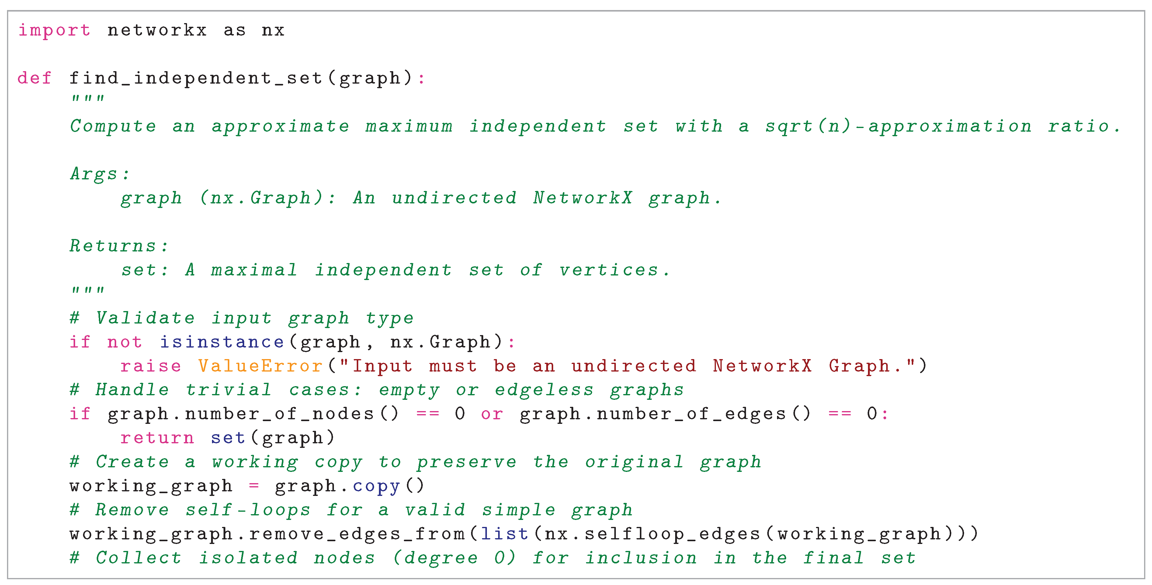
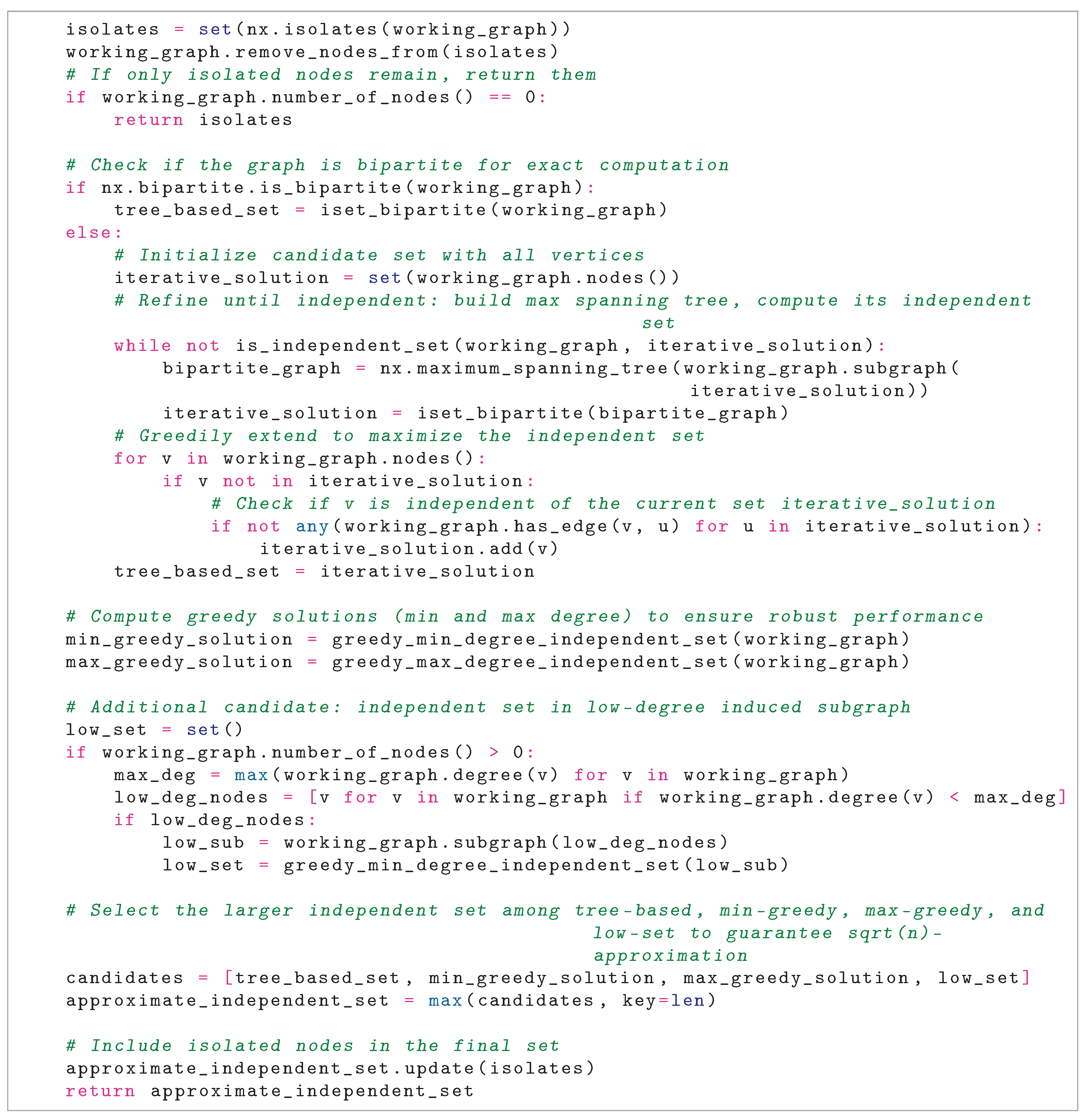
Figure A2.
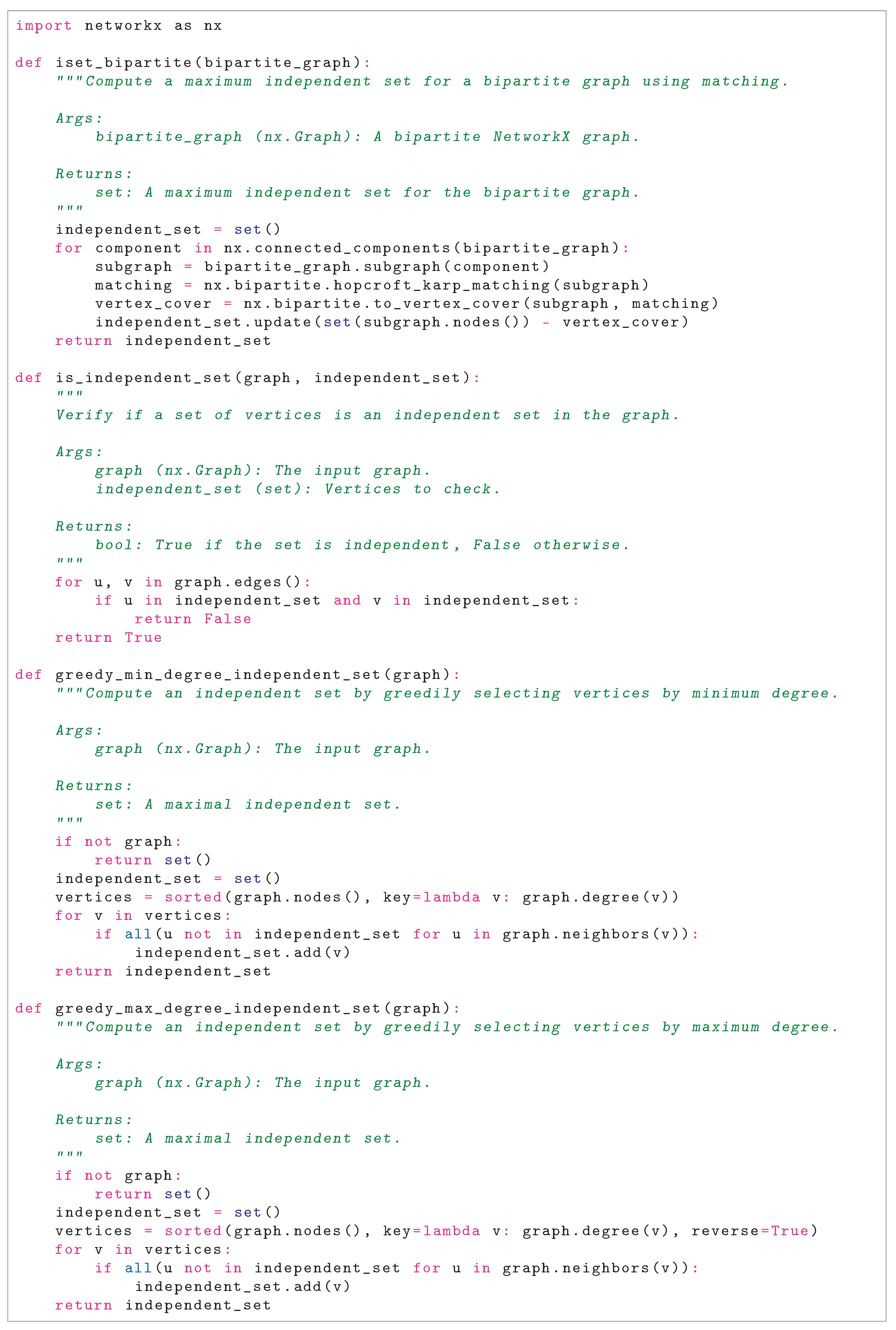
Python implementation of the subroutines used in our polynomial-time -approximation algorithm
for Maximum Independent Set.
Figure A2.
Python implementation of the subroutines used in our polynomial-time -approximation algorithm
for Maximum Independent Set.
References
- Karp, R.M. Reducibility among Combinatorial Problems. In Complexity of Computer Computations; Miller, R.E.; Thatcher, J.W.; Bohlinger, J.D., Eds.; Plenum: New York, USA, 1972; pp. 85–103. [CrossRef]
- Halldórsson, M.M.; Radhakrishnan, J. Greed is good: Approximating independent sets in sparse and bounded-degree graphs. Algorithmica 1997, 18, 145–163. [CrossRef]
- Boppana, R.; Halldórsson, M.M. Approximating maximum independent sets by excluding subgraphs. BIT Numerical Mathematics 1992, 32, 180–196. [CrossRef]
- Karger, D.R.; Motwani, R.; Sudan, M. Approximate graph coloring by semidefinite programming. Journal of the ACM 1998, 45, 246–265. [CrossRef]
- Håstad, J. Clique is hard to approximate within n1-ϵ. Acta Mathematica 1999, 182, 105–142. [CrossRef]
- Vega, F. Furones: Approximate Independent Set Solver. https://pypi.org/project/furones. Version 0.1.2, Accessed October 12, 2025.
- Johnson, D.S.; Trick, M.A., Eds. Cliques, Coloring, and Satisfiability: Second DIMACS Implementation Challenge, October 11-13, 1993; Vol. 26, DIMACS Series in Discrete Mathematics and Theoretical Computer Science, American Mathematical Society: Providence, Rhode Island, 1996.
- Pullan, W.; Hoos, H.H. Dynamic Local Search for the Maximum Clique Problem. Journal of Artificial Intelligence Research 2006, 25, 159–185. [CrossRef]
- Batsyn, M.; Goldengorin, B.; Maslov, E.; Pardalos, P.M. Improvements to MCS algorithm for the maximum clique problem. Journal of Combinatorial Optimization 2014, 27, 397–416. [CrossRef]
- Fortnow, L. Fifty years of P vs. NP and the possibility of the impossible. Communications of the ACM 2022, 65, 76–85. [CrossRef]
Table 1.
Code metadata for the Furones package.
| Nr. | Code metadata description | Metadata |
|---|---|---|
| C1 | Current code version | v0.1.2 |
| C2 | Permanent link to code/repository used for this code version | https://github.com/frankvegadelgado/furones |
| C3 | Permanent link to Reproducible Capsule | https://pypi.org/project/furones/ |
| C4 | Legal Code License | MIT License |
| C5 | Code versioning system used | git |
| C6 | Software code languages, tools, and services used | Python |
| C7 | Compilation requirements, operating environments & dependencies | Python ≥ 3.12, NetworkX ≥ 3.0 |
Disclaimer/Publisher’s Note: The statements, opinions and data contained in all publications are solely those of the individual author(s) and contributor(s) and not of MDPI and/or the editor(s). MDPI and/or the editor(s) disclaim responsibility for any injury to people or property resulting from any ideas, methods, instructions or products referred to in the content. |
© 2025 by the authors. Licensee MDPI, Basel, Switzerland. This article is an open access article distributed under the terms and conditions of the Creative Commons Attribution (CC BY) license (http://creativecommons.org/licenses/by/4.0/).
Copyright: This open access article is published under a Creative Commons CC BY 4.0 license, which permit the free download, distribution, and reuse, provided that the author and preprint are cited in any reuse.


