Submitted:
06 April 2025
Posted:
07 April 2025
You are already at the latest version
Abstract
Semisymbolic analysis is one of the most valuable procedures in an automated design of circuits because it provides poles and zeros of a transfer function. The algorithm itself consists in formulating generalized eigenvalue problem, which is subsequently transformed into a standard one to be finally solved by a modification of QR or QZ algorithm. Although the semisymbolic analysis itself is known for a very long time, its problems with numerical accuracy are known for a very long time as well. Since the advent of very fast circuits, this problem has heightened due to the presence of extremely small capacitances and inductances, which makes the values in the matrixes differing in a huge number of orders of magnitude. One option to solve this problem of numerical instability is to use more accurate arithmetics such as 128-bit numbers (and our previous works have assessed this possibility). In this article, however, we propose a more sophisticated procedure based on a frequency scaling, which naturally balances the magnitudes of the matrix elements. The proposed algorithm is thoroughly verified in the article by a number of control analyzes demonstrating that the use of the frequency scaling allows to achieve accurate results even by standard 64-bit arithmetic. Moreover, the article also shows that the implementation of the frequency scaling into the subroutines for the semisymbolic analysis is really very easy.
Keywords:
analog circuits
; microwave circuits
; semisymbolic analysis
; frequency scaling
; generalized eigenvalue problem
; standard eigenvalue problem
; QR algorithm
; poles and zeros of transfer function
1. Introduction
The semisymbolic analysis is utilized in many various areas of the circuit design [1,2,3,4,5,6,7,8,9,10,11]. A general idea how to use the semisymbolic analysis for computing the poles and zeros of a transfer function was initially described in [12], where a very important method how to utilize the sparsity of matrices is also suggested. This procedure systematically transforms the general eigenvalue problem to the standard one that is solved by the QR or QZ [13] algorithms afterwards. However, during many years, several numerical problems of this procedure have been recognized with miscellaneous suggestions how to overcome them:
- More works have been devoted to solving (very) large-scale problems, [14,15,16,17] e.g., both from efficiency and accuracy point of views. Furthermore, using a parallelism could also be a natural answer to this problem – especially contemporary versions of Fortran (2018 or 2023) are very suitable for programming these tasks [18,19].
Frequency scaling techniques were successfully used in many areas of microwave electronics, antenna constructions, neural networks, and numerical methods in physical design [27,28,29,30,31], and it is not surprising that these procedures often concern of the microwaves, because there are huge differences in the values of individual circuit elements or technological parameters in the area of very high frequencies. However, we did not find any use of the frequency scaling in the semisymbolic analysis, i.e., in the reduction of the general eigenvalue problem to the standard one solved by the QR of QZ algorithms afterwards, which provides the poles and zeros of a transfer function of a linear or linearized circuit. For this reason, a utilization of the frequency-scaled semisymbolic analysis for more accurate computing the poles and zeros of the circuit transfer function is designated as the fundamental goal of the article.
As this theme is unusual, we also demonstrate a simple method how to formulate the modified system of the equations for the frequency-scaled semisymbolic analysis, and how to determine the real poles and zeros of the transfer function corresponding to original (unscaled) system. Moreover, the way of transforming the general eigenvalue problem to the standard one is demonstrated on an analytically solved (extraordinary) so-called dynamically degenerate circuit. Finally, increasing the precision by means of frequency-scaled semisymbolic analysis is demonstrated on a wide class of electrical circuits, especially on the microwave ones where the accuracy enhancement is required most of all.
The article is organized as follows. At the beginning, there is a brief overview of the semisymbolic analysis utilized for computing the poles and zeros of linear circuits or circuits that are linearized at an operating point. (Full details are not included because they can be found in our previous conference paper [32] and book chapter [17].) The method is then demonstrated on an unusual example – on a dynamically degenerate circuit [33], where a nonstandard step of the reduction procedure (in the semisymbolic analysis) must be used. (This step has already been shown for a digital filter in [17], however, here, its necessary use also for an analog circuit is demonstrated, which is quite strange in this area.) Afterwards, there is a section in which a simple way of formulating equations for the frequency-scaled semisymbolic analysis is explained, and how the real (non-transformed) poles and zeros (and constant of transfer function) are obtained after its end. Finally, the accuracy and reliability of the algorithm are verified by determining the poles and zeros of transfer functions of the following four electronic circuits that are known (and tested) for considerable numerical demands in the semisymbolic analysis:
- An AB-class power amplifier [38] linearized at an operating point – more of negative feedbacks as well as tiny capacitors of some transistors cause huge differences among the magnitudes of poles and (especially) zeros of a transfer function.
- A distributed microwave oscillator [40] represents the most demanding test – the LRCG models of microstrip lines as well as the models of pHEMTs contain some (indeed) extremely small values, therefore, the frequency-scaled semisymbolic analysis is thoroughly verified here.
And because of course there is another logical possibility of improving the numerical stability of the calculations by combinations of the frequency scaling and 128-bit arithmetic, the benefits of this approach are demonstrated on one of the examples above. As expected, there is a further increase in the numeric robustness of the whole process in terms of choosing the accuracy parameter. However, because this article is primarily focused on the frequency-scaled semisymbolic analysis (in which all the above tasks could be managed in the standard 64-bit arithmetic), we do not expand on this matter so much in detail in this article. (In addition, greater numerical calculation stability can be naturally expected in the 128-bit arithmetic.)
The purpose of the work and its significance are clear:
- First of all, the paper shows that the formulation of the system of equations for the frequency-scaled semisymbolic analysis is very simple, only a slightly more complicated in comparison with the standard (unscaled) semisymbolic analysis. Moreover, recalculation of the results of the frequency-scaled semisymbolic analysis to the actual (untransformed) values of the poles and zeros of the circuit is also very simple.
- Although the above operations (both before and after the semisymbolic analysis) are very simple to implement, they lead to a substantial accuracy improvement, which is clearly demonstrated in the four selected examples. And this uncomplicated adjustment of the algorithm, leading to much more accurate results, is the main purpose of the article.
2. Brief Characteristic of Semisymbolic Analysis
In this section we will focus on the brief characteristic of the semisymbolic analysis only with the necessary definitions that will be needed in the following sections. Much more details about this very useful type of analysis can be found in [1,12,13,14,15,16,17,21,22,24,32,33,38]. However, everything needed to explain the principle of the frequency-scaled semisymbolic analysis this section contains.
2.1. Reduction of Generalized Problem of Eigenvalues to Standard Problem of Eigenvalues
The system of the circuit equations of a linear circuit or a nonlinear circuit linearized at an operating point is defined by the matrix equation (see [12], e.g., and many new others):
where s stands for Laplace operator, the and matrices are composed of circuit reactances and resistances depending on the way of formulating equations, and and are the Laplace images of circuit variables and input sources, respectively [14].
Poles (of all transfer functions) and zeros (of a specific transfer function) are solutions of generalized problems of eigenvalues:
where the matrix is formed by replacing the column of by the column of zeros, and the matrix is created from by replacing its column by the column with all its elements zeroed with the exception of one representing the source of input signal.
It goes without saying that the solution of the generalized problem of eigenvalues is more complicated than solving the standard problem of eigenvalues (which is carefully processed in the literature and for which there are numerous software libraries). Therefore, a systematic reduction of the generalized eigenvalue problem is performed to the standard eigenvalue problem (so-called deflation to the standard form) by a sequence of operations that do not change the value of the determinant except for its sign.
Using this systematically performed sequence (the system arrangement is described in detail, for example, in [12,33,38], etc.), the matrices in (Section 2.1) are converted to the shape shown in Figure 1. Although the procedure resembles the Gaussian elimination method, it is a more complex process that also contains specific operations such as differentiation of a row described in Subsect. Section 2.2.
For the shape of the submatrices in Figure 1, we can simplify the calculation of the determinant in (2a) (the artificial multiplication by the unit matrix from the left enables transforming the general eigenvalue problem to the standard one):
where is the total number of column and row interchanges during the transformation.
Thus, the standard eigenvalue problem has been created, and the poles of (all) the transfer functions can be calculated as eigenvalues of the matrix . (And the same method is applied to the general eigenvalue problem () for the calculation of zeros.)
2.2. Extraordinary Step for Reduction of “Irreducible” Non-diagonal Elements
The reduction process that leads to the final form on the right side of (3) seems to be a modification of the Gaussian elimination method. In certain cases, however, there is a non-diagonal element in the matrix that is not reducible by any other diagonal element of this matrix. In such a case, a suitable row of the lower part of the matrix is multiplied by the operator s to move this row to the left. (In the time area, this operation corresponds to differentiation.) And now the originally irreducible element in the matrix can be easily reduced using some element of this moved row. In [17], we have already demonstrated the necessity of this step on an irregular digital filter described by transform. In this article, we will show a more illustrative example based on a so-called dynamically degenerate analog circuit [33]. However, compared to this book, we will introduce significantly easier formulation of circuit equations.
2.3. Pivoting
Obviously, the accuracy of the process of the reduction of the generalized eigenvalue problem to the standard form is significantly influenced by the selection of pivot elements. The best results are achieved by full pivoting when the pivot elements are selected from the whole remaining submatrix. However, the full pivoting is unsuitable for solving large tasks, and therefore in this article we only deal with the partial pivoting, where the pivot elements are selected only from the respective subcolumns of the matrix. (And, moreover, the partial pivoting is well compatible with the procedures exploiting the sparsity of the matrices.) The pivoting strategies are defined in a very detailed way in [38]. Here, we only describe checking the pivot element by the parameter, which is also used in the examples.
The pivot element is selected from the rest of the column of the reduced matrix:
but this pivot element is considered non-zero only if it is not too small in comparison with the largest element in the remainder of the row:
2.4. Final Form of Transfer Function
After applying procedures described in the previous subsections for the calculations of both poles and zeros, we obtain the circuit transfer function in the form
(Of course, the number of zeros may be different from the number of poles .)
3. Analytically Solved Example of Reduction Algorithm on Dynamically Degenerate Circuit
Simple but unusual circuit in Figure 2 was used in [33] to demonstration of multiple methods. For example, it was used to demonstrate the formulation and reduction of the state equations, during which some unusual operations had to be performed due to character of this circuit. However, the original formulation of the state equations in [33] had five equations – for example, the current of the voltage source E was also a variable. In this section, a simpler way of formulation of the system of equations containing only three variables is used. The purpose is to easily demonstrate that even for simple analog circuits, it may be necessary to use the non-standard step of the reduction consisting in differentiation of one of the equations.
The matrix equation corresponding to the circuit in Figure 2 is the following:
For the calculation of pole(s), we will start modifying the and matrices to obtain the shapes shown in Figure 1. Initially, the first column will be added to the second column:
The second column will be subtracted from the first column:
is now diagonalized, however, . Therefore, the third row must be differentiated, i.e., moved to the left, which is the step absent in the standard Gaussian elimination:
-multiple of the third line will be added to the second line:
-multiple of the first line will be added to the second line, and the third line is also de-differentiated (integrated), i.e., moved to the right (to the original position) as was in (8):
is now diagonalized again. As the circuit is degenerate, it only consists of one element. The second and third rows will be exchanged for a future diagonalization of :
-multiple of the second row will be added to the third row:
is now diagonalized, and we will start zeroing the matrix as shown in Figure 1. -multiple of the second row will be added to the first row:
-multiple of the third row will be added to the first row:
As is now zeroed, the only pole of (all) transfer functions can be easily evaluated using the last part of (3):
therefore, the pole is the solution of the equation
and thus
which is in complete agreement with [33]. However, the procedure defined in [33] is conceived more generally and therefore uses (repeatedly in more sections) matrices . Although the exceptional row differentiation is also shown in [33], we are of the opinion that our version shown in (9) is more illustrative, and the general reduction strategy is clearer overall here due to the usage of the smaller matrices .
4. Modifying Equations for Frequency-Scaled Semisymbolic Analysis
4.1. Formulating Modified System
In the frequency-scaled semisymbolic analysis, the formulation of the modification of (1) is controlled by a user-selected factor . One option is to directly modify the elements of the matrix A. However, locating these elements in memory is a bit complicated due to efficient utilization of sparsity of this matrix. Therefore, for simple and immediate testing the proposed algorithm, we have used modifying the capacitive and inductive elements during the formulation of the circuit equations.
Regarding the passive elements, the values of capacitors and inductors used for the formulation arise from original ones by multiplying by :
Regarding the active elements, the following modified model parameters are created and used in the formulation instead of the original ones:
for bipolar junction transistors (a definition of the entire BJT model can be found in [41], but the quasi-saturation part of the model was not included because at the operating point – where the nonlinear models are linearized – transistors are far from the quasi-saturation),
for PN-junction diodes (the whole diode model is defined in [41] as well), and
for pHEMTs. (The original GaAs FET model is entirely defined in [42], however, for testing, we have used our original modification [43], which has been verified that it attains precision of standard models, e.g., see comparisons [44] for SiC MESFETs or [45] for GaN HEMTs.)
Let’s note some of the details of the models listed here are used to illustrate the possible way of the formulation, the accuracy of the models is not, of course, the topic of the article.
4.2. Determining Actual Poles, Zeros, and Constant of Transfer Function
Adjusting the formulation described in Subsect. Section 4.1 will certainly change the original transfer function (5), its poles, zeros, and constant of the transfer function, i.e., we will obtain modified values , , , , and . The actual poles, zeros, and constant of the transfer function (5) are simply determined in the following way:
4.3. Note About Controlling Factor
As the semisymbolic analysis – deflation of the generalized task of characteristic values to standard form – and subsequent determining characteristic numbers of matrix represent a very complex numerical process, an exact determination of the factor is not possible. For the vast majority of tasks, however, a rather accurate result is achieved for a fairly wide class of values of this factor, mostly even for more orders of . (This circumstance was also utilized to deal with relatively difficult test tasks in this article.) However, the semisymbolic analysis is a relatively rapid numerical process (unlike, for example, optimization tasks), and hence there can always be performed multiple tests with different values of . And what is positive and very important: the inappropriate choice of leads to calculating the wrong (at first glance) poles and zeros (with nonsensical orders, etc.) and can be so easily recognized. (In all our tests, it was thus possible to identify incorrect results immediately.)
5. Sample Examples of Different Levels of Complexity
5.1. Antenna Low-Noise Preamplifier for Multi-Constellation Receiver of Satellite Navigation
The circuit diagram of the antenna low-noise preamplifier (for the multi-constellation receiver of satellite navigation) is shown in Figure 3. (Note that the accurate values of the passive elements originated from a sophisticated design by multi-objective optimization.)
In this case, the frequency-scaled semisymbolic analysis was able to provide accurate results even with the standard 64-bit arithmetic. Therefore, the poles of (all) the transfer functions , , , , , , , , and as well as the zeros of the transfer function 0 (six-time zero), , and (poles/zeros written in gigahertz – GHz – units) were determined identically (!) by both the frequency-scaled semisymbolic analysis (64-bit compilation) and a controlling semisymbolic analysis with variable-length arithmetic (2048-bit compilation). Hence, a comparison table is not necessary in this case.
In this first and simplest example, we can briefly demonstrate that the algorithm is not extremely sensitive to the suggested new factor . For example, for the values , , , , and , we always get exactly the same poles and zeros listed in the previous paragraph. However, for the value and several other lesser ones, we only get five-time zero instead of the correct six-times zero. Therefore, for example, the value should be safe for analyses of this circuit.
For this “medium” value (), we have also tried to examine the effect of the parameter defined in (4b) on the accuracy of the solution. For the values , , and , we again received exactly the same poles and zeros listed above, which were also confirmed by the extremely accurate controlling analysis using 2048-bit compilation. The values , , and were also usable, all the poles and zeros were again the same with the exception of one pole, which differed only in the seventh significant digit. However, the values and led only to a four-time zero (instead of the correct six-time zero), which implies that the parameter in (4b) cannot be too small in some tasks. Nevertheless, it should be emphasized that a suitable parameter selection must be made in every semisymbolic analysis, the only new parameter in the suggested frequency-scaled semisymbolic analysis is , and hence the new task here is only to determine this factor.
5.2. Discrete Operational Power Amplifier Working in AB Class Mode
The circuit diagram of the power operational amplifier (with a brief description of the basic parts of the circuit) is shown in Figure 4.
All the differing poles and zeros of the transfer function (the output is of course on the ungrounded contact of ) determined by both suggested frequency-scaled semisymbolic analysis and another extremely accurate but VERY slow analysis are shown in Table 1. It clearly confirms that the 64-bit implementation is sufficient if the frequency scaling is used.
5.3. MDA 272 Integrated Operational Amplifier
The circuit diagram of integrated operational amplifier of 272 class is shown in Figure 5.
The diagram also contains a description of the basic parts of this integrated circuit, and a test-bench circuit is shown as well. Certainly, the transfer function of this circuit is much more complicated than that for the previous one (in total, both 108 poles and zeros).
In Table 2, only the differing poles and zeros are shown. This comparison again clearly demonstrates that the 64-bit implementation of the frequency-scaled semisymbolic analysis is able to provide sufficient accuracy, because the differences between its results and the results of the extremely accurate 2048-bit implementation are negligible – for each pole and zero, less than one thousandth.
This example emphasizes how the use of the frequency scaling suggested in this article is very important – in [17], we have shown that the 64-bit implementation of the traditional (i.e., frequency-unscaled) semisymbolic analysis practically crashed in the case of using the sparse-matrix procedures. (And this article – as already mentioned above – is primarily focused on algorithms utilizing the sparsity of matrices that are promising for analyzes of huge circuits.) Another interesting matter is here that the value was also used for the 64-bit case, which implies that an application of (4b) probably even was not necessary.
5.4. Distributed Tunable Microwave Oscillator
The circuit diagram of the distributed (tunable) microwave oscillator is shown in Figure 6, together with the schemes of the pHEMT, filter and microstrip.
This is the most complicated and difficult example due to especially the microstrips that generate a really large number of poles and zeros. Although the circuit itself is an oscillator, it is possible to calculate a virtual operating point for it (with inductors replaced by a short circuit and capacitors omitted). And the circuit can be linearized at this operating point and the semisymbolic analyses can be performed with the results shown in Table 3.
Table 3 contains only selected poles (especially the interesting ones with the smallest and the biggest absolute values) and a “zero at zero” that is also a good test of accuracy. (Please see the footnotes below the table for more details.) Moreover, Table 3 also contains an important couple of poles 23,24, where the imaginary part can be used very well to estimate the oscillation frequency. This further confirms the meaningfulness of the semisymbolic analysis for weakly nonlinear circuits (and thus for weakly nonlinear oscillators as well)! Finally, let’s emphasize the really remarkable result shown in Table 3: all the poles included in the table were the same (to six significant digits) for both 2048-bit and 64-bit precisions. This is obviously a clear evidence, without the use of the suggested frequency scaling in the 64-bit implementation (here, chosen), such an accordance would not be possible!
6. Combination of Frequency Scaling and More Accurate Arithmetic
In the previous sections, we have shown that the frequency-scaled semisymbolic analysis provides sufficiently accurate results even using standard 64-bit arithmetic. This fact confirms the basic idea of the frequency scaling itself and is also very important because a number of mathematical libraries are provided in the 64-bit version. (E.g., the LAPACK DLL libraries are available in 32- and 64-bit arithmetics, but not in the 80- or 128-bit version.) It is logical that the use of more accurate arithmetic in the frequency-scaled semisymbolic analysis will further increase the numerical stability of the whole process.
This can be clearly illustrated in the results for the low-noise antenna preamplifier described in the last paragraph of Subsect. Section 5.1. When using 64-bit arithmetic and factor , the analysis provided accurate zeros of the transfer function for the values of , , and , and inaccurate zeros for and lesser. However, when using 128-bit arithmetic (and the same factor ), the analysis will provide accurate zeros of the transfer function for the values of , , ..., , and , and inaccurate zeros for and lesser. In other words, possible range of in (4b) is far greater for the 128-bit arithmetic!
It can be noted that the response of the analyses to the parameter described in the previous paragraph quite corresponds to expectations due to the used arithmetics. The 64-bit arithmetic provides accuracy up to 17 significant digits, and the 128-bit arithmetic provides accuracy up to 34 significant digits. Therefore, the minimum applicable values of and correspond to these accuracies quite well. (The value of the parameter suitable for the 64-bit arithmetic is also confirmed by the results in Table 1 and Table 3, where was primarily used, although there exist tasks in which no tiny element of the matrix had to be declared zero by (4b), and hence could be used as seen in Table 2.)
7. Another Minor, but Important Improvement
In connection with the overall increase of the robustness of all subroutines for the semisymbolic analysis, we have introduced an important adjustment in both new and existing procedures concerning the products in (3). For (very) large circuits, there is a considerable risk of overflow (or underflow) in these multiplications. Therefore, we only store the logarithms of absolute values and signs during the gradual execution of these products, which turned out to be an absolutely safe solution in all the alternatives of the semisymbolic analysis.
8. Discussion
Although problems with the accuracy of semisymbolic analysis have been known for a long time, most of the tasks can be solved by procedures programmed in the usual 64-bit arithmetic. However, we have found several difficult cases in the library of our circuits analyzed in the previous period, which could not be solved precisely even by the latest semisymbolic analysis procedures. (And poles and zeros of a transfer function for some of them were determined completely incorrectly when using standard 64-bit arithmetic.)
Certainly, the first way for solving this problem is to use a more precise arithmetic, e.g., 80-bit or 128-bit implementations of the algorithms. We first presented using this so-called brute force at the conference [32], and an extended version of this paper was subsequently selected for publication in the book [17]. Both publications [17,32] documented the ability of the 128-bit arithmetic to improve the accuracy of the calculation of poles and zeros of a transfer function. In addition, both publications contain very illustratively solved tasks of the reduction of the general eigenvalue problem to the standard eigenvalue problem. In [32], the reduction for of an unproblematic analog circuit was shown; however, in [17], the reduction for a much more complicated digital circuit was demonstrated in a detailed way.
In this article, a novel method based on the frequency scaling has been suggested. This new method represents a much more sophisticated way of solving the accuracy problem compared to simple enlargement of the lengths of numbers in memory described in our previous works [17,32]. In addition, the implementation of the new method into existing algorithms of semisymbolic analysis is very easy (one simple way is also shown in the article), so it is a very cheap yet very effective solution.
In addition, in the article we naturally mentioned probably the most powerful form of solution to the problem of accuracy: a combination of the newly suggested frequency scaling and a more accurate (e.g., 128-bit) arithmetic. Of course, this solution is probably the most robust, but the main objective of this article was to check the proposed frequency scaling in the standard 64-bit arithmetic. (There are not many compilers with 128-bit arithmetic; however, for example, Fortran/C compilers from Intel or GNU have this arithmetic implemented.)
Another minor but valuable improvement in the implementation of the semisymbolic analysis concerning the prevention of possible overflow is shown as well.
This article also contains the illustrative example of the reduction of the general eigenvalue problem to the standard one for a simple but extraordinary dynamically degenerate analog circuit, where the special step consisting in differentiating a row had to be used.
9. Conclusions
Briefly, the article summarizes these new achievements:
- A new method based on the frequency scaling is suggested for the semisymbolic analysis that significantly improves the accuracy of poles and zeros of transfer functions.
- The proposed procedure is particularly important for modern microwave circuits, for which the semisymbolic analysis leads to a huge difference in the magnitude of the matrix elements and hence to a numeric instability.
- In this way, even very difficult tasks can be operated even by using the standard 64-bit implementations of algorithms for the semisymbolic analysis.
- Implementation of the frequency scaling into existing subroutines for semisymbolic analysis is very easy, and one of the possible ways is shown in the article.
- Four difficult tasks have been demonstrated, for which it is not possible to achieve accurate poles and/or zeros by a 64-bit algorithm implementation. These tasks can only be solved with the newly proposed frequency scaling in the 64-bit implementation (or by less common 128-bit implementation, e.g., or by a combination of both).
- Possible combination of the frequency scaling and a more accurate (especially 128-bit) arithmetic is also considered. (Although the article is primarily focused on the scaling.)
- The article also contains an illustrative analytically solved example of an unusual dynamically degenerate circuit in which an extraordinary step of the reduction must be used.
Author Contributions
Original idea of use of the frequency scaling in the semisymbolic analysis, the subroutines for the mathematical formulation of the general eigenvalue problem in the circuit analysis, modified algorithms for reduction of the general eigenvalue problem to the standard eigenvalue problem, the effect of the frequency scaling before and after the semisymbolic analysis, computational core of the program for the circuit analysis, the whole program for the circuit analysis, creating and solving all the test examples for the frequency-scaled semisymbolic analysis, creating the illustratively solved example of the semisymbolic analysis for the dynamically degenerate circuit, testing the possible combination of the frequency scaling and use of the 128-bit arithmetic: J. Dobeš.; circuit diagrams (illustrative example and four tests), subroutines for the 2048-bit arithmetic: J. Míchal. All authors have read and agreed to the proposed version of the manuscript.
Funding
The work was funded by the Czech Science Foundation under the grant no. GA20-26849S.
Data Availability Statement
The data presented in this study are available on request from the corresponding author. The data are not publicly available due to its large extent and the grant policy. However, some subroutines for the reduction of the general eigenvalue problem to the standard one or the modified QR algorithm can be obtained from the corresponding author on the request as well.
Acknowledgments
This paper has been supported by the Czech Science Foundation under the grant no. GA20-26849S.
Conflicts of Interest
The authors declare no conflicts of interest. The funder had no role in the design of the study; in the collection, analyses, or interpretation of data; in the writing of the manuscript; or in the decision to publish the results.
References
- Biolek, D. S-Z semi-symbolic simulation of switched networks. In Proceedings of the 1997 IEEE International Symposium on Circuits and Systems (ISCAS). IEEE, 1997, Vol. 3, pp. 1748–1751. [CrossRef]
- Balik, F. Semi-symbolic method of AC analysis and optimization of electronic integrated circuits via multiparameter large change sensitivity. Electroscope 2009, 209, 225–234. ISSN 1802-4564.
- Rodanski, B.S.; Hassoun, M.M. Symbolic analysis. In Circuit Analysis and Feedback Amplifier Theory; CRC Press, 2018. 432 p., . [CrossRef]
- Balik, F. A semi-symbolic method of electronic circuit design by pole and zero distribution optimization using time-constants approximation including inductors. In Proceedings of the 2010 XIth International Workshop on Symbolic and Numerical Methods, Modeling and Applications to Circuit Design (SM2ACD). IEEE, 2010, pp. 1–6. [CrossRef]
- Syed, W.U.; Elfadel, I.A.M. Symbolic Modeling of Tapered Beams in Piezoelectric Energy Harvesters. In Proceedings of the 2023 Symposium on Design, Test, Integration & Packaging of MEMS/MOEMS (DTIP). IEEE, 2023, pp. 1–4. [CrossRef]
- Biolek, D.; Biolková, V.; Kolka, Z.; Biolek, Z. Basis Functions for a Transient Analysis of Linear Commensurate Fractional-Order Systems. Algorithms 2023, 16(7), 335. [CrossRef]
- Petrzela, J.; Gotthans, T. New Chaotic Dynamical System with a Conic-Shaped Equilibrium Located on the Plane Structure. Applied Sciences 2017, 7(10), 976. [CrossRef]
- Leng, K.; Shankar, M.; Thiyagalingam, J. Zero coordinate shift: Whetted automatic differentiation for physics-informed operator learning. Journal of Computational Physics 2024. [CrossRef]
- Ramirez, A.; Abdel-Rahaman, M.; Noda, T. Frequency-domain modeling of time-periodic switched electrical networks: A review. Ain Shams Engineering Journal 2018, 9, 2527–2533. [CrossRef]
- Xu, H.; Zeng, Y.; Zheng, J.; Chen, K.; Liu, W.; Zhao, Z. FPGA-Based Implicit-Explicit Real-time Simulation Solver for Railway Wireless Power Transfer with Nonlinear Magnetic Coupling Components. IEEE Transactions on Transportation Electrification 2023. [CrossRef]
- Brim, L.; Pastva, S.; Šafránek, D.; Šmijáková, E. Parallel One-Step Control of Parametrised Boolean Networks. Mathematics 2021, 9(5), 560. [CrossRef]
- Rübner-Petersen, T. On sparse matrix reduction for computing the poles and zeros of linear systems. In Proceedings of the 4th International Symposium on Network Theory, Ljubljana, Slovenia, 1979.
- Bini, D.A.; Noferini, V. Solving polynomial eigenvalue problems by means of the Ehrlich–Aberth method. Linear Algebra and its Applications 2013, 439, 1130–1149. [CrossRef]
- Lehoucq, R.; Sorensen, D.; Yang, C. ARPACK Users’ Guide: Solution of Large-Scale Eigenvalue Problems with Implicitly Restarted Arnoldi Methods; SIAM Publications: Philadelphia, PA, 1998. ISBN 0-89871-407-9.
- Saad, Y. Numerical Methods for Large Eigenvalue Problems: Revised Edition; Classics in Applied Mathematics, SIAM Publications: Philadelphia, PA, 2011. [CrossRef]
- Sorensen, D.C. Numerical methods for large eigenvalue problems. Acta Numerica 2002, 11, 519–584. [CrossRef]
- Dobeš, J.; Míchal, J.; Vejražka, F.; Biolková, V. An Accurate and Efficient Computation of Poles and Zeros of Transfer Functions for Large Scale Analog Circuits and Digital Filters. In Proceedings of the Transactions on Engineering Technologies: World Congress on Engineering and Computer Science 2019. Springer, 2021, pp. 99–117. [CrossRef]
- Ray, S. Fortran 2018 with Parallel Programming; Taylor & Francis: Boca Raton, FL, 2020. [CrossRef]
- Curcic, M. Modern Fortran: Building efficient parallel applications; Manning Publications Co.: Shelter Island, NY, 2020. ISBN 9781617295287.
- Rump, S.M. Computational error bounds for multiple or nearly multiple eigenvalues. Linear Algebra and its Applications 2001, 324, 209–226. [CrossRef]
- Kolka, Z.; Horák, M.; Biolek, D.; Biolková, V. Accurate Semisymbolic Analysis of Circuits with Multiple Roots. In Proceedings of the 13th WSEAS International Conference on Circuits, World Scientific and Engineering Academy and Society, Rhodes, Greece, 2009; pp. 178–181. ISSN 1790-5117, ISBN 978-960-474-096-3.
- Zhu, M.Z.; Qi, Y.E. On the Eigenvalues Distribution of Preconditioned Block Two-by-two Matrix. IAENG International Journal of Applied Mathematics 2016, 46, 500–504. ISSN 1992-9986 (online), 1992-9978 (print).
- Diez, A.; Feydy, J. An optimal transport model for dynamical shapes, collective motion and cellular aggregates, 2024, [2402.17086].
- Biolek, D.; Biolková, V. Secondary Root Polishing: Increasing the Accuracy of Semisymbolic Analysis of Electronic Circuits. WSEAS Transactions on Mathematics 2004, 3, 493–497. ISSN 1109-2769.
- Stefański, T.P. Electromagnetic problems requiring high-precision computations. IEEE Antennas and Propagation Magazine 2013, 55, 344–353. [CrossRef]
- Dobeš, J.; Míchal, J.; Banáš, S. Accurate Semisymbolic Analysis with Usage of 128-bit Arithmetics. In Proceedings of the RADIO 2018, Mauritius, 2018; pp. 1–2.
- Nannen, L.; Wess, M. Computing scattering resonances using perfectly matched layers with frequency dependent scaling functions. BIT Numerical Mathematics 2018, 58, 373–395. [CrossRef]
- Solano-Perez, J.A.; Martínez-Inglés, M.T.; Molina-Garcia-Pardo, J.M.; Romeu, J.; Jofre-Roca, L.; Ballesteros-Sánchez, C.; Rodríguez, J.V.; Mateo-Aroca, A. Terahertz Frequency-Scaled Differential Imaging for Sub-6 GHz Vehicular Antenna Signature Analysis. Sensors 2020, 20, 5636. [CrossRef]
- Rauber, T.; Rünger, G. DVFS RK: performance and energy modeling of frequency-scaled multithreaded Runge-Kutta methods. In Proceedings of the 2019 27th Euromicro International Conference on Parallel, Distributed and Network-Based Processing (PDP). IEEE, Feb. 2019, pp. 392–399. [CrossRef]
- Cai, W.; Li, X.; Liu, L. A Phase Shift Deep Neural Network for High Frequency Approximation and Wave Problems. SIAM Journal on Scientific Computing 2020, 42, A3285–A3312. [CrossRef]
- Song, K.W.; Chiavazzo, S.; Kyriienko, O. Microscopic theory of nonlinear phase space filling in polaritonic lattices. Physical Review Research 2024, 6(2), 023033. [CrossRef]
- Dobeš, J.; Míchal, J.; Vejražka, F.; Biolková, V. An accurate and efficient computation of zeros and poles of transfer function for large scale circuits. Lecture Notes in Engineering and Computer Science: Proceedings of The World Congress on Engineering and Computer Science 2019, 22–24 October, 2019, San Francisco, USA, pp. 78–83. ISSN 20780958, ISBN 978-988140487-9.
- Mann, H. Using a Computer in Electrical Engineering Designs; State Publishing House of Technical Literature: Prague, 1984. (Original in Czech).
- Rudolph, M.; Apte, A.M. Nonlinear Noise Modeling: Using Nonlinear Circuit Simulators to Simulate Noise in the Nonlinear Domain. IEEE Microwave Magazine 2021, 22, 47–64. [CrossRef]
- Traversa, F.L.; Bonnin, M.; Bonani, F. The Complex World of Oscillator Noise: Modern Approaches to Oscillator (Phase and Amplitude) Noise Analysis. IEEE Microwave Magazine 2021, 22, 24–32. [CrossRef]
- Dobeš, J.; Černý, D.; Vejražka, F.; Navrátil, V. Comparing the steady-state procedures based on epsilon-algorithm and sensitivity analysis. In Proceedings of the 2015 IEEE International Conference on Electronics, Circuits, and Systems (ICECS). IEEE, 2015, pp. 601–604. [CrossRef]
- Boglione, L. A Brief Walk Through Noise: From Basic Concepts to Advanced Measurement Techniques. IEEE Microwave Magazine 2021, 22, 33–46. [CrossRef]
- Dobeš, J.; Žalud, V. Modern Radio Engineering, 2nd ed.; BEN Publications: Prague, 2010, 768 p., e-book. ISBN 978-80-7300-293-0.
- Roberge, J.K. OPERATIONAL AMPLIFIERS Theory and Practice; John Wiley & Sons Inc.: New York, 1975. ISBN 0-471-72585-4.
- Divina, L.; Skvor, Z. The distributed oscillator at 4 GHz. IEEE Transactions on Microwave Theory and Techniques 1998, 46, 2240–2243. [CrossRef]
- Massobrio, G.; Antognetti, P. Semiconductor Device Modeling With SPICE, 2nd ed.; McGraw-Hill, Inc.: New York, 1993. ISBN 0-07-002469-3.
- Sussman-Fort, S.E.; Hantgan, J.C.; Huang, F.L. A SPICE Model for Enhancement- and Depletion-Mode GaAs FET’s. IEEE Transactions on Microwave Theory and Techniques 1986, 34, 1115–1119. [CrossRef]
- Dobeš, J. Using Modified GaAs FET Model Functions for the Accurate Representation of PHEMTs and Varactors. In Proceedings of the 12th IEEE Mediterranean Electrotechnical Conference (IEEE Cat. No. 04CH37521). IEEE, 2004, Vol. 1, pp. 35–38. [CrossRef]
- Riaz, M.; Ahmed, M.M.; Munir, U. An improved model for current voltage characteristics of submicron SiC MESFETs. Solid-State Electronics 2016, 121, 54–61. [CrossRef]
- Yang, J.; Jia, Y.; Ye, N.; Gao, S. A novel empirical IV model for GaN HEMTs. Solid-State Electronics 2018, 146, 1–8. [CrossRef]
Figure 1.
The (final) shape of the matrices after the transformation of the generalized eigenvalue problem to the standard one. The matrices and must always be diagonalized, and either matrix or matrix must be zeroed. (Of course, it is possible to zero both matrices and , but this leads to an unnecessarily large number of operations performed.) Matrix can have any final structure.
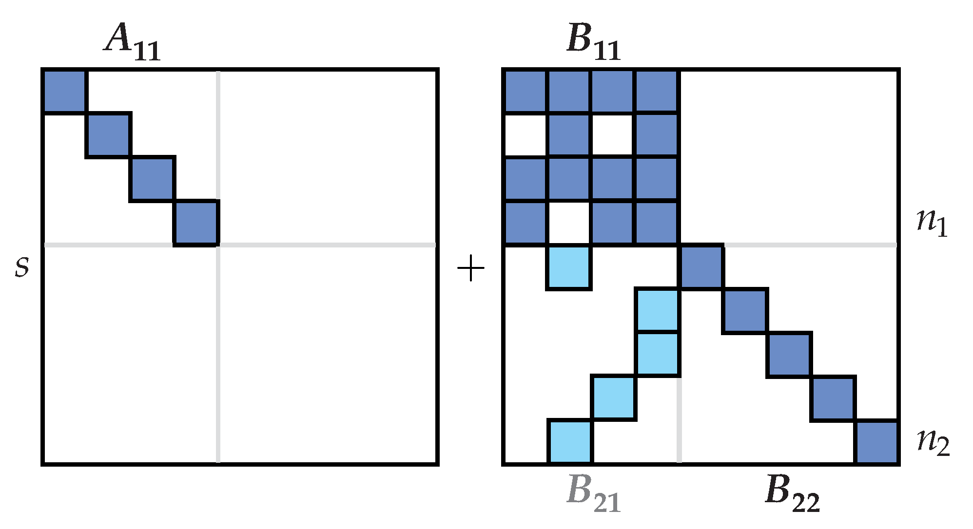
Figure 2.
Example of a dynamically degenerate circuit in which the capacitors and determining its dynamical properties create a closed loop with the voltage source E. Therefore, their voltages are not independent each other.
Figure 2.
Example of a dynamically degenerate circuit in which the capacitors and determining its dynamical properties create a closed loop with the voltage source E. Therefore, their voltages are not independent each other.
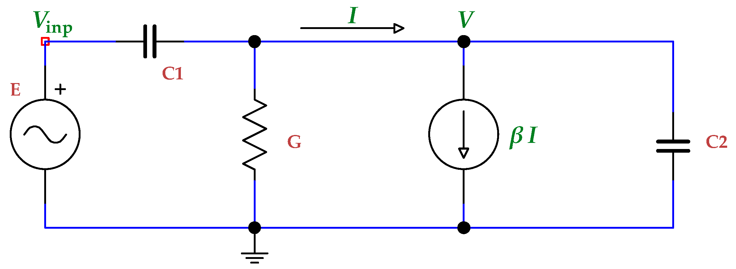
Figure 3.
The circuit diagram of the antenna low-noise preamplifier (for the multi-constellation receiver of satellite navigation). Let’s remark that the values of the passive elements were computed by a multi-objective optimization (modified goal attainment method), and for testing the frequency-scaled semisymbolic analysis, we have used the optimizer’s output that gives eight significant digits.
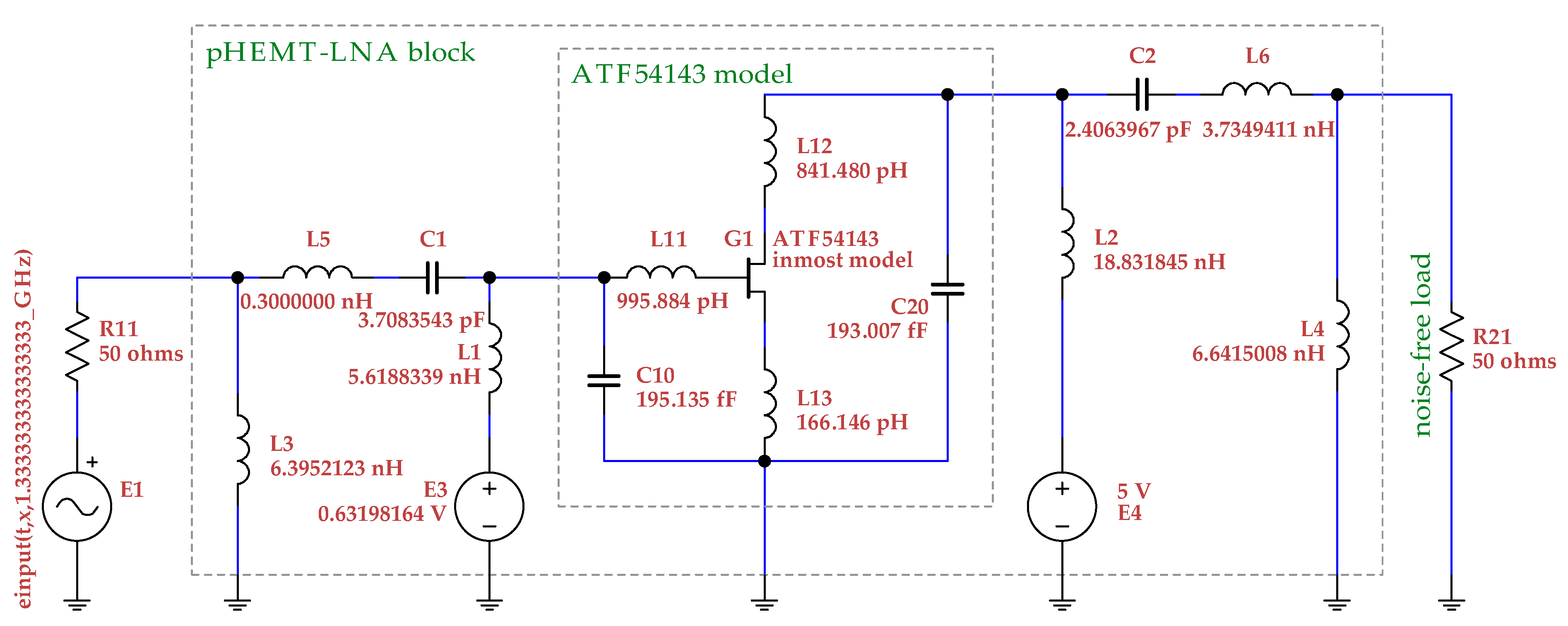
Figure 4.
The circuit diagram of the power operational amplifier. The amplifier is of an AB class, therefore, the poles and zeros of a transfer function can be determined at amplifier’s operating point.
Figure 4.
The circuit diagram of the power operational amplifier. The amplifier is of an AB class, therefore, the poles and zeros of a transfer function can be determined at amplifier’s operating point.
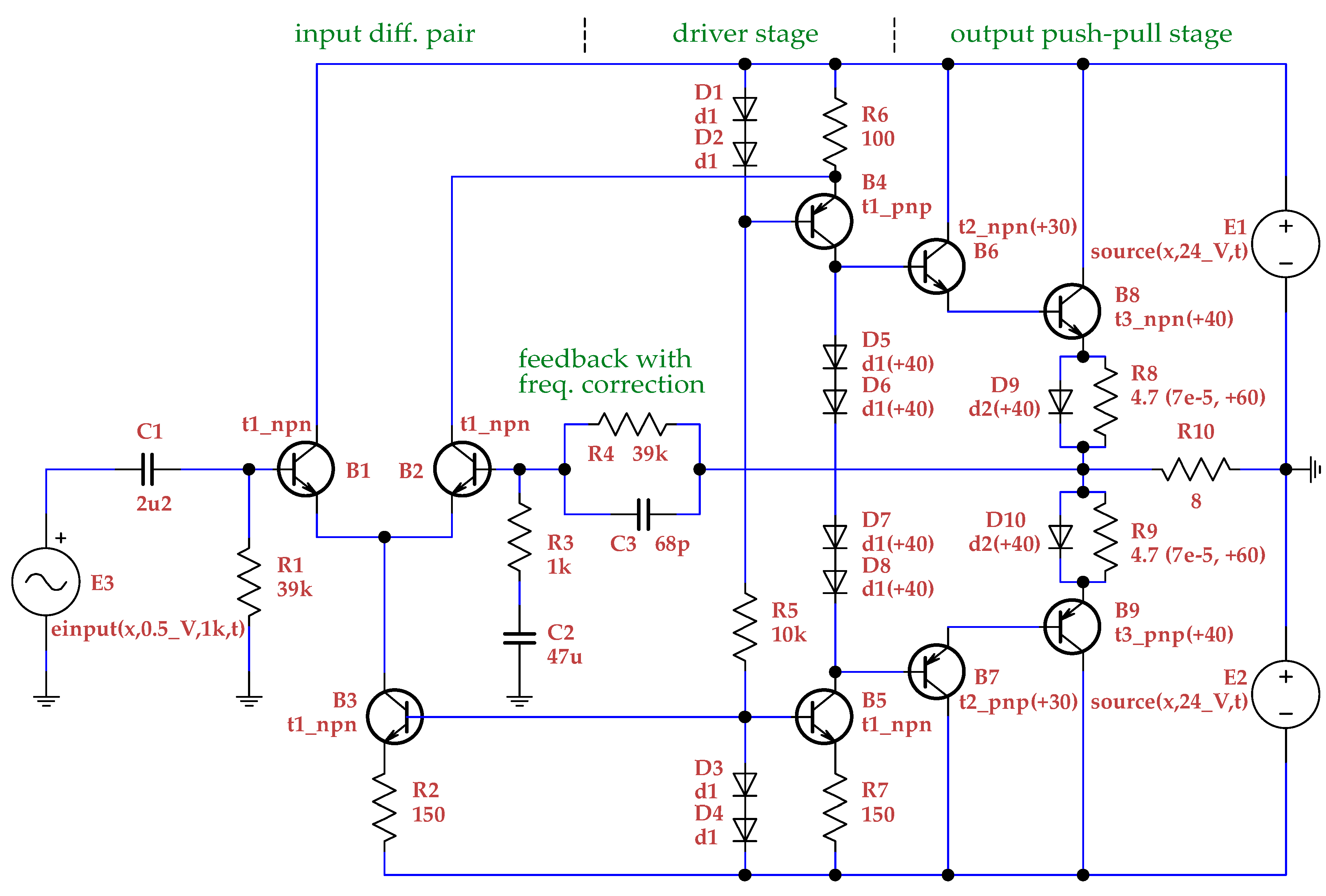
Figure 5.
The diagrams of the 272-class operational amplifier and a respective test-bench circuit. In this case, of course, it is a more difficult task due to the large number of the bipolar junction transistors and hence a large total number of small capacitances and a large size of the matrices in (1) as well.
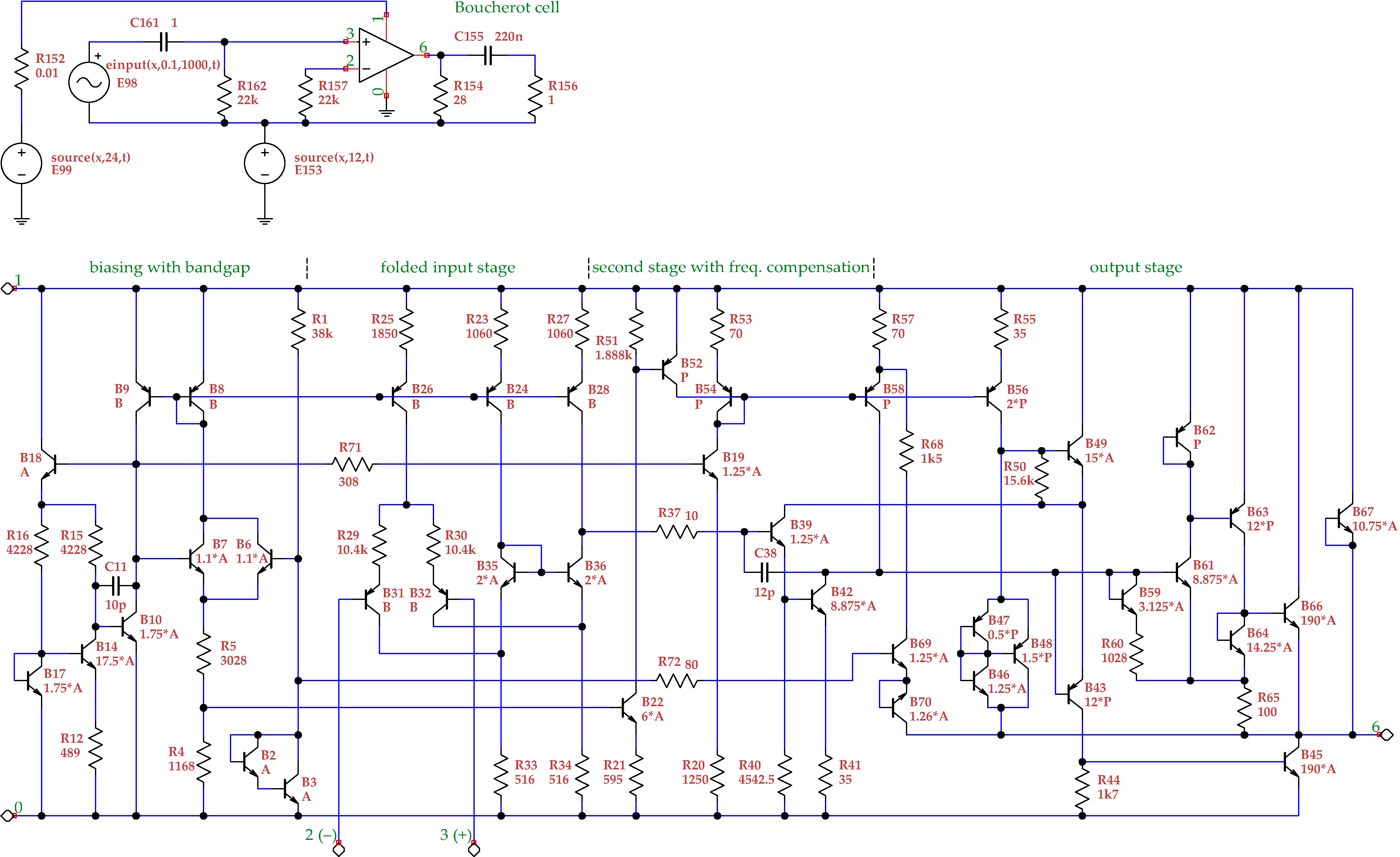
Figure 6.
The circuit diagram of the tunable microwave distributed oscillator. (Tuning can be done using the voltage sources through .) It is the most difficult task due to a number of microstrip transmission lines, because their LRCG models lead to a huge number of poles and zeros of a transfer function. Moreover, as there are many equal capacitances and inductances in these models, there exist a number of clusters of almost multiple eigenvalues (and calculating multiple eigenvalues traditionally represents a numerical problem). Although the oscillator itself is a nonlinear circuit, it is possible to calculate (especially for the weakly nonlinear oscillators like this one) so-called virtual (or pseudo) operating point, at which the circuit can be linearized and then the poles and zeros can be calculated. (And one of the so-computed poles even allows a relatively accurate estimate of oscillating frequency as shown in Table. Table 3, see footnote d!)
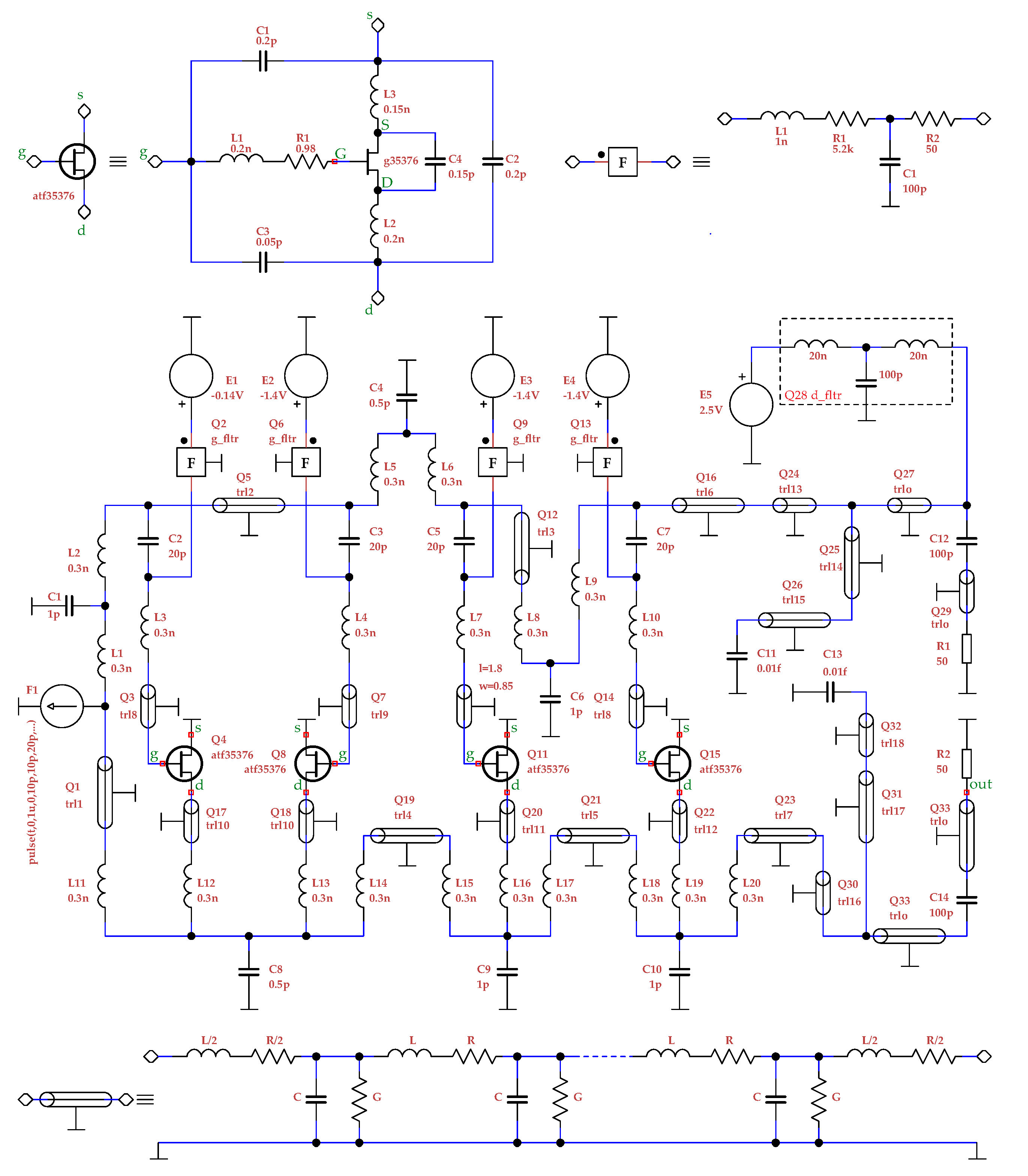

Table 1.
Differing poles and zeros of a transfer function of the AB-class power operational amplifier ( and were used for analyses with the 64-bit and 2048-bit precisions, respectively). (There were 28 poles and 28 zeros of the calculated transfer function.)
Table 1.
Differing poles and zeros of a transfer function of the AB-class power operational amplifier ( and were used for analyses with the 64-bit and 2048-bit precisions, respectively). (There were 28 poles and 28 zeros of the calculated transfer function.)
| No.a | 64-bit | 2048-bit |
|---|---|---|
| ⋯ | ⋯ | ⋯ |
| ⋯ | ⋯ | ⋯ |
| ⋯ | ⋯ | ⋯ |
| ⋯ | ⋯ | ⋯ |
a All the differing poles (upper part) and all the differing zeros (lower part) are included, they are ordered by their absolute values, and they are written in megahertz (MHz) units, e.g., the only differing pole equals approximately to GHz.
Table 2.
Differing poles and zeros of a transfer function of MDA 272 operational amplifier ( was used for both analyses). (There were 108 poles and 108 zeros.)
Table 2.
Differing poles and zeros of a transfer function of MDA 272 operational amplifier ( was used for both analyses). (There were 108 poles and 108 zeros.)
| No.a | 64-bit | 2048-bit |
|---|---|---|
| ⋯ | ⋯ | ⋯ |
| b | ||
| ⋯ | ⋯ | ⋯ |
| c | ||
| ⋯ | ⋯ | ⋯ |
| ⋯ | ⋯ | ⋯ |
| ⋯ | ⋯ | ⋯ |
| ⋯ | ⋯ | ⋯ |
| ⋯ | ⋯ | ⋯ |
| ⋯ | ⋯ | ⋯ |
| ⋯ | ⋯ | ⋯ |
| d |
a Only the most differing poles (upper part) and all differing zeros (lower part) are included, they are ordered by their absolute values, and they are written in megahertz (MHz) units, e.g., the last zero equals approximately to THz. (The differences of the zeros are more perceptible and hence they were all included.)
b This pair of complex poles is the only one with a registerable difference in the imaginary parts, although the differences are very small because . The differences detected in all other complex poles are less than one millionth, i.e., they are the same at least in the first six valid digits.
c There are only eight slightly different real poles and this one is the most different, but the difference is very small because . The differences of the other seven ones are below one millionth.
d Contrary to poles, zeros with positive real parts do not cause instability. This last zero is also the most differing, but , i.e., the difference is less than one thousandth.
Table 3.
Selected poles and a zero of the hypothetical transfer function of distributed microwave oscillator ( was used for 256-bit and 2048-bit precisions, and were also used for 64-bit precision for confirmation, and was used for 256-bit and 2048-bit & 64-bit precisions)
Table 3.
Selected poles and a zero of the hypothetical transfer function of distributed microwave oscillator ( was used for 256-bit and 2048-bit precisions, and were also used for 64-bit precision for confirmation, and was used for 256-bit and 2048-bit & 64-bit precisions)
| No.a | 256-bit | 2048-bit & 64-bit b |
|---|---|---|
| c | ||
| ⋯ | ⋯ | ⋯ |
| d | ||
| ⋯ | ⋯ | ⋯ |
| e | ||
| ⋯ | ⋯ | ⋯ |
| f | (2048-bit) | |
| (64-bit) | ||
| ⋯ | ⋯ | ⋯ |
a From a total of 266 poles, the twelve ones (1–12) with the smallest and the other twelve ones (255–266) with the biggest absolute values are included, and two other interesting couples (23,24 and 205,206) of the poles as well. Regarding zeros, only the first one (“zero at zero”) is included as an interesting test of the algorithm accuracy, the others do not have a physical sense. Again, all are written in megahertz (MHz) units, e.g., the last pole equals to around THz.
b Really, all of the poles included in the table are the same for the 2048-bit and 64-bit precisions. (Remarkable result!)
c Double (real) pole.
d This is the smallest pole with a positive real part and therefore its imaginary part can be used for an estimation of the oscillation frequency (as this circuit is “weakly nonlinear”). The presumably correct period was determined by the steady-state analysis as ns, hence the oscillation frequency should be GHz. Therefore, the errors of the estimations are only about % and % for the 256- and 2048- & 64-bit arithmetics, respectively!
e This couple of poles are physically insignificant, only included here to show the smallest poles with a difference, because all the poles 207–266 are the same for all arithmetics, which is interesting and confirms their accuracy.
f As there is a 100 pF capacitor in the path to the output, one zero of the transfer function should be at 0 Hz in principle, and it is called “zero at zero”. Only the 256-bit arithmetic was able to isolate the zero absolutely, however, both 2048-bit and 64-bit arithmetics were able to approximate it really well. This approximation can be improved by decreasing , e.g., using changes it to . However, it could be a bit risky because a too small could generate some spurious poles although quite easily recognizable.
Disclaimer/Publisher’s Note: The statements, opinions and data contained in all publications are solely those of the individual author(s) and contributor(s) and not of MDPI and/or the editor(s). MDPI and/or the editor(s) disclaim responsibility for any injury to people or property resulting from any ideas, methods, instructions or products referred to in the content. |
© 2025 by the authors. Licensee MDPI, Basel, Switzerland. This article is an open access article distributed under the terms and conditions of the Creative Commons Attribution (CC BY) license (http://creativecommons.org/licenses/by/4.0/).
Copyright: This open access article is published under a Creative Commons CC BY 4.0 license, which permit the free download, distribution, and reuse, provided that the author and preprint are cited in any reuse.


