
Submitted:
15 May 2025
Posted:
16 May 2025
You are already at the latest version
Abstract
The volume and diversity of digital information have led to a growing reliance on Machine Learning (ML) techniques, such as Natural Language Processing (NLP), for interpreting and accessing appropriate data. While vector and graph embeddings represent data for similarity tasks, current state-of-the-art pipelines lack guaranteed explainability, failing to determine similarity for given full texts accurately. These considerations can also be applied to classifiers exploiting generative language models with logical prompts, which fail to correctly distinguish between logical implication, indifference, and inconsistency, despite being explicitly trained to recognise the first two classes. We present a novel pipeline designed for hybrid explainability to address this. Our methodology combines graphs and logic to produce First-Order Logic (FOL) representations, creating machine- and human-readable representations through Montague Grammar (MG). Preliminary results indicate the effectiveness of this approach in accurately capturing full text similarity. To the best of our knowledge, this is the first approach to differentiate between implication, inconsistency, and indifference for text classification tasks. To address the limitations of existing approaches, we use three self-contained datasets annotated for the former classification task to determine the suitability of these approaches in capturing sentence structure equivalence, logical connectives, and spatiotemporal reasoning. We also use these data to compare the proposed method with language models pre-trained for detecting sentence entailment. The results show that the proposed method outperforms state-of-the-art models, indicating that natural language understanding cannot be easily generalised by training over extensive document corpora. This work offers a step toward more transparent and reliable Information Retrieval (IR) from extensive textual data.
Keywords:
verified artificial intelligence
; eXplainable AI (XAI)
; hybrid explainability
; natural language processing
; full text similarity
; spatiotemporal reasoning
1. Introduction
Factoid sentences are commonly used to characterise news [1], as they can be easily used to recognise conflicting opinions, as well as to represent the majority of a sentence type contained in Knowledge Bases (KBs) such as ConceptNet 5.5 [2] or DBpeida [3,4]. Specifically, through automated extraction, some of the concepts might not be immediately representable as nodes and edges within the KB and are often represented as full text factoid sentences, which are not easily machine-readable [5]. This is a major limitation when addressing the possibility of answering common-sense questions, as a machine cannot easily interpret the latter information, thus leading to low-accuracy results (55.9% [6]). To improve these results in the near future, we need a technique that provides a machine-readable representation of spurious text within the graph while also ensuring the correctness of the representation, going beyond the strict boundaries of a graph KB representation. We can consider this the dual problem of querying bibliographical metadata using a query language as near as possible to natural language. Notably, given the untrustworthiness of existing NLP approaches to IR, librarians still rely on domain-oriented query languages [7]. Thus, by providing a more trustworthy and verifiable representation of a full text in natural language, we can then generate a more reliable intermediate representation of the text that can be then be used to query the bibliographical data [8,9]. An adequate semantic representation of the sentences should capture both the semantic nature of the data as well as recognise implication, inconsistency, or indifference as classification outcomes over pairs of sentences. To date, this has not been considered in the literature; we have either similarity or entailment classification, but not the classification of conflicting information. At present, none of the available datasets for NLP contain such a distinction.
As the influence of Artificial Intelligence (AI) expands exponentially, so does the necessity for systems to be transparent, understandable and, above all, explainable [9]. This is further motivated by the untrustworthiness of Large Language Models (LLMs), which were not originally intended to provide reasoning mechanisms. Despite recent attempts to extend such approaches with logical guarantees [10] (Section 2.4.3), these systems are in the early stages of implementation; while they do consider a subset of the relevant logical rules of interest, they do not consider the complex logical relationships between entities within the text, limiting their application. This paper is based on current evidence in the literature, which shows that the best way to clear and detect inconsistencies within data is to provide a rule-based approach to guarantee the effectiveness of the reasoning outcome [11,12] and use logic-based systems [13,14]. Given the dualism between query and Question Answering (QA) [14], where query answering can be realised through structural similarity [15], we first address the research question on how to properly capture full text sentence similarity containing potentially conflicting and contradictory data. Then, to solidify our findings, we assess the ability of existing state-of-the-art learning-based approaches to do so, rather than solve the problem directly. Moreover, we also address the question of whether such systems can capture logical sentence meaning as well as retain spatiotemporal subtleties.
Our previous work [16] started approaching this problem. It removed the black box and began investigating the topic from the points of view of graphs and logic, which this paper continues. Explainability is vital to ensuring users’ trust in sentence similarity. The Logical, Structural and Semantic text Interpretation (LaSSI) (https://github.com/LogDS/LaSSI/releases/tag/v2.1, Accessed on 14 May 2025) pipeline takes a given full text and transforms it into First-Order Logic (FOL), returning a representation that is both human- and machine-readable. It provides a way for similarity to be determined from full texts, as well as a way for individuals to reverse engineer how this similarity was calculated. Graphs are generated as intermediate representations from dependency parsing: given sentences with equivalent meaning that produce structurally disparate graphs, we obtain equality formulae. Overall sentence similarity is then derived by reconciling such formulae with minimal propositions. By providing a tabular representation of both sentences, we can derive the confidence associated with the two original sentences, naturally leading to a non-symmetric similarity metric considering the possible worlds where these sentences are valid.
This paper addresses the following research questions through both theoretical and experiment-driven results, where the latter are supported by a dataset available online (https://osf.io/g5k9q/, Accessed on 14 May 2025):
- RQ №1
- Can sentence transformers’ embeddings and graph-based solutions correctly capture the notion of sentence entailment? Theoretical results (Section 4.1) indicate that similarity metrics that mainly consider the symmetric properties of the data are unsuitable for capturing the notion of logical entailment, for which we at least need quasi-metric spaces or divergence measures. This paper offers the well-known metric of confidence [17] for this purpose and contextualises it within logic-based semantics for full texts.
- RQ №2
-
Can pre-trained language models correctly capture the notion of sentence similarity? The previous result should imply the impossibility of accurately deriving the notion of equivalence, as entailment implies equivalence through if-and-only-if relationships but not vice versa. Meanwhile, the notion of sentence indifference should be kept distinct from the notion of conflict. We designed empirical experiments with certain datasets to address the following sub-questions:
- (a)
- Can pre-trained language models capture logical connectives? Current experiments (Section 4.2.1) show that pre-trained language models cannot adequately capture the information contained in logical connectives. The results can be improved after elevating such connectives as first-class citizens (Simple Graphs (SGs) vs. Logical Graphs (LGs)). Furthermore, given the experiments’ outcomes, vector embedding likely favours entities’ positions in the text and discards logical connectives within the text as stop words.
- (b)
- Can pre-trained language models distinguish between active and passive sentences? Preliminary experiments (Section 4.2.2) show that structure alone is insufficient for implicitly deriving semantic information. Additional disambiguation processing is required to derive the correct representation desiderata (SGs and LGs vs. logical). Furthermore, pre-trained language models that either mask and tokenise the sentence or exploit Abstract Meaning Representation (AMR) representation fail to faithfully represent simple sentence structures, even without calling on logical inference or negation detection.
- (c)
- Can pre-trained language models correctly capture the notion of logical implication, e.g., in spatiotemporal reasoning? Spatiotemporal reasoning requires specific part-of and is-a reasoning. This, to the best of our knowledge and at the time of this paper’s writing, is unprecedented in the existing literature on logic-based text interpretation. Consequently, we argue that these notions cannot be captured with embeddings alone or with graph-based representations using merely structural information, as this requires categorising the logical function of each entity within the text as well as correctly addressing the interpretation of the logical connectives occurring (Section 4.2.3).
- RQ №3
- Is our proposed technique scalable? Benchmarks over a set of 200 sentences retrieved from sentences within ConceptNet [2] (Section 4.3) indicate that our pipeline runs in at most linear time over the number of sentences, thus indicating the optimality of the envisioned approach.
- RQ №4
- Can a single rewriting grammar and algorithm capture most factoid sentences? Our Discussion (Section 5) remarks that this preliminary work improves over the sentence representation from our previous solution, but there are still ways to improve the current pipeline. We also argue the following: given that training-based systems also use annotated data to correctly identify patterns and return correct results (Section 2.2), the output provided by training-based algorithms, without abductive reasoning [18,19] or relational learning support [20], can only be as correct as a human’s ability to consider all possible cases for validation. Furthermore, to better ensure the correctness of the inference process, the inverse approach should be investigated, which is commonly used in Upper Ontologies [21] through machine teaching [22,23,24].
This paper primarily extends our previous implementation as follows:
- We extend our logical representation of sentences to also consider existential quantifiers (subject ellipsis): this is paired with an algorithmic extension of our pipeline (Appendix B.3.1).
- We capture richer sentence semantics by acknowledging the logical functions of adverbial phrases rather than just recognising the type associated with this (Section 3.2.3) and, for the first time, provide a pipeline enabling logical sentence analysis of the sentence per Italian Linguistics (Section 2.3.1).
- We capture the notion of semantic entailment across atoms through the Parmenides KB (Appendix D.2.1).
- The ad hoc phase (Section 3.2) now addresses some of the errors generated through automated Universal Dependency (UDs) extraction by leveraging limited syntactical context and annotated dictionaries from the a priori phase (Supplement III and Supplement IV).
- We extend our pipeline to plot an explanation for the implication, inconsistency, or indifference for each pair of sentences (Section 5.3).
The remainder of this paper is structured as follows: After contextualising our attempt of introducing, for the first time, verified AI within the context of NLP through explainability (Section 2.1), we mainly address current NLP concepts for conciseness purposes (Section 2.2). Then, we prove that our pipeline achieves hybrid explainability by showing its ability to provide a priori explanations (Section 3.1), where the text is enriched with contextual and semantic information, ad hoc explanations (Section 3.2), through which the sentence is transformed into a verifiable representation (be that a vector, a graph, or a logical formula), and a final human-understandable ex post (Section 3.3), through which we distil the desired textual representation generated by the forthcoming phase into a similarity matrix. This helps to better appreciate how the machine can interpret the similarity of the text. After providing an in-depth discussion on the improvements over our previous work (Section 5.1), we provide a pipeline ablation study (Section 5.2) and compare our explainers to other textual explainers (SHAP and LIME) using state-of-the-art methodologies to tokenised text and correlate it with the predicted class (Section 5.3). Last, we draw our conclusions and indicate some future research directions (Section 6).
2. Related Works
2.1. General Explainable and Verified Artificial Intelligence (GEVAI)
A recent survey by Seshia et al. introduced the notion of verified AI [25], through which we seek greater control by exploiting reliable and safe approaches to derive a specification describing abstract properties of the data . Through verifiability, the specification itself can be used as a witness of the correctness of the proposed approach by determining whether the data satisfy such specification, i.e., (formal verification). This survey also revealed that, at the time of its writing, providing a truly verifiable approach of NLP is still an open challenge, remaining unresolved with current techniques. In fact, specification is not simply considered the outcome of a classification model or the result of applying a traditional explainer, but rather a compact representation of the data in terms of the properties it satisfies in a machine- and human-understandable form. Furthermore, as remarked in our recent survey [26], the possibility of explaining the decision-making process in detail, even in the learning phase, goes hand in hand with using an abstract and logical representation of the data. However, if one wants to use a numerical approach to represent the data, such as when using Neural Networks (NNs) and producing sentence embeddings from transformers (Section 2.4), then one is forced to reduce the explanation of the entire learning process to the choice of weights useful for minimising the loss function and to the loss function itself [27]. A possible way to partially overcome this limitation is to jointly train a classifier with an explainer [28], which might then pinpoint the specific data features leading to the classification outcome [29]: as current explainers mainly state how a single feature affects the classification outcome, they mainly lose information on the correlations between these features, which are extremely relevant in NLP (semantic) classification tasks.
More recent approaches [9] have attempted to revive previous non-training-based approaches, showing the possibility of representing a full sentence with a query out mainly via semantic parsing [8]. A more recent approach also enables sentence representation in logical format rather than ensuring an SQL representation of the text. As a result, the latter can also be easily rewritten and used for inference purposes. Notwithstanding the former, researchers have not covered all the rewriting steps required to capture different linguistic functions and categorise their role within the sentence, unlike in this study. Furthermore, while the authors of [9] attempted to answer questions, our study takes a preliminary step back. We first test the suitability of our proposed approach to derive correct sentence similarity from the logical representation. Then, we then tackle the possibility of using logic-based representations to answer questions and ensure the correct capturing of multi-word entities within the text while differentiating between the main entities based on the properties specifying them.
Our latest work also remarks the possibility of achieving verification when combined with explainability in a way that makes the data understandable to both humans and machines [26]. This identifies three distinct phases to be considered as prerequisites for achieving good explanations: First, within the first a propri explanation, unstructured data should achieve a higher structural representation level by deriving additional contextual information from the data and environment. Second, the ad hoc explanation should provide an explainable way through which a specification is extracted from the data, where provenance mechanisms help trace all the data processing steps. If represented as a logical program, the specification can also ensure both human and machine understandability by being represented in an unambiguous format. Lastly, the ex post phase (post hoc in [28]) should further refine the previously generated specifications by achieving better and more fine-grained explainability. Therefore, we can derive even more accessible results and ease the comparisons between models while enabling their comparison with other data. Our Section 3 reflects these phases.
2.2. Natural Language Processing (NLP)
Part of Speech (POS) tagging algorithms work as follows: each word in a text (corpus) is marked up as belonging to a specific part of speech based on the term’s definition and context [30]. Words can be then categorised as nouns, verbs, adjectives, or adverbs. In Italian linguistics (Section 2.3.1), this phase is referred to as the grammatical analysis of a sentence structure and is one the most fine-grained analyses. As an example for POS tags, we can retrieve these initial annotations for the sentence “Alice plays football” from Stanford CoreNLP [31], identifying “Alice” as a proper noun (NNP), “plays” as a verb (VBZ—present tense, third-person singular), and “football” as a noun (NN) and thus determining the subject–verb–object relationship between these words.
Dependency parsing [32] refers to the extraction of language-independent grammatical functions expressed through a minimal set of binary relationships connecting POS components within the text, thus allowing a semistructured, graph-based representation of the text. These dependencies are beneficial in inferring how one word might relate to another. We can also extract these UDs through Stanford CoreNLP, whereby we obtain annotations for each word in the sentence, giving us relationships and types. For example, a conj [33] dependency represents a conjunct, which is a relation between two elements connected by a cc [34] (a coordination determining what type of group these elements should be in).
As shown in Figure 1b and Figure 1d, relationships are labelled on the edges, and types are labelled underneath each word. Looking at Figure 1d, Newcastle and traffic are all children of have, through nsubj and dobj relationships, respectively. Types are determined from POS tags [32], so we can identify that have is a verb as it is annotated with VBP (a verb of the present tense and not third-person singular). The nsubj relation stands for the nominal subject, and dobj is the direct object, meaning that Newcastle acts upon traffic by having traffic. Brighton is also a child of Newcastle through a conj relation, and Newcastle has a cc relation with and, implying that these two subjects are related. Consequently, if we know Newcastle has traffic, then it holds that Brighton does as well. These POS tags also indicate Newcastle and Brighton are proper nouns as they both have NNP types.
Abstract Meaning Representation (AMR) graphs proposed by Goodman et al. [36] provide a straightforward sentence representation as graphs, which mainly connects the sentence verb to the arguments belonging to the sentence. Although this representation can be enhanced to support full Multi-Word Entity Resolution using background knowledge (wiki relationship in Figure 1a, missing from Figure 1b), and despite its recent application in LLMs for achieving logical reasoning abilities [10], this representation discards relevant semantic relationships between words in the text, which might be relevant to faithfully capturing the distinction between subjects, (direct) objects, and other adverbial phrases occurring within the sentence. In comparing Figure 1c with Figure 1d, it is clear that specific propositions such as “in”, useful for extracting information concerning a space-related adverbial phrase, are discarded from the AMR graph but retained in the UDs graph. Furthermore, both the subject of the main sentence (“traffic”) and the space-related adverbial phrase are marked with the same relationship label ARG1, while UDs graphs distinguish these two logical functions with two distinct relationships, nsubj and nmod. For this reason, our approach uses UDs rather than AMR for retaining complex semantic representations of sentences. To overcome UDs’s only shortcoming, we provide a preliminary a priori explanation phase, enabling multi-word entity recognition using well-known NLP tools and vocabularies (Section 3.1).
Capturing syntactical features through training is challenging. NN-based approaches are not proficient in precisely capturing relationships within text, as they fall down the same limitations as vector-based representations of sentences. Figure 1d shows how AI struggles with understanding negation from full text: the sentence was fed into a natural language parser [37], and the result shows no sign of a negated (neg) dependency, despite “but not” being contained within the sentence. Still, we can easily identify and fix these issues before returning the Dependency Graph (DG) to our LaSSI pipeline.
2.3. Linguistics and Grammatical Structure
The notion of the systematic and rule-based characterisation of human languages pre-dates modern studies on language and grammar: Aṣṭādhyāyī by Pāṇini utilised a derivational approach to explain the Sanskrit language, where speech is generated from theoretical, abstract statements created by adding affixes to bases under specific conditions [38]. This further supports the idea of representing most human languages in terms of grammatical derivational rules, from which we can identify the grammatical structure and functions of the terms occurring in a piece of text [39]. This induces the recursive structure of most Indo-European languages, including English, which should be addressed to better analyse the overall sentence structure into its minimal components.
Consider the example in Figure 2; this could continue infinitely as a consequence of recursion in language due to the lack of an upper bound on grammatical sentence length [40]. As the full text can be injected with semantic annotations, these can be further leveraged to derive a logical representation of the sentence [9].
Richard Montague developed a formal approach to natural language semantics, which later became known as Montague Grammar (MG), where natural and formal languages can be treated equally [42] to allow for the rewriting of a sentence in a logical format by assuming the possibility of POS tagging. MG assumes languages can be rewritten given their grammar [43], preserving logical connectives and expressing verbs as logical predicates. MG then provides a set of rules for translating this into a logical form; for instance, a sentence (S) can be formed by combining a noun phrase () and a verb phrase (). We can also find the meaning of a sentence obtained by the rule , whereby the function for is applied to the function . MG uses a system of types to define different kinds of expressions and their meanings. Some common types include t, denoting a term (a reference to an entity), and f, denoting a formula (a statement that can be true or false). The meaning of an expression is obtained as a function of its components, either by applying the function or by constructing a new function from the functions associated with the component. This compositionality makes it possible to assign meanings reliably to arbitrarily complex sentence structures, enabling us to then extract predicate logic from this, so the sentence “Alice plays football” becomes play(Alice, football).
However, MG only focuses on the logical form of full text, overlooking the nuances of context and real-world knowledge. For example, does “Newcastle” refer to “Newcastle-upon-Tyne, United Kingdom”, “Newcastle-under-Lyme, United Kingdom”, “Newcastle, Australia”, or “Newcastle, Northern Ireland”? Without an external KB or ontology, it is difficult to determine which of these it could be unless the full text provides relevant explicit information. Therefore, providing a dictionary of possible matches for all words in the sentence can significantly improve the Multi-Word Entity Unit (MEU) recognition, meaning known places, people, and organisations can be matched to enhance the understanding of the syntactic structure of a given full text. At the time of this paper’s writing, no Graph Query Language (GQL) can combine semantic utilities related to entity resolution alongside structural sentence rewriting. Therefore, this forces us to address minimal sentence rewriting through GQLs, while considering the main semantic-driven rewritings in our given Python code base, where all of these are accounted for.
2.3.1. Italian Linguistics
Not all grammatical information can be captured from MG alone: we can identify words that are verbs and pronouns, but these can both be broken down into several sub-categories that infer different rewriting that is not necessarily apparent from the initial structure of the sentence. For instance, a transitive verb is a verb that can take a direct object, “the cateats the mouse”, so when rewriting into the logical form, we know that a direct object must exist: eat(cat, mouse), where eat is acting on the mouse. However, if the verb is intransitive, “going across the street”, then the logical form must not have a direct object and is thus removed, as the target does not reflect the direct object. Therefore, this sentence becomes go(?)[(SPACE:street[(det:the), (type:motion through place)])], as go does not produce an action on the street. The target is removed from the rewriting to reflect the nature of intransitive verbs. All these considerations are not accounted for in current NLP pipelines for QA [9], where merely simple binary relationships are accounted for, and the logical function of the POS components is not considered.
In Italian linguistics, the examination of a proposition, commonly referred to as logical analysis, is the recognition process for the components of a proposition and their logical function within the proposition itself [44]. In this regard, this analysis recognises each clause/sentence as a predicate with its (potentially passive) subject, where we aim to determine the function of every single component: the verb, the direct object, and any other “indirect complement” that can refer to either an indirect object, adverbial phrase, or a locative [45]. This kind of analysis aims to determine the type of purpose the text is communicating and characterises each adverbial phase based on the information conveyed (e.g., limitation, manner, time, space) [44]. This significantly differs from the POS tagging of each word appearing in a sentence, through which each word is associated to a specific POS (adjective, noun, verb), as more than just one single word could participate in providing the same description. Concerning Figure 1b, both Newcastle and Brighton are considered part of the same subject, Newcastle and Brighton, while in Newcastle is recognised as a space adverbial of time stay in place given that the preposition it and the verb is are not indicating a motion rather than a state. Concerning Figure 1d, this analysis considers “but not in the city centre” (Figure 1d) a separate coordinate clause, where “There is (not) traffic” is subsumed from the main sentence. We argue that the possibility of further extracting more contextual knowledge from a sentence via logical analysis tagging helps the machine to categorise the text’s function better, thus providing both machine- and human-readable explanations. Although there is no support in the English language literature for these sentence-linguistic functions, since such functions are almost standard in all Indo-European languages, they can naturally be defined for the English language. In support of this, Table 1 showcases the rendition of such functions and, given the lack of such characterisation in English, we freely exploit the characterisation found in Italian linguistics and contextualise this for the English language.
To distinguish between Italian and English linguistic terminology, we refer to the characterisation of such sentence elements beyond the subject–verb–direct object characterisation as logical functions. Section 3.2.3 provides additional information on how such linguistic functions are recognised from a rewritten intermediate graph representation within LaSSI for the English language. We define such linguistic functions and how they can be matched through rewriting rules expressed within our ontology, Parmenides.
2.4. Pre-Trained Language Models
We now introduce our competing approaches, which all work by assuming that information can be distilled from a large set of annotated documents and is suitable training tasks, leading to a model representation minimising the loss function over an additional training dataset. We focus on pre-trained language models for sentence similarity and logical prediction tasks. Table 2 summarises our findings.
2.4.1. Sentence Transformers
Google first introduced transformers [50] as a compact way to encode semantic representations of data into numerical vectors, usually within a Euclidean space, through a preliminary tokenisation process. After converting tokens and their positions into vector representations, a final transformation layer provides the final vector representation for the entire sentence. The overall architecture seeks to learn a vector representation for an entire sentence, maximising the probability distribution over the extracted tokens. This is ultimately achieved through a loss minimisation task that depends on the transformer’s architecture of choice; while masking considers predicting the masked out tokens by learning a conditional probability distribution over the non-masked one, autoregression learns a stationary distribution for the first token and a conditional probability distribution aiming to predict the subsequent tokens, which are gradually unmasked. While sentence transformers usually adopt the former approach, generative LLMs (discussed in Section 2.4.3) use the latter.
Pre-trained sentence transformer models are extensively employed to turn text into vectors known as embeddings and are fine-tuned on many datasets for general-purpose tasks such as semantic search, grouping, and retrieval. Nanjing University of Science and Technology and Microsoft Research jointly created MPNet [46], which aims to consider the dependency among predicted tokens through permuted language modelling while considering their position within the input sentence. RoBERTa [47], a collaborative effort between the University of Washington and Facebook AI, is an improvement over traditional BERT models, where masking only occurs at data pre-processing, by performing dynamic masking, thus generating a masking pattern every time a training token sequence is fed to the model. The authors also recognised the positive effect of hyperparameter tuning over the resulting model, thus systematising the training phase while considering additional documents. Lastly, Microsoft Research [48] took an opposite direction on the hyperparameter tuning challenge: rather than consider hundreds of millions of parameters, MiniLMv2 considers a simpler approach compressing large transformers via pre-trained models, where a small student model is trained to mimic the pre-trained one. Furthermore, the authors exploited a contrastive learning objective for maximising the sentence semantics’ similarity mapping: given a training dataset composed of pairs of full text sentences, the prediction task is to match one sentence from the pair, and then the other is given.
Recent surveys on the expressive power of transformer-based approaches, mainly for capturing text semantics, reveal some limitations in their reasoning capabilities. First, when two sentences are unrelated, the attention mechanisms are dominated by the last output vector [28], which might easily lead to hallucination and untrustworthy results such as the ones due by semantic leakage [51]. Second, theoretical results have suggested that these approaches are unable to reason on propositional calculus [52]. If the impossibility of simple logical reasoning during the learning phase is confirmed, this would strongly undermine the possibility of relying on the resulting vector representation for determining complex sentence similarity. Lastly, while these approaches’ ability to represent synonymy relations and carry out multi-word name recognition is recognised, their ability to discard parts of the text deemed irrelevant is well known to result in some difficulty with capturing higher-level knowledge structures [28]. That said, if a word is then considered a stop word, it will not be used in the similarity learning mechanism, and the semantic information will be permanently lost. On the contrary, a learning approach exploiting either AMR and UD graphs can potentially limit this information loss. Section 2.4.3 discusses more powerful generative-based approaches that attempt to overcome the limitations above.
2.4.2. Neural IR
IR concerns retrieving full text documents given a full text query. Classical approaches tokenise the query into several words of interest, which are then used to retrieve the documents within a corpus. Each document is then ranked according to the presence of each token in the document within the corpus [53]. Neural IR improved over classical IR, which was originally heavily text-bound without considering the semantic information of the text. After representing each query and document as a vector, the relevance of the document with respect to the given query is computed through the vector dot product. While the first version for these approaches exploited transformers similarly to those in the previous section, where documents and queries are represented as one single vector, late interaction approaches such as ColBERTv2, proposed by Keshav et al. [49], provide a finer granularity representation by encoding the former into a multi-vector representation. After finding each document token maximising the dot product with a given query token, the final document ranking score is defined by summing all the maximising dot products. Training is then performed to maximise the matches of the given queries with human-annotated documents, marked as positive or negative matches for each query. Please observe that although this approach might help maximise the recall of the documents based on their semantic similarity to the query, the query tokenisation phase might lose information concerning the correlation between the different tokens occurring within the document, thus potentially disrupting any structural information occurring across query tokens. On the other hand, retaining semantic information concerning the relationships between entities leads us to a better logical and semantic representation of the text, as our proposed approach proves.
This paper considers benchmarks against ColBERTv2 through the pre-trained RAGatouille v0.0.9 (https://github.com/AnswerDotAI/RAGatouille, Accessed on 22 April 2025) library.
2.4.3. Generative Large Language Models (LLMs)
As a result of the autoregressive tasks generally adopted by generative LLM models, when the system is asked about concepts on which it was not trained initially, it tends to invent misleading information [54]. This is inherently due to the probabilistic reasoning embedded within the model [55], not accounting for inherent semantic contradiction implicitly resulting from the data through explicit rule-based approaches [14,56]. These models do not account for probabilistic reasoning by contradiction, with facts given as conjunctions of elements, leading to the inference of unlikely facts [57,58]. All these consequences are self-evident in current state-of-the-art reasoning mechanisms. They are currently referred to as hallucinations, which cannot be trusted to verify the inference outcome [59].
DeBERTaV2+AMR-LDA, proposed by Qiming Bao et al. [10], is a state-of-the-art model supporting sentence classification through logical reasoning using a generative LLM. The model can conclude whether the first given sentence entails the second or not, thus attempting to overcome the above limitations of LLM. After deriving an AMR representation of a full text sentence, the graphs are rewritten to obtain logically equivalent sentence representations for equivalent sentences. AMR-LDA is used to augment the input prompt before feeding it into the model, where prompts are given for logical rules of interest to classify the notion of logical entailment throughout the text. Contrastive learning is then used to identify logical implications by learning a distance measure between different sentence representations, aiming to minimise the distance between logically entailing sentences while maximising the distance between the given sentence and the negative example. This approach has several limitations: First, the authors only considered equivalence rules that frequently occur in the text and not all of the possible equivalence rules, thus heavily limiting the reasoning capabilities of the model. Second, in doing so, the model does not exploit contextual information from the knowledge graphs to consider part-of and is-a relationships relevant for deriving correct entailment implications within spatiotemporal reasoning. Third, due to the lack of paraconsistent reasoning, the model cannot clearly distinguish whether the missing entailment is due to inconsistency or whether the given facts are not correlated. Lastly, the choice of using AMR heavily impacts the ability of the model to correctly distinguish different logical functions of the sentence within the text.
The present study overcomes the limitations above in the following manner: First, we avoid hardcoding all possible logical equivalence rules by interpreting each formula using classical Boolean-valued semantics for each atom within the sentences. After generating a truth table with all the atoms, we then evaluate the Boolean-valued semantics for each atom combination (Appendix D.1). In doing so, we avoid the explosion problem by reasoning paraconsistently, thus removing the conflicting worlds (also Appendix D.1). Second, we introduce a new compact logical representation, where entities within the text are represented as functions (Section 3.2.4); the logical entailment of the atoms within the logical representation is then supported by a knowledge base expressing complex part-of and is-a relationships (Appendix D.2). Third, we consider a three-fold classification score through the confidence score (Definition 6): while and can be used to differentiate between implication and inconsistency, intermediate values will capture indifference. Lastly, we use UD graphs rather than AMR graphs (Supplement I.1), similarly to recent attempts at providing reliable rule-based QA [9].
This study considered benchmarking against the pre-trained LLM classifier, which was made available through HuggingFace by the original paper’s authors (AMR-LE-DeBERTa-V2-XXLarge-Contraposition-Double-Negation-Implication-Commutative-Pos-Neg-1-3).
3. Materials and Methods
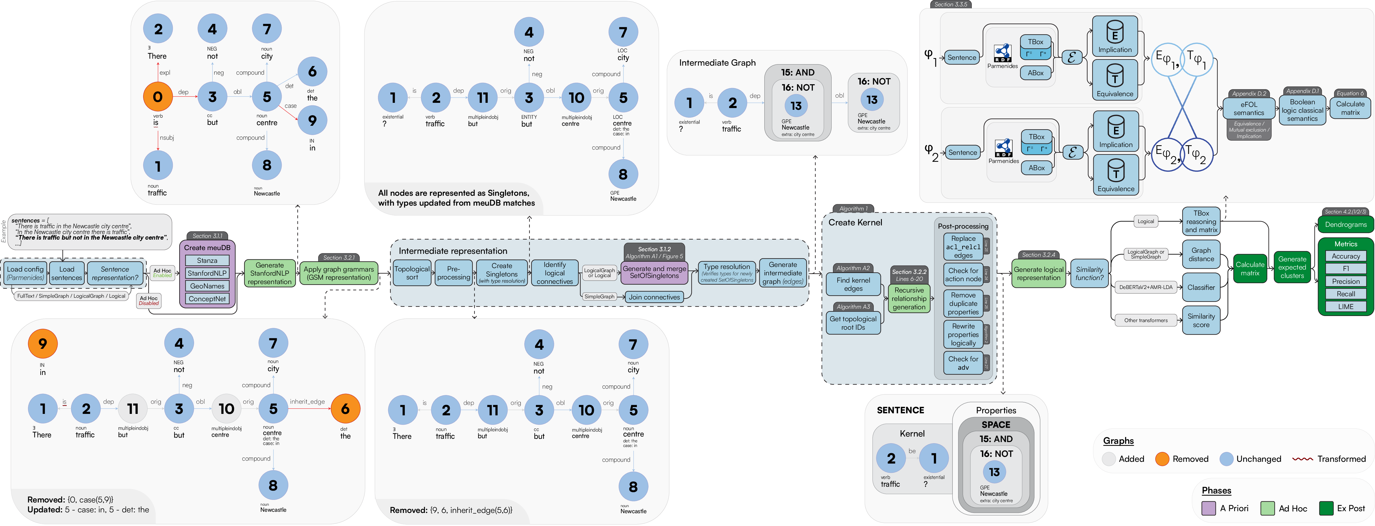
Let α and β be full text sentences. In this paper, we consider only factoid sentences that can at most represent existentials, expressing the omission of knowledge to, at some point, be injected with new, relevant information. τ represents a transformation function, in which the vector and logical representations are denoted as and for α and β, respectively. From τ, we want to derive a logical interpretation through φ while capturing the common-sense notions from the text. We then need a binary function that expresses this for each transformation τ (Section 4.1). Figure 4 offers a birds-eye view of the entire pipeline as narrated in the present paper.
Figure 3 details the former by adding references to specific parts of the paper while providing a running example.
Figure 3.
Detailed view of Figure 4: The pipeline shows a running example of the sentence #2 from RQ №2(c), “There is traffic but not in the Newcastle city centre”: graphs provide the representation returned by specific pipeline tasks, where colours highlight the performed changes. We retain colours from Figure 4 for linking across the same tasks. Due to page limitations, we refer to Figure 5 for a detailed description of the transformation needed to generate an Intermediate Graph after identifying the logical connectives. We also refer to Sentence 2 occurring in Figure 22 for a graphical representation of both the final logical representation of the sentence (Section 3.2.4) as well as a high-level representation of the reasoning process (Section 3.3.5)
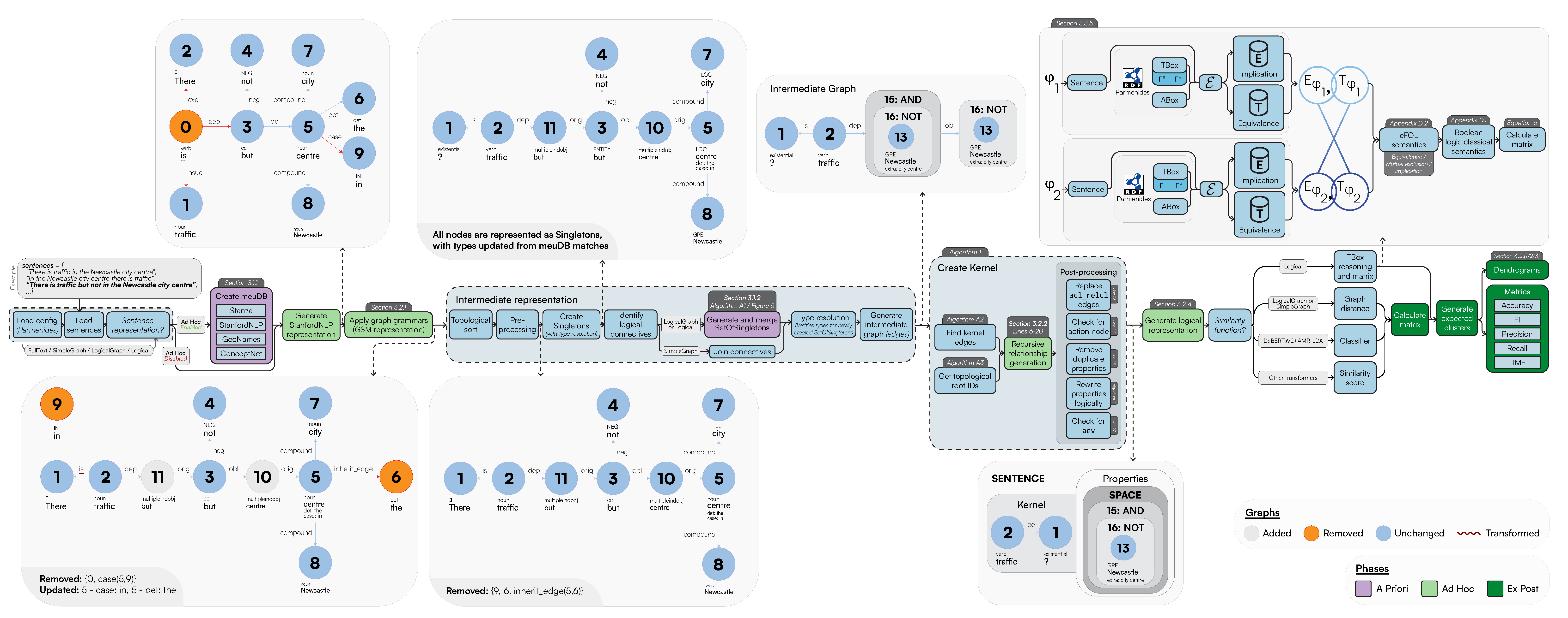
Figure 4.
LaSSI Pipeline: Operational description of the pipeline, reflecting the outline of this section.
Figure 4.
LaSSI Pipeline: Operational description of the pipeline, reflecting the outline of this section.
3.1. A Priori
In the a priori explanation phase, we aim to enrich the semantic information for each word (Section 3.1.1) to subsequently recognise multi-word entities (Section 3.1.2) with extra information (i.e., specifications, Appendix A.2.1) by leveraging the former. This information will be used to pair the intermediate syntactic and morphological sentence representation achieved through subsequent graph rewritings (Section 3.2) with the semantic interpretation derived from the phase narrated within the forthcoming subsections.
The main data structure used to nest dependent clauses represented as relationships occurring at any recursive sentence level is the Singleton. This is a curated class used throughout the pipeline to portray entities within the graph from the given full text. This also represents the atomic representation of an entity (Section 3.1.1); it includes each word of a multi-word entity (Section 3.1.2) and is defined with the following attributes: id, named_entity, properties, min, max, type, confidence, and kernel. When kernel is none, properties mainly refer to the entities, thus including the aforementioned specifications (Appendix A.2.1); otherwise, they refer to additional entities leading to logical functions associated with the sentence. Kernel is used when we want to represent an entire sentence as a coarser-grained component of our pipeline: this is defined as a relationship between a source and target mediated by an edge label (representing a verb), while an extra Boolean attribute reflects its negation (Section 3.2.2). The source and target are also Singletons as we want to be able to use a kernel as a source or target of another kernel (e.g., to express causality relationships) so that we have consistent data structures across all entities at all stages of the rewriting. The properties of the kernel could include spatiotemporal or other additional information, represented as a dictionary, which is used later to derive logical functions through logical sentence analysis (Section 3.2.3).
3.1.1. Syntactic Analysis using Stanford CoreNLP
This step aims to extract syntactic information from the input sentences and using Stanford CoreNLP. A Java service within our LaSSI pipeline utilises Stanford CoreNLP to process the full text, generating annotations for each word. These annotations include base forms (lemmas), POS tags, and morphological features, providing a foundational understanding of the sentence structure while considering entity recognition.
The Multi-Word Entity Unit DataBase (meuDB) contains information about all variations of each word in a given full text. This could refer to American and British spellings of a word like “centre” and “center”, or typos in a word like “interne” instead of “internet”. Each entry in the meuDB represents an entity match appearing within the full text, with some collected from specific sources, including GeoNames [60] for geographical places, SUTime [61] for recognising temporal entities, Stanza [62] and our curated Parmenides ontology for detecting entity types, and ConceptNet [63] for generic real-world entities. Depending on the trustworthiness of each source, we also associate a confidence weight: for example, as the GeoNames gazetteer contains noisy entity information [60], we multiply the entity match uncertainty by 0.8 as determined in our previous research [16]. Each match also carries the following additional information:
- start and end characters respective to their character position within the sentence: these constitute provenance information that is also pertained in the ad hoc explanation phase (Section 3.2), thus allowing the enrichment of purely syntactic sentence information with a more semantic one.
- text value referring to the original matched text.
-
monad for the possible replacement value:
- -
- Supplement III.3 details that this might eventually replace words in the logical rewriting stage.
Changes were made to the MEU matching to improve its efficiency in recognising all possibilities of a given entity. In our previous solution, only the original text was used. Now, we perform a fuzzy match through PostgreSQL for lemmatised versions of given words [64] rather than through Python code directly to boost the recognition of multi-word entities by assembling other single-word entities. Furthermore, when generating the resolution for MEUs, a typed match is also performed when no match is initially found from Stanford NLP, so the type from the meuDB is returned for the given MEU.
This categorisation subsequently allows the representation of each single named entity occurring in the text to be represented as a Singleton as discussed before.
3.1.2. Generation of SetOfSingletons
A SetOfSingletons is a specific type of Singleton containing multiple entities, an array of Singletons. As showcased by Figure 5, a group of items is generated by coalescing distinct entities grouped into clusters as indicated by UDs relationships, such as the coordination of several other entities or sentences (conj), the identification of multi-word entities (compound), or the identification of multiple logical functions attributed to the same sentence (multipleindobj, derived after the Generalised Graph Grammar (GGG) rewriting of the original UDs graph). Each SetOfSingletons can be associated with types.
Figure 5.
Continuing the example from Figure 3, we show how different types of SetOfSingletons generated from distinct UD relationships leading to the generation of an Intermediate Graphs. We showcase coordination (e.g., AND and NOT), multi-word entities (e.g., GROUPING), and multiple logical functions (e.g., MULTIINDIRECT). The sequence of changes highlighted in the central column are applied by visiting the graph in lexicographical order [65] to guarantee to apply the changes by starting from the nodes with fewer edge dependencies.
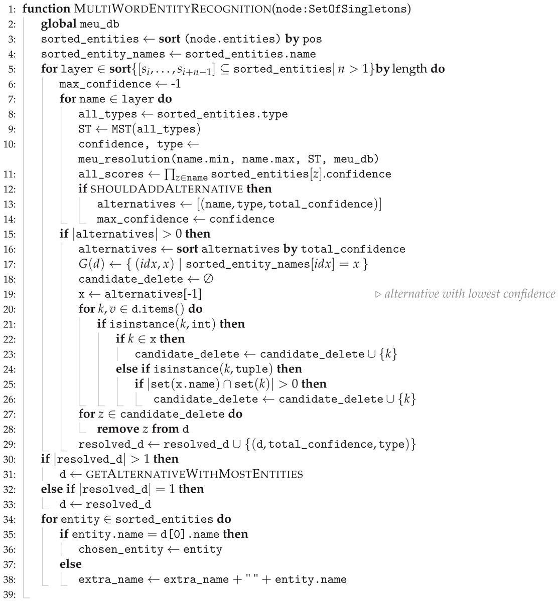
We now illustrate the proposed SetOfSingleton type according to the application order from the example given in Figure 5:
-
Multi-Word Entities: Algorithm 1 performs node grouping [66] over the the nodes connected by compound edge labels while efficiently visiting the graph using a Depth-First Search (DFS) search. After this, we identify whether a subset of these nodes acts as a specification (extra) to the primary entity of interest or whether it should be treated as a single entity. This is computed as follows: after generating all the possible ordered grouping of words, we associate each group to a type as derived by their corresponding meuDB match. Through the typing information, we then decide to keep the most specific type as the main entity, while leaving the most general one as a specification (extra). While doing so, we also consider the confidence of the fuzzy string matching through the meuDB. Appendix A.1 provides further algorithmic details on how LaSSI performs this computation.Example 1.After coalescing thecompoundrelationships from Figure 5, we would like to represent the grouping “Newcastle city centre” as a Singleton with a core entity “Newcastle” and anextra“city centre”. Figure 6 sketches the main phases of Algorithm 1 leading to this expected result. For our example, the possible ordered permutations of the entities withinGROUPINGare: “Newcastle city”, “city centre”, and “Newcastle city centre”. Given these alternatives, “Newcastle city centre” returns a confidence of 0.8 and “city centre” returns the greatest confidence of1.0, so our chosen alternative is [city,centre]. As “Newcastle” is the entity having the most specific type, this is selected as ourchosen_entity, and subsequently, “city centre” becomes theextraproperty to be added to “Newcastle”, resulting in our finalSingleton: Newcastle[extra:city centre].For Simplistic Graphs, “Newcastle upon Tyne” would be represented as oneSingletonwith noextraproperty.
- Multiple Logical Functions: Due to the impossibility of graphs to represent n-ary relationships, we group multiple adverbial phrases into one SetOfSingleton. These will be then semantically disambiguated by their function during the Logical Sentence Analysis (Section 3.2.3). Figure 5 provides a simple example, where each MULTIINDIRECT contains either one adverbial phrase or a conjunction. Appendix A.2 provides a more compelling example, where such SetOfSingleton actually contains more Singletons.
-
Coordination: For coordination induced by conj relationships, we can derive a coordination type to be AND, NEITHER, or OR. This is derived through an additional cc relationship on any given node through a Breadth-First Search (BFS) that will determine the type.Last, LaSSI also handles compound_prt relationships; unlike the above, these are coalesced into one Singleton as they represent a compound word: becomes , and are not therefore represented as a SetOfSingleton.
| Algorithm 1 Given a SetOfSingletons node, this pseudocode shows how it is merged, while also determining whether an `extra’ should be added to the resulting merged Singleton node. |
 |
3.2. Ad Hoc
This phase provides a gradual ascent of the data representation ladder through which raw full text data are represented as logical programs, thus achieving the most expressive representation of the text. As this provides an algorithm to extract a specification from each sentence, providing both a human- and machine-interpretable representation, we refer to this phase as an ad hoc explanation phase, where information is “mined” structurally and semantically from the text.
The transformation function, , takes our full text enriched with semantic information from the previous phase and rewrites it into a final suitable format whereby a semantic similarity metric can be used: either a vector-based cosine similarity, which is a traditional graph-based similarity metric where both node and edge similarity are given through vector-based similarity, potentially capturing the logical connectives represented within each node; or our proposed support-based metric requiring a logical representation for the sentences. These are then used to account for a different transformation function : when considering classical vector-based transformers, we consider those available through the HuggingFace library. For our proposed logical approach, the full text must be transformed as we need a representation that the system can understand to calculate an accurate similarity value produced from only relevant information.
To obtain this, we have distinct subsequent rewriting phases, where more contextual information is gradually added on top of the original raw information: after generating a semistructured representation of the full text by enriching the text with UDs as per Stanford NLP (Input in Figure 7, Supplement I.1), we apply a preliminary graph rewriting phase that aims to generate similar graphs for sentences, where one is the permutation of the other or simply differs from the active/passive form (Result in Figure 7, Section 3.2.1). At this stage, we also derive a cluster of nodes (referred to as the SetOfSingletons) that can be used later on to differentiate the main entity to the concept that the kernel entity is referring to (Appendix A.2.1). After this, we acknowledge the recursive nature of complex sentences by visiting the resulting graph in topological order, thus generating minimal sentences first (kernels) to then merge them into a complex and nested sentence structure (Section 3.2.2). After this phase, we extract each linguistic logical function occurring within each minimal sentence using a rule-based approach exploiting the semantic information associated with each entity as derived from the a priori phase (Section 3.2.3). This then leads to the final logical form of a sentence (Section 3.2.4), generating the following logical representation for Figure 7:
3.2.1. Graph Rewriting with the Generalised Semistructured Model (GSM)
This step employs the proposed GSM [67] to refine the initial graph and capture shallow semantic relationships, merely acknowledging the syntactic nature of the sentence without accounting for the inner node semantic information. Traditional graph rewriting methods, such as those for property graphs [68], are insufficient for our needs. They struggle with creating entirely new graph structures or require restructuring existing ones. To overcome these limitations, we leverage graph grammars [65] within the DatagramDB framework. The DatagramDB database rewrites the initial graph represented using a GSM data structure, incorporating logical connectives and representing verbs as edges between nodes as shown in Figure 7; among the other operations, this phase normalises active and passive verbs by consistently generating one single edge per verb. Here, the source identifies the entity performing the action described by the edge label. For transitive verbs, the targets might provide information regarding the entity receiving the action from the agent. This restructuring better reflects the syntactic structure and prepares the graph for the final logical rewriting step. If this does not occur, we either flatten out each SetOfSingleton node into one Singleton node (SGs) or we only retain the logical connectors and flatten out the rest (LGs). Thus, all forthcoming substeps are considered relevant to obtaining only the final logical representation of a sentence (Section 3.2.2, Section 3.2.3, and Section 3.2.4). Given that the scope of our work is on the main semantic pipeline and not on actual graph rewriting queries, which were already analysed in our previous work [65], we refer to the online query for more information on the rewriting covered by our current solution (https://github.com/LogDS/LaSSI/blob/32ff1df2df7d824619f9a84e7ae7d7f6e4842cb0/LaSSI/resources/gsm_query.txt, Accessed on 29 March 2025).
3.2.2. Recursive Relationship Generation
In this phase, we carry out some additional graph rewriting operations that generate binary relationships representing unary and binary predicates by considering semantic information for both edge labels and the topological orders of the sentences. While the former are clearly represented as binary relationships with anonetarget argument and usually refer to intransitive verbs, the latter are usually associated with transitive verbs. Either subjects or targets explicitly missing from the text and not expressed as pronouns are resolved as fresh variables, which will then be bound in the logical rewriting phase into an existential quantifier. Given that this phase also needs to consider semantic information, this rewriting cannot be completely covered by any graph grammar or general GQL and, therefore, cannot be entirely addressed in the former phase. This motivates us to hardcode this phase directly in a programming language rather than flexibly represent this through rewriting rules like any other phase within the pipeline.
Unlike in our previous contribution [16], we now cover the recursive nature of subordinate clauses [40] by employing a DFS topological sort [69], whereby the deepest nodes in our graph are accounted for first. This can be implemented because every graph is always acyclic; previously, no pre-processing occurred and the graph was read in directly from the rewritten GGG output. The topological sort induces layering on the graph, for which all the siblings of a given node belong to the same layer. Since any operations on the children can be carried out in any order, as they have no dependencies, there are no strict requirements on the order in which the children should appear. By sorting the nodes, we minimise the changes by starting from the nodes with fewer dependencies with the other constituents [65].
Example 2.
Figure 8 shows an example output from DatagramDB. The generated JSON file lists the IDs in the following order: 1, 6, 7, 8, 9, 10, 11, 12, 5, 2, 3. However, once our topological sort is performed, this becomes 3, 1, 2, 6, 7, 9, 5, 8, 10, 11, 12, where our `deepest’ nodes are at the start of the list, and each lower layer follows. Subsequent filtering culls nodes from the list that are no longer needed: The edge label between nodes 1 and 3 isinherit_edge, which means all properties of node 3 are added to node 1, and thus, node 3 is removed. Nodes 12 and 8 contain no information, so they can also be removed. Finally, node 2 (to) has already been inherited into the edge label “toanswer”, so it is also removed (because it does not have any parents or children). This results in the final sorted list: 1, 6, 7, 9, 5, 10, 11. Our list ofnodeswithin the pipeline is kept in this topological order throughout. Therefore, we can retrieve all roots from the graph to create our kernels.
Unlike the previous simplistic example, most real-world sentences often have a hierarchical structure, where components within the sentence depend on prior elements [65]. Topological sorts then take care of these more complex situations.
| Algorithm 2 After our a priori phase, we move to creating our final kernel. This is how our sentence is represented before transforming into our final logical representation. |
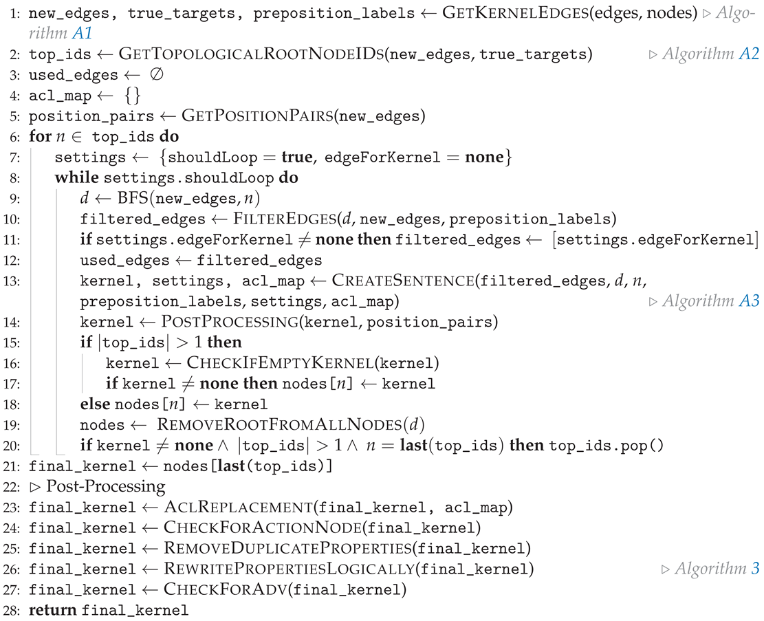 |
Algorithm 2 sketches the implementation of this phase, where more detailed information is given in Appendix B for conciseness, nesting the different relationships retrieved through a Singleton. After identifying which edges are the candidates (containing verbs) to become relationships (edges, Line 1), which are the main entry points for each of these to extract a relevant subgraph (top_ids, Line 2), we can now create all relationships representing each verb from the full text to then connect them into a single Singleton-based tree. After initialising the pre-conditions for the recursive analysis of the sentences (settings on Line 7) for each sentence entry point to be analysed (n, an ID), we collect all relevant nodes and edges associated with it: d, all descendant nodes of n retrieved from a BFS from our new_edges (see Algorithm A1). We then filter the edges by ensuring the following: the source and target are contained within the descendant nodes (d) or the target node is in our preposition labels, and the source and target have not already been used in a previous iteration or they have been used in a previous iteration but we have at least one preposition label within the text (Line 10). However, if our loop settings contain a relationship, we use it as our filtered_edges, as we need to create a new one.
CreateSentence only handles the rewriting of at most one kernel, whereas another may be contained within its properties; therefore, we handle this by returning a possible new kernel through settings.edgeForKernel and create a new sub-sentence to be rewritten with the same root ID, which is determined from our conditions set out in Appendix B.3. At this stage, we assign our used_edges to our collected filtered_edges for the next (possible) iteration.
After considering only the edges relevant to generating logical information for the sentence and after electing the relevant one among those to become a relationship across Singletons as our kernel (Line 13), we further refine the content of the selected edge and carry out a post-processing phase also considering semi-modal verbs [70] (Line 14). We also check if we have multiple verbs leading to multiple relationships generating new kernels; if so, we check if this current relationship has no appropriate source or target (Line 16). We refer to these relationships as empty. However, we check within the properties of this kernel to see if a kernel is present within these properties and whether this can be used as our new kernel instead. Following this, we remove all root properties from the nodes used in this iteration to avoid being considered in the next step and produce duplicate rewritings. Finally, if we are considering more than one kernel, and the last rewritten kernel is none, then we remove it to ensure that the last successfully rewritten kernel is used for our final kernel. The kernel is selected by taking the ID of the last occurring ID in top_ids, which is the first relationship in topological order for a given full text (Line 21). Finally, we check if the edge label is a verb; if not, it is replaced with none. Otherwise, we return the kernel.
The final stage of the kernel creation is additional post-processing to further standardise the final sentence representation: after resolving the pronouns with the entities they are referring to (Line 23), we generate relationships as verbs as either occurring as edge graphs or node properties (Line 24). After cleaning redundant properties, (Line 25), we rewrite such properties as Logical Functions of the sentence (Line 26, Section 3.2.3). Last, we associate propositions to the verbs when forming phrasal verbs (Line 27).
Supplement I.2 provides further implementation details.
3.2.3. Logical Sentence Analysis
Given the properties extracted from the previous phase1, we now want to rewrite such properties by associating each occurring entity with its logical function within the sentence and recognising any associated adverb or preposition while considering the type of verb and entity of interest. This rewriting mechanism exploits simple grammar rules found in any Italian linguistic book (see Section 2.3.1), and is therefore easily accessible. To avoid hardcoding these rules in the pipeline, we declaratively represent them as instances of LogicalRewriteRule concepts within our Parmenides ontology (Figure 9a). These rules can be easily defined in Horn clauses (Figure 9b), thus making them easy to implement. Thus, we can then easily extend LaSSI to support further logical functions by extending the rules within the ontology rather than changing the codebase.
Example 3.
Concerning Listing 9a, we are looking for a property that contains a preposition of either “in” or “into”, and is not an abstract concept entity. An example sentence that would match this rule is “characters in movies”. Before rewriting with Algorithm A5, we obtainbe(characters, ?)[nmod(characters, movies[2:in])]. Thenmodedge is matched to the rewriting rule, and is thus rewritten based on the properties of the matched logical function, presented in Listing 9c, whereby it should be attached to the kernel, resulting inbe(characters, ?1)[(SPACE:movies[(type:stay in place)])]
.
The entailed semantics for the application of these rules are like in Algorithm 3: For each relationship k generated in the previous phase, we select all the Singletons (Line 8) and SetOfSingletons (Line 18) within its properties. For each of the former, we consider them in declaration order (rule order), and once we find a rule matching some preconditions (premise), we apply the rewriting associated with it and skip the testing for the other rules. When such a condition is met, we establish an association between the logical function determined by the rule and the matched Singleton or SetOfSingletons within the relationship properties. If this is differently stated at the level of the rule, we then move such a property to the level of the properties of another Singleton within the relationship of interest (Figure 9c). We perform these steps recursively for any further nested relationship as part of the properties (Line 17).
| Algorithm 3 Properties contained within the kernel at this stage are not entirely covered logically. Therefore, this function determines, under a set of rules within the text, how they should be rewritten and appended to the properties of the kernel in order to be properly represented. |
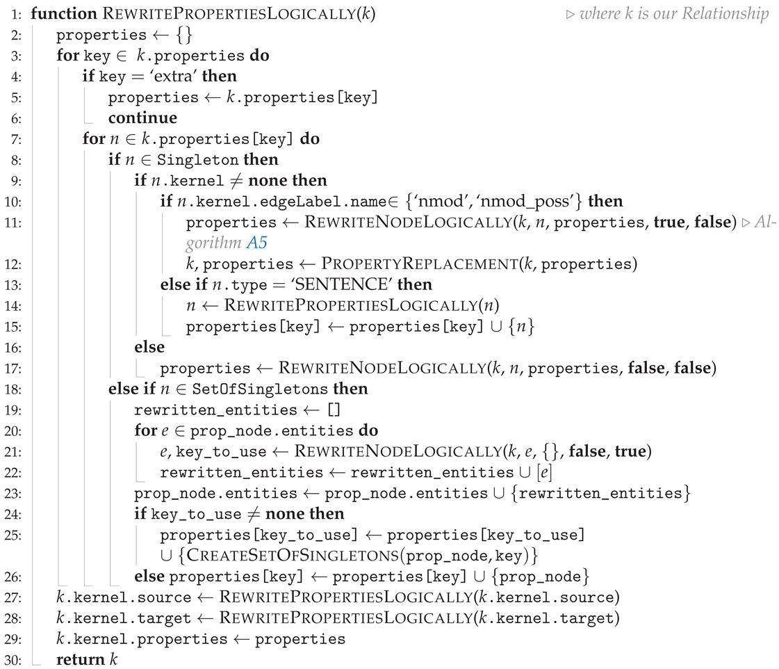 |
Example 4.
`Group of reindeer’ is initially rewritten as
be(group, ?)[(nmod(group, reindeer[(2:of)]))]
After determining the specification as per Line 11, we obtain some redundancies:
be(group, ?)[SPECIFICATION:group[(extra:reindeer)[2:of]]]
We have the source containinggroup, with properties that are also of the same entity, but with the additional information ofreindeer; therefore, on Line 12, we replace the source with the property and subsequently obtain:
be(group[(extra:reindeer)[2:of]], ?)
Rule premises may include prepositions from case [71] properties like `of’, `by’, and `in’, or predicates based on verbs from nmod [72] relationships, and whether they are causative or movement verbs. There are many different types, like `space’ and `time’, and the property further clarifies the type. For `space’, you might have `motion to place’, implying the property has a motion from one place to another, or `stay in place’, indicating that the sentence’s location is static. For time, we might have `defined’ for `on Saturdays’ or `continuous’ for `during’, implying the time for the given sentence has yet to occur (Table 1).
Example 5.
The sentence “Traffic is flowing in Newcastle city centre, on Saturdays” is initially rewritten asflow(Traffic, None)[(GPE:Newcastle[(extra:city centre), (4:in)]), (DATE:Saturdays[(9:on)])]. We have both the location of “Newcastle” and time of “Saturdays”. Given the rules from Figure 9a, the sentence would match theDATEproperty andGPE. After the application of the rules, the relationship is rewritten as
flow(Traffic, None)[(SPACE:Newcastle[(type:stay in place), (extra:city centre)]), (TIME:Saturdays[(type:defined)])]
Due to lemmatisation, the edge label becomesflowfrom “is flowing”.
For conciseness, additional details for how such a matching mechanism works are presented in Appendix C.
3.2.4. Final First-Order Logic (FOL) Representation
Finally, we derive a logical representation in FOL. Each entity is represented as one single function, where the arguments provide the name of the entity, its potential specification value, and any adjectives associated with it (cop), as well as any explicit quantification. These are pivotal for spatial information from which we can determine if all the parts of the area () or just some of these () are considered. This characterisation is not represented as FOL universal or existential quantifiers, as they are only used to refine the intended interpretation of the function representing the spatial entity. Transitive verbs are then always represented with binary propositions, while intransitive verbs are always represented as unary ones; for both, their names refer to the associated verb name. If any ellipsis from the text makes an implicit reference to either of the arguments, these are replaced with a fresh variable, which is then bound with an existential quantifier. For both functions and propositions, we provide a minor syntax extension that does not substantially affect its semantics, rather than use shorthand to avoid expressing additional function and proposition arguments referring to further logical functions and entities associated with them. We then introduce explicit properties p as key–value multimaps. Among these, we also consider a special constant (or 0-ary function) None, identifying that one argument is missing relevant information. We then derive the following syntax, which can adequately represent factoid sentences like those addressed in the present paper:
Throughout this paper, when an entity “foo” is associated with only a name and has no explicit all/some representation, this will be rendered as . When “foo” comes with a specification “bar” and has no explicit all/some representation, this is represented as .
Given the intermediate representation resulting from Section 3.2.2, we then rewrite any logical connective occurring within either the relationships’ properties or within the remaining SetOfSingletons as logical connectives within the FOL representation, and represent each Singleton as a single function. Each free variable in the formula is bound to a single existential quantifier. When possible, negations potentially associated with specifications of a specific function are then expanded and associated with the proposition containing such function as a term.
3.3. Ex Post
The ex post explanation phase details the similarity of two full text sentences through a similarity score over a representation derived from the previous phase. When considering traditional transformer approaches representing sentences as semantic vectors, we consider traditional cosine similarity metrics (Section 3.3.1). When considering graphs representable as collections of edges, we consider alignment-driven similarities, for which node and edge similarity is defined via the cosine similarity over their full text representation (Section 3.3.4).
3.3.1. Sentence Transformers
Vector-based similarity systems most commonly use cosine similarity for expressing similarities for vectors expressing semantic notions [73,74], as two almost-parallel normalized vectors will lead to a near-one value, while extremely dissimilar values lead to negative values [75]. This induces the possibility of seeing zero as a threshold boundary for separating similar from dissimilar data. This notion is also applied when vectors represent hierarchical information [76] with some notable exceptions [77]. Given A and B are vector representations (i.e., embeddings) from a transformer for sentences and , this is . Still, a proper similarity metric should return non-negative values [19]. Given the former considerations, we can consider only values above zero as relevant and return zero otherwise, thus obtaining:
Different transformers generate different vectors, automatically leading to different similarity scores for the same pair of sentences.
3.3.2. Neural IR
When considering neural IR approaches, we require an extra loading phase, where all the sentences within the datasets are treated as the corpora of documents to be considered. Then, the documents are indexed through their associated vectors. In this scenario, we also consider the same sentences as the queries of interest. As ColBERTv2 yields , which is a set of vectors for a given sentence , the authors defined the ranking score as , which is not necessarily normalised between 0 and 1. We now consider the following normalisation:
where m and M, respectively, denote the minimum () and the maximum () query-document alignment score.
3.3.3. Generative Large Language Models (LLM)
When considering classifiers such as DeBERTaV2+AMR-LDA based on a generative LLM, we express the classification for the sentence pair and as “”, which is then used in the classification task. Any other unexpected representation of sentences may lead to misleading classification results; for example, changing the prompts to “if then ” leads to completely wrong results. This returns a confidence score per predicted class k: . Thus, the class predicted is the one associated with the highest score; that is, . As the representation of interest only classifies logical entailment2 () or indifference (), and given that all former approaches work under the assumption that the same given score alone can be used to determine the similarity of two sentences, we map the predicted score for the logical entailment class between 0.5 and 1. In contrast, we map the indifference score between 0 and 0.5.
3.3.4. Simple Graphs (SGs) vs. Logical Graphs (LGs)
Given that our graphs of interest can be expressed as a collection of labelled edges, we reduce our argument to edge matching [15]. Given an edge distance function , an edge e, and a set of edges A obtained from the pipeline as a transformation of the sentence, the best match for e is an edge minimising the distance , i.e., . We can then express the best matches of edges in A over another set as a set of matched edge pairs . Then, we denote as the set of edges not participating in any match. The matching distance between two edge sets shall then consider both the sum of the distances of the matching edges as well as the number of the unmatched edges [19]. Given an edge-based representation A and B for two sentences and generated like in Section 3.2.1, we derive the following edge similarity metric as the basis of any subsequent graph-based matching metric:
Given a node representing a (SetOf)Singleton(s) , an edge label , and normalised similarity metric ignoring the negation information, we refine from Eq. 2 by conjoining the similarity among the edges’ sources and targets, while considering edge label information. We annihilate such similarity if the negations associated to the edges do not match by multiplying such similarity by 0; then, we negate the result for transforming this similarity into a distance:
where represents an edge, and , its associated label. This metric can be instantiated in different ways for simplistic graphs and LGs using a suitable definition for and .
Simple Graphs (SGs)
For graphs, all SetOfSingletons are flattened to Singletons, including the nodes containing information related to logical operators. In these cases, we use and as from Equation (1). At this stage, we still have a symmetric measure.
Logical Graphs (LGs)
We introduce notation from [19] to guarantee the soundness of the normalisation of distance metrics: we denote the normalisation of a distance value between 0 and 1, and its straightforward conversion to a similarity score.
Now, we extend the definition of from Eq. 3 as a similarity where is the associated distance function defined in Eq. 4, where we leverage the logical structure of SetOfSingletons. We approximate the confidence metric via an asymmetric node-based distance derived using fuzzy logic metrics with matching metrics for score maximisation. We return the maximum distance 1 for all the cases when one logical operator cannot necessarily entail the other.
3.3.5. Logical Representation
At this stage, we must derive a logic-driven similarity score to overcome the limitations of current symmetrical measures that cannot capture logical entailment. We can then re-formulate the classical notion of confidence from association rule mining [17], which implicitly follows the steps of entailment and provides an estimate for conditional probability. From each sentence and its logical representation A, we need to derive the set of circumstances or worlds in which we trust the sentence will hold. As confidence values are always normalised between 0 and 1, these give us the best metric to represent the degree of trustworthiness of information accurately. We can then rephrase the definition of confidence for logical formulae as follows:
Definition 6
(Confidence). Given two logically represented sentences A and B, let and represent the set of possible worlds where A and B hold, respectively. Then, the confidence metric, denoted as , is defined based on its bag semantics as:
Please observe that the only formula with an empty set of possible worlds is logically equivalent to the universal falsehood ⊥; thus, .
The forthcoming paragraphs contextualise the way to derive the computation of the formula using our Parmenides ontology and the Closed-World Assumption (CWA) to ensure the correctness of the inference.
Tabular Semantics per Sentence
Given the impossibility of potentially enumerating all the possible infinite conditions where a specific situation might hold, we focus our interest on the worlds encompassed by the two formulae considered within the application of the confidence function. After extracting all the unary or binary atoms occurring within each formula and logical representation A, we can only consider the set of possible worlds covered by the truth or falsehood of each of these atoms. Thus, the set of all possible worlds where A holds is the set of the worlds where each of the atoms within the formula holds while interpreting each formula using Boolean-valued classical semantics [78]. Such semantics are showcased in Example 7.
Example 7.
Consider the sentences : “Alice plays football” and : “Bob plays football”. We can represent these logically as binary propositions and , respectively. Given the sentences α: “Alice and Bob play football” and β: “Either Alice or Bob play football”, we can see that the former propositions can be considered atoms defining the current sentences. We then represent them as and , where both . Thus, we can easily derive the set of the possible worlds from the ones arising from all the possible combinations of the truth and falsehood of each proposition, as shown in Table 3: Thus, given the corresponding truth table from Table 3, we derive the following values for the bag semantics of A and B: and .
Appendix D.1 formalises the definition of the tabular semantics in terms of relational algebra, thus showcasing the possibility of enumerating all the worlds for which one formula holds while circumscribing them to the propositions that define the formula.
Determining General Implications Through Machine Teaching
As a next step, we want to derive whether each atom occurring in each formula A entails (implication), is equivalent to (bijective implication), is indifferent to (indifference, or is inconsistent (inconsistency) to another atom in the other formula of interest. As the atoms in the original sentence can be further decomposed into other atoms that are either equivalent or logically entailing the former, to control that the machine produces sensible and correct rules from the data given, we exploit machine teaching techniques [22,23] to ensure the machine derives correct propositions by exploiting a human-in-the-loop approach [24]. To achieve this, we opt for rule-based semantics [1,14], expanding each distinct atom and in the full text. We exploit this as a common approach when designing Upper Ontologies [21], where TBox reasoning rules are hardcoded to ensure the correctness of the inference approach.
Given the inability of description logic to represent matching and rewriting statements [79] and given the lack of support flexible properties associated with predicates of current knowledge expansion algorithms that require a fixed schema [1,14], we perform this inference by exploiting an explicit pattern matching and rewriting mechanism. To achieve this, we exploit the Python library FunctionalMatch (https://github.com/LogDS/FunctionalMatch/releases/tag/v1.0, Accessed on 30 March 2025) as a derivation mechanism generating propositions out of the expansion rules of interest representing common-sense information and relationships between the entities. We then apply expansion rules and , where the first derives a set of logically entailing propositions , while the latter derives a set of equivalent propositions .
At this stage, we define the semantic equivalence between the expanded propositions using the Parmenides KB, thus deriving a merely semantic correspondence between such propositions. For conciseness, this is detailed in Appendix D.2. This provides a discrete categorisation of the general relationships that might occur between two propositions while remarking whether one entails the other (), if they are equivalent (), if they are inconsistent (), or if they are indifferent (). Unlike in our previous paper, we then categorise the previous cases in order of priority as follows:
- Equivalence:
- if is structurally equivalent to .
- Inconsistency:
- if either or is the explicit negation of the other, or whether their negation appears within the expansion of the other ( and , respectively).
- Implication:
- if occurs in one of the expansions .
If none of the above conditions holds, we compare the and the expanded propositions. Given , the function prioritising the comparison outcomes over a set of compared values (Equation (A4) in the Appendix), we obtain the comparison outcome as: . After this, we associate each pair of propositions with a relational table from Figure 10, from which we select only the possible worlds of interest where it is plausible to find the worlds occurring, where indifference is derived if none of the above conditions holds.
By naturally joining all the derived tables together into , including the tabular semantics associated with each formula A and B, we trivially reason paraconsistently by only considering the worlds that do not contain contradicting assumptions [80]. We express confidence from Equation (5) as follows:
While the metric summarises the logic-based sentence relatedness, provides the full possible world combination table for the number derived. By following the interpretation of the support score, we then derive a score of 1 when the premise entails the consequence, 0 when the implication derives a contradiction, and any value in between otherwise, noting the estimated ratio of possible worlds as stated above. Thus, the aforementioned score induces a three-way classification for the sentences of choice.
Example 8.
From Table 3 and Example 7, we can use these values to determine the confidence value when and . In our scenario, the resulting equi-join matches the one from Table 3, as all the propositions are indifferent.
To first find , we find , meaning the number of times s and t are true, which is 1 when both a and b are true. Then, we find , the number of times s is true, which is also 1 when both a and b are true. Substituting into the confidence metric, we obtain , meaning that when a is true, it iscertainthat b is also true; like when Alice and Bob are playing football, it must therefore hold that either are playing.
Alternatively, to find ; we find , which is 1, the same when both a and b are true. Then, we find , the number of times t is true, which is 3 when either a or b are true. Substituting into the confidence metric, we obtain , meaning that when b is true, there is only a chance that a is true; aW when either Alice or Bob play football, one cannot be certain whetherbothare playing.
We refer to Section 5.3.4 for some high-level graphical representation of this phase.
4. Results
The Results section is structured as follows: First, we demonstrate the impossibility of deriving the notion of logical entailment via any symmetric similarity function (Section 4.1). We base our argument on the following observation: given that current symmetric metrics are better suited to capture sentence similarity through clustering due to their predisposition of representing equivalence rather than entailment, we show that assuming symmetrical metrics also leads to incorrect clustering outcomes, based on which dissimilar or non-equivalent sentences are grouped. Second, we provide empirical benchmarks showing the impossibility of achieving this through classical transformer-based approaches as outlined in the Introduction (Section 4.2). All of these components provide a pipeline ablation study concerning the different rewriting stages occurring within the ad hoc phase of the pipeline, while more thorough considerations addressing disabling the a priori phase are presented in the Discussion section (Section 5.2). Lastly, we address the scalability of our proposed approach by considering sub-sents of full text sentences appearing as nodes for the ConceptNet common-sense knowledge graph (Section 4.3).
The experiments were run on a Linux Desktop machine with the following specifications: CPU: 12th Gen Intel i9-12900 (24) @ 5GHz; memory: 32 GB DDR5. The raw data for the results, including confusion matrices and generated final logical representations, can be found on OSF.io (https://osf.io/g5k9q/, Accessed 28 March 2025).
4.1. Theoretical Results
As the notion of verified AI incentivises inheriting logic-driven notions for ensuring the correctness of the algorithms [25], we leverage the logical notion of soundness [81] to map the common-sense interpretation of a full text into a machine-readable representation (as a logical rule or a vector embedding); a rewriting process is sound if the rewritten representation logically follows from the original sentence, which then follows the notion of correctness. For the sake of the current paper, we limit our interest to capturing logical entailment as generally intended from two sentences. Hence, we are interested in the following definition of soundness.
Definition 9.
Weak Soundness, in the context of sentence rewriting, refers to the preservation of the original semantic meaning of the logical implication of two sentences α and β. Formally:
where S is the common-sense interpretation of the sentence, ⊑ is the notion of logical entailment between textual concepts, and is a predicate deriving the notion of entailment from the τ transformation of a sentence through the choice of a preferred similarity metric .
In the context of this paper, we are then interested in capturing sentence dissimilarities in a non-symmetrical way, thus capturing the notion of logical entailment:
The following results imply that any symmetric similarity metrics (including cosine similarity and edge-based graph alignment) cannot be used to express logical entailment (Section 4.1.1), while the notion of confidence adequately captures the notion of logical implication by design (Section 4.1.2). All proofs for the forthcoming lemmas are presented in Appendix E.
4.1.1. Cosine Similarity
The above entails that we can always derive a threshold value above which we can deem as one sentence implying the other, thus enabling the following definition.
Definition 10.
Given α and β are full texts and τ is the vector embedding of the full text, we derive entailment from any similarity metric as follows:
where θ is a constant threshold. This definition allows us to express implications as exceeding a similarity threshold.
As cosine similarity captures the notion of similarity, and henceforth an approximation of a notion of equivalence, we can clearly see that this metric is symmetric.
Lemma 11.
Cosine similarity is symmetric
Symmetry breaks the capturing of directionality for logical implication. Symmetric similarity metrics can lead to situations where soundness is violated. For instance, if holds based on a symmetric metric, then would also hold, even if it is not logically valid. We derive implication from similarity when the similarity metric for is different to , given that , and this shows that one thing might imply the other but not vice versa. To enable the identification of implication across different similarity functions, we entail the notion of implication via the similarity value as follows.
Lemma 12.
All symmetric metrics trivialise logical implication:
Since symmetric metrics such as cosine similarity cannot capture the directionality of implication, they cannot fully represent logical entailment. This limitation highlights the need for alternative approaches to model implication accurately, thus violating our intended notion of correctness.
4.1.2. Confidence Metrics
In contrast to the former, we show that the confidence metric presented in Section 3.3 produces a value that aims to express logical entailment under the assumption that the transformation from the full text to a logical representation is correct.
Lemma 13.
When two sentences are equivalent, they always have the same confidence.
As a corollary of the above, this shows that our confidence metric is non-symmetric.
Corollary 14.
Confidence provides an adequate characterisation of logical implication.
This observation leads to the definition of the following notion of given , the processing pipeline.
Definition 15.
Given that α and β are the full text and τ is the logical representation of the full text derived in the ad hoc phase (Section 3.2), we derive entailment from any similarity metric as follows:
4.2. Clustering and Classification
While the previous section provided the basis for demonstrating the theoretical impossibility of achieving a perfect notion of implication, the following experiments aimed to test this argument from a different perspective. First, through clustering, we want to test which of these pre-trained language models is well suited for expressing the notion of logical equivalence. Given that the training-based approach cannot ensure a perfect notion of equivalence, returning a perfect score of 1 for extremely similar sentences, we can relax the argument by requiring that there exists any suitable clustering algorithm allowing us to group certain sentences based on distance values, providing the closest match to the group of expected equivalent sentences selected. According to Definition 10, we can then derive a minimum threshold value , with the minimum similarity score between the elements belonging to the same cluster derived from the chosen methodology.
Second, we want to show the ability of all such models to not only identify which sentences are equivalent but also ascertain their ability to differentiate between logical entailment, indifference, and inconsistent representation. To do so, we need to first annotate each sentence within our proposed dataset to indicate such a difference. Given that none of the proposed approaches were explicitly trained to recognise conflicting arguments, we then derive an upper threshold value separating the conflicting sentences from the rest by taking the maximal similarity score between the pair of sentences expected to be contradictory from the manual annotation. If , we consider only one threshold value separating entailing and contradictory data (). Thus, we consider all similarity values above prediction values for a logical entailment and all values lower than as predictive of a conflict between the two sentences. Otherwise, we determine an indifference relationship. Please observe that different clustering algorithms might lead to different scores: given this, we will also expect to see variations within the classification scores discussed in Supplement II.3 for this specific metric. Thus, our classification results will explicitly report the name of the paired clustering algorithm leading to the specific classification outcome.
As pre-trained language models are assumed to generalise their semantic understanding of the text through extensive training on a large corpus of data, these models should also be able to capture semantic and structural nuances provided in completely new datasets. To remove any semantic ambiguity derivable from analysing complex sentences with multiple entities, we considered smaller ones for controlled experiments under the different scenarios discussed in the Introduction (Figure 11a, Figure 13a, and Figure 15a) so provide empirical validation to preliminary theoretical results [52]. The set of sentences, alongside their expected clusters and classification outcomes, are freely available for reproducibility purposes (https://osf.io/g5k9q/, Accessed on 25 April).
We used the following transformers available on HuggingFace [82] from the current state-of-the-art research papers discussed in Section 2.4:
For all the approaches, we consider all similarity metrics as already normalised between 0 and 1, as discussed in Section 3.3. We can derive a distance function from this by subtracting the value from one; hence, . Since not all of these approaches lead to symmetric distance functions and given that the clustering algorithms work under symmetric distance functions, we obtain a symmetric definition by averaging the distance values as follows:
We test our hypothesis over two clustering algorithms supporting distance metrics as input rather than a collection of points in the d-dimensional Euclidean space, Hierarchical Agglomerative Clustering (HAC), and k-Medoids. The graphs visualised in Figure 12, Figure 14, and Figure 16 are dendrograms, which allow us to explore relationships between clusters at different levels of granularity as returned by HAC. For HAC, we considered the complete link criterion for which the distance between two clusters is defined as the distance between two points, each for one single cluster, maximising the overall distance [83]. We consider the k-Medoids algorithm with an initialisation procedure that is a variant of that of k-means++[84]. It considers the initial k-Medoids clusters to avoid poor initialisations resulting in the selection of weak initial random points by sampling these initial points over “an empirical probability distribution of the points’ contribution to the overall inertia” (https://scikit-learn.org/stable/modules/generated/sklearn.cluster.KMeans.html, Accessed on 29 March 2025). No further hyperparameter tuning is required under these assumptions, as these annihilate the need for carrying out multiple tests with multiple different random seeds. Supplement II.1 provides additional details for such clustering algorithms.
To ensure the correctness of the alignment score used to match the nodes in the graph semantically, we exploited this as a clustering measure and compared the score to others available in the current literature. In this case, rather than considering the alignment between a set of edges within the graph, we considered the alignment between sets of clusters. Thus, the correctness of the returned clustering match was computed using a well-defined set-based alignment metric from [19], which is a refinement of Equation (2) using , where is the indicator function returning 1 if and only if (iff) condition P holds and 0 otherwise [85]. We pair this metric with the classical Silhouette [86], Purity [53], and Adjusted Random Index (ARI) [87], as discussed in Supplement II.2.
4.2.1. Capturing Logical Connectives and Reasoning
We check if the logical connectives are treated as stop words and then ignored by transformers. This is demonstrated through sentences in Figure 11a, whereby one sentence might imply another, but not vice versa. However, with our clustering approaches, we only want to cluster sentences that are similar in both directions; therefore, our clusters have only one element, as shown in Figure 11b.
Figure 11.
Sentences and expected clusters for RQ №2(a), where no sentences are clustered together, as no sentence is perfectly similar to another in both directions.
Figure 11.
Sentences and expected clusters for RQ №2(a), where no sentences are clustered together, as no sentence is perfectly similar to another in both directions.
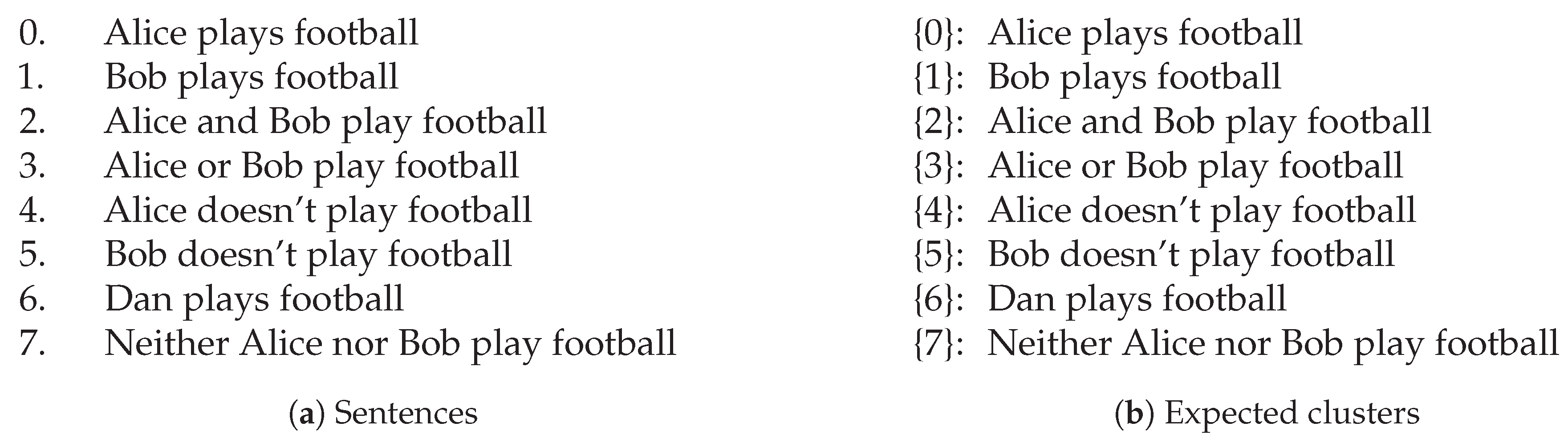
In Figure 12, we can see that for our SGs in Figure 12a, this approach fails to recognise directionality and does not produce appropriate clusters, even failing to recognise the similarity a sentence has with itself. The LGs shown in Figure 12b improve, recognising similarity for 2 ⇒ 0, for example; however, they indicate a similarity of 0 for 0 ⇒ 2. Finally, our logical representation in Figure 12c successfully identifies directionality and appropriately groups sentences together. For example, 2 ⇒ 0 is entirely similar; however, 0 ⇒ 2 is only slightly similar, which entails that “Alice and Bob play football” implies that “Alice plays football”, but it does not necessarily hold that both Alice and Bob play football if we only know that Alice plays football.
The sentence transformer approaches displayed in Figure 12d–g and all produce similar clustering results, with high similarities between sentences in the dataset that are incorrect; for example, the clusters of Alice does and does not play football are closely related according to the transformers. As mentioned above, this is most likely due to the transformers’ use of tokenisation, which removes stop words and, therefore, does not capture a proper understanding of the sentences. In contrast, our approach does this tby showing that they are dissimilar. DeBERTaV2+AMR-LDA (Figure 12h) has a dramatically different dendrogram from the others, showing very little notion of directionality and classifying the majority of sentences as completely dissimilar. This was unexpected for this approach, as it was explicitly trained to recognise logical entailment from simple factoid sentences. Moreover, ColBERTv2+RAGatouille (Figure 12i) shows a similar dendrogram to those of the sentence transformer approaches, with a wider range of confidence determining similarity, with 0 at its lower bound compared to ≈0.4 for the transformer approaches.
Figure 12.
Dendrogram clustering for RQ №2(a) sentences, where no clusters are highlighted, as there are none to present.
Figure 12.
Dendrogram clustering for RQ №2(a) sentences, where no clusters are highlighted, as there are none to present.
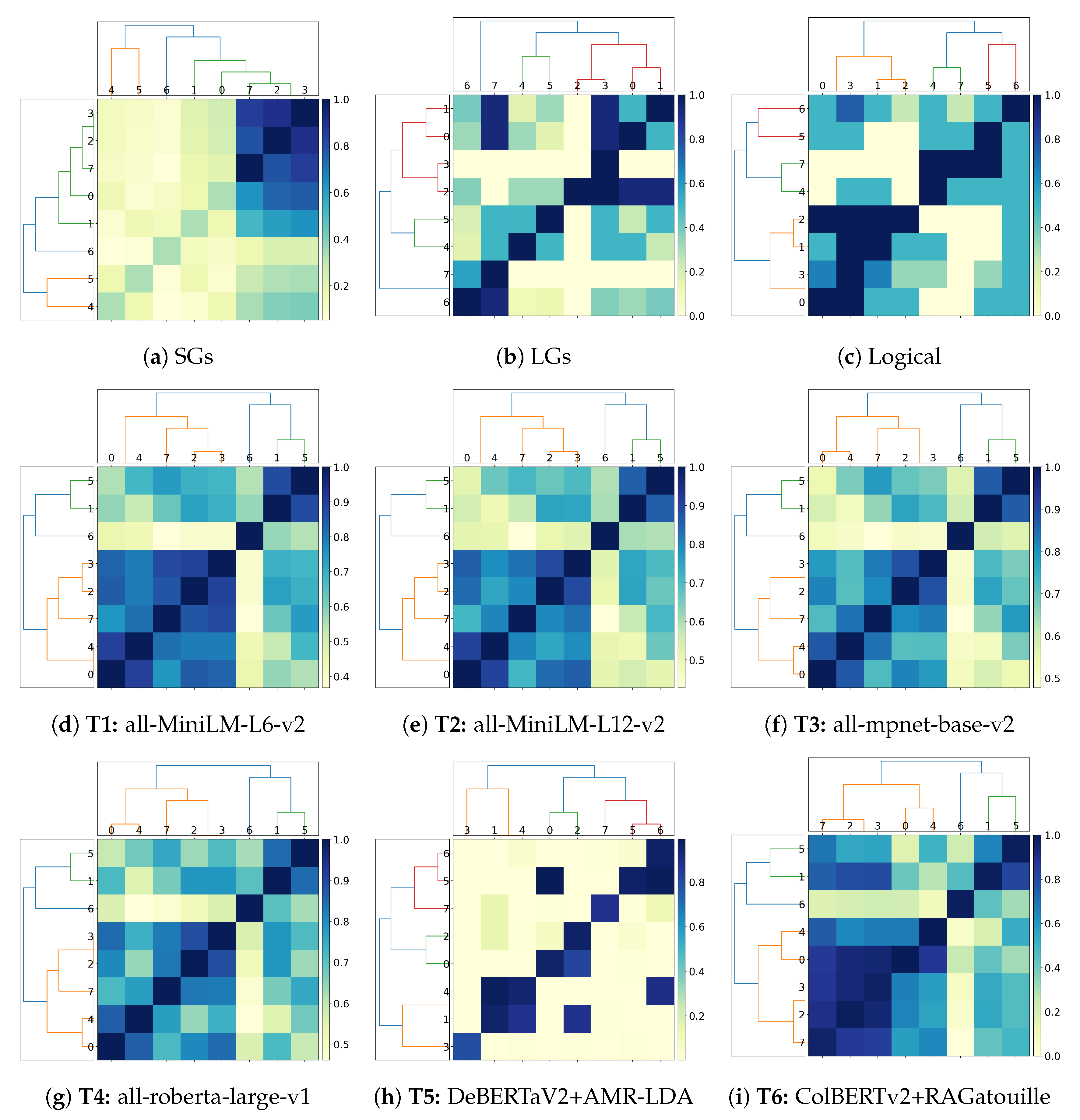
As for this dataset, we did not expect any clusters to form; the clustering experiments mainly aimed to determine whether any sensible clusters might be incorrectly derived. When analysing Table 4, almost all approaches perfectly align with the expected clusters when using HAC. However, this is determined by the nature of the algorithm as it starts with this exact configuration, where each element is its own cluster. It inherently matches the ground truth at the beginning; therefore, the algorithm achieves perfect alignment before any merging occurs. The silhouette score can only be calculated if the number of labels (sentences) is (https://scikit-learn.org/stable/modules/generated/sklearn.metrics.silhouette_score.html, Accessed 25 April 2025). In our case, the length of the clusters (8) is equal to the number of distinct labels (8); therefore, we cannot return the silhouette score. While using k-Medoids clustering, SG and DeBERTaV2+AMR-LDA (T5) yielded incorrect clusters, resulting in the grouping of sentences 2 and 3 and 1 and 4, respectively. This leads to the incorrect derivation of silhouette scores. For purity and ARI, we see perfect scores again when using HAC; only when using k-Medoids do we see a lower value for SGs and T5 (DeBERTaV2+AMR-LDA). As our SGs do not encompass logical connectives entirely, the clustering scores are expected to be lower.
In Table 5, we use both macro and weighted average scores, as all our datasets are heavily unbalanced. Furthermore, as different clustering algorithms might derive different upper threshold values , we kept the distinction between the different classification outcomes leading to a difference in classification. Our logical approach excels, achieving perfect scores across all classification scores. The preliminary stage of our pipeline, SG, achieves the worse scores across the board, thus clearly indicating that just targeting node similarity through node and edge embedding is insufficient for fully capturing sentence structure, even after GGG rewriting. LGs slightly improve over SGs due to the presence of a logical operation; this approach is shown to improve over classical sentence transformer approaches, with a few exceptions. In fact, ColBERTv2+RAGatouille provides better performances than other sentence transformers, and DeBERTaV2+AMR-LDA shows poor performance, thus indicating the unsuitability of this approach to provide reasoning over other logical operators not captured in the training phase. Moreover, our proposed logical representation improves over LGs through the tabular reasoning phase, due to the classical Boolean interpretation of the formulae: this indicates that graph similarity alone cannot be used to fully capture the essence of logical reasoning. In competing approaches, the weighted average is consistently lower compared to the macro average, thus suggesting that the misclassification task is not necessarily ascribable due to the imbalance nature of the dataset, while also suggesting that the majority class (indifference) was mainly misrepresented.
4.2.2. Capturing Simple Semantics and Sentence Structure
The sentences in Figure 13a are all variations of the same subjects (a cat and mouse), with different actions and active/passive relationships. The dataset is set up to produce sentences with similar words but in a different order, allowing for determination of whether the sentence embedding understands context from structure rather than edit distance. Figure 13b shows the expected clusters for the RQ №2(b) dataset. Here, 0 and 1 are clustered together as the subject’s action on the direct object is the same in both: “the cat eats the mouse” is equivalent to “the mouse is eaten by the cat”. Similarly, sentences 2 and 3 are the same, but with the action reversed (the mouse eats the cat in both).
Figure 13.
Sentences and expected clusters for RQ №2(b).
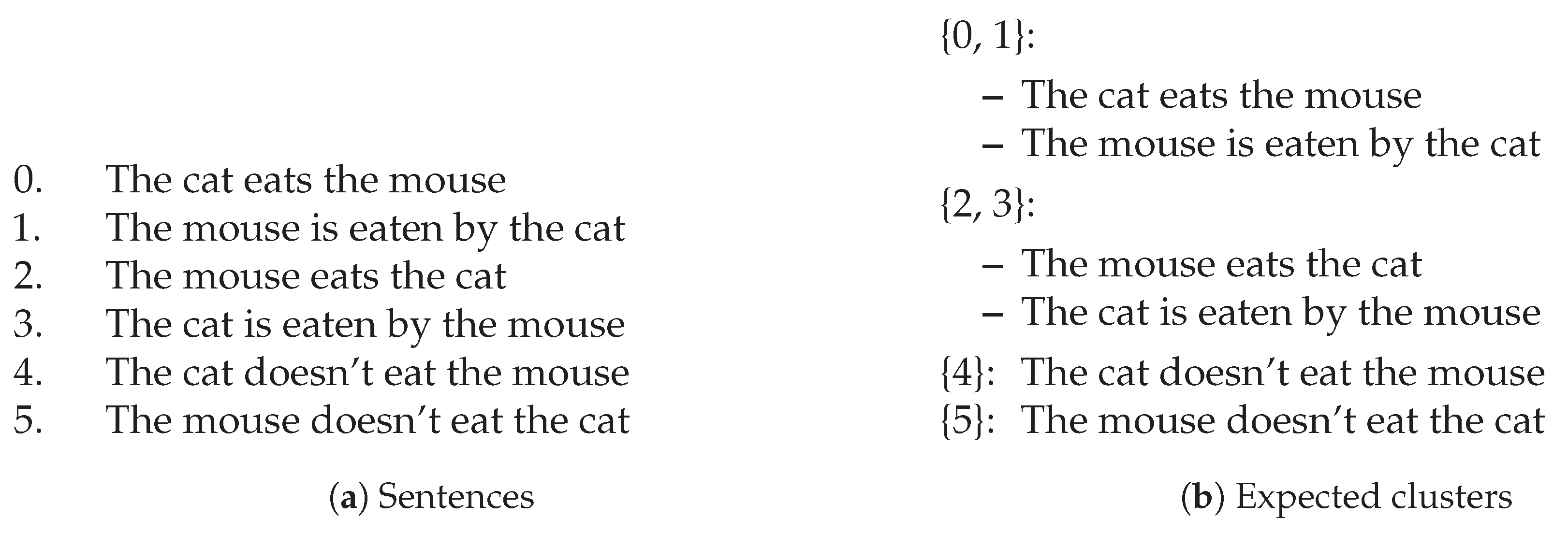
We can see a gradual increase in the number of matched clusters in Figure 14a–c, as the contextual information within the final representation increases with each different sentence representation. Each representation shows a further refinement within the pipeline. The clustering shows values that are near to each other, due to their structural semantics, but does not determine that they are the same. The first two approaches (SGs and LGs) roughly capture the expected clusters that we are looking for, but do not encapsulate the entire picture regarding the similarity of the sentences in the whole dataset. Meanwhile, our final logical representation produces the expected perfect matches with {0, 1}, and {2, 3}. This suggests that our proposed logical representation can identify the same relationship between the “cat” and “mouse”, despite different syntactic structures via active and passive voice. On the other hand, all pre-trained language models except for DeBERTaV2+AMR-LDA (T5) exhibited the following behaviour: clusters {0,2} and {1,3} always formed, thus suggesting that the attention mechanism favours the clustering of sentences around the verb, despite grouping together unrelated sentences. DeBERTaV2+AMR-LDA also made a similar choice by grouping together unrelated sentences: {0,5} and {2,4}.
Figure 14.
Dendrogram clustering for RQ №2(b) sentences, where red and orange boxes represent the clusters for {0,1} and {2,3} respectively. The classes are distributed as such: Implication: 10, Inconsistency: 8, Indifference: 18.
Figure 14.
Dendrogram clustering for RQ №2(b) sentences, where red and orange boxes represent the clusters for {0,1} and {2,3} respectively. The classes are distributed as such: Implication: 10, Inconsistency: 8, Indifference: 18.
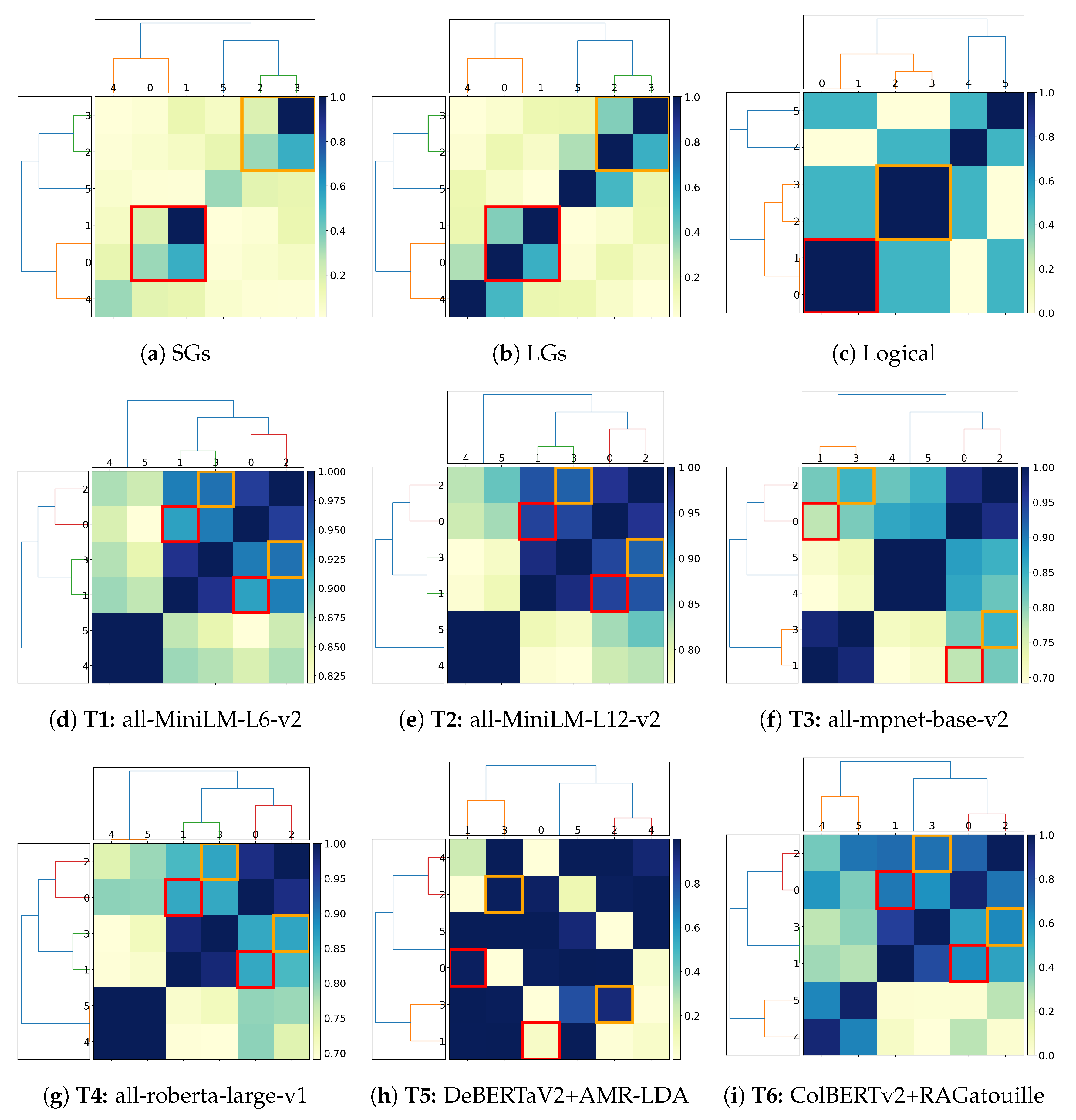
Analysing Table 6, we can see that all stages of the LaSSI pipeline achieved perfect alignment with HAC and k-Medoids, effectively capturing the logical equivalence between sentences 0 and 1, and 2 and 3. This was mainly ascribable to the GGG rewriting phase, which captures the notion of active vs. passive sentence, while rewriting the sentences in a uniform graph representation. Low silhouette scores for SGs and LGs indicate high intra-cluster heterogeneity with respect to similarity values. Furthermore, high levels of alignment, purity, and ARI demonstrate their ability to match the expected clusters. In agreement with the visual analysis of the dendrograms above, all pre-trained language models showed lower alignment with HAC and k-Medoids, thus including DeBERTaV2+AMR-LDA (T5). While they captured some semantic similarity, they struggled to fully grasp the logical equivalence between the sentences in the same way that LaSSI does, even with some simplistic rewriting using our pipeline. None of these transformers produced zones with 0 similarity, as they determined all the sentences to be related to each other, also misinterpreting that “The cat eats the mouse” and “The mouse eats the cat” as similar. The pipelines for these given transformers ignore stop words, which may also impact the resulting scores. We also recognise that the similarity is heavily dominated by the entities occurring, while the sentence structure is almost not reflected: transformers only consider one sentence to be a collection of entities without taking its structure into account, whereby changing the order will yield similar results and, therefore, sentence structure cannot be derived. Interpreting similarity with compatibility, graph-based measures entirely exclude the possibility of this happening, while logic-based approaches are agnostic.
Table 7 provides a more in-depth analysis of the situation where, instead of being satisfied with the possibility that the techniques mentioned above can capture the notion of equivalence between sentences, we also require that they can make finer-grained semantic distinctions. The inability of DeBERTaV2+AMR-LDA to fully capture sentence semantics might be reflected in the choice of the AMR representation as, in this dataset, the main differences across the data are based on the presence of negation and of sentences in both active and passive form. This supports the evidence that transformer-based approaches providing one single vector generally provide better results through masking and tokenisation. Differently from the previous set of experiments, subdividing the text encoding into multiple different sentences proved to be ineffective for the ColBERTv2+RAGatouille approach, as subdividing short sentences into different tokens for the derivation of a vector results in complete loss of the semantic information captured by the sentence structure. In this scenario, the proposed logical approach is mainly supported by tabular semantics, where most of the sentences are simply represented as two variants of atoms, potentially being negated. This indicates the impossibility of fully capturing logical inference through graph structure alone. In this scenario, precision scores appear almost the same, independent of the clustering and averaging technique. The Accuracy and F1 scores show that the similarity score is very near to a random choice.
4.2.3. Capturing Simple Spatiotemporal Reasoning
We considered multiple scenarios involving traffic in Newcastle, presented in Figure 15a, which have been extended from our previous paper to include more permutations of the sentences. This was done to obtain multiple versions of the same sentence that should be treated equally by ensuring that the rewriting of each permutation is the same, therefore resulting in 100% similarity. We consider this dataset as a benchmark over a part/existential semantics , thus assuming that all the potential quantifiers being omitted refer to an existential (e.g., somewhere in Newcastle, in some city centers, on some Saturdays). In addition, we consider negation as a flattening out process.
Figure 15.
Sentences and expected clusters for RQ №2(c).
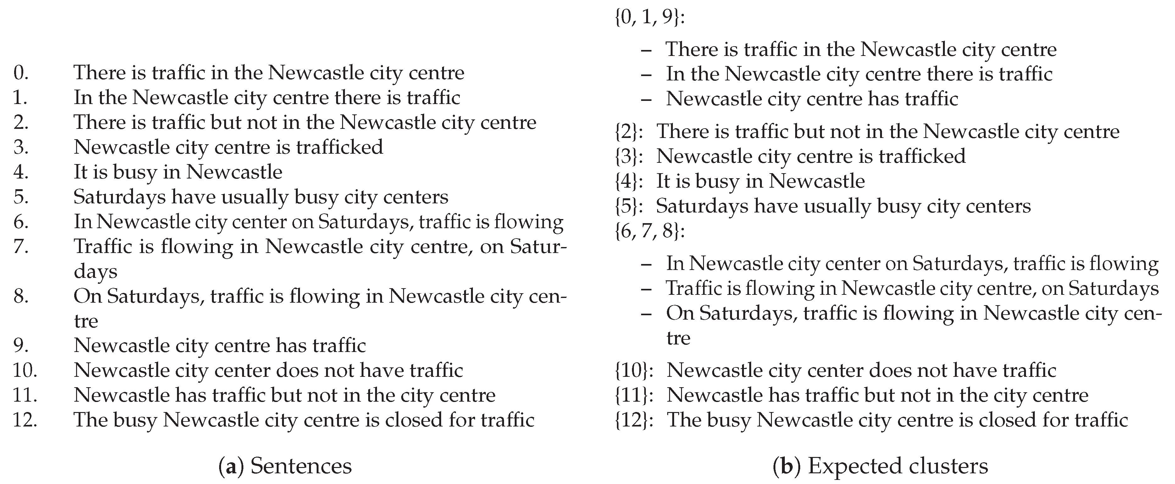
Figure 16.
Dendrogram clustering for RQ №2(c) sentences, where red and orange boxes represent the clusters for {0,1,9} and {6,7,8} respectively.
Figure 16.
Dendrogram clustering for RQ №2(c) sentences, where red and orange boxes represent the clusters for {0,1,9} and {6,7,8} respectively.
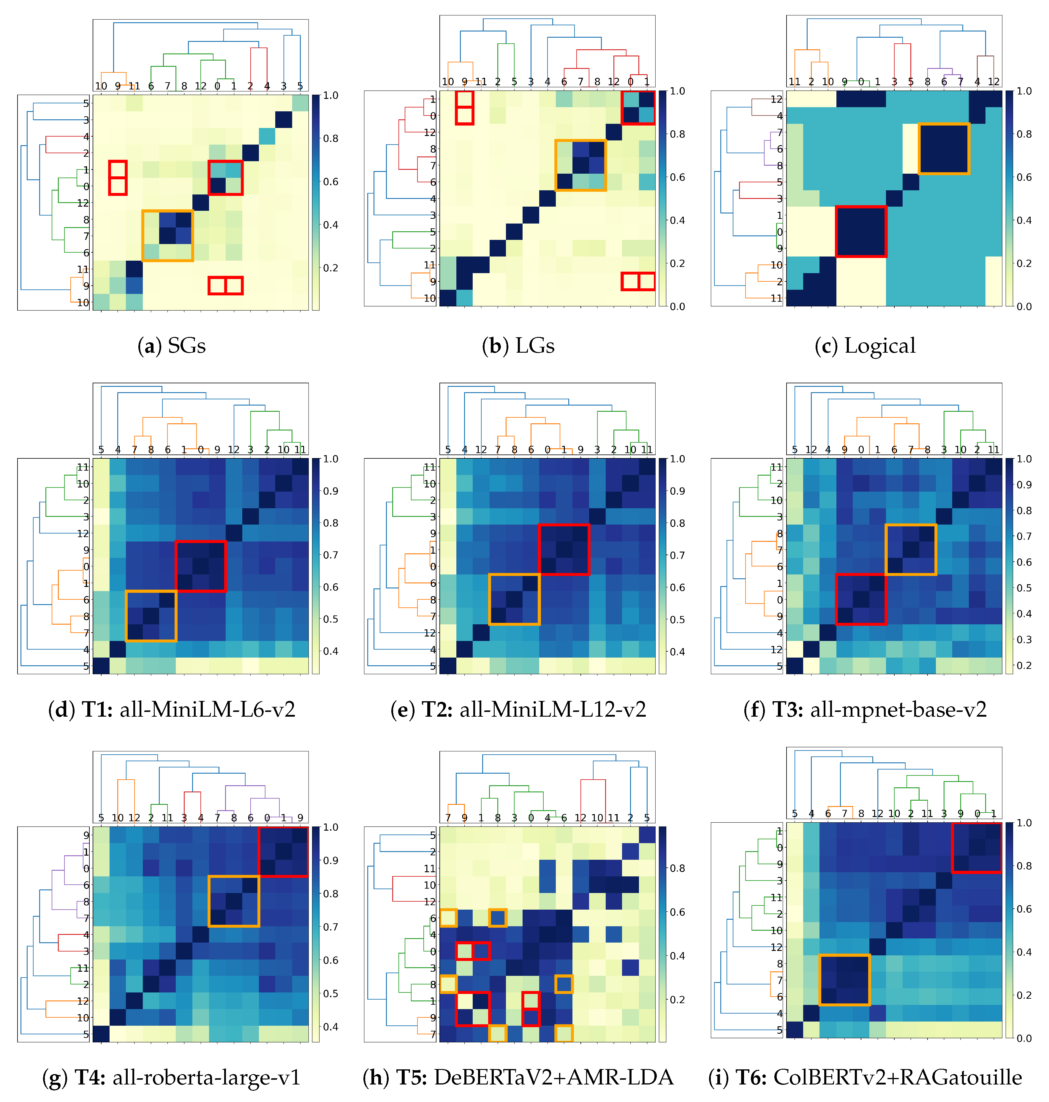
For the SGs in Figure 16a, we can see that some similarity was detected between sentences 7 (“Traffic is flowing in Newcastle city centre, on Saturdays”) and 8 (“On Saturdays, traffic is flowing in Newcastle city centre”), which is correct; however it should be treated as having 100% similarity, which it does not here. Furthermore, the majority of the dendrogram shows little similarity across the dataset. We see an increase in overall clustering similarity for both HAC and k-Medoids in the LGs approach, as shown in Figure 16b, now also capturing similarity between a few more sentences, but overall still not performing as expected. Finally, our logical approach presents an ideal result, with 100% clustering alignment and a dendrogram that presents clusters that match our expected outcome. {0,1,9} and {6,7,8} are clustered together, as we would expect, and we also see some further implications being presented.
The sentence transformer approaches produced a very high similarity for nearly all sentences in the dataset. There were discrepancies in the returned clusters, compared to what we would expect, for several reasons. The word embeddings might be capturing different semantic relationships. For example, “busy” in sentence 4 (“It is busy in Newcastle”) might be considered similar to the “busy city centers” in sentence 5 (“Saturdays have usually busy city centers”), leading to their clustering, even though the context of Newcastle being busy is more general than the usual Saturday busyness. We can see that sentences related to Saturdays (5, 6, 7, 8) form a relatively cohesive cluster in the dendrogram, which aligns with the desired grouping for 6, 7, and 8. However, sentence 5’s early inclusion with the general “busy” statement (4) deviates from the intended separation. Furthermore, the embeddings might be heavily influenced by specific keywords; for example, the presence of “Newcastle city centre” in multiple sentences might lead to their clustering, even if the context regarding traffic flow or presence differs. As discussed previously, these transformers could not differentiate between the presence and absence of traffic as intended in the desired clusters. For example, sentence 10 (“Newcastle city center does not have traffic”), was clustered with sentence 2 (“There is traffic but not in the Newcastle city centre”), which is incorrect.
Analysing the results in Table 8, we can see that our LGs and logical approaches outperformed the transformers, with our final logical approach achieving 100% alignment against the expected clusters. Differently from the previous experimental set-up (Table 6), the sentence transformer approaches exhibited generally good behaviour in terms of their purity and ARI score, while DeBERTaV2+AMR-LDA (T5) provided a consistently worse behaviour than the former. This is likely ascribable to the simplistic logic being used to train the system, making it unable to fully capture the semantic complexity of our proposed logic for describing the semantic behaviour through a Knowledge Base back-up (Appendix D.2.1), as well as not adequately rewriting the sentences to capture the equivalent sentences with different phrasing.
The clustering results now seem in line with the classification scores from Table 9: DeBERTaV2+AMR-LDA consistently provided low scores, being slightly improved by our preliminary simplistic SG representation. Despite the good ability of LGs to cluster the sentences, they less favourably capture correct sentence classifications, as (consistently with the previous results) they are outperformed by competing transformer-based approaches which, still, provided less than random scores in terms of accuracy. Even in this scenario, the competing approaches exhibited a lower weighted average compared to the macro one, thus indicating that the results were not biased by the unbalanced dataset.
4.3. Sentence Scalability Rewriting
We recorded the individual running times of each phase in the LaSSI pipeline for each sentence within the 200 sentences taken from ConceptNet [2]. We also recorded the sentence length, as characterised by the number of nodes in each graph representation of the sentence and its character length. Figure 17 plots the average number of vertices as sentence length increases, which almost presents a linear correlation. As the ad hoc phase of our pipeline operates on the graph representation of the sentence, rather than on its character length, while the GSM generation through StanfordNLP dependency parsing operates on the character length, we made attempts to normalise the forthcoming results.
Figure 18 provides the scalability results over the number of the sentences. We now provide a discussion for each of the pipeline’s phases.
Loading sentences refers to injecting a .yaml file containing all sentences to be transformed into Python strings.
Generating meuDB (Section 3.1.1) takes the longest time to run, as it relies on Stanza to gather POS tagging information for every word in the full text. We also perform fuzzy string matching on the words to obtain every possible multi-word interpretation of each entity, the complexity of which increases dramatically as the number of sentences increases. However, once generated, it is saved to a JSON file, which is then loaded into memory for subsequent executions, represented by the loading meuDB phase.
Generating the gsmDB (Section 3.2.1) uses the learning-based pipeline from StanfordNLP, which still achieves a rapid execution time. When generating our rewritten graphs, it performs even better, as this process is not dependent on any learning-based pipeline.
Generating the intermediate representation (Section 3.2 except Section 3.2.4) ends up being slower than generating the GSM graphs, which is most likely because the pipeline is throttled when lemmatising verbs at multiple stages in the pipeline. This is due to the pipeline attempting to lemmatise each single word alone occurring within the text, while the GSM generation via StanfordNLP considers entire sentences as a whole. We boosted this process using the LRU caching mechanism [88,89] from functools, allowing words that have already been lemmatised to be reused from memory. However, as the number of sentences increases, so does the number of new words. As the other rewriting steps are streamlined through efficient algorithms, thus providing efficient implementations for rule matching and rewriting mechanisms, future works will address better strategies for enhancing the current rewriting step.
Given the plots, all processing steps discussed were found to exhibit a linear running time complexity trend modulo time fluctuations over the sentence length.
We now intuitively discuss the optimal expected time complexity, given the nature of the problem at stake. As all the algorithms detailed in this paper mainly entail the rewriting of original sentences by reading them from the beginning to the end independent of their representation, the least time cost is comparable to a linear scan of the data representation for each sentence. Using this sentence length, we grouped the phases in order to present a trend of how the running time changes as the sentence length increases, as presented in Figure 19. Each phase shows a linear trend, except for the generation of the intermediate representation and ex post phases, which present exponential trends. This demonstrates the need to further improve the pipeline if we want to deal with longer sentences, especially regarding the generation of the intermediate representation. With respect to the exponential time of the ex post explanation, this is in line with the expected exponential time for propositional logic; in fact, at this stage, existential variables are mainly treated as variables to be matched, rather than being resolved by querying the knowledge base. Consequently, the only way to further improve upon these results is to implement novel heuristic approaches using the semantic-based representation of the data.
5. Discussion
This section begins with a brief motivation on our design choice for considering shorter sentences before discussing more complex ones (Section 5.1). It then continues with a more detailed ablation study regarding our pipeline (Section 5.2), as well as comparing the different types of explanability achievable by current explainers if compared to our proposed approach (Section 5.3). Supplement III provides further some preliminary considerations carried out when analysing the logical representation output as returned by our pipeline.
5.1. Using Short Sentences
We restricted our current analysis to full texts with no given structure, as in ConceptNet [2], instead of being parsed as semantic graphs. If there are no major ellipses in a sentence, it can be fully represented using propositional logic; otherwise, we need to exploit existential quantifiers (which are now supported by the present pipeline). In propositional logic, the truth value of a complex sentence depends on the truth values of its simpler components (i.e., propositions) and the connectives that join them. Therefore, using short sentences for logical rewriting is essential, as their validity directly influences that of larger, more complex sentences constructed from them. If the short sentences are logically sound, the resulting rewritten sentences will also be logically sound and we can ensure that each component of the rewritten sentence is a well-formed formula, thereby maintaining logical consistency throughout the process. For example, consider the sentence “It is busy in Newcastle city centre because there is traffic” This sentence can be broken down into two short sentences: “It is busy in Newcastle city centre” and “There is traffic”. These short sentences can be represented as propositions, such as P and Q. The original sentence can then be expressed as . Thus, through the use of short sentences, we ensure that the overall sentence adheres to the rules of propositional logic [90].
5.2. LaSSI Ablation Study
We implicitly performed an initial ablation study in Section 4.2: our three ad hoc representation steps (SGs, LGs, and Logical) demonstrate how the introduction (or removal) of stages in the pipeline can enforce proper semantic and structural understanding of sentences given different scenarios (2). Here, we extend this study by disabling the a priori phase of each pipeline stage and comparing the results, thus implicitly limiting the possibility of reasoning through entities being expressed within our Parmenides KB. As the ex post phase mainly reflects the computation of the confidence score required for the logical phase to derive a sensible score, the generation of the scores (both for the clustering and the classification tasks), and the generation of the dendrograms, it was not considered in this analysis. Thus, we focused on the different stages of the ad hoc phase while considering the dis-/enabling of the a priori phase.
Concerning the datasets for RQ №2(a) and RQ №2(b), we obtained the same dendrograms and clustering results: this should be ascribed to any missing semantic entities of interest, as mainly common entities were involved. As a consequence, we obtain the same clustering and classification results. Due to the redundant nature of these plots, the dendrogram plots have been moved to Supplement V.
We now discuss the dendrograms and classification outcomes for the RQ №2(c) dataset. Figure 20 shows different dendrograms. When disabling the a priori phase and the consequent meuDB match, we can see that fewer entities are matched, thus resulting in a slight decrease in the similarity values. Here, the difference lies in the logical implication of the sentences, and more marked results regarding the logical representation of sentences can be noticed. As sentences are finally reduced to the number of possible worlds that their atoms can generate, we can better appreciate the differences in similarity with a more marked gradient. Making a further comparison with the clusters, we observe that the further semantic rewriting step undertaken in the final part of the ad hoc phase is the one that fully guarantees uniformity of the representation of sentences, which is maintained despite failure to recognise the entities in a correct way. To better discriminate the loss of precision due to the lack of recognition of the main entities, we provide the obtained results in Table 10. It can be clearly seen that SGs are not affected by the a priori phase as, in this section, no further semantic rewriting is performed and all the nodes are flattened out as merely nodes containing only textual information. On the other hand, the a priori phase seems to negatively affect LGs, as further distinction between the main entity and specification does not improve the transformer-based node and edge similarity, given that part of the information is lost. As the ex post phase requires the preliminary recognition of entities for computation of the confidence score, and given that disabling the a priori phase leads to the missed recognition of entities, the improvement in scores can be merely ascribed to the correctness of the reasoning abilities implemented through Boolean-based classical semantics. Comparing the results for the logical representation with those of the competing approaches in Table 9, we see that—notwithstanding the lack of multi-entity recognition, which is instrumental in connecting the entities within the intermediate representation leading to the final graph one—the usage of a proper logical reasoning mechanism allowed our solution to still achieve globally better classification scores, when compared to those used for comparison.
5.3. Explanability Study
The research paradigm known as Design Science Research focusses on the creation and verification of information science prescriptive knowledge while assessing how well it fits with research objectives [91]. While the previous set of experiments show that the current methodology attempts to overcome limitations of current state-of-the-art approaches, this section will focus on determining the suitability of LaSSI at explaining the reason leading to the final confidence score, to be used both as a similarity score and as a classification outcome. The remainder of the current subsection will be then structured according to the rigid framework of Design Science Research as identified by Johannesson and Perjons [92]. This will ensure the objectiveness of our outlined considerations.
5.3.1. Explicate Problem
While considering explanation classification for textual content, we seek an explainable methodology motivating why the classifier returned the expected class for a specific text. At the time of the writing, given that the pre-trained language models act as black boxes, the only possible way to derive the explanation for the explanation outcome from the text is to train another white-box classifier, often referred to as an Explainer. This acts as an additional classifier for correlating single features to the classification outcome, thus potentially introducing further classification errors. Currently, explainers for textual classification tasks weight each specific word or passage of the text: despite such characterisation being sufficient for sentiment analysis [93] or misinformation detection [29], these cannot adequately represent the notion of semantic entailment requiring the definition of a correlation between premise and consequence as occurring within the text, also requiring to target deeper semantic correlations across two distinct parts of the given implication.
5.3.2. Define Requirements
Given that current explainers cannot explicitly derive any trained model reasoning using explanations similar to the chain of thought prompting [94] as they merely correlate the features occurring within the text with the classification label, requiring this assumption will bias the evaluation against real-world explainers. The above considerations limit the correctness and desiderata to the basic characteristics that an explainer must possess:
- Req №1
- The trained model used by the explainer should minimise the degradation of classification performances.
- Req №2
- The explainer should provide an intuitive explanation of the motivations why the text correlates with the classification outcome.
- Req №3
-
The explainer should derive connections between semantically entailing words towards the classification task.
- (a)
- The existence of one single feature should not be sufficient to derive the classification: when this occurs, the model will overfit a specific dataset rather than learning to understand the general context of the passage.
5.3.3. Design And Develop
At the time of the writing, both LIME [95,96,97] and SHAP [98,99] values require an extra off-the-shelf classifier to support explaining words or passages within the text in relation to the classification label. We then pre-process our annotated dataset to create pairs of strings as in Section 3.3.3, for then associating the expected classification outcome. The resulting corpus is used to fit the following models:
- TF-IDFVec+DT:
- TF-IDF Vectorisation [100] is a straightforward approach to represent each document within a corpus as a vector, where each dimension describes the TF-IDF value [53] for each word in the document. After vectorising the corpus, we fit a Decision Tree (DT) for learning the correlation between word frequency and classification outcome. Stopwords such as “the” typically have high IDF scores, as they might frequently occur within the text. We retain all the occurring words to minimize our bias when training the classifier. As this violates Req №3(a), we decide to pair this mechanism with the following, being attention-based.
- DistilBERT+Train:
- DistilBERT [101] is a transformer model designed to be fine-tuned on tasks that use entire sentences (potentially masked) to make decisions [102]. It uses the WordPiece subword segmentation to extract features from the full text. We use this transformer to go beyond straightforward word tokenisation as the former. Thus, this approach will not violate Req №3(a) if the attention mechanism will not focus on one single word to draw conclusions, thus remarking their impossibility to draw correlations across the two sentences.
The resulting trained model is then fed to a LIME and SHAP explainer explaining how single word frequencies (TF-IDFVec+DT) or sentence parts (DistilBERT+Train) correlate with the expected classification label.
5.3.4. Artifact Evaluation
We decide to train the previous models over the RQ №2(c) dataset, as this is more semantically rich: correlations across entailing sentences are quintessential, while both term similarity and logical connectives should be considered. So, to avoid any potential bias a classifier introduces when providing the classification labels, we train the models from the former section directly on the annotated dataset.
Performance Degradation
We discuss Req №1: Table 11 showcases a straightforward DT and frequency-based classification task outperform a re-trained language model. While the former model clearly over-fits over the term frequency distribution, thus potentially leading to deceitful explanations, the latter might still derive wrong explanations due to low model precision. Higher values on the weighted averages entail that the classifiers are biased towards the majority class, indifference.
Intuitiveness
We discuss Req №2: an intuitive explanation should clearly show why the model made a specific classification based on the input text, ideally in a way that aligns with human understanding or, at a minimum, reveals the model’s internal logic.
LIME plots display bar charts where each bar corresponds to a feature. The length of the bar illustrates the feature’s importance for that particular prediction, and the colour indicates the direction of influence towards a class. By examining the features with the longest bars and their associated colours, we can understand which factors were most influential in the model’s decision for that instance. Individual LIME plots are self-explanatory. However, when comparing across plots of different sentences and models (Figure 21a,b), legibility could have been improved if the order and the colour of classes could be fixed.
SHAP force plots (Figure 21c,d) show which features most influenced the model’s prediction for a single observation: features coloured in red increase the confidence of the prediction, while ones in blue lower the estimation. These values are laid along a horizontal axis while meeting along the line reflecting the classification outcome. This allows us to identify the most significant features and observe how their varying values correlate with the model’s output. Unlike the LIME plots, the visualization does not immediately display the force plot for all the classes, which must be manually selected from the graphical interface. Thus, we choose to present in this paper only the results for the predicted class; the full plots are available through OSF.io at the given URL.
The LaSSI explanations in Figure 22 show how a sentence is changed into logic and how the subsequent confidence score is calculated without relying on an external tool for deriving the desired information. For the logical notation, we use the same syntax as per Equation (3.2.4), while equivalence (≡), implication (⇒), indifference (?) and inconsistency (≠) show a different notation due to browser limitations. The outputs for the logical rewriting are shown underneath each sentence. The process for extracting the atoms out of the logical representation is described in Example 7, while the description of how the “Tabular Semantics” are calculated from the atoms is found in the rest of Section 3.3.5. The coloured, highlighted words in the sentence correspond to all named entities in the logical representation. Differently from the other explainers, these do not directly remark on which words are relevant for the classification outcome but mainly reflect on the outcome of the a priori phase of our pipeline. Given that the confidence score calculation requires us to assume the premise as true, we are interested in deriving the possible worlds where the premise is true. Thus, given that all the sentences express a conjunction of their atoms, we are interested in the worlds where all atoms are true. Figure 22 reports, for all the first sentences being the rule premises, one row for their tabular semantics. For the sentence below representing the head of the implication rule, we list the whole combination of the possible worlds and the resulting truth values for the sentence. “Atom Motivation” summarizes the computation of the proposition equivalence as per Definition A5, leading to the truth tables previously presented in Figure 10. By naturally joining the tables derived for each pair of atoms with the two sentence tables above, we derive the “Possible World Combination” as described in Example 8.
Without the former interpretation, it may not be intuitive to understand what these explanations show despite the improved logical soundness of the presented results. Still, they provide relevant insight into how the pipeline computes the confidence values provided in our former experiments.
Explanation through Word Correlation
Finally, we discuss Req №3. This condition is trivially met for words occurring on the text and the expected class label, as the purpose of these explainers is to represent these correlations graphically. LaSSI achieves this through “Atom Motivation” and “Possible World Combination”. Rather than relying on single words occurring within the text, we consider atoms to refer to text passages and not just single words alone, thus greatly improving the former. This also trivializes over Req №3(a), as our model does not necessarily rely on one single word to draw its conclusions.
The rest of our discussion focuses on Req №3(a) for the competing solutions. TF-IDFVec+DT has substantial limitations in capturing semantics due to using a bag-of-words representation, ignoring grammar, word order, and semantic relationships like negation. A DT operating on these non-semantic features cannot understand semantics but can partially reconstruct it by connecting occurring tokens while losing relevant semantic information. A DT classifier learns rules by partitioning the feature space. If “the” consistently correlates with the class Implication, the DT can learn a rule like “IF TF-IDF_score(`the’) > threshold THEN class = `implication’”. Nevertheless, this model can also explicitly correlate across different features when they are strong predictors for the class of interest. The TF-IDFVec+DT model classifies the example sentence as 100% Implication, attributing this to the presence of the word “the”: Figure 21a shows Implication has a bar for “” with confidence. We also see “” appearing in NOT Indifference with confidence. Due to the explainer using all of the sentences related to Newcastle as training data, Figure 21c highlights that the lack of the word “Saturdays” from each sentence also motivates the model’s confidence in implication. The remaining words are either considered absent (values ) or have a considerably lower confidence score.
The DistilBERT+Train model classifies the same sentences as inconsistent, with 71% confidence. This is primarily attributed to the word “not” in NOT Implication (and Inconsistency) with (and ) confidence. Although it was designed to better capture word correlations by combining word tokenisation and an attention mechanism, its behaviour can be assimilated to the one given through TF-IDF Vectorization, where single words are considered without learning to acknowledge the larger context. Unlike the former model, this shows that the two sentences are inconsistent by solely relying on the word “not”. As these two sentences are the same, the classification outcome of being Inconsitent and its associated explanation is incorrect.
Given the above, SHAP and LIME explanations are heavily hampered by the previously-trained model’s ability to draw correlations between text and classification outcome beyond the single word of choice. As our explanation is automatically derived from the pipeline without the need to use any additional visualization tool, it minimizes the chances of providing a less meaningful representation of the semantic understanding of the sentence.
Figure 22.
LaSSI explanations for indifference and implication between sentence 2 (“There is traffic but not in the Newcastle city centre”) and sentence 11 (“Newcastle has traffic but not in the city centre”). Columns in yellow provide the truth values for the sentences given the atoms’ truth values on the left.
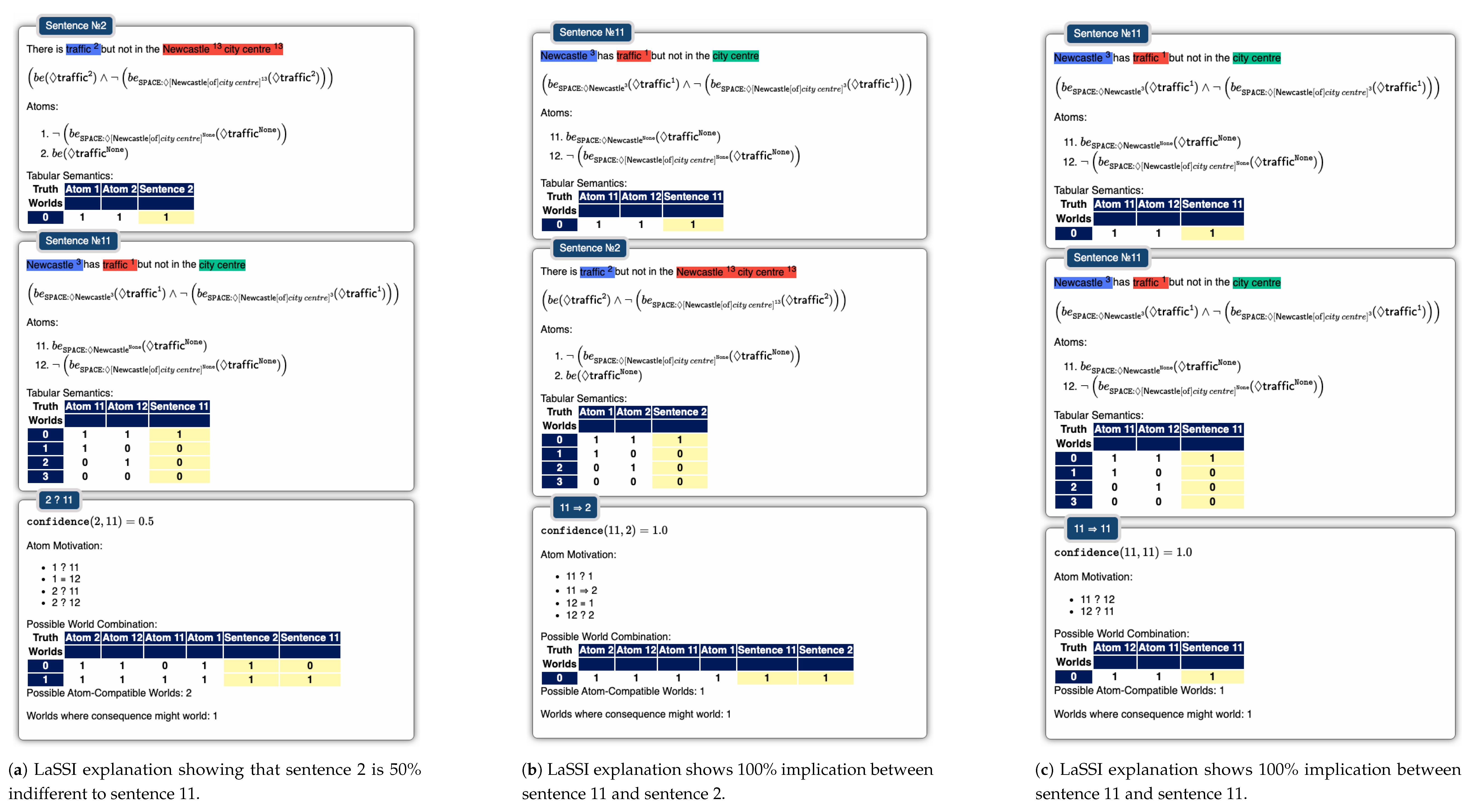
5.3.5. Final Considerations
Table 12 summarises the findings from our previous evaluation: despite our proposed methodology not providing intuitive ways to visualise the derivations leading to the classification outcome, our approach meets all of the aforementioned correctness requirements. Future works will then postulate improved ways to better visualise the classification outcomes similarly to SHAP and LIME explainers.
Given that current state-of-the-art explainers still heavily rely on training another model to derive correlations between input and output data. Consequently, minor differences in the data sampling strategies might produce highly dissimilar explanations even for closely related data points [103]. Most importantly, it is widely known that both LIME and SHAP explainers can be easily manipulated to hide evident biases from the data [104]. As any learning process naturally introduces biases when learning, more rigid control through rule-based mechanisms, such as the ones presented in this paper, should be used to mitigate such effects.
6. Conclusions and Future Works
The proposed LaSSI offers hybrid explainability within an NLP pipeline, which generates logical representations for simple and factoid sentences in a manner based on common sense and knowledge-based networks. Preliminary results suggest the practicality of MG rewriting combining dependency parsing, graph rewriting, and MEU recognition, as well as semantic post-processing operations. We show that, through exploiting a curated KB including both common-sense knowledge (ABox) and rewriting rules (TBox), we can easily capture the essence of similar sentences while remarking on the limitations of the existing state-of-the-art approaches in doing so. Preliminary experiments suggest the inability of transformers to solve problems as closed Boolean expressions expressed in natural language and to reason paraconsistently when using cosine similarity metrics [52]. Compared with pre-trained language models, we showcased their inability to fully capture deep sentence understanding after training over large corpora, even for short factoid sentences. As the comparison in resource usage and running time was disproportionate for these competitors, it would be interesting to provide comparisons with other lightweight NLP methods, which we intend to consider in our future work.
At present, in all the sentences in our dataset, the entities only have at most one preposition contained within the properties; thus, in future datasets, we may include more than one. As we have kept the case properties stored in a key–value pair, where the key indicates the float position within the wider sentence, we could eventually determine “complex prepositions”, formed by combining two or more simple prepositions, within a given sentence. As we intend to test this pipeline on a large scale using real-world crawled data, future works will aim to further improve the presented results regarding this pipeline by first analysing the remaining sentences from ConceptNet, and then attempting to analyse other, more realistic scenarios. Future work will extend to a more diverse range of datasets: given that we are challenging a three-way classification distinguishing between logical implication, indifference, and inconsistency for the first time, as they stand, currently available datasets are unsuitable to test our system under our premises. In particular, we need to completely re-annotate these datasets to encompass the three-fold classification. Meanwhile, to capture more complex sentences, we would need to substantially extend our knowledge base, Parmenides, to cover richer semantic information to capture more complex sentence structures. In future work, we will also consider the possibility of bridging abductive reasoning [18], allowing for rule generalisation, as well as adopting relational learning algorithms, enabling learning over dirty data without cleaning [13,20]. To the best of our knowledge, neither abductive reasoning nor relational learning mechanisms provide learning capabilities over logical formulae potentially containing negations: this might be risky, as it could lead to the explosion problem as well as the derivation of unlikely conclusions over probabilistic data. In future works, we will thus consider integrating such approaches with the paraconsistency capabilities exploited in this study, as well as considering whether a rule-based approach can be used to minimise the effects of semantic leakage problem [51].
As highlighted in the experiments, the meuDB generation step was detrimental to the running time of our pipeline, although once it is generated, the running times significantly decrease. Therefore, further investigations will be performed to reduce the time complexity through a better algorithm, thus ensuring that the LaSSI pipeline is as efficient as possible in the future.
Multidimensional scaling is a well-known methodology for representing distances between pairs of objects embedded as points into Euclidean space [105,106], allowing for the derivation of object embeddings given their pairwise distances. Despite the existence of non-metric solutions [107,108], none of these approaches consider arbitrary divergence functions supporting neither the triangular inequality nor the symmetry requirement, as is the case for the confidence metric used in this paper. The possibility of finding such a technique can be expected to streamline the retrieval of similar constituents within the expansion phase by exploiting kNN queries [109], which can be further streamlined using vector databases and vector-driven indexing techniques [110].
Finally, we can see that deep semantic rewriting cannot be encompassed by the latest GQL standards [68], nor generalised graphs [65], as both are context-free languages [111] that cannot take into account the contextual information that can be only derived through semantic information. As these rewriting phases are not driven by FOL inferences, the inference step boils down to querying a KB to disambiguate the sentence context and semantics; however, most human languages are context-sensitive. This leads to the postulation that further automating and streamlining the rewriting steps detailed in Section 3.2.2, Section 3.2.3, and Section 3.2.4 will require the definition of a context-sensitive query language, which is currently missing from the existing database literature. All of the remaining rewriting steps were encoded using context-free languages. In future works, we will investigate the appropriateness of this language and whether it can be characterised through a straightforward algorithmic extension of GGG.
Author Contributions
Conceptualisation, G.B.; methodology, O.R.F. and G.B.; software, O.R.F. and G.B; validation, O.R.F.; formal analysis, O.R.F.; investigation, O.R.F. and G.B.; resources, G.B.; data curation, O.R.F.; writing—original draft preparation, O.R.F.; writing—review and editing, O.R.F. and G.B.; visualisation, O.R.F.; supervision, G.B. and G.M.; project administration, G.B.; funding acquisition, G.B. All authors have read and agreed to the published version of the manuscript.
Funding
O.R.F.’s research is sponsored by a UK EPSRC PhD Studentship.
Institutional Review Board Statement
Not applicable.
Informed Consent Statement
Not applicable.
Data Availability Statement
The dataset is publicly available at https://osf.io/g5k9q/ (Accessed on 1 April 2025). The repository is available through GitHub (https://github.com/LogDS/LaSSI, Accessed on 28 April 2025).
Acknowledgments
The authors thank Tom McCone for English editing.
Conflicts of Interest
The authors declare no conflicts of interest.
Abbreviations
The following abbreviations are used in this manuscript:
Appendix A. Generation of SetOfSingletons
Appendix A.1. Multi-Word Entities
Compound types are labelled as a type GROUPING. There are two scenarios where compound edges present themselves: first, in a chain , or second, a parent node with multiple children directly descending from it, (Newcastle city centre from Figure A1). To detect these structures, we use DFS, as entities that may have children that present extra information to their parents should be identified before the resolution of the parents. In the pipeline, these edges are removed, with the children either appended to the parent node’s name or added as an extra property of the parent. These can be further refined to separate the main entity from any associated specification (Appendix A.2.1).
Figure A1.
GGG output for “Traffic is flowing in Newcastle city centre, on Saturdays”.
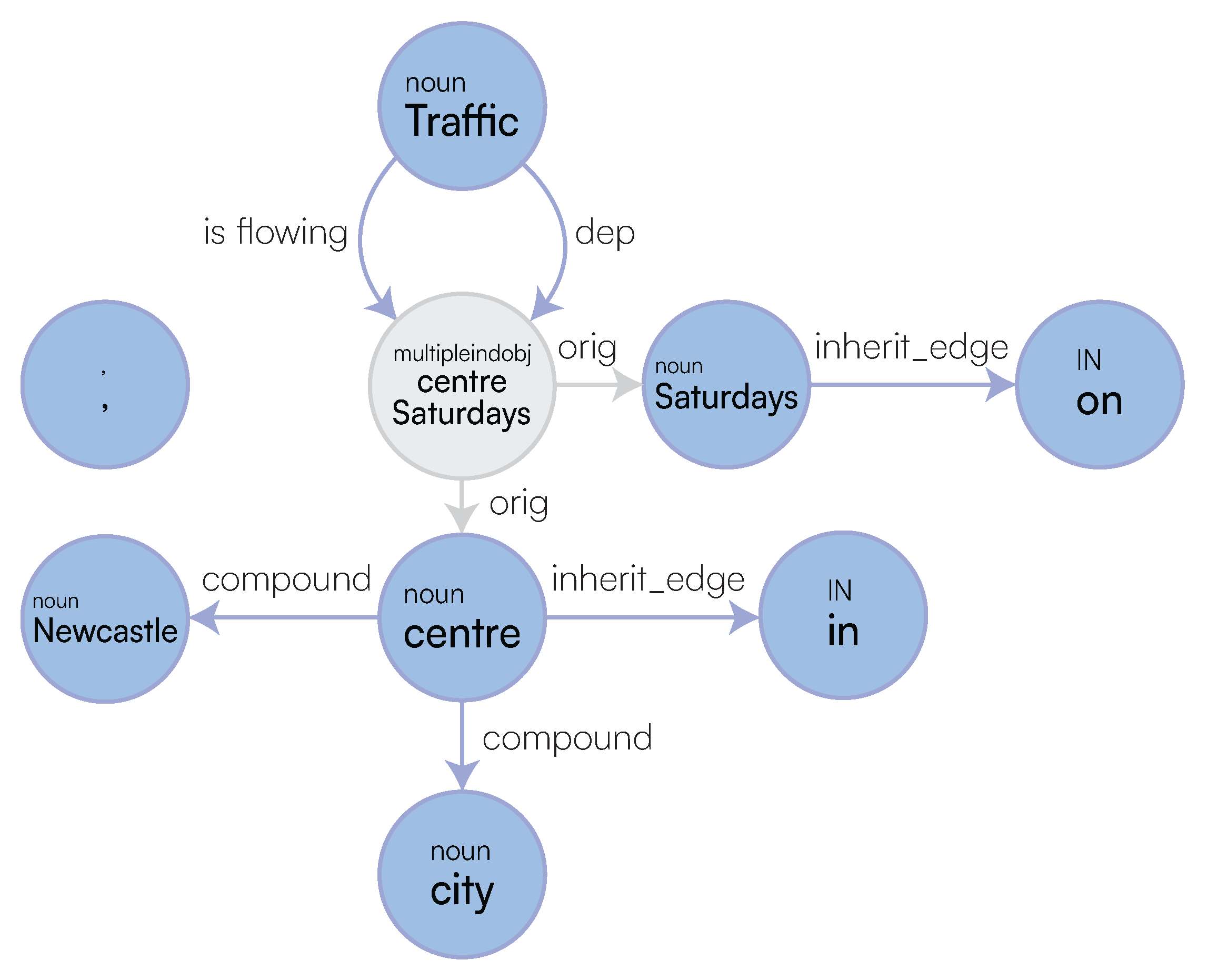
Example A1.
Looking at the second case, we can focus on “Newcastle city centre”, which has edges . Here,Newcastlecrucially needs to be resolved, to identify it is aGeoPolitical Entity (GPE)for when we merge all the Singletons in Algorithm 1.
Appendix A.2. Multiple Logical Functions
Concerning the detection of multiple logical functions, Figure A1 has just one sentence with “is flowing” as a verb, where multiple logical functions have the nodes “centre” and “Saturdays” as entry points and ancestors. The node centre Saturdays would become a SetOfSingletons with entities Newcastle and Saturdays. As we have a node with compound edges in Figure A1, these are resolved into one Singleton per Example A1: Newcastle[extra:city centre]. Finally, we create our new logical relationships: is flowing(traffic, Newcastle[extra:city centre]) and dep(traffic, Newcastle[extra:city centre]).
Appendix A.2.1. Handling Extras
When dealing with multi-word entities, we must identify whether a subset of these words acts as a specification (extra) to the primary entity of interest or whether it should be treated as a single entity. For example, “Newcastle upon Tyne” would be represented as one Singleton with no extra property, whereas “Newcastle city centre” has the core entity “Newcastle” and an extra “city centre”.
To derive which part of the multi-named entity provides a specification for the main entity, we use Algorithm 1. The input takes a node, which is the SetOfSingletons to be resolved, and the meu_db referring to the specific sentence of interest. The entities from the given SetOfSingletons are first sorted by the position of each node occurring within the full text, and a list of alternative representations is created from the power set of its associated entities from which Singletons and empty sets are removed. For example, given an array of three elements , our layered_alternatives from Line 5 are .
Example A2
(Example A1 cont.). For “Newcastle city centre”, we would obtain , representing all possible combinations of each givenSingletonwithin theSetOfSingletonsto extract theextrafrom the main entity.
We based our inference on a type hierarchy to differentiate between the components providing the specification (extra) to the main entity. The hierarchy of types seen in use on Line 9 employs a Most Specific Type (MST) function to return a Specific Type (ST) from a curated entity-type hierarchy as follows: VERB GPELOC(ation) ORGNOUNENTITY ADJECTIVE. If none of these are met, then the type is set to None. This is updated from our previous pipeline so that VERB is now the most specific type. Adjectives are also captured, as these were missing from the previous hierarchy.
Lastly, we look through the meuDB, comparing the minimum and maximum values of the given alternative for a corresponding match that has the highest confidence value (Line 10). These confidence scores lead to how we calculate which alternative should be used for resolving later in our Singleton (Line 12). We check for whether the current candidate in the loop has a greater confidence score than the total confidence score, which is calculated from the product of all confidence scores within the entities.
Appendix B. Recursive Sentence Rewriting
We now describe in greater detail any subroutine required by Algorithm 2 to derive further subsequent computational steps.
Appendix B.1. Promoting Edges to Binary/Unary Relationships
Algorithm A1 collects all the appropriate edges to be considered when creating the kernel, and ensures that all edge labels to be considered are verbs while labels that are not verbs are disregarded. The first step in creating these kernels is obtaining all the appropriate edges and determining which nodes within those edges are already roots, or should be considered if they are not already. This is presented in Line 1. Edges that are labelled with `dep’ are skipped in Line 7 as, for this type of edge, it is `impossible to determine a more precise relation’ [112], and they can therefore be ignored. Next, we check every edge label for prototypical prepositions, retrieved from our ontology in Line 3, which determines target nodes to be roots which are not already handled by dependency parsing. These prototypical prepositions are a single word (a preposition) that precedes a noun phrase complement, which expresses spatial relations [113]; for example: “the mouse is eatenby the cat” or “charactersin movies”. We check whether a edge contains a prototypical preposition in Line 10: we want to determine whether the preposition is contained within a wider edge label, but is not exactly equal to it; for example, if we had the label “to steal”, this contains “to”, so it would return true. However, if we had “like”, this is exactly equal to a preposition and, therefore, false would be returned. We also check for when the target does not contain a case property as, if we imply that a target with a case property is a sub-sentence, then we may lose additional information necessary for the logical rewriting phase in Section 3.2.3. We also perform an additional check for whether the edge label ends with “ing” and does not contain an auxiliary as a condition, in order to accept a true state for a prototypical preposition. We carry out this process such that sub-sentences can still be captured when a preposition is not contained within the full text, but still introduced by a verb in its gerund form (-ing). We ensure that this does not contain an auxiliary, such that we do not incorrectly consider that a new sentence is being introduced.
| Algorithm A1 Edges collected from our a priori phase need to be analysed to ensure that they are all relevant and structured correctly, such that our kernel best represents the given full text. This function checks for prototypical prepositions within edge labels, in order to possibly rewrite targets of a number of edges. |
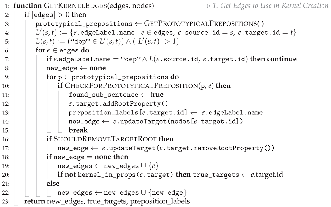 |
If we find a preposition, we add a root property to the target node of the given edge and map the target ID to the full edge label name in a prepositions list, which is to be used when determining which edge to use when creating the sentence in Algorithm A3.
There might be situations where roots are incorrectly identified, which is reflected in Line 16. We check the following: if we have not found a preposition in the current edge label, the edge label is a verb, the source is a root, and the target is not an existential variable. If these conditions are all true, then the target’s root property (if present) is removed. We are removing something that is incorrectly recognised as a root; however, this does not affect verbs as in Algorithm A2, and Line 5 will always return true if the given entity is a verb regardless of whether it contains a root property.
Appendix B.2. Identifying the Clause Node Entry Points
Now that we have a list of all edges that should be considered for our given full text, we need to find the IDs of the nodes that should be considered roots from which we generate all kernels. For this purpose, Algorithm A2 iterates over each source and target node within every edge collected in the previous step (Algorithm A1). Then, we filter each node by checking if they have a root property and are not contained within the list of true targets, in order to mitigate the chance of duplicate root IDs being added to filtered_nodes on Line 5. We also perform an additional check for whether the node is a SetOfSingletons, and remove any node from the list that may be a child of the SetOfSingletons, as it would be incorrect to consider them roots given that they are contained within the parent of the SetOfSingletons.
| Algorithm A2 To properly encompass the recursive nature of the sentence, we find the root IDs within the given edges in topological order, ensuring that we maintain structural understanding when rewriting the sentence. (Algorithm 2 cont.) |
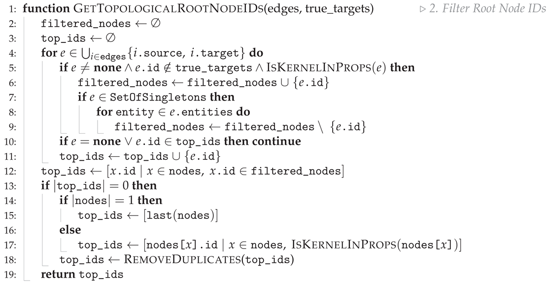 |
With the filtered_nodes collected, we need to sort them in topological order. In this way, when creating our logical representation, the structure is compliant with the original representation of the full text. As we have performed a topological sort on the list of nodes when first parsing the GSM to generate a graph, we create a list of top_ids in Line 12. If we have not found any root nodes based on the filtering performed, then, if only one node remains, this becomes our root node; otherwise, we collect all nodes that have a root property as a fallback.
Appendix B.3. Generating Binary Relationships (Kernels)
To create our intermediate binary relationships, Algorithm A3 retrieves the node from the passed root_id (our n in Algorithm 2), and check whether we have any edges to use in rewriting. If we do not have any edges and the node is a verb, we create an `edge kernel’ on Line 5; as an example, if we had the node `work’ with no other edges, then we return the kernel work(?, None), as we have no further information at this stage. If it is not a verb and there are no edges, then we simply return the node as we cannot perform any rewriting.
If these conditions are not met, then we assign our kernel, whereby we find the source, target, and edge label to be used (as detailed in Algorithm A4). From this returned kernel, we create a list of kernel_nodes, which are the nodes to be considered before adding to the properties of the kernel. Here, if a property to be added is in the kernel_nodes, it should be ignored as the information is already contained in the entire kernel. Therefore, we call a function to `analyse’ the source and target in Line 9, which adds the source and target to kernel_nodes.
Next, we iterate over each edge e, and add the source and target nodes of each e to properties (Line 12). If a given e has an edge label equal to `acl_relcl’, `nmod’, `nmod_poss’, then we rewrite this edge as a kernel within a Singleton (Line 15) and add the entire edge to the properties, to later be rewritten in Algorithm A5. If the edge label is `acl_relcl’, then we append this to the acl_map, used in Algorithm 2, in Line 23.
While iterating, we check in Line 17 for cases where e’s properties necessitate the creation another kernel from the edges. If e is a verb and not already in the kernel_nodes, we use this edge in the next iteration within Algorithm A3 using the same root node; in particular, previousKernel is assigned to the current kernel at Line 27. We then check for this in Line 18, where we compare the current and previous kernels in order to determine whether the previous kernel should become the root or be added as a property; this is determined by the positions of each (Line 20).
| Algorithm A3 Construct final relationship (kernel) (Algorithm 2 cont.) |
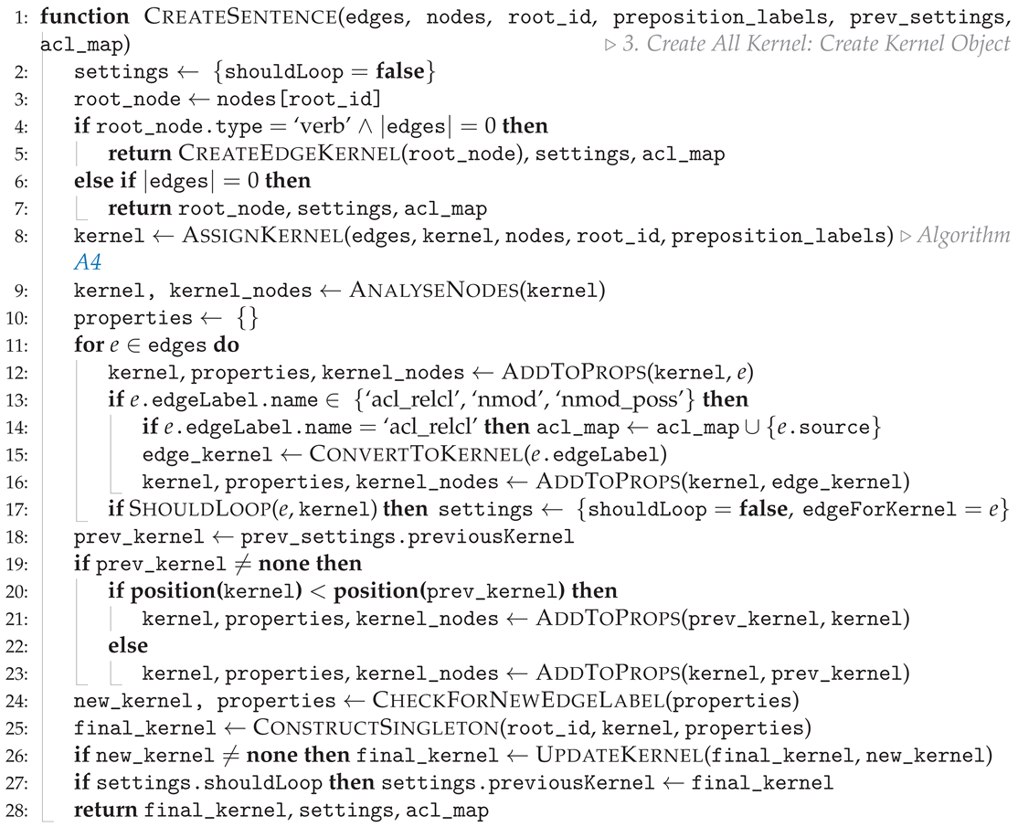 |
Appendix B.3.1. Kernel Assignment
To assign our kernel, Algorithm A4 first needs to determine which edge applies to the current kernel in Line 3, iterating over all the edges to find our chosen_edge. We then iterate again over the edges and, once we reach either our chosen edge or a verb when no chosen edge is found, we determine the attributes of our kernel. As long as our edge label is a verb, it remains the same; otherwise, we use the source of the current e. According to the condition on Line 6, our source becomes an existential (Line 10); otherwise, it remains as the source of e. We then construct our kernel and check whether the edge label is a transitive verb or not (Section 2.3) and, if it is not, then we remove the target as it reflects the direct object.
If no kernel can be constructed, we look for an existential in Line 15 by checking the source and target for existential properties. If we still cannot construct a kernel (i.e., no existential is found); then, we forcefully create the existential by looking for a verb within the list of nodes in Line 17.
At this stage, we check whether a case property is contained within the source or target and, if so, we remove the node (which is later appended as a property of the kernel). If the source is removed, it is replaced with an existential; if the target is removed, it is replaced with none. However, if our target is a SetOfSingletons, then we look for a valid target within the entities target, where we use the first occurring element by its position in the entities and append the rest of the entities as properties (Line 23).
| Algorithm A4 Given a list of edges, we find the most relevant edge (using a set of rules narrated in the text) that should be used as our kernel. (Algorithm A3 cont.) |
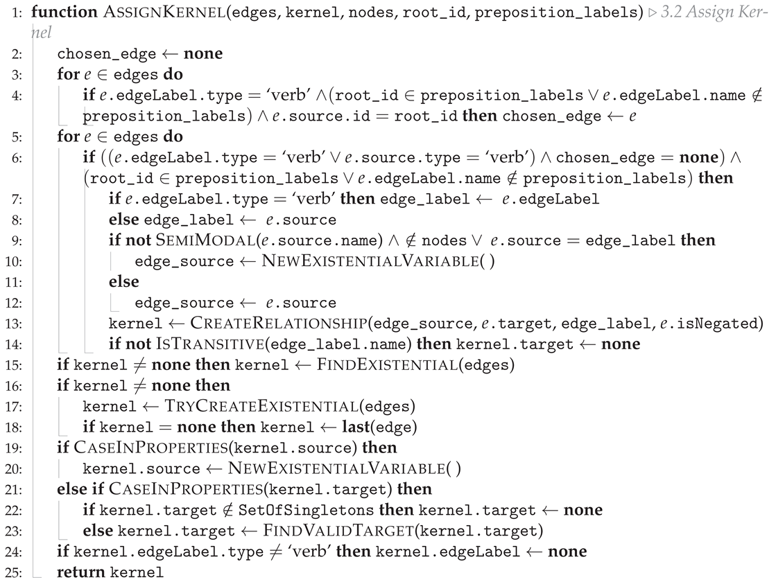 |
Appendix C. Rewriting Semantics for Logical Function Rules in Parmenides
Algorithm 3 in Section 3.2.3 shows how all the properties for a given kernel are rewritten and ensures recursiveness for any given kernel by ensuring that properties of properties are accounted for. Each key (typically) contains an array of entities, where n is each entity in the key iterated over in Line 7. If n is a Singleton, we check that this contains a kernel and rewrite it accordingly; if the node is an nmod or nmod_poss, then we perform an additional check to determine whether the rewritten property can be replaced within the source or target of the current kernel (k). In Line 4, we perform a check to determine whether the key is extra, which signifies that the current properties have already been logically rewritten and, therefore, can be skipped. In Line 25, we create a new SetOfSingletons so long as the function in Line 21 returns a key_to_use. This will have an ID matching prop_node, and contain one element (which is prop_node) and a type (which is the key from Line 3). For example, the sentence: “There is traffic but not in the Newcastle city centre” is initially be(traffic, ?)[(AND:NOT(Newcastle[(extra:city centre), (6:in), (det:the)]))]; therefore, through Lines 19–23, as (6:in) is contained within Newcastle, this is rewritten as
be(traffic, ?)[(SPACE:AND(NOT(Newcastle[(extra:city centre), (type:stay in place), (det:the)])))]
Algorithm A5 then rewrites a matched kernel according to the ontology information, as per the example listed in Figure 9c. The algorithm returns properties with the (potentially) new `type key’—referring to the logical rewriting—which is then added to the kernel. The parameters passed include the entire kernel, the initial_node (being the node to be rewritten), properties (which is the set of properties to be added to the entire kernel), has_nmod (a Boolean from Line 10 in Algorithm 3), and return_key (used for rewriting SetOfSingletons). Additional rules are also included to deal with swapping the target with the properties, as discussed in more detail in Section ??.
| Algorithm A5 Given a node, taken from our kernel, we try to match a rule from our Parmenides ontology. From this rule we get the type which determines the rewriting function, that should be applied to the given node. This function also determines whether the rewriting should be added to the properties of the given Singleton, or to the entire kernel. |
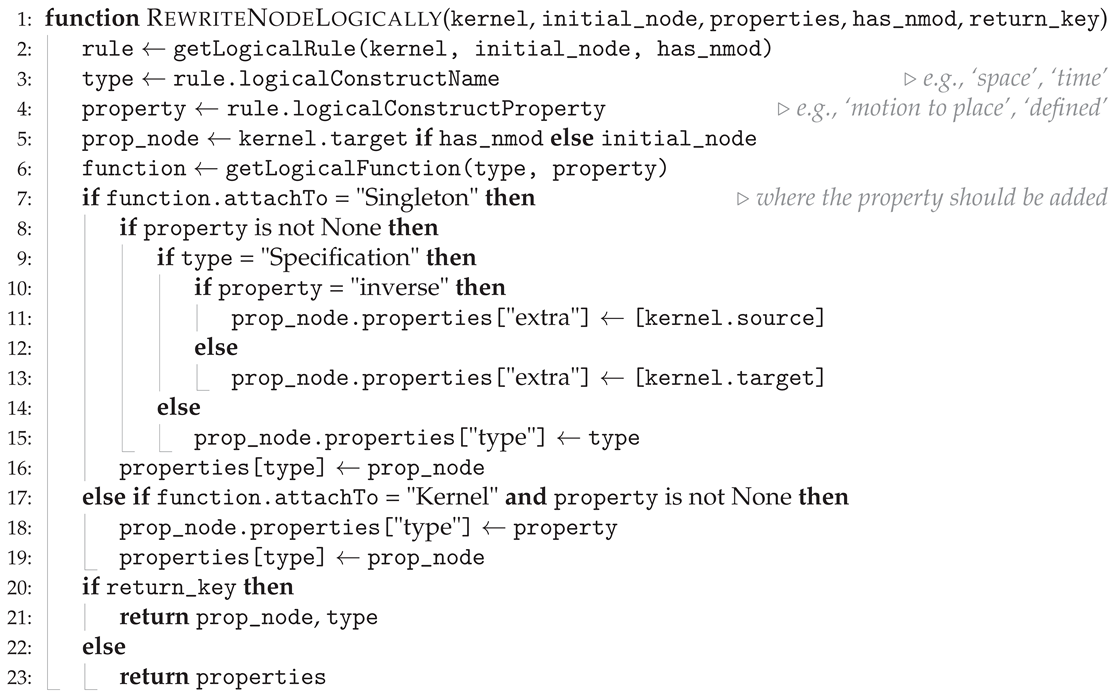 |
Appendix D. Classical Semantics, Bag Semantics, and Relational Algebra
Appendix D.1. Enumerating the Set of Possible Worlds Holding for a Formula
For relational algebra, we denote × as the cross product, ⋈ as the natural equi-join, as the select/filter operator over a binary predicate P, and as the projection operator selecting only the attributes appearing in L. We define as the non-classical relational algebra operator extending the relational table T with a new attribute A while extending each tuple via f as . Given a logical formula and some truth assignments to logical predicates through a function , we use to denote the valuation function computed over via the truth assignments in .
After determining all the binary or unary predicates associated to a Logical Representation (LR) of a factoid sentence s, we derive a truth table for , represented as a relational table , by assuming each proposition to be completely independent of the others without any further background knowledge.
Appendix D.2. Knowledge-Based Driven Propositional Semantics
Following in the footsteps of our previous research [14], we derive the following conditions through which we discretise the notion of logical implication between propositions and their properties:
Definition A3.
(Multi-Valued Semantics). Given a KB , we say that two propositions or properties are equivalent () if either they satisfy the structural equivalence ≡ formally defined as Leibniz equivalence [114], or if they appear within a transitive closure of equivalence relationships in . We also say that these are inconsistent () if either one of the two is a negation and its argument is Leibniz equivalent to the other or, after a transitive closure of equivalence or logical implications, we derive that one argument is inconsistent in . Then, we distinguish multiple types of logical implications by considering the structure of the proposition extended with data properties:
- :
- If we lose specificity due to some missing copula information.
- :
- By interpreting a missing value from one of the property arguments as missing information entailing any possible value for this field, whether the right element is a non-missing value.
- :
- If we interpret the second object as a specific instance of the first one.
- ↠:
- A general implication state that cannot be easily categorised into any of the former cases while including any of them.
If none of the above applies, then we state that the two propositions or properties are indifferent, and we denote them with ω. We denote any generic implication relationship as .
Appendix D.2.1. Multi-Valued Term Equivalence
Please observe that, in contrast to the standard logic literature, we also consider the negation of terms—implicitly entailing any term being different from the one specified. This shorthand is required, as human language not only expresses negations over entire propositions or formulae, but also over single terms.
When the assessment of multi-valued semantics between two items a and b is determined through a KB , we denote the outcome of such comparison as . In the forthcoming steps, we provide the definitions for the notion of equivalence derivable from the analysis of the structural properties of the propositions and their terms through the KB values given above. The transform when negated function implements the intended semantics of the negation of a multi-valued semantics comparison value: becomes and vice versa, while all other remaining cases are mapped to (as the negation of an implication does not necessarily entail non-implication, and no further information can be derived). The following definition offers an initial definition of term equivalence encompassing the name associated with it, potential specifications associated with them, as well as adjectives generally referred to as copulae:
Definition A4
(Term Equivalence). Given a KB of interest, we denote the discrete notion of term equivalence as follows:
where we use c as a shorthand for the comparison between copulae occurring within flipped terms , n as a shorthand for the name comparison within terms , s as a shorthand for the specification comparison within terms , and as a shorthand of the comparison between name and specification . Given any of the former symbols x, we denote by the flipped variant of the former where the first and second argument are swapped, while always referring to the same arguments (e.g., ).
Appendix D.2.2. Multi-Valued Proposition Equivalence
First, we can consider the equivalence of propositions by types, while ignoring their property arguments p and : while this boils down to the sole argument’s term equivalence for unary propositions (Equation (A2)), for binary predicates, by implicitly considering them as a functional dependency of the first argument over the second, we consider them according to this priority order (Equation (A3)). In both cases, if the propositions differ in terms of the relationship name, we ignore the comparison with .
Given a set of comparison outcomes S referring to comparison outcomes of terms referring to the same key within a property, we define as the function simplifying the comparison outcomes with the most specific multi-valued equivalence output summarising the evidence collected so far:
We also define another function, , for further summarisation of these considerations across all key values within the same property; the purpose of this function is to provide the general notion of proposition similarity at the level of the properties, where the main differences rely on the order of application of the rules. If both properties have no properties, they are deemed equivalent on those premises:
After this, we can define two functions, summarising the implication relationships within properties p and for the first and second propositions, respectively: considers the verse of the implication from the first term towards the second (Equation (A6)), while considers the inverse order (Equation (A7)):
Given these ancillary definitions, we can now define the concept of discrete equivalence between propositions occurring within the formula:
Definition A5.
Given a KB and two propositions a and b, where the first is associated with a property p and the second with a property , we can define the following discrete equivalence function:
where γ is shorthand for the comparison outcome between either binary () or unary () propositions, f is shorthand for the comparison of the first argument considered as a term (), c is a comparison of the first arguments’ copulae if occurring (), and κ summarises the comparison between the first proposition’s properties with the one of the second (), while flips this comparison ().
Appendix E. Proofs
Proof (for Lemma 11).
Given a binary relationship , symmetry is a property of ℜ; that is, if x and y are related in either direction, then x and y are equivalent. Formally, due to the commutative property of the dot product, [?].
□
Proof (for Lemma 12).
If B implies A under a symmetric metric , then A also implies B. This is because the similarity value remains the same regardless of the order of arguments. Formally,
□
Proof (for Lemma 13).
- ⇒
- Left to right: If two equations are the same, they will have the same set of the possible worlds. Given this, their intersection will be always equivalent to one of the two sets, from which it can be derived that the support of either of the two formulas is always true.
- ⇐
- Right to left: When the confidence is 1, then by definition, both the numerator and denominator are of the same size. Therefore, and . By the commutativity of the intersection, we then derive that are of the same size and represent the same set. Thus, it holds that .
□
Proof (for Corollary 14).
The following notation implies that, if there exists x that belongs to and not to , then their intersection size will be less than the size of A and, if has less items then , then it follows that B contains elements not occurring in A:
Then, we want to characterise the logical formula supporting a set of elements belonging to A but not to B. We can derive this from the bag semantics of our logical operators, inferring that the below condition holds when A does not necessarily imply B:
∴ when A holds B does not necessarily hold. □
References
- Zhang, T.; et al. GAIA - A Multi-media Multi-lingual Knowledge Extraction and Hypothesis Generation System. In Proceedings of the Proceedings of the 2018 Text Analysis Conference, TAC 2018, Gaithersburg, Maryland, USA, November 13-14, 2018. NIST, 2018.
- Speer, R.; Chin, J.; Havasi, C. ConceptNet 5.5: An Open Multilingual Graph of General Knowledge. In Proceedings of the Proceedings of the Thirty-First AAAI Conference on Artificial Intelligence, February 4-9, 2017, San Francisco, California, USA; Singh, S.; Markovitch, S., Eds. AAAI Press, 2017, pp. 4444–4451. [CrossRef]
- Auer, S.; Bizer, C.; Kobilarov, G.; Lehmann, J.; Cyganiak, R.; Ives, Z. DBpedia: A nucleus for a web of open data. In Proceedings of the Proceedings of the 6th International The Semantic Web and 2nd Asian Conference on Asian Semantic Web Conference, Berlin, Heidelberg, 2007; ISWC’07/ASWC’07, p. 722–735.
- Mendes, P.; Jakob, M.; Bizer, C. DBpedia: A Multilingual Cross-domain Knowledge Base. In Proceedings of the Proceedings of the Eighth International Conference on Language Resources and Evaluation (LREC`12); Calzolari, N.; Choukri, K.; Declerck, T.; Doğan, M.U.; Maegaard, B.; Mariani, J.; Moreno, A.; Odijk, J.; Piperidis, S., Eds., Istanbul, Turkey, 2012; pp. 1813–1817.
- Bergami, G. A framework supporting imprecise queries and data, 2019, [arXiv:cs.DB/1912.12531].
- Talmor, A.; Herzig, J.; Lourie, N.; Berant, J. CommonsenseQA: A Question Answering Challenge Targeting Commonsense Knowledge. In Proceedings of the Proceedings of the 2019 Conference of the North American Chapter of the Association for Computational Linguistics: Human Language Technologies, Volume 1 (Long and Short Papers); Burstein, J.; Doran, C.; Solorio, T., Eds., Minneapolis, Minnesota, 2019; pp. 4149–4158. [CrossRef]
- Kreutz, C.K.; Wolz, M.; Knack, J.; Weyers, B.; Schenkel, R. SchenQL: In-depth analysis of a query language for bibliographic metadata. International Journal on Digital Libraries 2022, 23, 113–132. [CrossRef]
- Li, F.; Jagadish, H.V. NaLIR: An interactive natural language interface for querying relational databases. In Proceedings of the Proceedings of the 2014 ACM SIGMOD International Conference on Management of Data, New York, NY, USA, 2014; SIGMOD ’14, p. 709–712. [CrossRef]
- Tammet, T.; Järv, P.; Verrev, M.; Draheim, D. An Experimental Pipeline for Automated Reasoning in Natural Language (Short Paper). In Proceedings of the Automated Deduction – CADE 29; Pientka, B.; Tinelli, C., Eds., Cham, 2023; pp. 509–521.
- Bao, Q.; Peng, A.Y.; Deng, Z.; Zhong, W.; Gendron, G.; Pistotti, T.; Tan, N.; Young, N.; Chen, Y.; Zhu, Y.; et al. Abstract Meaning Representation-Based Logic-Driven Data Augmentation for Logical Reasoning. In Proceedings of the Findings of the Association for Computational Linguistics: ACL 2024; Ku, L.W.; Martins, A.; Srikumar, V., Eds., Bangkok, Thailand, 2024; pp. 5914–5934. [CrossRef]
- Dallachiesa, M.; Ebaid, A.; Eldawy, A.; Elmagarmid, A.; Ilyas, I.F.; Ouzzani, M.; Tang, N. NADEEF: A commodity data cleaning system. In Proceedings of the Proceedings of the 2013 ACM SIGMOD International Conference on Management of Data, New York, NY, USA, 2013; SIGMOD ’13, p. 541–552.
- Andrzejewski, W.; Bębel, B.; Boiński, P.; Wrembel, R. On tuning parameters guiding similarity computations in a data deduplication pipeline for customers records: Experience from a R&D project. Information Systems 2024, 121, 102323.
- Picado, J.; Davis, J.; Termehchy, A.; Lee, G.Y. Learning Over Dirty Data Without Cleaning. In Proceedings of the Proceedings of the 2020 International Conference on Management of Data, SIGMOD Conference 2020, online conference [Portland, OR, USA], June 14-19, 2020; Maier, D.; Pottinger, R.; Doan, A.; Tan, W.; Alawini, A.; Ngo, H.Q., Eds. ACM, 2020, pp. 1301–1316.
- Bergami, G. A framework supporting imprecise queries and data. CoRR 2019, abs/1912.12531, [1912.12531].
- Virgilio, R.D.; Maccioni, A.; Torlone, R. Approximate querying of RDF graphs via path alignment. Distributed Parallel Databases 2015, 33, 555–581.
- Fox, O.R.; Bergami, G.; Morgan, G. LaSSI: Logical, Structural, and Semantic text Interpretation. In Proceedings of the Database Engineered Applications. Springer, 2025, IDEAS ’24 (in press).
- Wong, P.C.; Whitney, P.; Thomas, J. Visualizing Association Rules for Text Mining. In Proceedings of the Proceedings of the 1999 IEEE Symposium on Information Visualization, USA, 1999; INFOVIS ’99, p. 120.
- Tsamoura, E.; Hospedales, T.; Michael, L. Neural-Symbolic Integration: A Compositional Perspective. Proceedings of the AAAI Conference on Artificial Intelligence 2021, 35, 5051–5060. [CrossRef]
- Raedt, L.D. Logical and Relational Learning; Springer-Verlag Berlin Heidelberg, 2008.
- Picado, J.; Termehchy, A.; Fern, A.; Ataei, P. Logical scalability and efficiency of relational learning algorithms. The VLDB Journal 2019, 28, 147–171. [CrossRef]
- Niles, I.; Pease, A. Towards a standard upper ontology. In Proceedings of the 2nd International Conference on Formal Ontology in Information Systems, FOIS 2001, Ogunquit, Maine, USA, October 17-19, 2001, Proceedings. ACM, 2001, pp. 2–9. [CrossRef]
- Simard, P.Y.; Amershi, S.; Chickering, D.M.; Pelton, A.E.; Ghorashi, S.; Meek, C.; Ramos, G.A.; Suh, J.; Verwey, J.; Wang, M.; et al. Machine Teaching: A New Paradigm for Building Machine Learning Systems. CoRR 2017, abs/1707.06742, [1707.06742].
- Ramos, G.; Meek, C.; Simard, P.; Suh, J.; and, S.G. Interactive machine teaching: A human-centered approach to building machine-learned models. Human–Computer Interaction 2020, 35, 413–451. [CrossRef]
- Mosqueira-Rey, E.; Hernández-Pereira, E.; Alonso-Ríos, D.; Bobes-Bascarán, J.; Fernández-Leal, Á. Human-in-the-loop machine learning: A state of the art. Artificial Intelligence Review 2023, 56, 3005–3054. [CrossRef]
- Seshia, S.A.; Sadigh, D.; Sastry, S.S. Toward verified artificial intelligence. Commun. ACM 2022, 65, 46–55.
- Bergami, G.; Fox, O.R.; Morgan, G., Extracting Specifications through Verified and Explainable AI: Interpretability, Interoperabiliy, and Trade-offs (In Press). In Explainable Artificial Intelligence for Trustworthy Decisions in Smart Applications; Springer; chapter 2.
- Ma, L.; Kang, H.; Yu, G.; Li, Q.; He, Q. Single-Domain Generalized Predictor for Neural Architecture Search System. IEEE Transactions on Computers 2024, 73, 1400–1413. [CrossRef]
- Zini, J.E.; Awad, M. On the Explainability of Natural Language Processing Deep Models. ACM Comput. Surv. 2023, 55, 103:1–103:31. [CrossRef]
- Ayoub, J.; Yang, X.J.; Zhou, F. Combat COVID-19 infodemic using explainable natural language processing models. Information Processing & Management 2021, 58, 102569. [CrossRef]
- Sun, X. Structure Regularization for Structured Prediction. In Proceedings of the Advances in Neural Information Processing Systems 27: Annual Conference on Neural Information Processing Systems 2014, December 8-13 2014, Montreal, Quebec, Canada; Ghahramani, Z.; Welling, M.; Cortes, C.; Lawrence, N.D.; Weinberger, K.Q., Eds., 2014, pp. 2402–2410.
- "Manning, C.; Surdeanu, M.; Bauer, J.; Finkel, J.; Bethard, S.; McClosky, D. The Stanford CoreNLP Natural Language Processing Toolkit. In Proceedings of the Proceedings of 52nd Annual Meeting of the Association for Computational Linguistics: System Demonstrations; Bontcheva, K.; Zhu, J., Eds., Baltimore, Maryland, jun 2014; pp. 55–60. [CrossRef]
- Jurafsky, D.; Martin, J.H. Speech and Language Processing: An Introduction to Natural Language Processing, Computational Linguistics, and Speech Recognition with Language Models, 3rd ed.; 2025. Online manuscript released January 12, 2025.
- Nivre, J.; et al. conj. Available online: https://universaldependencies.org/en/dep/conj.html (accessed on 13.02.2025).
- Nivre, J.; et al. cc. Available online: https://universaldependencies.org/en/dep/cc.html (accessed on 13.02.2025).
- Chen, D.; Manning, C.D. A Fast and Accurate Dependency Parser using Neural Networks. In Proceedings of the Proceedings of the 2014 Conference on Empirical Methods in Natural Language Processing, EMNLP 2014, October 25-29, 2014, Doha, Qatar, A meeting of SIGDAT, a Special Interest Group of the ACL; Moschitti, A.; Pang, B.; Daelemans, W., Eds. ACL, 2014, pp. 740–750. [CrossRef]
- Goodman, J.; Vlachos, A.; Naradowsky, J. Noise reduction and targeted exploration in imitation learning for Abstract Meaning Representation parsing. In Proceedings of the Proceedings of the 54th Annual Meeting of the Association for Computational Linguistics (Volume 1: Long Papers); Erk, K.; Smith, N.A., Eds., Berlin, Germany, 2016; pp. 1–11. [CrossRef]
- Stanford NLP Group. The Stanford Natural Language Processing Group. Available online: https://nlp.stanford.edu/software/lex-parser.shtml (accessed on 24.02.2025).
- Cardona, G. Pāṇini – His Work and its Traditions, 2 ed.; Vol. 1, Motilal Banarsidass: London, 1997.
- Christensen, C.H. Arguments for and against the Idea of Universal Grammar. Leviathan: Interdisciplinary Journal in English 2019, p. 12–28. [CrossRef]
- Hauser, M.D.; Chomsky, N.; Fitch, W.T. The Faculty of Language: What Is It, Who Has It, and How Did It Evolve? Science 2002, 298, 1569–1579, [https://www.science.org/doi/pdf/10.1126/science.298.5598.1569]. [CrossRef]
- Bergami, G., On Nesting Graphs. In A new Nested Graph Model for Data Integration; University of Bologna, Italy; chapter 7, pp. 195–220. PhD thesis.
- Montague, R., ENGLISH AS A FORMAL LANGUAGE. In Logic and philosophy for linguists; De Gruyter Mouton: Berlin, Boston, 1975; pp. 94–121. [CrossRef]
- Montague, R. English as a formal language. In Linguaggi nella Societa e nella Tecnica; Edizioni di Communità: Milan, Italy, 1970; pp. 189–224.
- Dardano, M.; Trifone, P. Italian grammar with linguistics notions (in Italian); Zanichelli: Milan, 2002.
- terdon. terminology - Syntactic analysis in English: Correspondence between Italian complements and English ones. Available online: https://english.stackexchange.com/questions/628592/syntactic-analysis-in-english-correspondence-between-italian-complements-and/628597#628597 (accessed on 10.02.2025).
- Song, K.; Tan, X.; Qin, T.; Lu, J.; Liu, T. MPNet: Masked and Permuted Pre-training for Language Understanding, 2020.
- Liu, Y.; Ott, M.; Goyal, N.; Du, J.; Joshi, M.; Chen, D.; Levy, O.; Lewis, M.; Zettlemoyer, L.; Stoyanov, V. RoBERTa: A Robustly Optimized BERT Pretraining Approach, 2019, [arXiv:cs.CL/1907.11692].
- Wang, W.; Bao, H.; Huang, S.; Dong, L.; Wei, F. MiniLMv2: Multi-Head Self-Attention Relation Distillation for Compressing Pretrained Transformers. In Proceedings of the Findings of the Association for Computational Linguistics: ACL-IJCNLP 2021; Zong, C.; Xia, F.; Li, W.; Navigli, R., Eds., Online, 2021; pp. 2140–2151. [CrossRef]
- Santhanam, K.; Khattab, O.; Saad-Falcon, J.; Potts, C.; Zaharia, M. ColBERTv2: Effective and Efficient Retrieval via Lightweight Late Interaction. In Proceedings of the Proceedings of the 2022 Conference of the North American Chapter of the Association for Computational Linguistics: Human Language Technologies; Carpuat, M.; de Marneffe, M.C.; Meza Ruiz, I.V., Eds., Seattle, United States, 2022; pp. 3715–3734. [CrossRef]
- Vaswani, A.; Shazeer, N.; Parmar, N.; Uszkoreit, J.; Jones, L.; Gomez, A.N.; Kaiser, L.u.; Polosukhin, I. Attention is All you Need. In Proceedings of the Advances in Neural Information Processing Systems; Guyon, I.; Luxburg, U.V.; Bengio, S.; Wallach, H.; Fergus, R.; Vishwanathan, S.; Garnett, R., Eds. Curran Associates, Inc., 2017, Vol. 30.
- Gonen, H.; Blevins, T.; Liu, A.; Zettlemoyer, L.; Smith, N.A. Does Liking Yellow Imply Driving a School Bus? Semantic Leakage in Language Models. In Proceedings of the Proceedings of the 2025 Conference of the Nations of the Americas Chapter of the Association for Computational Linguistics: Human Language Technologies (Volume 1: Long Papers); Chiruzzo, L.; Ritter, A.; Wang, L., Eds., Albuquerque, New Mexico, 2025; pp. 785–798.
- Strobl, L.; Merrill, W.; Weiss, G.; Chiang, D.; Angluin, D. What Formal Languages Can Transformers Express? A Survey. Transactions of the Association for Computational Linguistics 2024, 12, 543–561.
- Manning, C.D.; Raghavan, P.; Schütze, H. Introduction to Information Retrieval; Cambridge University Press, 2008.
- Hicks, M.T.; Humphries, J.; Slater, J. ChatGPT is bullshit. Ethics and Information Technology 2024, 26, 38.
- Bender, E.M.; Gebru, T.; McMillan-Major, A.; Shmitchell, S. On the Dangers of Stochastic Parrots: Can Language Models Be Too Big? In Proceedings of the Proceedings of the 2021 ACM Conference on Fairness, Accountability, and Transparency, New York, NY, USA, 2021; FAccT ’21, p. 610–623.
- Chen, Y.; Wang, D.Z. Knowledge expansion over probabilistic knowledge bases. In Proceedings of the International Conference on Management of Data, SIGMOD 2014, Snowbird, UT, USA, June 22-27, 2014; Dyreson, C.E.; Li, F.; Özsu, M.T., Eds. ACM, 2014, pp. 649–660.
- Kyburg, H.E. Probability and the Logic of Rational Belief; Wesleyan University Press: Middletown, CT, USA, 1961.
- Brown, B. Inconsistency measures and paraconsistent consequence. In Measuring Inconsistency in Information; Grant, J.; Martinez, M.V., Eds.; College Press, 2018; chapter 8, pp. 219–234.
- Graydon, M.S.; Lehman, S.M. Examining Proposed Uses of LLMs to Produce or Assess Assurance Arguments. NTRS - NASA Technical Reports Server.
- Ahlers, D. Assessment of the accuracy of GeoNames gazetteer data. In Proceedings of the Proceedings of the 7th Workshop on Geographic Information Retrieval, New York, NY, USA, 2013; GIR ’13, p. 74–81.
- Chang, A.X.; Manning, C. SUTime: A library for recognizing and normalizing time expressions. In Proceedings of the Proceedings of the Eighth International Conference on Language Resources and Evaluation (LREC`12); Calzolari, N.; Choukri, K.; Declerck, T.; Doğan, M.U.; Maegaard, B.; Mariani, J.; Moreno, A.; Odijk, J.; Piperidis, S., Eds., Istanbul, Turkey, 2012; pp. 3735–3740.
- Qi, P.; Zhang, Y.; Zhang, Y.; Bolton, J.; Manning, C.D. Stanza: A Python Natural Language Processing Toolkit for Many Human Languages. In Proceedings of the Proceedings of the 58th Annual Meeting of the Association for Computational Linguistics: System Demonstrations, 2020.
- Speer, R.; Chin, J.; Havasi, C. ConceptNet 5.5: An open multilingual graph of general knowledge. In Proceedings of the AAAI. AAAI Press, 2017, AAAI’17, p. 4444–4451.
- Group, T.P.G.D. PostgreSQL: Documentation: 17: F.16. fuzzystrmatch — determine string similarities and distanceAppendix F. Additional Supplied Modules and Extensions. Available online: https://www.postgresql.org/docs/current/fuzzystrmatch.html (accessed on 18.02.2025).
- Bergami, G.; Fox, O.R.; Morgan, G. Matching and Rewriting Rules in Object-Oriented Databases. Mathematics 2024, 12. [CrossRef]
- Junghanns, M.; Petermann, A.; Rahm, E. Distributed Grouping of Property Graphs with Gradoop. In Proceedings of the Datenbanksysteme für Business, Technologie und Web (BTW 2017), 17. Fachtagung des GI-Fachbereichs ,,Datenbanken und Informationssysteme" (DBIS), 6.-10. März 2017, Stuttgart, Germany, Proceedings; Mitschang, B.; Nicklas, D.; Leymann, F.; Schöning, H.; Herschel, M.; Teubner, J.; Härder, T.; Kopp, O.; Wieland, M., Eds. GI, 2017, Vol. P-265, LNI, pp. 103–122.
- Bergami, G.; Zegadło, W. Towards a Generalised Semistructured Data Model and Query Language. SIGWEB Newsl. 2023, 2023. [CrossRef]
- Bonifati, A.; Murlak, F.; Ramusat, Y. Transforming Property Graphs, 2024, [arXiv:cs.DB/2406.13062].
- Bergami, G.; Fox, O.R.; Morgan, G. Matching and Rewriting Rules in Object-Oriented Databases. Preprints 2024. [CrossRef]
- 2025, C.U.P..A. Modality: forms - Grammar - Cambridge Dictionary. Available online: https://dictionary.cambridge.org/grammar/british-grammar/modality-forms#:~:text=Dare%2C%20need%2C%20ought%20to%20and%20used%20to%20(semi%2Dmodal%20verbs) (accessed on 17.03.2025).
- Nivre, J.; et al. case. Available online: https://universaldependencies.org/en/dep/case.html (accessed on 05.03.2025).
- Nivre, J.; et al. nmod. Available online: https://universaldependencies.org/en/dep/nmod.html (accessed on 05.03.2025).
- Jatnika, D.; Bijaksana, M.A.; Suryani, A.A. Word2Vec Model Analysis for Semantic Similarities in English Words. In Proceedings of the Enabling Collaboration to Escalate Impact of Research Results for Society: The 4th International Conference on Computer Science and Computational Intelligence, ICCSCI 2019, 12-13 September 2019, Yogyakarta, Indonesia; Budiharto, W., Ed. Elsevier, 2019, Vol. 157, Procedia Computer Science, pp. 160–167. [CrossRef]
- Mikolov, T.; Chen, K.; Corrado, G.; Dean, J. Efficient Estimation of Word Representations in Vector Space. In Proceedings of the 1st International Conference on Learning Representations, ICLR 2013, Scottsdale, Arizona, USA, May 2-4, 2013, Workshop Track Proceedings; Bengio, Y.; LeCun, Y., Eds., 2013.
- Rosenberger, J.; Wolfrum, L.; Weinzierl, S.; Kraus, M.; Zschech, P. CareerBERT: Matching resumes to ESCO jobs in a shared embedding space for generic job recommendations. Expert Systems with Applications 2025, 275, 127043. [CrossRef]
- Liu, H.; Bao, H.; Xu, D. Concept Vector for Similarity Measurement Based on Hierarchical Domain Structure. Comput. Informatics 2011, 30, 881–900.
- Nickel, M.; Kiela, D. Poincaré Embeddings for Learning Hierarchical Representations. In Proceedings of the Advances in Neural Information Processing Systems 30: Annual Conference on Neural Information Processing Systems 2017, December 4-9, 2017, Long Beach, CA, USA; Guyon, I.; von Luxburg, U.; Bengio, S.; Wallach, H.M.; Fergus, R.; Vishwanathan, S.V.N.; Garnett, R., Eds., 2017, pp. 6338–6347.
- Asperti, A.; Ciabattoni, A. Logica ad Informatica.
- Bergami, G. A new Nested Graph Model for Data Integration. PhD thesis, University of Bologna, Italy, 2018. [CrossRef]
- Carnielli, W.; Esteban Coniglio, M. Paraconsistent Logic: Consistency, Contradiction and Negation; Springer: Switzerland, 2016.
- Hinman, P.G. Fundamentals of Mathematical Logic; A K Peters/CRC Press, 2005.
- Hugging Face. sentence-transformers (Sentence Transformers. Available online: https://huggingface.co/sentence-transformers (accessed on 24.02.2025).
- Zaki, M.J.; Meira, Jr, W. Data Mining and Machine Learning: Fundamental Concepts and Algorithms, 2 ed.; Cambridge University Press, 2020.
- Arthur, D.; Vassilvitskii, S. k-means++: The advantages of careful seeding. In Proceedings of the Proceedings of the Eighteenth Annual ACM-SIAM Symposium on Discrete Algorithms, SODA 2007, New Orleans, Louisiana, USA, January 7-9, 2007; Bansal, N.; Pruhs, K.; Stein, C., Eds. SIAM, 2007, pp. 1027–1035.
- Kleene, S.C. Introduction to Metamathematics; P. Noordhoff N.V.: Groningen, 1952.
- Rousseeuw, P.J. Silhouettes: A graphical aid to the interpretation and validation of cluster analysis. Journal of Computational and Applied Mathematics 1987, 20, 53–65. [CrossRef]
- Nguyen, X.V.; Epps, J.; Bailey, J. Information Theoretic Measures for Clusterings Comparison: Variants, Properties, Normalization and Correction for Chance. J. Mach. Learn. Res. 2010, 11, 2837–2854. [CrossRef]
- O’Neil, E.J.; O’Neil, P.E.; Weikum, G. The LRU-K Page Replacement Algorithm For Database Disk Buffering. In Proceedings of the Proceedings of the 1993 ACM SIGMOD International Conference on Management of Data, Washington, DC, USA, May 26-28, 1993; Buneman, P.; Jajodia, S., Eds. ACM Press, 1993, pp. 297–306. [CrossRef]
- Johnson, T.; Shasha, D.E. 2Q: A Low Overhead High Performance Buffer Management Replacement Algorithm. In Proceedings of the VLDB’94, Proceedings of 20th International Conference on Very Large Data Bases, September 12-15, 1994, Santiago de Chile, Chile; Bocca, J.B.; Jarke, M.; Zaniolo, C., Eds. Morgan Kaufmann, 1994, pp. 439–450.
- Harrison, J. Handbook of Practical Logic and Automated Reasoning; Cambridge University Press, 2009.
- Simon, H.A. The Science of Design: Creating the Artificial. Design Issues 1988, 4, 67–82.
- Johannesson, P.; Perjons, E. An Introduction to Design Science; Springer, 2021. [CrossRef]
- Dewi, C.; Tsai, B.J.; Chen, R.C. Shapley Additive Explanations for Text Classification and Sentiment Analysis of Internet Movie Database. In Proceedings of the Recent Challenges in Intelligent Information and Database Systems; Szczerbicki, E.; Wojtkiewicz, K.; Nguyen, S.V.; Pietranik, M.; Krótkiewicz, M., Eds., Singapore, 2022; pp. 69–80.
- Wei, J.; Wang, X.; Schuurmans, D.; Bosma, M.; Ichter, B.; Xia, F.; Chi, E.H.; Le, Q.V.; Zhou, D. Chain-of-Thought Prompting Elicits Reasoning in Large Language Models. In Proceedings of the Advances in Neural Information Processing Systems 35: Annual Conference on Neural Information Processing Systems 2022, NeurIPS 2022, New Orleans, LA, USA, November 28 - December 9, 2022; Koyejo, S.; Mohamed, S.; Agarwal, A.; Belgrave, D.; Cho, K.; Oh, A., Eds., 2022.
- Ribeiro, M.T.; Singh, S.; Guestrin, C. "Why Should I Trust You?": Explaining the Predictions of Any Classifier. In Proceedings of the Proceedings of the 22nd ACM SIGKDD International Conference on Knowledge Discovery and Data Mining, San Francisco, CA, USA, August 13-17, 2016; Krishnapuram, B.; Shah, M.; Smola, A.J.; Aggarwal, C.C.; Shen, D.; Rastogi, R., Eds. ACM, 2016, pp. 1135–1144.
- Ribeiro, M.T.; Singh, S.; Guestrin, C. Anchors: High-Precision Model-Agnostic Explanations. Proceedings of the AAAI Conference on Artificial Intelligence 2018, 32.
- Visani, G.; Bagli, E.; Chesani, F. OptiLIME: Optimized LIME Explanations for Diagnostic Computer Algorithms. In Proceedings of the Proceedings of the CIKM 2020 Workshops co-located with 29th ACM International Conference on Information and Knowledge Management (CIKM 2020), Galway, Ireland, October 19-23, 2020; Conrad, S.; Tiddi, I., Eds. CEUR-WS.org, 2020, Vol. 2699, CEUR Workshop Proceedings.
- Watson, D.S.; O’Hara, J.; Tax, N.; Mudd, R.; Guy, I. Explaining Predictive Uncertainty with Information Theoretic Shapley Values. In Proceedings of the Advances in Neural Information Processing Systems 36: Annual Conference on Neural Information Processing Systems 2023, NeurIPS 2023, New Orleans, LA, USA, December 10 - 16, 2023; Oh, A.; Naumann, T.; Globerson, A.; Saenko, K.; Hardt, M.; Levine, S., Eds., 2023.
- Lundberg, S.M.; Lee, S.I. A unified approach to interpreting model predictions. In Proceedings of the Proceedings of the 31st International Conference on Neural Information Processing Systems, Red Hook, NY, USA, 2017; NIPS’17, p. 4768–4777.
- Bengfort, B.; Bilbro, R.; Ojeda, T. Applied Text Analysis with Python: Enabling Language-Aware Data Products with Machine Learning, 1st ed.; O’Reilly Media, Inc., 2018.
- Sanh, V.; Debut, L.; Chaumond, J.; Wolf, T. DistilBERT, a distilled version of BERT: smaller, faster, cheaper and lighter. CoRR 2019, abs/1910.01108, [1910.01108].
- Bai, J.; Cao, R.; Ma, W.; Shinnou, H. Construction of Domain-Specific DistilBERT Model by Using Fine-Tuning. In Proceedings of the International Conference on Technologies and Applications of Artificial Intelligence, TAAI 2020, Taipei, Taiwan, December 3-5, 2020. IEEE, 2020, pp. 237–241. [CrossRef]
- Crabbé, J.; van der Schaar, M. Evaluating the robustness of interpretability methods through explanation invariance and equivariance. In Proceedings of the Proceedings of the 37th International Conference on Neural Information Processing Systems, Red Hook, NY, USA, 2023; NIPS ’23.
- Slack, D.; Hilgard, S.; Jia, E.; Singh, S.; Lakkaraju, H. Fooling LIME and SHAP: Adversarial Attacks on Post hoc Explanation Methods. In Proceedings of the Proceedings of the AAAI/ACM Conference on AI, Ethics, and Society, New York, NY, USA, 2020; AIES ’20, p. 180–186. [CrossRef]
- Kruskal, J.B.; Wish, M. Multidimensional Scaling; Quantitative Applications in the Social Sciences, SAGE Publications, Inc.
- Mead, A. Review of the Development of Multidimensional Scaling Methods. Journal of the Royal Statistical Society. Series D (The Statistician) 1992, 41, 27–39.
- Agarwal, S.; Wills, J.; Cayton, L.; Lanckriet, G.R.G.; Kriegman, D.J.; Belongie, S.J. Generalized Non-metric Multidimensional Scaling. In Proceedings of the Proceedings of the Eleventh International Conference on Artificial Intelligence and Statistics, AISTATS 2007, San Juan, Puerto Rico, March 21-24, 2007; Meila, M.; Shen, X., Eds. JMLR.org, 2007, Vol. 2, JMLR Proceedings, pp. 11–18.
- Quist, M.; Yona, G. Distributional Scaling: An Algorithm for Structure-Preserving Embedding of Metric and Nonmetric Spaces. J. Mach. Learn. Res. 2004, 5, 399–420.
- Costa, C.F.; Nascimento, M.A.; Schubert, M. Diverse nearest neighbors queries using linear skylines. GeoInformatica 2018, 22, 815–844. [CrossRef]
- Botea, V.; Mallett, D.; Nascimento, M.A.; Sander, J. PIST: An Efficient and Practical Indexing Technique for Historical Spatio-Temporal Point Data. GeoInformatica 2008, 12, 143–168. [CrossRef]
- Hopcroft, J.E.; Ullman, J.D. Introduction to Automata Theory, Languages and Computation; Addison-Wesley, 1979.
- Nivre, J.; et al. dep. Available online: https://universaldependencies.org/en/dep/dep.html (accessed on 27.02.2025).
- Weber, D. English Prepositions in the History of English Grammar Writing. AAA: Arbeiten aus Anglistik und Amerikanistik 2012, 37, 227–243.
- Asperti, A.; Ricciotti, W.; Sacerdoti Coen, C. Matita Tutorial. Journal of Formalized Reasoning 2014, 7, 91–199. [CrossRef]
- Defays, D. An efficient algorithm for a complete link method. The Computer Journal 1977, 20, 364–366, [https://academic.oup.com/comjnl/article-pdf/20/4/364/1108735/200364.pdf]. [CrossRef]
- Nielsen, F., Hierarchical Clustering. In Introduction to HPC with MPI for Data Science; Springer International Publishing: Cham, 2016; pp. 195–211. [CrossRef]
- Partitioning Around Medoids (Program PAM). In Finding Groups in Data; John Wiley & Sons, Ltd, 1990; chapter 2, pp. 68–125, [https://onlinelibrary.wiley.com/doi/pdf/10.1002/9780470316801.ch2]. [CrossRef]
- Mathew, J.; Kshirsagar, R.; Abidin, D.; Griffin, J.; Kanarachos, S.; James, J.; Alamaniotis, M.; Fitzpatrick, M. A comparison of machine learning methods to classify radioactive elements using prompt-gamma-ray neutron activation data. [CrossRef]
- Nivre, J.; et al. English Dependency Relations. Available online: https://universaldependencies.org/en/dep/ (accessed on 24.02.2025).
| 1 | The previous phase provided a preliminary rewriting, where a new relationship is derived from each verb occurring within the pipeline and connecting the agents performing and receiving the action; information concerning additional entities and pronouns occurring within the sentence is collected among the properties associated with the relationship. |
| 2 | See Appendix D.2 for further details on this notation. |
Figure 1.
Visualisation of the differences between POS tagging, AMR graphs, and UDs, providing more explicit relationships between words. AMRs were generated through AMREager (https://bollin.inf.ed.ac.uk, Accessed on 24 April 2025), while UDs were generated using StanfordNLP [35]. Graphs are highlighted to word correspondences, represented as graph nodes+.
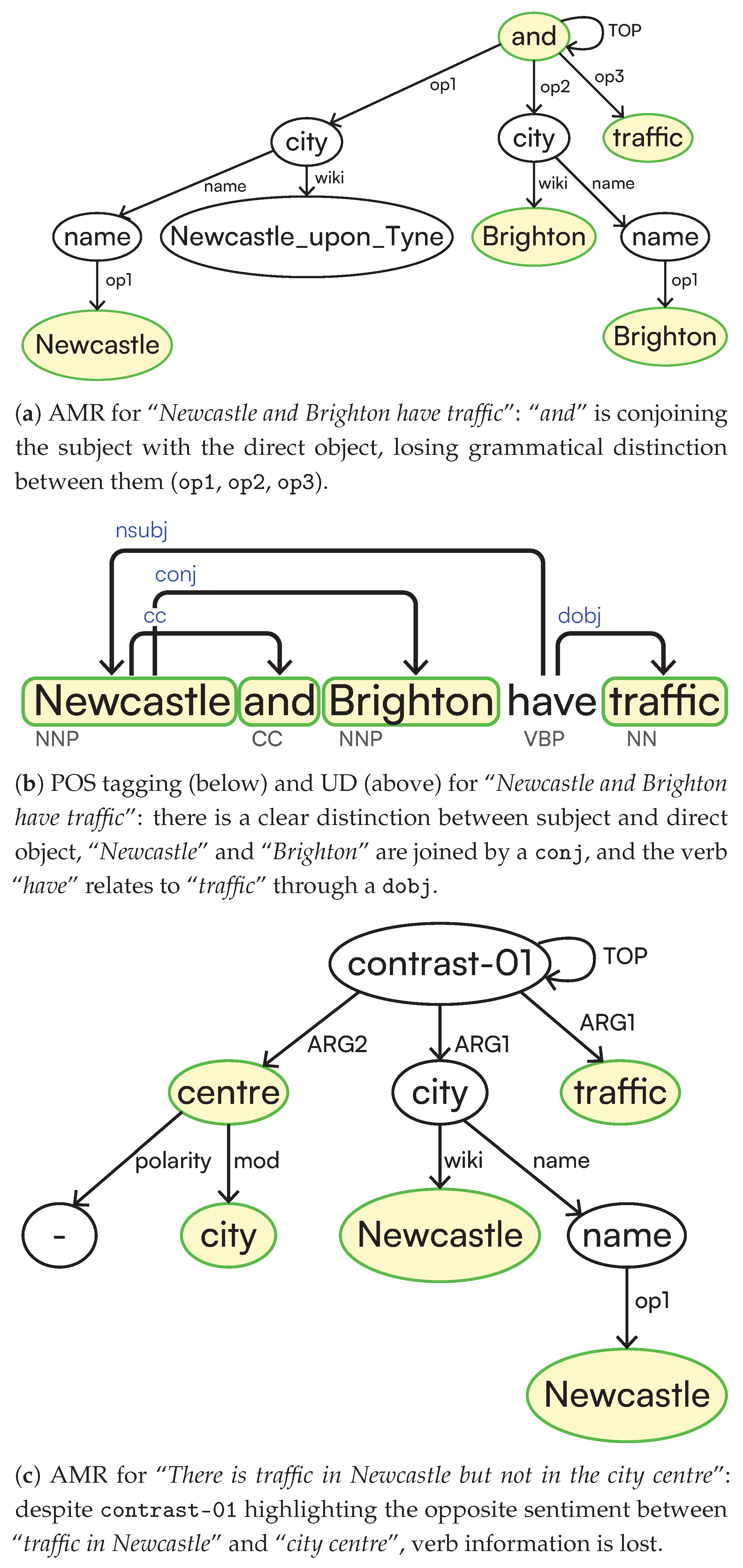
Figure 2.
Example of a recursive sentence, highlighted with coloured bounding boxes [41].
Figure 2.
Example of a recursive sentence, highlighted with coloured bounding boxes [41].

Figure 6.
Continuing the example from Figure 5, we display how SetOfSingletons with type GROUPING are rewritten into Singletons with anextra property, modifying the main entity with additional spatial information. Line numbers refer to distinct subsequent phases from Algorithm 1.
Figure 6.
Continuing the example from Figure 5, we display how SetOfSingletons with type GROUPING are rewritten into Singletons with anextra property, modifying the main entity with additional spatial information. Line numbers refer to distinct subsequent phases from Algorithm 1.
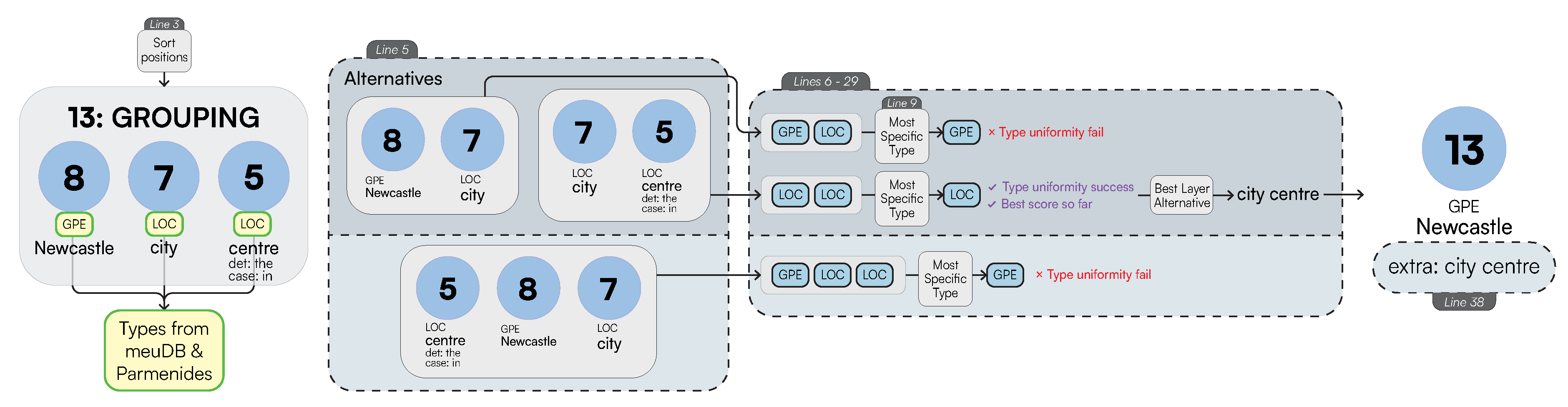
Figure 7.
Transforming the GGG rewriting of a UD graph into a graph Intermediate Representation for “Newcastle and Brighton have traffic”.
Figure 7.
Transforming the GGG rewriting of a UD graph into a graph Intermediate Representation for “Newcastle and Brighton have traffic”.
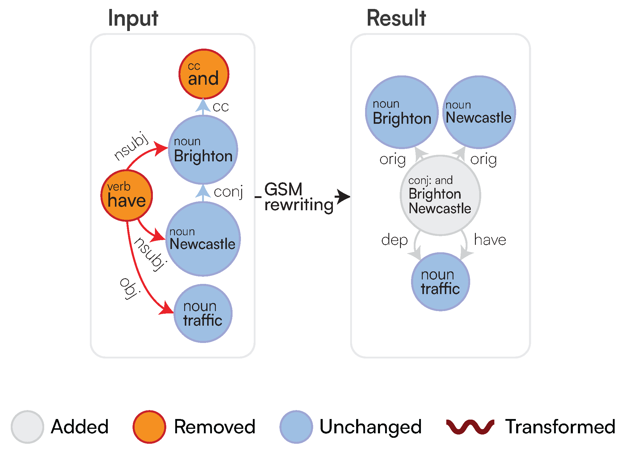
Figure 8.
Example graph after the GSM rewriting for the sentence “become able to answer more questions” with node IDs overlayed in the middle of each node. Each node represents a word in the sentence, and each edge represents a UD.
Figure 8.
Example graph after the GSM rewriting for the sentence “become able to answer more questions” with node IDs overlayed in the middle of each node. Each node represents a word in the sentence, and each edge represents a UD.
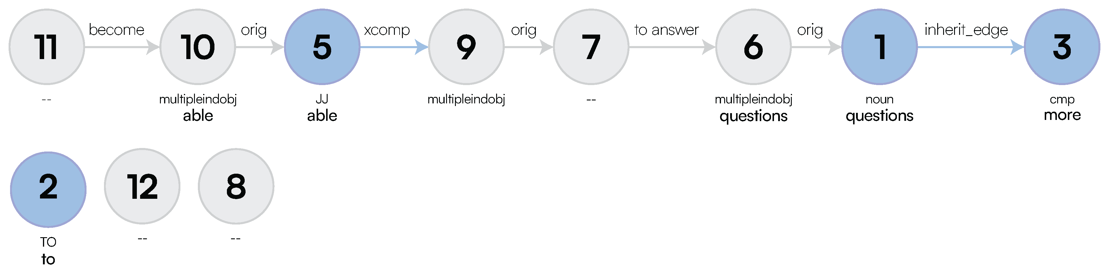
Figure 9.
Fragments of the Parmenides ontology encoding rules for capturing logical functions.
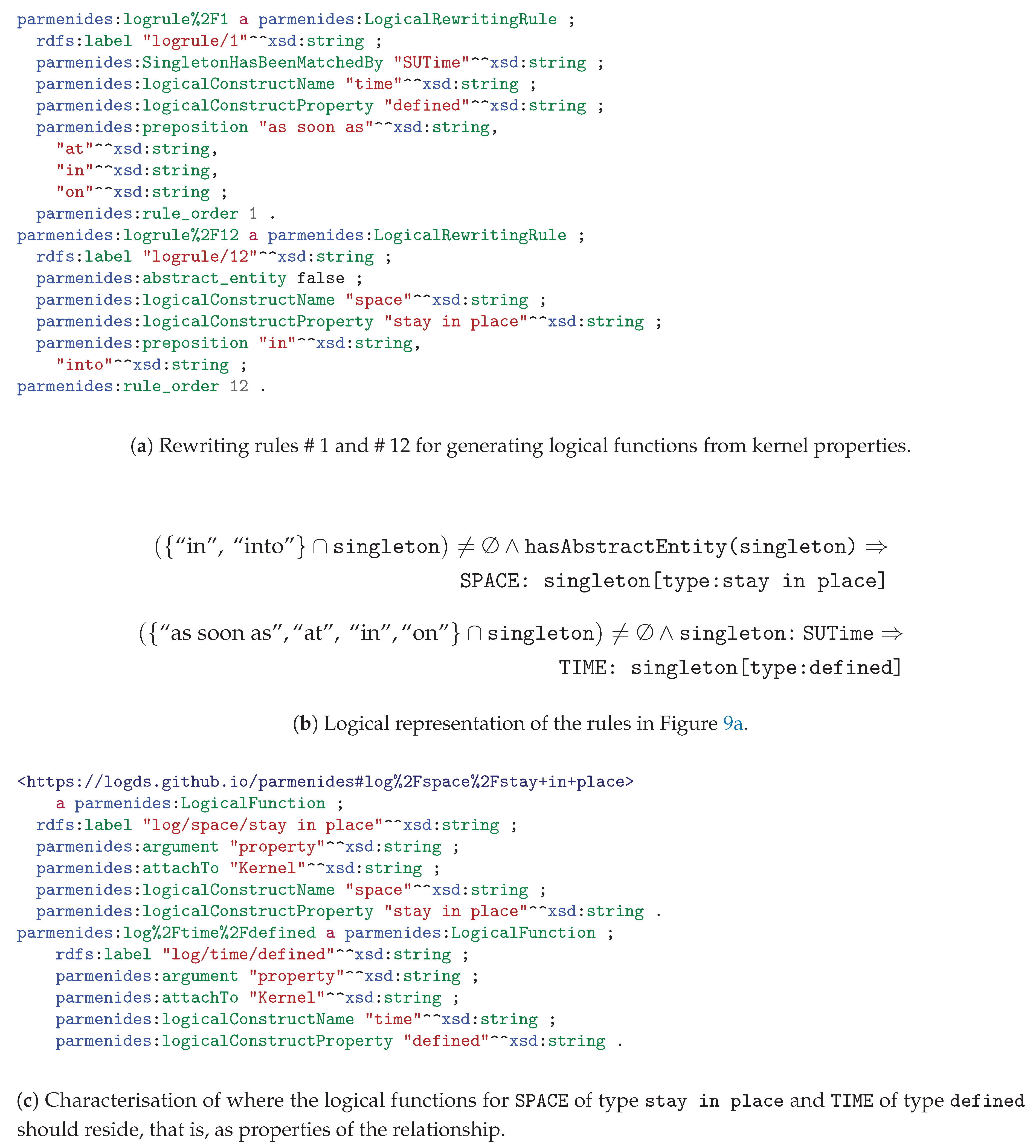
Figure 10.
Truth tables over admissible and compatible worlds for implying, indifferent, inconsistent, and equivalent atoms.
Figure 10.
Truth tables over admissible and compatible worlds for implying, indifferent, inconsistent, and equivalent atoms.
Figure 17.
The average (mean) number of vertices for varying sentence lengths (based on the number of nodes in each graph).
Figure 17.
The average (mean) number of vertices for varying sentence lengths (based on the number of nodes in each graph).
Figure 18.
Plot of scalability tests for the logical representation in log-norm scale.
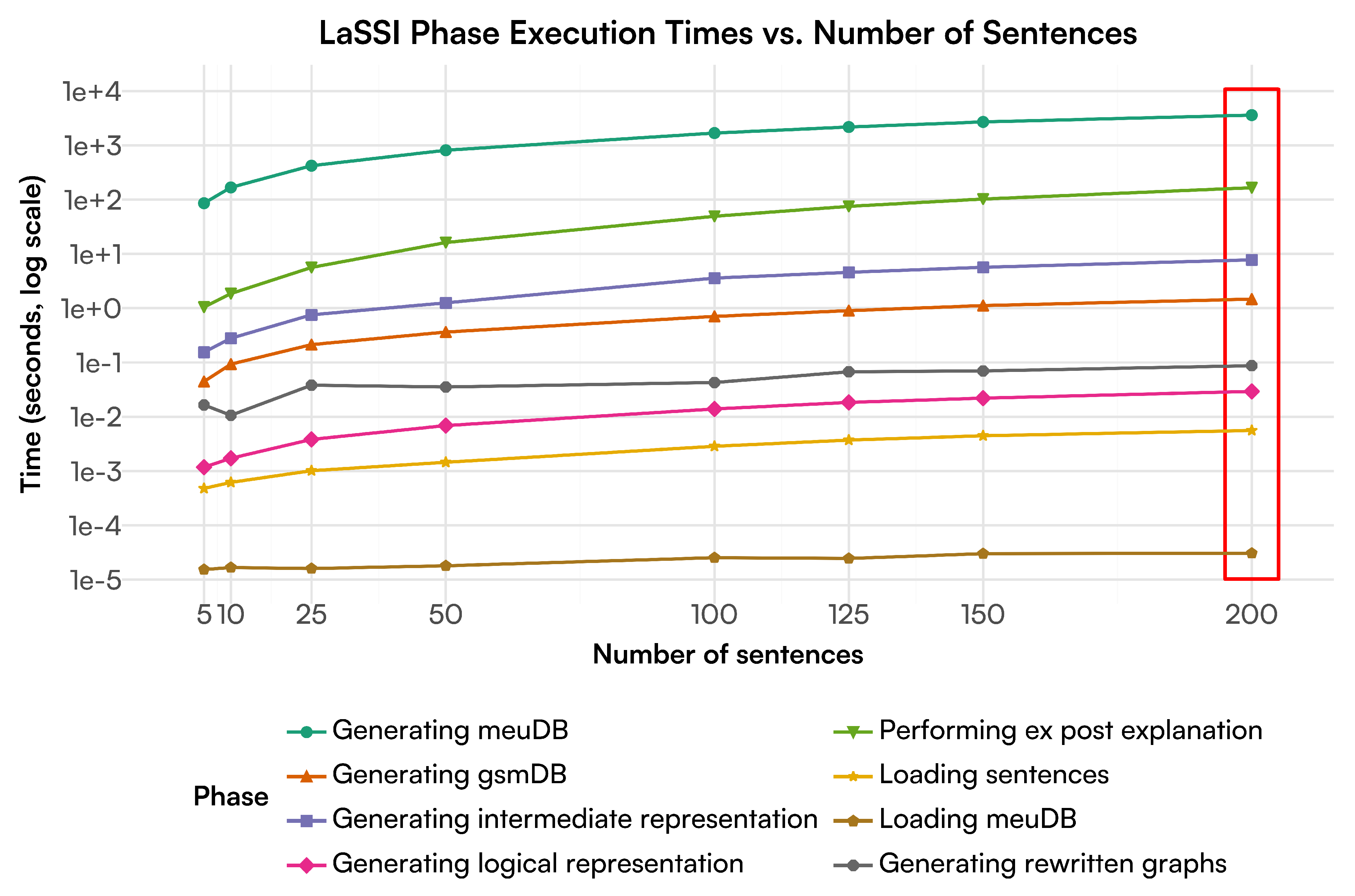
Figure 19.
Performance of each stage of the LaSSI pipeline for the logical representation (in log-norm scale) for sentences of different lengths (based on the number of nodes in each graph).
Figure 19.
Performance of each stage of the LaSSI pipeline for the logical representation (in log-norm scale) for sentences of different lengths (based on the number of nodes in each graph).
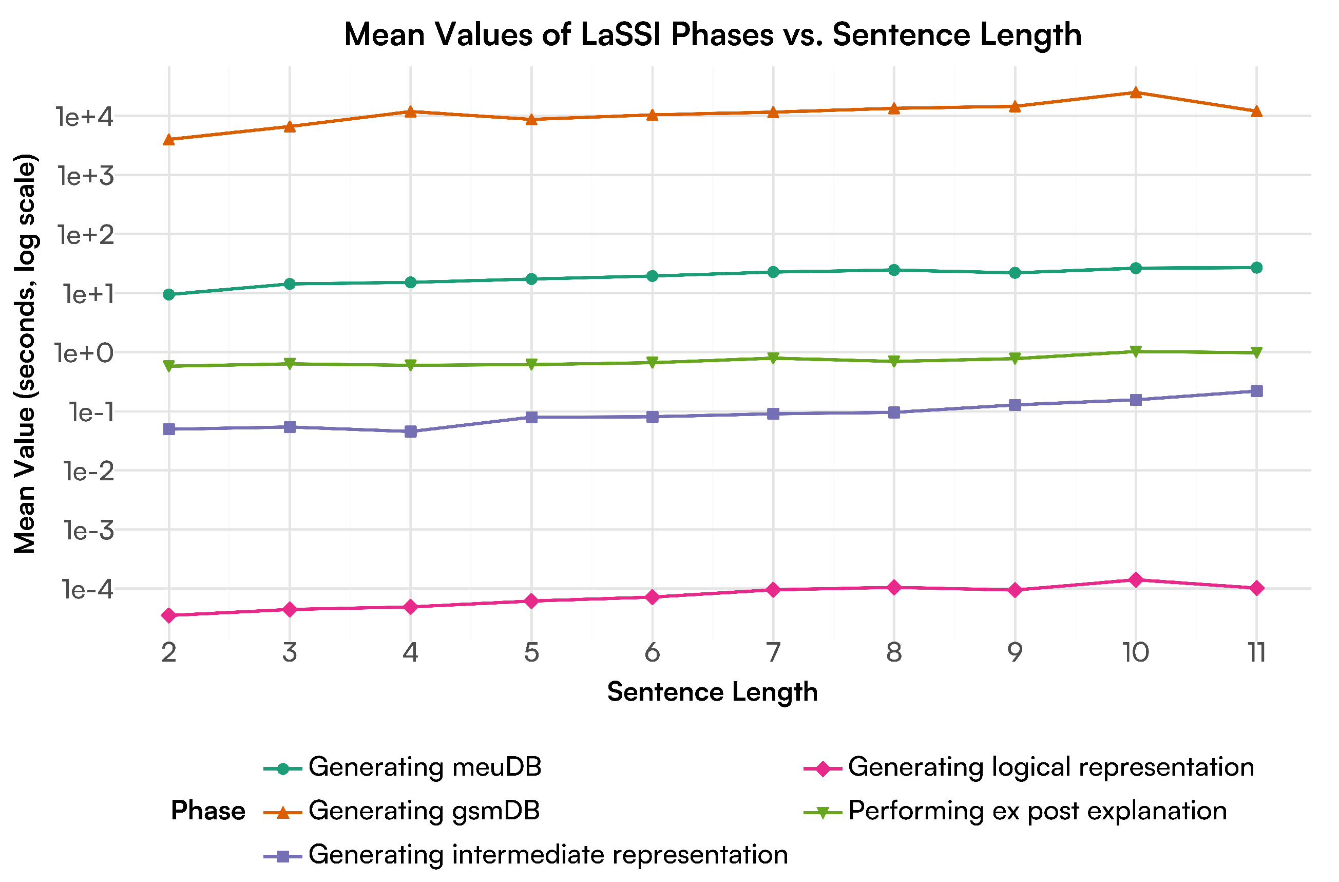
Figure 20.
Dendrogram clustering graphs for RQ №2(c) sentences, with comparisons when the ad hoc phase is disabled. Red and orange boxes represent the clusters for {0,1,9} and {6,7,8} respectively.
Figure 20.
Dendrogram clustering graphs for RQ №2(c) sentences, with comparisons when the ad hoc phase is disabled. Red and orange boxes represent the clusters for {0,1,9} and {6,7,8} respectively.
Figure 21.
LIME and SHAP explanations comparing “There is traffic but not in the Newcastle city centre” against itself.
Figure 21.
LIME and SHAP explanations comparing “There is traffic but not in the Newcastle city centre” against itself.
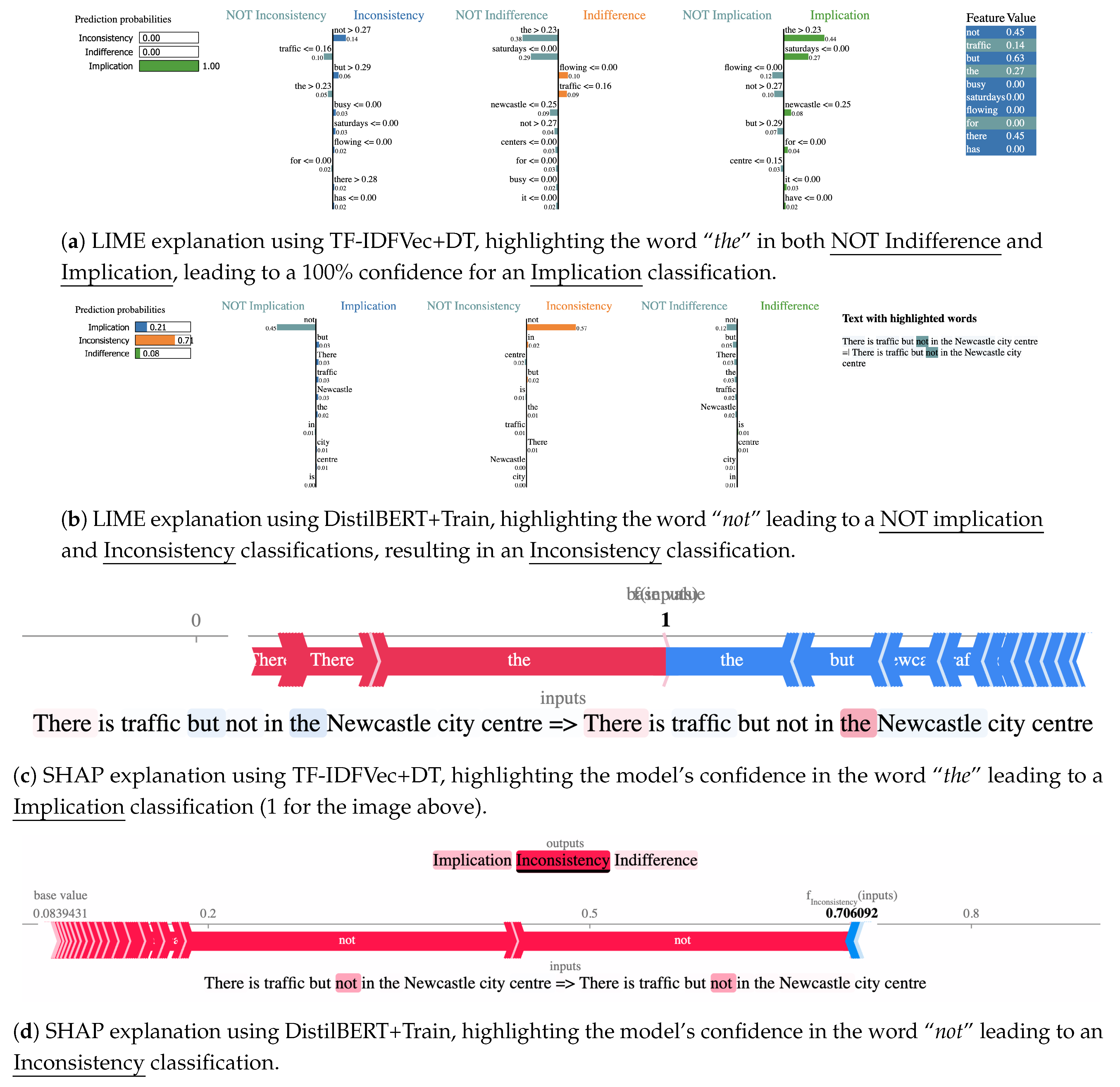

Table 1.
Some examples of logical functions considered in the current LaSSI pipeline beyond the simple subject–verb–direct object categorisation. These are then categorised and explained in our Parmenides ontology (Section 3.2.3), where these are not only defined by the POS tags and the associated prepositions but also by the type of verb and entity associated with them.
| Logical Function | (Sub)Type | Example (underlined) |
|---|---|---|
| Space | Stay in place | “I sit on a tree.” |
| Space | Motion to place | “I go to Bologna.” |
| Space | Motion from place | “I come from Italy.” |
| Space | Motion through place | “Going across the city center.” |
| Cause | – | “Newcastle is closed for congestion” |
| Time | Continuous | “The traffic lasted for hours” |
| Time | Defined | “On Saturdays, traffic is flowing” |
Table 2.
A comparative table between the competing pre-trained language model approaches and LaSSI.
| Sentence Transformers (Section 2.4.1) | Neural IR (Section 2.4.2) | Generative LLM (Section 2.4.3) | GEVAI (Section 2.1) | |||
|---|---|---|---|---|---|---|
| MPNet [46] | RoBERTa [47] | MiniLMv2 [48] | ColBERTv2 [49] | DeBERTaV2+AMR-LDA [10] | LaSSI (This Paper) | |
| Task | Document Similarity | Query Answering | Entailment Classification | Paraconsistent Reasoning | ||
| Sentence pre-processing | Word Tokenisation + Position Encoding | •AMR with Multi-Word Entity Recognition •AMR Rewriting |
•Dependency Parsing •Generalised Graph Grammars •Multi-Word Entity Recognition •Logic Function Rewriting |
|||
| Similarity/Relationship inference |
Permutated Language Modelling |
– | Annotated Training Dataset |
Factored by Tokenisation |
•Logical Prompts •Contrastive Learning |
•Knowledge Base-driven Similarity •TBox Reasoning |
| Learning Strategy | Static Masking | Dynamic Masking | Annotated Training Dataset |
•Autoregression •Sentence Distance Minimisation |
||
| Final Representation | One vector per sentence | Many vectors per sentence | Classification outcome | Extended First-Order Logic (FOL) | ||
| Pros | Deriving Semantic Similarity through Learning | Generalisation of document matching |
Deriving Logical Entailment through Learning | •Reasoning Traceability •Paraconsistent Reasoning •Non biased by documents |
||
| Cons | •Cannot express propositional calculus •Semantic similarity does not entail implication capturing |
•Inadequacy of AMR Representation •Reasoning limited by Logical Prompts •Biased by probabilistic reasoning |
Heavily Relies on Upper Ontology | |||
Table 3.
Truth table of values for sentences and .
| #W | ||||
|---|---|---|---|---|
| #1 | 0 | 0 | 0 | 0 |
| #2 | 0 | 1 | 0 | 1 |
| #3 | 1 | 0 | 0 | 1 |
| #4 | 1 | 1 | 1 | 1 |
Table 4.
Clustering scores for RQ №2(a) sentences, with the best value for each row highlighted in bold blue text and the worst values highlighted in red.
Table 4.
Clustering scores for RQ №2(a) sentences, with the best value for each row highlighted in bold blue text and the worst values highlighted in red.
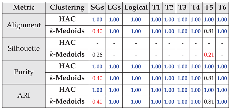 |
Table 5.
Classification scores for RQ №2(a) sentences; the best value for each row is highlighted in bold, blue text and the worst values are highlighted in red. The classes are distributed as follows: implication: 15; inconsistency: 16; indifference: 33.
Table 5.
Classification scores for RQ №2(a) sentences; the best value for each row is highlighted in bold, blue text and the worst values are highlighted in red. The classes are distributed as follows: implication: 15; inconsistency: 16; indifference: 33.
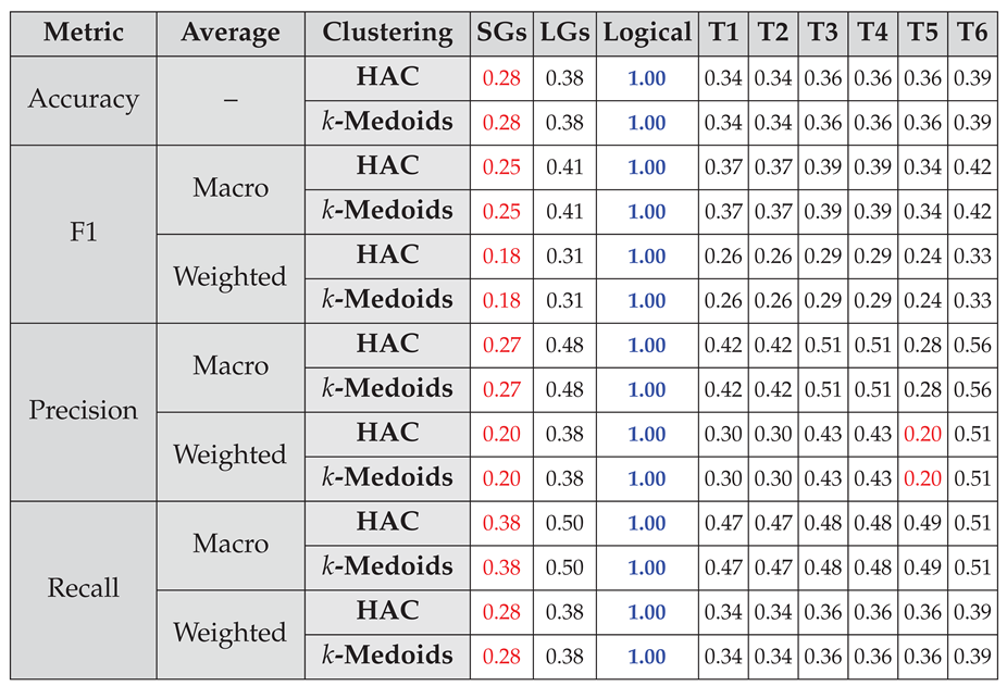 |
Table 6.
Clustering scores for RQ №2(b) sentences, with the best value for each row highlighted in bold, blue text and the worst values highlighted in red.
Table 6.
Clustering scores for RQ №2(b) sentences, with the best value for each row highlighted in bold, blue text and the worst values highlighted in red.
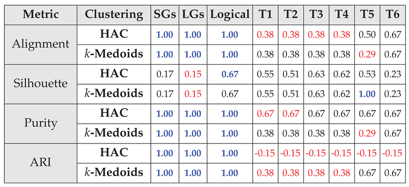 |
Table 7.
Classification scores for RQ №2(b) sentences, with the best value for each row highlighted in bold, blue text and the worst values highlighted in red. The classes are distributed as such: Implication: 10, Inconsistency: 8, Indifference: 18.
Table 7.
Classification scores for RQ №2(b) sentences, with the best value for each row highlighted in bold, blue text and the worst values highlighted in red. The classes are distributed as such: Implication: 10, Inconsistency: 8, Indifference: 18.
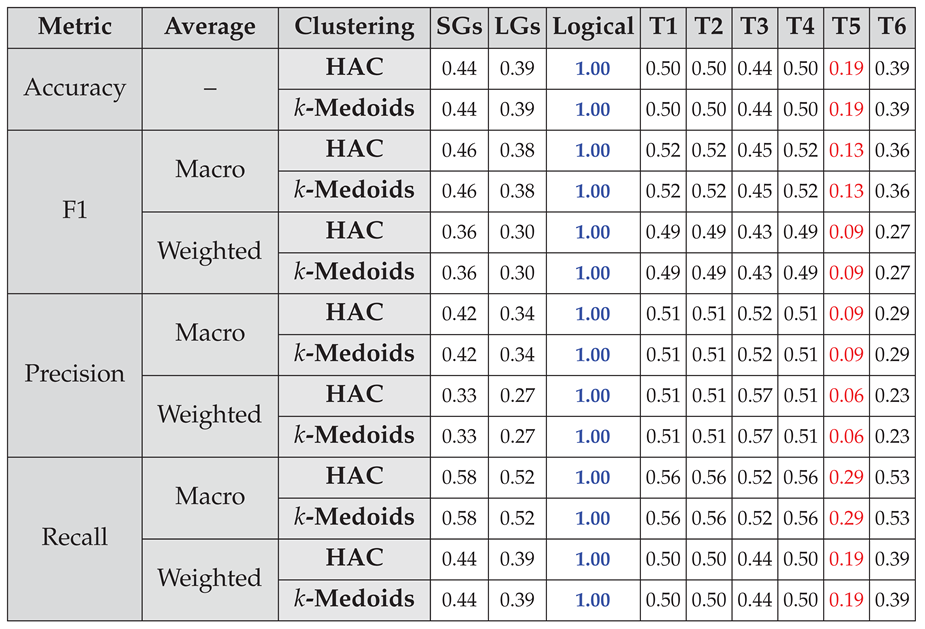 |
Table 8.
Clustering scores for RQ №2(c) sentences, with the best value for each row highlighted in bold, blue text and the worst values highlighted in red.
Table 8.
Clustering scores for RQ №2(c) sentences, with the best value for each row highlighted in bold, blue text and the worst values highlighted in red.
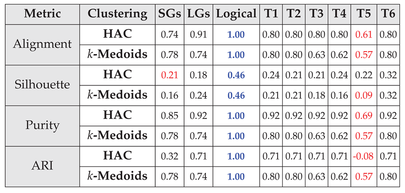 |
Table 9.
Classification scores for RQ №2(c) sentences, with the best value for each row highlighted in bold, blue text and the worst values highlighted in red. The classes are distributed as such: Implication: 32, Inconsistency: 27, Indifference: 110.
Table 9.
Classification scores for RQ №2(c) sentences, with the best value for each row highlighted in bold, blue text and the worst values highlighted in red. The classes are distributed as such: Implication: 32, Inconsistency: 27, Indifference: 110.
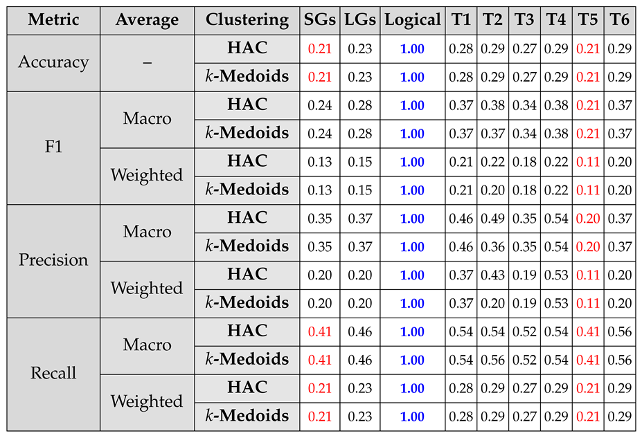 |
Table 10.
Classification scores for RQ №2(c) sentences, comparing transformation stages with a priori phase disabled in each case.
Table 10.
Classification scores for RQ №2(c) sentences, comparing transformation stages with a priori phase disabled in each case.
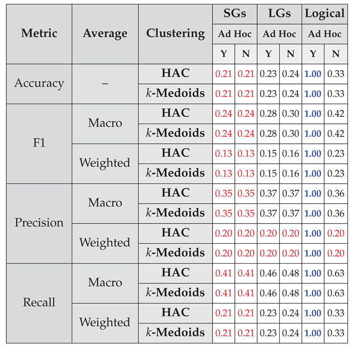 |
Table 11.
Performance degradation when training a preliminary model used by the explainer to correlate parts of text to the classification label.
Table 11.
Performance degradation when training a preliminary model used by the explainer to correlate parts of text to the classification label.
| Accuracy | F1 | Precision | Recall | ||||
|---|---|---|---|---|---|---|---|
| Macro | Weighted | Macro | Weigthed | Macro | Weighted | ||
| TF-IDFVec+DT | 0.95 | 0.93 | 0.94 | 0.95 | 0.94 | 0.92 | 0.94 |
| DistilBERT+Train | 0.76 | 0.51 | 0.69 | 0.45 | 0.64 | 0.61 | 0.76 |
Table 12.
Comparison table from the artefact evaluation. • = satisfies requirement; ◐ = partially satisfies requirement; ○ = does not satisfy requirement.
Table 12.
Comparison table from the artefact evaluation. • = satisfies requirement; ◐ = partially satisfies requirement; ○ = does not satisfy requirement.
| Explainer | Model | Req №1 | Req №2 | Req №3 | Req №3(a) |
|---|---|---|---|---|---|
| SHAP | TF-IDFVec+DT | ◐ | • | ◐ | ○ |
| DistilBERT+Train | ○ | • | ◐ | ○ | |
| LIME | TF-IDFVec+DT | ◐ | • | ◐ | ○ |
| DistilBERT+Train | ○ | • | ◐ | ○ | |
| LaSSI | • | ○ | • | • | |
Disclaimer/Publisher’s Note: The statements, opinions and data contained in all publications are solely those of the individual author(s) and contributor(s) and not of MDPI and/or the editor(s). MDPI and/or the editor(s) disclaim responsibility for any injury to people or property resulting from any ideas, methods, instructions or products referred to in the content. |
© 2025 by the authors. Licensee MDPI, Basel, Switzerland. This article is an open access article distributed under the terms and conditions of the Creative Commons Attribution (CC BY) license (http://creativecommons.org/licenses/by/4.0/).
Copyright: This open access article is published under a Creative Commons CC BY 4.0 license, which permit the free download, distribution, and reuse, provided that the author and preprint are cited in any reuse.


