
Submitted:
27 March 2025
Posted:
31 March 2025
You are already at the latest version
Abstract
Extreme temperature or heat wave events cause significant damage to socioeconomic activities and ecological systems. Over the past few decades, heatwave events in Pakistan have caused several health issues and increased mortality rates. This study analyzes the relationship and impact of temperature extremes of the northern Indian Ocean’s (IO) sea surface temperature (SST) and atmospheric temperature over land (ATL) for Pakistan. For this purpose, daily and monthly average atmospheric temperature over land (T2m) and SST were taken into account, and anomalies were calculated. It also analyzes the relationship between the Nino3.4 Index and northern IO’s SST and ATL. The seasonal (spring and summer) and monthly ( March-August) temperature extremes for Pakistan and the northern IO region have been analyzed over 5, 7, and 10-day stretch from 1979 to 2015. Results show that SST has a higher frequency of extreme temperature anomalies over different stretches of days than ATL. Temperature extreme anomalies were observed in northern IO’s SST during El Niño years. ATL was significantly prompted by SST when observed on a seasonal basis; however, an insignificant relationship was observed on a monthly basis. T2m and SST have shown a significant relationship with the Nino3.4 Index for sea and land. The results of this study would address the sustainable development goals (SDGs) focusing on hunger, good health and well-being, and climate action. It will further provide insight to policymakers for devising mitigation strategies against temperature extremes.
Keywords:
Thermal extremes
; Atmospheric temperature
; Sea surface temperature
; El Niño Southern Oscillation
; Indian Ocean
1. Introduction
World community in the 21st century is experiencing global warming due to rapidly increasing industrialization and human population density. Consequently, global warming and heat wave/thermal extreme events have received significant attention in this century due to their potential diminishing effect on socio-economic and ecological systems (Easterling et al. 2000; Fischer et al. 2012). Thermal extreme or heat waves cause significant damage to water resources, the energy sector, humans, crops, and animals (Burkey et al. 2015; Im et al. 2017). Thermal extreme is destructive to areas unfamiliar with such weather events, resulting in slow coping mechanisms (Cristo et al. 2007). Changes in the intensity, frequency, and duration of heatwave dipicts a strong relationship with anthropogenic warming (Dileepkumar et al 2021). With reference to the pre-industrial period (1860–1900), anthropogenic warming caused a rise of more than 1 °C in global mean temperature (GMT), which resulted in an increase in heatwave frequency and severity across the globe (Seneviratne et al. 2021). According to future projections by (Mani et al. 2018), the annual average temperatures will increase by 1.6 °C (2.9 °F) by 2050 in South Asia under the climate-sensitive scenario. As a consequence, heatwaves and heat stress will be more intense and frequent over South Asia .
Five or more consecutive days in which the daily maximum temperature surpasses the average maximum temperature by 5 ℃ or more is known as heat wave/thermal extreme event as described in the Britannica Encyclopedia. However, the definition to heat wave/thermal extremes may vary tremendously. For example, an increase of 5-6 ℃ or more above the normal temperature is required to be considered as thermal extreme by the India Meteorological Department whereas U.S. National Weather Service defines it as an “abnormally and uncomfortably hot and unusually humid weather” spanning over two or more days (Britannica Encyclopedia 2022). The geographic location of Pakistan is highly vulnerable to climate change, which lies in north of the Arabian Sea. The climate of Pakistan varies from arid to semi-arid, and temperature deviates from north to south (Ali et al. 2020; Khalid et al. 2018a). Studies on summer heat index have shown an intensification from 1961-2007 in different regions of Pakistan i.e., Punjab, southeast Baluchistan, northern region, and plains of Sindh, posing serious health issues (Chaudhary et al. 2009; Zahid and Rasul 2009). Zahid and Rasul (2012) calculated the frequency and intensity of heat waves and found an increasing trend in the Punjab, Sindh, and Baluchistan provinces. The extreme climatic events for different regions of Pakistan under different scenarios and periods have been investigated in several studies (c.f., Khan et al. 2019; Aslam et al. 2017, Zahid and Rasul 2012; Shelton and Dixon 2023). The 2015 heat wave event accounted for ~1200 deaths in Karachi, Pakistan. This heat wave caused soaring of temperatures throughout the country, including southern Punjab province (~40 ℃), Turbat (49 ℃), Larkana (49 ℃), and Sibbi (49 ℃) (Hanif 2017; Chaudhry et al. 2015). Pakistan’s agricultural productivity and economic efficiency have been negatively affected by heat waves; affecting the yield of rice, wheat and cereals (Arshad et al. 2018). Thermal extremes are related to general comfort, human health risk, and socioeconomic activities in different parts of the world e.g., Karachi, Shanghai, Paris, and Chicago etc. (Hanif 2017; Mazhar et al. 2015; Tan et al. 2007; Rey et al. 2009; Klinenberg 2002). Since Pakistan is an agricultural country and its population greatly relies on the income generated from agricultural practices (c.f., Ahmed et al., 2018; Ali et al., 2020), this type of study is vital to help policymakers ensure timely mitigation actions. Studying thermal extremes is important to meet some sustainable development goals, such as those related to climate action, resilience, hunger and poverty, good health, and well-being.
The IO on the globe is the only ocean bounded by tropical latitude (26 °N) (Josey et al. 1999). The stored energy of the ocean in this part enters into the atmosphere through the process of transpiration and evaporation while the remaining heat travel towards southern IO by Ekman currents during Jun-Sep (Levitus 1988). The IO heat content and SST are controlled by heat transport, subsequently affecting the inter-annual variability of the Asian monsoon (Godfrey et al. 1995; Garternicht and Schott 1997; Loschnigg and Webster 2000). Northern IO is limited to the tropical belt, which experiences semi-annual winds regulating the monsoon system over South Asia. Two modes of inter-annual variability, i.e., Indian Ocean Dipole (IOD) and El Niño Southern Oscillation (ENSO) have significant impacts on IO warming (Luo et al. 2010). ENSO events affect climate, weather conditions, terrestrial and marine ecosystems, and economies worldwide. The seasonality of ENSO and its impact on Indian summer monsoon and general weather systems have been reported by several researchers (c.f., Shukla and Huang 2016; Yang et al. 2015; Krishnaswamy et al. 2015; Cherchi and Navarra 2013; Wu et al. 2012; Achuthavarier et al. 2012; Luo et al. 2010). Similarly, the effects of ENSO on the weather systems of Bangladesh, Australia, India, Mozambique and Southwestern IO have been presented in several studies (c.f., Cash et al. 2010; Cai et al. 2011; Manhique et al. 2011; Ash and Matyas 2012).
A natural climate variability in the tropical IO i.e., Indian Ocean dipole (IOD), strongly affects the surrounding regions and the global climate (Qiu et al. 2014). Severe climatic events such as droughts and floods occur during the positive IOD event, which features a dipole mode of SST anomaly, coupling with equatorial easterly and oceanic adjustment (Yang et al. 2020). During the positive phase of IOD, droughts occur in Australia and Indonesia, whereas flooding in the coasts of western tropical IO The most destructive wildfires have occurred in Australia during positive IOD events (Boer et al. 2020; Nolan et al. 2020). IOD naturally develops as a result of Bjerknes feedback. The positive feedback may be triggered by anomalies such as zonal SST gradient, upwelling off Sumatra and the equatorial zonal wind and may cause the formation of IOD events (Zhang et al. 2018; Lu and Ren 2020). IOD is developed in boreal summer and attains maturity in fall, which depends on the initial conditions of the spring season. The warming in the tropical IO SST follows El Niño event and attains a peak in the boreal spring (Xie et al., 2016). The tropical IO SST has been modulating the low-level anticyclone over the western North Pacific and precipitation over central China (Cai et al. 2022). IO warming has been responsible for modulating the summer rainfall over east Asia (Chen et al., 2021). The extreme IO dipole has been regarded as a cause of IO warming (Zhou et al. 2021). The downwelling Kelvin waves during late spring to early summer reach the Sumatra-Java coast and cause the warming of SST over the southeastern tropical IO (Zhang and Du 2022). The warming of tropical IO has been studied in detail (c.f., Zhang and Du 2022; Xie et al. 2009); however, the impact of IO’s SST extremes over inland atmospheric temperatures still needs consideration to understand their relationship.
The general trends of precipitation and summer monsoon rainfall in Pakistan and in the Indian Subcontinent in connection to the variability in IO have been discussed in detail in the scientific literature (c.f., Iqbal and Athar 2018; Iqbal and Hassan 2018; Tamaddun et al. 2017; Hussain et al. 2017; Roxy et al. 2015; Khatri et al. 2015). However, a detailed study of the overall relationship and impact of temperature extremes and its variability in northern IO’s SST and its impact over Pakistan’s ATL; and impacts of ENSO on the SST of northern IO in connection to ATL in Pakistan have not been studied. Therefore, this study intends to focus on the aforementioned objectives in order to provide an understanding for bridging this research gap.
This study analyzes the ‘frequency of temperature extremes’ over northern IO’s SST and ATL and the connection of SST’s temperature extremes with ATL from March to August 1979-2015. Furthermore, the Nino3.4 Index is correlated with temperature (T2m) and SST over northern IO and Pakistan. ENSO and thermal extremes have been responsible for drought occurrences and flooding episodes in Pakistan (Khalid et al. 2018b; Zahid and Rasul 2012). The thermal extreme and its relation to ENSO are important to understand the occurrence of extreme weather events in Pakistan for a top-down policy approach to ensure best mitigation and adaptive actions.
2. Material and Methods
This study is conducted for the northern IO SST and Pakistan’s ATL, excluding the northern mountainous region (i.e., comprising of the mighty Himalayas and Karakoram ranges) (Figure 1). The datasets of Era5 at 0.25 degrees spatial resolution were obtained for daily T2m (i.e., atmospheric temperature over land and sea) and SST, monthly average atmospheric T2m and SST, and monthly average Nino3.4 Index were considered for calculating the correlations for the period of 1979-2015 over the study region.
The frequency of temperature extremes over Pakistan (i.e., ATL) and northern IO (i.e., SST) have been analyzed on monthly (i.e., March-August) and seasonal (i.e., spring (March-April-May (MAM)) and summer (June-July-August (JJA) basis for the period of 1979-2015. The linear regression analysis was performed to analyze the relationship between ATL and SST on a monthly and seasonal basis. Furthermore, the correlation of T2m and SST with the Nino3.4 Index was analyzed over land and sea.
The frequency of temperature extremes was calculated from 1979 to 2015 over the different stretches of days (i.e., 5, 7, and 10 days) in the study region. Daily ATL and SST were processed to calculate the threshold for temperature extremes; hence only the maximum observations were considered from the upper tercile. Maximum observations falling in the upper tercile were further distributed into three tiers for both seasons (spring and summer) separately, i.e., low, medium, and higher ranges. The higher range was considered the extreme temperature threshold for the respective season. For SST, the threshold intervals of temperature extremes are defined as [25.63℃, 27.18℃] for the spring season and [26.28℃, 27.53℃] for the summer season. Similarly, for ATL, the threshold intervals for temperature extremes are defined as [27.17 ℃, 34.27℃] for the spring season and [33.0℃, 36.0℃] for the summer season. These thresholds were tested for analyzing the frequency of temperature extremes. The anomalies for the frequency of temperature extreme events were calculated and plotted. If the temperature (i.e., ATL or SST) falls within the given threshold interval for consecutive 5, 7 or 10-day stretches for daily and seasonal observations during spring and summer, it is considered as extreme over the respective stretch of days (i.e., frequency). Therefore, temperature extremes over different stretches are analyzed in this study on a monthly and seasonal basis and their anomalous frequency has been plotted. The Mann-Kendall (MK) trend test was run to analyze the trend in seasonal temperature extreme events over the study region for 1979-2015. It is a non-parametric test used to analyze the significant trends in a time series (Mann 1945; Kendall 1975; Yue et al. 2002).
3. Results
3.1. Frequency of Monthly Temperature Extremes
The anomalies (of temperature extreme frequency) over 5, 7, and 10-day stretches for ATL and SST was analyzed on a monthly basis from March-August (1979-2015). No anomalies of SST and ATL occurred for 5, 7, and 10-day stretches in March (1979-2015). Figure 2a shows two peaks of temperature extreme anomalies for SST in 5-day stretch in April (1979-2015) (i.e., in the years 1998 and 2010). ATL shows several peaks of anomalies in the 5-day stretch; however, it remained less than SST in April throughout the study period. Figure 2b shows a similar trend (as in Figure 2a) of ATL and SST in April for 7-day stretch. Figure 2c shows several peaks of anomalies for SST and ATL in 10-day stretch in April (1979-2015) (i.e., in the years 1984 and 1999). Figure 2d,f shows sustaining anomalies of ATL and SST during May (1979-2015) in all 5, 7, and 10-day stretches. ATL remained less than SST; however, both parameters were observed with higher number of anomalies in May than April. Figure 3a shows around thirty peaks of anomalies for SST in 5-day stretch during June (1979-2015). Twenty peaks of anomalies for ATL in 5 and 7-day stretches were observed, and ten peaks in 10-day stretches for SST and ATL in June (1979-2015) were observed (Figure 3b,c). Figure 3d shows four peaks of anomalies for ATL in 5-day stretch in different years (i.e., 1986, 1994, 1997, and 2006) in July (1979-2015). Only one peak of an anomaly for SST was observed in 1983 for a 5-day stretch. Figure 3e shows there was only one peak of an anomaly for SST (i.e., in 1983) and ATL (i.e., in 2006) in June (1979-2015) for a 7-day stretch. Figure 3f shows two peaks of anomalies for ATL (i.e., in 1987 and 2006) and one peak for SST (i.e., in 1983) in July (1979-2015) for 10-day stretch. No anomalies were observed over different stretches in August (1979-2015).
3.2. Frequency of Seasonal Temperature Extremes
The anomalies for frequency of seasonal temperature extremes (i.e., spring and summer) of ATL and SST for 1979-2015 were calculated for 5, 7 and 10-day stretches. Figure 4a shows two peaks of anomalies for SST (i.e., in 1998 and 2010) in a 5-day stretch and four peaks for ATL (i.e., in 1998, 2000, 2007, and 2010) in 5-day stretch during the spring season (i.e., MAM (1979-2015)). Figure 4b,c shows two peaks of anomalies for SST (i.e., in 1998 and 2010) in 7-day stretch and two peaks in 10-day stretch; two peaks of anomalies for ATL (i.e., in 2001 and 2007) in 7-day stretch and two peaks in 10-day stretch during the spring season (i.e., MAM (1979-2015)). Figure 4d,e shows around seven peaks of anomalies for SST in the summer season (i.e., JJA (1979-2015)), whereas for ATL, it remained less than ten peaks within any year for both 5 and 7-day stretches. Figure 4f shows ten peaks of anomalies for SST in 10-day stretch, whereas ATL remained quite less (i.e., 5 peaks) in 10-day stretch during the summer season (i.e., JJA (1979-2015)).
The narrow range of SST whereas a wide range of ATL was observed for the frequency of temperature extreme anomalies during the spring season (1979-2015), the range overlapped with each other (Figure 5). During the summer season the range of both parameters is narrow and does not overlap with each other. The range of frequency of temperature extreme anomalies for SST and ATL is higher during the summer season compared to the spring season. Figure 6 shows R² = 0.798 for the spring season, indicating a significant positive relationship between ATL and SST. Figure 6b shows R² = 0.524 and a positive relationship between ATL and SST in the summer season. Figures S1–S4 (Supplementary Material) & Table 1 shows a monthly and seasonal linear regression analysis of ATL and SST for April-July during 1979-2015. The negative relationships were found for 5, 7 and 10-day stretches of thermal extremes between ATL and SST on a monthly basis.
The Ʈ indicates the magnitude of trends, and Sen’s slope validates the results obtained from the p-value in the MK trend test (Table 2). The significant trend has been found in SST temperature extreme events in both seasons. No significant trend was found in ATL in the spring season, whereas a significant trend was observed in ATL in the summer season.
Figure S5a,b (Supplementary Material) shows a significantly increasing trend of SST and an insignificant trend for ATL observed in the spring season. Figure S5c,d shows a significantly increasing trend of SST and a significantly decreasing trend of ATL in the summer season. Figure S6 (Supplementary Material) shows the spatial distribution of SST over the study region in the spring and summer seasons. The springtime SST is warmer as compared to the summertime SST.
3.3. Correlation of T2m & SST with Nino3.4 Index
Figure 7 shows the spatial distribution of correlation between the monthly NINO3.4 index and T2m over land and ocean. There is a negative correlation of the Nino3.4 Index with T2m in March and April over large parts of land and IO; however, it shows a positive relationship in May on a large part of IO The strong positive correlation is shown in June, July, and August over land and IO Figure 8a,b shows the spatial distribution of T2m (shaded; ℃) superimposed on 850 hPa wind (vector; ms-1) on a seasonal basis. Strong winds from warm IO enter the land during the summer, strengthening the ATL. A strong positive correlation between the Nino3.4 Index and T2m has been observed over the entire study region (land and ocean) in the summer, whereas a weak to no correlation is observed in the spring (i.e., weak correlation over the ocean and no correlation over land). Figure 9a,b shows the spatial distribution of SST (shaded; ℃) on a seasonal basis. A statistically significant correlation between the NINO3.4 index and SST has been observed at a 90% confidence interval in both seasons. Figure 10a–f shows the spatial distribution of correlation between the monthly NINO3.4 index and SST.There is a strong positive relationship of both parameters in all studied months.
4. Discussion
We analyzed the frequency of temperature extreme events of ATL over Pakistan (i.e., land) and SST of northern tropical IO over different stretches of days (5, 7 and 10-day stretches) and calculated anomalies were plotted. 2m temperature and SST were correlated with the Nino3.4 Index from 1979 to 2015 on a monthly (i.e., March-August) and seasonal basis (i.e., spring and summer) over land and IO to see if there is any effect of Nino3.4 Index over the warming of the study region.
The temperature extremes did not show any significant inclusion in the pre-determined threshold interval for March and August (1979-2015) for 5, 7 and 10-day stretches for ATL and SST. Since March and August are the months of seasonal variations and weather transition, the temperature over land and sea changes abruptly. In March, the weather transition from winter to spring occurs, and in August, the weather transition from summer to autumn begins over Pakistan and northern IO ATL and SST do not remain consistent over the study region at this time (i.e., March and August); hence, the sustaining thermal extremes for 5, 7 or 10-day stretches did not show occurrence over the study region. However, several peaks in the frequency of temperature extremes have been observed in anomalies for different day stretches from April to July (1979-2015). More anomalies have been observed for SST in April in 1998 and 2010 and ATL in 2007. In May, anomalies for SST were observed in the years 1979, 1982, 1988, 1994, 1997, 2003, 2006, 2012, and 2015 and for ATL in the years 1984, 1987, 1990, 1998, 1999, 2000, 2001, 2010, and 2015. In June, anomalies for SST have increased as compared to ATL. SST anomaly peaks have been observed in 1982, 1983, 1987, 1988, 1991, 1995, 1997, 2003, 2009, 2010 and 2015. However, ATL anomaly peaks are observed only in 1979, 1981, and 1994. In July, the frequency of temperature extreme for SST and ATL showed a quite different pattern as compared to previous months. The temperature extreme events over 5, 7 and 10-day stretches for both parameters (i.e., SST and ATL) started to disappear in July. For SST in July, the peak was observed in the year 1983 and for ATL the peak was observed in the years 1995, 1997, and 2006. Overall, anomalies in 5- and 7-day stretches have been observed more frequently than 10-day stretches in April, May, June, and July. The 10-day stretch has a higher number of anomaly peaks in June. Anomalies started to peak in April, sustained through May and June, and disappeared in July for T2m. The results of temperature variations (T2m) over Pakistan shown in this study are consistent with other studies (c.f., Rashid et al., 2022); however, in this study, we have discussed it in terms of anomalies. MK trend test shows an increased frequency of temperature extremes over SST than ATL in spring, whereas a significant prevalence of temperature extreme events occurs in summer over both SST and ATL.
El Niño events have been observed during 1982-1983, 1997-1998, and 2014-2016. During El Niño years, the thermal extremes of SST prevail over northern tropical IO in May and June. The years of thermal extremes during April-July (1979-2015) have been italicized and underlined in the above paragraph, which was observed during El Niño years. During El Niño years, Pakistan faces a rainfall deficit during the summer monsoon season (Khalid et al. 2018b); hence, the arid and semi-arid regions experience thermal extremes without cooling effect. Therefore, El Niño has contributed to the differential heating in northern IO SST in the study region.
More anomalies have been observed for SST compared to ATL for 5, 7, and 10-day stretches in both spring and summer seasons. The results of our study are in accordance with the study of Yoo et al. (2006), the SST seasonal fluctuation over the northern IO and the equator reaches the maximum in the spring season (i.e., MAM) and is sustained until the start of the summer season (i.e., JJA). There is more fluctuation and a wide range of temperature extreme anomalies for ATL, whereas there is a narrow range of temperature extreme anomalies for SST during the spring season. There is a narrow range of temperature extreme anomalies for both SST and ATL in the summer season.
ATL has been significantly prompted by SST fluctuations (i.e., 80% variability of ATL by SST) in the seasonal and monthly effect; however, monthly analysis shows less variability of the response data around its mean for March and August only. The ATL has been significantly prompted by SST fluctuations on a monthly basis for 5 and 7-day stretches whereas insignificantly prompted by SST for 10 days stretch. It shows only 0-10% variability of ATL explained by SST for the 10 days stretch on a monthly basis. For thermal extremes of SST, an increasing trend is observed in summer and spring, whereas for ATL, a slightly increasing trend in spring and a decreasing trend in summer are observed. Similar increasing trends of differential heating over IO have been described in several studies (c.f., Stocker et al. 2013; Han et al. 2010; Pervez and Henebry 2016).
In the tropical and northern IO, May exhibits the highest value, whereas Jun-Aug exhibits the second highest value of SST. The physical mechanism of warming of temperatures over land due to SST warming in the northern IO region is led by the air-sea interaction process and its effect on the monsoon system. As the SST in the north IO region (i.e., the Bay of Bengal and the Arabian Sea) rises, it generates a temperature gradient between the ocean and the land, which is more prominent during pre-monsoon and monsoon seasons (i.e., June, July, August, September). Warmer SST causes warming of the overlying atmosphere. Less dense and rising warmer air in the overlying atmosphere develops a low-pressure system over the parts of warmer IO, which creates a pressure gradient between the ocean (low pressure) and the land (higher pressure).
Due to this pressure gradient, the monsoon winds are generated, bringing in the moisture-laden air masses from over the ocean to the inland. A significant amount of moisture is carried inland the Indian subcontinent due to these moist air masses. As the moist monsoon air touches the higher terrain of the Western Ghats in India, it rises, cools and condenses to form clouds and cause rainfall. By the process of condensation, as the latent heat is released, the adiabatic warming further warms the surrounding atmosphere creating a warming effect for increasing temperature over the land. The surface temperatures are cooled temporarily due to monsoon rainfall and associated latent heat absorption and evaporation processes. The adiabatic warming and accumulated moisture assist in gradually raising the temperature of the land after subsiding of monsoon rains. This interaction of land temperatures and IO warming is a significant process of seasonal fluctuations in the study region.
The northern IO’s cooling is caused by monsoon activity from July to Sep (Yoo et al. 2006). In general, insignificant variations occur in SST over the IO from Jun-Sep, with the highest SST occurrence in Jun-Aug over tropical and equatorial IO. SST has changed over northern tropical IO, whereas SST increases over western IO due to weak monsoon (Yoo et al. 2006). The tropical IO has regional differences in SST patterns due to different wind directions i.e., from northeast in winter and southwest in summer. The winds from the southwest direction are generated by differences of atmospheric pressure from Asia’s warmer temperatures and southern IO’s cold temperatures during the summer and spring, respectively (Hastenrath and Lamb 1979). The higher thermal variability occurs in connection to SST in the southern to central region of Pakistan as compared to the northern region. The large deserts of India and Pakistan also regulates the thermal activity in the southern to central region, fluctuate temperatures well, and participate in intensified events (Rasul et al. 2012).
A positive relationship has been observed between the Nino3.4 Index and T2m (1979-2015) on a monthly and seasonal basis. The strengthened relationship has been observed over sea than land in March-May; however, a strong positive correlation is obtained for the entire study region in June-August. A strong positive relationship has been observed between the Nino3.4 Index and SST (1975-2015) on a monthly and seasonal basis. Hanley et al. (2003) described several regions for ENSO but highlighted the Nino3.4 region having a mixed and deep layer, which prevents/suppresses the thermal extreme from occurring, hence sustaining the physical characteristics in the region.
The physical mechanism of ENSO and IO warming is described by the weakening of the Walker Circulation due to El Niño event that affects the Indian Ocean Basin-Wide Mode (IOBW) and IOD. These climatic modes in IO affect the SST and weather patterns in IO region. The positive phase of IOD and the weakened Walker Circulation during El Niño phase bring drier and warmer conditions to the northern IO region, resulting in higher SSTs. This warming of northern IO may affect the normal patterns of pre-monsoon and monsoon seasons and may cause changes in temperature and rainfall patterns in adjacent inland regions. The northern IO warming also influences the local and regional climatic patterns, developing feedback mechanisms that may extend or strengthen the effects of El Niño on the region. These warming effects of El Niño have significant socioeconomic impacts on the adjacent regions' ecosystems, agriculture, and water resources.
El Niño events are responsible for modulating the temperature extremes over the subcontinent during the spring season (Joshi et al., 2020). The spring (MAM) asymmetric mode is a robust climate variability in the tropical IO, which is developed following the positive wind-evaporation-SST (WES) feedback (Wu et al., 2008). The spring asymmetric mode creates strong disturbances along the equator and modulates the following IOD phase development from late spring or early summer (Zhang and Du, 2022). During the positive IOD events, the downwelling Rossby wave transport may trigger the SST warming and the asymmetric mode in late spring to early summer (April-June). The easterly wind anomalies in the eastern and central equatorial ocean favor SST cooling. In the following months, the equatorial easterly wind anomalies trigger the positive Bjerkness feedback and induce the positive IOD in the following fall (i.e., September) (Zhang and Du, 2022). In the present study, the IO SSTs are affected by the El Niño events in the spring and summer during the years of climate variability, and the IO SSTs modulate thermal extremes in ATL in April-July during the studied years, which is apparent in the light of the analysis for IO warming in the respective seasons.
5. Conclusions
This study intends to analyze the frequency of monthly and seasonal temperature extremes (SST and ATL) over Pakistan and Northern IO over the period of 1979-2015. The temperature extreme thresholds were calculated for high ranges of maximum observations (upper tercile) of maximum temperature over the study region. The temperature extremes were calculated on a monthly and seasonal basis for 5, 7, and 10-day stretches. The consecutive prevalence of temperature (i.e., SST and ATL) over a specific number of days falling within the respective threshold interval of temperature extremes determined the frequency of events within the defined stretch of days. The anomalies in T2m and SST were analyzed to see the variations in temperature extremes and whether the variations in SST are affecting the variations in ATL over Pakistan. Furthermore, the T2m and SST were correlated with the Nino3.4 index. Results show that SST has higher frequency of extreme temperature events over the analyzed stretch of days (on a monthly basis) than ATL. For summer season, April-July (1979-2015) showed several peaks of anomalies for 5, 7, and 10-day stretch. ATL significantly impacts SST in seasonal effects (in both summer and spring seasons). A significant positive relationship has been observed between the Nino3.4 Index and T2m (1979-2015) on a monthly and seasonal basis. SST shows higher variations than ATL when correlated with the Nino3.4 Index; however, a statistically significant relationship was observed during the spring season for T2m over IO Similarly, SST shows a significant positive relationship with the Nino3.4 Index on a seasonal and monthly basis and shows a higher percentage of dependency on the Nino3.4 Index.
Communities and governments can better anticipate and respond to climate change by understanding temperature extremes and their patterns. Understanding temperature extremes and its patterns is essential for achieving SDGs such as improved climate resilience under SDG13-Climate Action, which focuses on combating climate change and its impacts. Such research improves our capacity to anticipate and react to extreme occurrences like heatwaves, cold snaps, and severe storms, which helps develop more accurate climate models and early warning systems. Such studies also help in better understanding, anticipating and managing the risks related to crops and food production, hence assisting in SDG2-Zero Hunger. The results of this study shall assist communities in the mitigation of the impacts of extreme temperatures and, adaptation of safe agricultural practices, and effectively dealing with temperature-related challenges. Studies on temperature extremes are crucial in urban planning and infrastructure development (SDG11-Sustainable Cities and Communities) and in mitigating the impacts of heat waves for health risks (SDG3-Good Health and Well-being).
Supplementary Materials
The following supporting information can be downloaded at the website of this paper posted on Preprints.org.
Author Contributions
B.K. & S.M.A & A.K. designed the research. S.S. & A.I. performed the analysis. B.K. & A.I. interpreted the results. B.K. prepared the manuscript. F.I. & A.H. reviewed the manuscript for improvements.
Acknowledgments
Authors thank to Dr. Azmat Hayat Khan, Chief Meteorologist, Pakistan Meteorological Department for his sincere guidance and support in carrying out this study. Special acknowledgement has been expressed to China-Pakistan Joint Research Center on Earth Sciences, CAS-HEC, for supporting the execution and implementation of this study.
Conflicts of Interest
Authors declare no competing interest.
References
- Ali et al., 2020 S. Ali, B. Khalid, R.S. Kiani, et al. Spatio-Temporal Variability of Summer Monsoon Onset over Pakistan. [CrossRef]
- Asia-Pacific J. Atmos. Sci., 56 (2020), pp. 147–172.
- Arshad et al., 2018 M. Arshad, T.S.A. Babu, S. Aravindakshan, et al. Climatic variability and thermal stress in Pakistan’s rice and wheat systems: a stochastic frontier and quantile regression analysis of economic efficiency Ecological Indicators., 89 (2018), pp. 496-506. [CrossRef]
- Aslam et al., 2017 A. Aslam, S. Ahmad, I. Ahmad, et al. Vulnerability and impact assessment of extreme climatic event: A case study of southern Punjab, Pakistan Sci. Total Environ., 580 (2017), pp. 468-481. [CrossRef]
- Achuthavarier et al., 2012 D. Achuthavarier, V. Krishnamurthy, B.P. Kirtman, et al. Role of the Indian Ocean in the ENSO–Indian summer monsoon teleconnection in the NCEP Climate Forecast System J. Clim., 25 (2012), pp. 2490–2508. [CrossRef]
- Ash and Matyas, 2012 K.D. Ash, C.J. Matyas The influences of ENSO and the subtropical Indian Ocean Dipole on tropical cyclone trajectories in the southwestern Indian Ocean Int. J. Clim., 32 (2012), pp. 41-56. [CrossRef]
- Ahmed et al., 2018 Ahmed, K., Shahid, S. and Nawaz, N Impacts of climate variability and change on seasonal drought characteristics of Pakistan. Atmospheric Research, 214, 364–37. [CrossRef]
- Burke at al., 2015 Burke, M., Hsiang, S.M. and Miguel, EGlobal non-linear effect of temperature on economic productionNature, 527, 235–239.
- Britannica Encyclopedia, 2022 <https://www.britannica.com/science/heat-wave-meteorology> Accessed on 8 August 202.
- Boer et al., 2020 Boer, M. M., V. Resco de Dios, and R. A. Bradstock.
- Unprecedented burn area of Australian mega forest fires .
- Nat. Climate Change, 10, 171–172.
- Cai et al., 2020 Cai, Y., Chen, Z. & Du, YThe role of Indian Ocean warming on extreme rainfall in central China during early summer 2020: without significant El Niño influence Clim Dyn 59, 951–960.
- Chen et al., 2021 Chen Z, Li Z, Du Y, Wen Z, Wu R, Xie SP.Trans-basin influence of southwest tropical Indian Ocean warming during early boreal summer. J Clim 34(24):9679–9691. [CrossRef]
- Chaudhry et al., 2015 Z. Chaudhry, G. Rasool, A. Kamal, et al. Task Force/ Fact Finding Mission by GOP on Causes of Severe Heat Wave in KarachiTechnical Report. (2015).
- Cherchi and Navarra, 2013 A. Cherchi, A. Navarra.Influence of ENSO and of the Indian Ocean Dipole on the Indian summer monsoon variability. Clim. Dyn., 41 (2013), pp. 81–103. [CrossRef]
- Cai et al., 2011 W. Cai, P. van Rensch, T. Cowan, et al. Teleconnection pathways of ENSO and the IOD and the mechanisms for impacts on Australian rainfall. J. Clim., 24 (2011), pp. 3910–3923. [CrossRef]
- Cash et al., 2010 B.A. Cash, X. Rodó, J.L. Kinter III, et al.
- Disentangling the impact of ENSO and Indian Ocean variability on the regional climate of Bangladesh: Implications for cholera risk.J. Clim., 23 (2010), pp. 2817–2831.
- Chaudhary et al., 2009 Q.Z. Chaudhary, A. Mahmood, G. Rasul, et al. Climate change indicators of Pakistan. Technical Report No. PMD-22 (2009), pp. 1–43.
- Cristo et al., 2007 R.D. Cristo, A. Mazzarella, R. Viola. An analysis of heat index over Naples (Southern Italy) in the context of European heat wave of 2003. Nat. Haz., 40 (2007), pp. 373–379. [CrossRef]
- Easterling et al., 2000 D. Easterling, G. Meehl, C. Parmesan, et al. Climate extremes: observations, modeling, and impacts. [CrossRef]
- Sci., 289 (2000), pp. 2068–2074.
- Fischer et al., 2012 T. Fischer, M. Gemmer, L. Liu, L. et al. Change-points in climate extremes in the Zhujiang River Basin, South China, 1961–2007.Clim. Chang., 110 (2012), pp. 783–799. [CrossRef]
- Garternicht and Schott, 1997 U. Garternicht, F. Schott.Heat fluxes of the Indian Ocean from a global eddy-resolving model. [CrossRef]
- J. Geophy. Res., 102 (1997), pp. 147–159.
- Godfrey, 1995 Godfrey, J.S., 1995. The role of the Indian Ocean in the global climate system: Recommendations regarding the global ocean observing system. Ocean Observing System Development Panel Rep. 6. Texas A&M University, College Station, TX, pp. 89.
- Hanif, 2017 Hanif, U Socioeconomic impacts of heat wave in Sindh. Pak. J. Met., 13 (2017), pp. 87–96.
- Hussain et al., 2017 M.S. Hussain, S. Kim, S. Lee. On the relationship between Indian Ocean Dipole events and the precipitation of Pakistan Theor. App. Clim., 130 (2017), pp. 673–685. [CrossRef]
- Han et al., 2010 W. Han, G.A. Meehl, B. Rajagopalan, et al. Patterns of Indian Ocean sea-level change in a warming climate. [CrossRef]
- Nat. Geo., 3 (2010), pp. 546–550.
- Hanley et al., 2003 D.E. Hanley, M.A. Bourassa, J.J. O’Brien, et al. Quantitative evaluation of ENSO indices.J. Clim., 16 (2003), pp. 1249–1258.
- Hastenrath and Lamb, 1979 Hastenrath, S., Lamb, P.J., 1979. Climate atlas of the Indian Ocean. Surface climate and atmospheric circulation. University of Wisconsin Press, Madison., Vol. 1.
- Im et al., 2017 Im, E.S., Pal, J.S. and Eltahir, E.A.B. Deadly heat waves projected in the densely populated agricultural regions of South Asia.Science Advances, 3(8), 1–8. [CrossRef]
- Iqbal and Athar 2018 M.F. Iqbal, H. Athar Variability, Trends, and Teleconnections of Observed Precipitation over Pakistan.
- Theor. App. Clim., 134 (2018), pp. 613-632.
- Iqbal and Hassan, 2018 A. Iqbal, S.A. Hassan ENSO and IOD analysis on the occurrence of floods in Pakistan.Nat. Haz., 91 (2018), pp. 879–890. [CrossRef]
- Joshi et al., 2020 Joshi, M.K., Rai, A., Kulkarni, A. and Kucharski.Assessing changes in characteristics of hot extremes over India in a warming environment and their driving mechanisms.Scientific Reports, 10(1), 1–14. [CrossRef]
- Josey et al., 1999 A. Josey, E. Kent, P. Taylor New insights into the ocean heat budget closure problem from analysis of the SOC air–sea flux climatology. J. Clim., 12 (1999), pp. 2856–2880.
- Khan et al., 2019 N. Khan, S. Shahid, T. Ismail, et al. Trends in heat wave related indices in Pakistan. Stoch. Environ. Res.risk Asses., 33 (2019), pp. 287–302. [CrossRef]
- Khalid et al., 2018a B. Khalid, C. Bueh, S. Javeed, et al. The application of a single-model ensemble system to the seasonal prediction of winter temperatures for Islamabad and Lahore using coupled general circulation models Weather., 73 (2018a), pp. 159–164.
- Khalid et al., 2018b B. Khalid, B. Cholaw, D.S. Alvim, et al. Riverine flood assessment in Jhang district in connection with ENSO and summer monsoon rainfall over Upper Indus Basin for 2010. Nat. Haz., 92 (2018b), pp. 971–993.
- Khalid et al., 2015 B. Khalid, A. Ghaffar Dengue transmission based on urban environmental gradients in different cities of Pakistan. Int. J. Biomet., 59 (2015), pp. 267–283. [CrossRef]
- Khatri et al., 2015 Khatri, W.D., Xiefei, Z., Ling, Z., 2015. Interannual and Interdecadal Variations in Tropical Cyclone Activity over the Arabian Sea and the Impacts over Pakistan. In: Ray, K., Mohapatra, M., Bandyopadhyay, B. and Rathore, L. (eds) High-Impact Weather Events over the SAARC Region. Springer, Cham.
- Krishnaswamy et al., 2015 J. Krishnaswamy, S. Vaidyanathan, B. Rajagopalan, et al. Non-stationary and non-linear influence of ENSO and Indian Ocean Dipole on the variability of Indian monsoon rainfall and extreme rain events. Clim. Dyn., 45 (2015), pp. 175–184. [CrossRef]
- Klinenberg, 2002 Klinenberg, E., 2002. Heat Wave: A Social Autopsy of Disaster in Chicago. Chicago, IL: University of Chicago Press.
- Kendall, 1975 Kendall, M.G., 1975. Rank Correlation Methods, second ed. New York.
- Luo et al., 2010 J. Luo, R. Zhang, S.K. Behera, et al. Interaction between El Niño and Extreme Indian Ocean Dipole J. Clim., 23 (2010), pp.726–742. [CrossRef]
- Loschnigg and Webster, 2000 J. Loschnigg, P.J. Webster. A coupled ocean-atmosphere system of SST regulation for the Indian Ocean J. Clim., 13 (2000), pp. 3342–336.
- Levitus, 1988 S. Levitus Ekman volume fluxes for the World Ocean and Individual Ocean basins. J. Phys. Ocean., 28 (1988), pp. 271–279.
- Mani et al., 2018 M. Mani, S. Bandyopadhyay, S. Chonabayashi, et al. Overview. In: South Asia's Hotspots: The Impact of Temperature and Precipitation Changes on Living Standards. pp. 1-11 (2018). doi:10.1596/978-1-4648-1155-5_ov.
- Mazhar et al., 2015 N. Mazhar, D. Brown, N. Kenny, et al.Thermal comfort of outdoor spaces in Lahore, Pakistan: Lessons for bioclimatic urban design in the context of global climate change. Landscape. Urban. Plan., 138 (2015), pp. 110-117.
- Manhique et al, 2011 J. Manhique, C. Reason, L. Rydberg, et al. ENSO and Indian Ocean sea surface temperatures and their relationships with tropical temperate troughs over Mozambique and the Southwest Indian Ocean. Int. J. Clim., 3 (2011), pp. 1-13. [CrossRef]
- Mann, 1945 H.B. Mann. Non-parametric tests against trend.Econometrica., 13 (1945), pp. 245–259.
- Nolan et al., 2020 Nolan, R. H., M. M. Boer, L. Collins, V. Resco de Dios, H. Clarke, M. Jenkins, B. Kenny, and R. A. Bradstock.
- Causes and consequences of eastern Australia’s 2019–20 season of mega-fires.Global Change Biol., 26, 1039–1041.
- Pervez and Henebry, 2016 M.S. Pervez, G.M. Henebry. Differential heating in the Indian Ocean differentially modulates precipitation in the Ganges and Brahmaputra basins. Rem. Sen., 8 (2016), pp. 901.
- Qiu et al., 2014 Qiu, Y., W. Cai, X. Guo, and B. Ng. The asymmetric influence of the positive and negative IOD events on China’s rainfall. Sci. Rep., 4, 4943. [CrossRef]
- Roxy et al., 2015 M. Roxy, K. Ritika, P. Terray. Drying of Indian subcontinent by rapid Indian Ocean warming and a weakening land-sea thermal gradient. Nat. Commun., 6 (2015), 7423. [CrossRef]
- Rasul et al., 2012 Rasul, G., Afzal, M., Zahid, M. and Bukhari, S.A.A.Climate change in Pakistan focused on Sindh Province climate. Islamabad: Pakistan Meteorological Department.Technical report number: PMD-25/2012.
- Rey et al., 2009 G. Rey, A. Fouillet, P. Bessemoulin Heat exposure and socioeconomic vulnerability as synergistic factors in heat-wave-related mortality. Eur. J. Epidem., 24 (2009), pp. 495–502. [CrossRef]
- Shelton et al. 2023 S. Shelton, RD. Dixon Long-Term Seasonal Drought Trends in the China-Pakistan Economic Corridor. [CrossRef]
- Climate., 11:45 (2023).
- Shukla and Huang, 2016 R.P. Shukla, B. Huang Interannual variability of the Indian summer monsoon associated with the air–sea feedback in the northern Indian Ocean. Clim Dyn., 46 (2016), pp. 1977–1990. [CrossRef]
- Stocker et al., 2013 T. Stocker, Q. Dahe, G. Plattner et al.Climate Change 2013: The physical science basis; working group I contribution to the IPCC fifth assessment report; Intergovernmental Panel on Climate Change: Stockholm, Sweden.
- Tamaddun et al., 2017 Tamaddun, K.A., Kalra, A.,Ahmed, W., et al., Precipitation and Indian Ocean Climate Variability—A Case Study on Pakistan. World Environmental and Water Resources Congress 2017: Groundwater, Sustainability, and Hydro-Climate/Climate Change.
- Tan et al., 2007 J. Tan, Y. Zheng, G. Song, et al.Heat wave impacts on mortality in Shanghai, 1998 and 2003. Int. J. Biomet., 51 (2007), pp. 193–200. [CrossRef]
- Wu et al., 2008 Wu, R., B. P. Kirtman, and V. Krishnamurthy. An asymmetric mode of tropical Indian Ocean rainfall variability in boreal spring. J. Geophys. Res., 113, D05104. [CrossRef]
- Wu et al., 2012 R. Wu, J. Chen, W. Chen. Different types of ENSO influences on the Indian summer monsoon variability. [CrossRef]
- J. Clim., 25 (2012), pp. 903–920.
- Xie et al., 2009 Xie, S.-P., K. Hu, J. Hafner, H. Tokinaga, Y. Du, G. Huang, and T. Sampe. Indian Ocean capacitor effect on Indo–western Pacific climate during the summer following El Niño. J. Climate, 22, 730–747. [CrossRef]
- Xie et al., 2016 Xie, S.-P., Y. Kosaka, Y. Du, K. M. Hu, J. Chowdary, and G. Huang.
- Indo-western Pacific Ocean capacitor and coherent climate anomalies in post-ENSO summer: A review.Adv. Atmos. Sci., 33, 411–432.
- Yang et al., 2015 Y. Yang, S.P. Xie, L. Wu, et al.Seasonality and Predictability of the Indian Ocean Dipole Mode: ENSO Forcing and Internal Variability.J. Clim., 28 (2015), pp. 8021–8036. [CrossRef]
- Yoo et al., 2006 S.H. Yoo, S. Yang, C.H. Ho. Variability of the Indian Ocean sea surface temperature and Its Impacts on Asian-Australian Monsoon Climate. J. Geophys. Res., 111 (2006), D03108. [CrossRef]
- Yang et al., 2020 Yang, K., W. Cai, G. Huang, G. Wang, B. Ng, and S. Li. Oceanic processes in ocean temperature products key to a realistic presentation of positive Indian Ocean dipole nonlinearity. Geophys. Res. Lett., 46, e2020GL089396. [CrossRef]
- Yue et al., 2000 S. Yue, P. Pilon, G. Cavadias. Power of the Mann-Kendall test and the Spearman's rho test for detecting monotonic trends in hydrological time series. J. Hyd., 259 (2000), pp. 254–271.
- Zhou et al., 2021 Zhou ZQ, Xie SP, Zhang R. Historic Yangtze flooding of 2020 tied to extreme Indian Ocean conditions. [CrossRef]
- Proc Natl Acad Sci 118:12.
- Zhang and Du 2022 Zhang, Y., Du, Yan. Oceanic Rossby Waves Induced Two Types of Ocean–Atmosphere Response and Opposite Indian Ocean Dipole Phases. Journal of Climate, 3927–3945.
- Zahid and Rasul, 2012 M. Zahid, G. Rasul. Changing trends of thermal extremes in Pakistan. Clim. Chang., 113 (2012), pp. 883–896. [CrossRef]
- Zahid and Rasul, 2009 M. Zahid, G. Rasul. Rise in summer heat index over Pakistan. Pak. J. Met., 6 (2009), pp. 85–96.
Figure 1.
Map showing the study area, including the northern IO and Pakistan region.
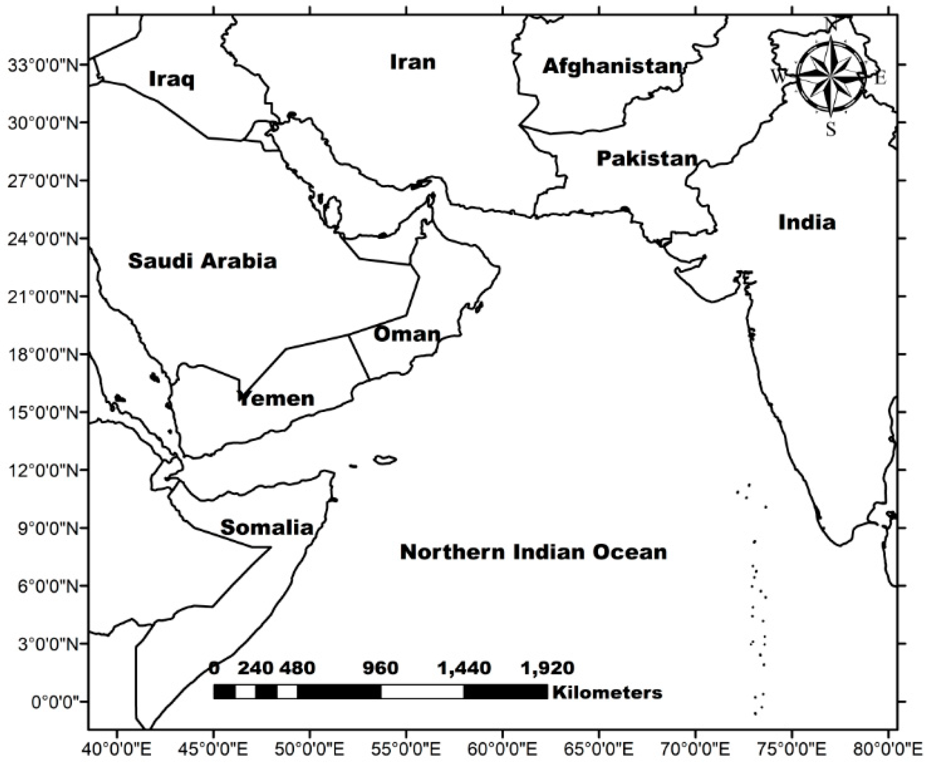
Figure 2.
Time evolution of anomalous (a) 5-day (b) 7-day and (c) 10-day stretch temperature extreme over the land (ATL; black line) and ocean (SST; blue line) in April. The righthand panels are the same as left-hand panels but for May. The µALT and µSST indicate the long-term mean value of the different temperature extremes over land and ocean, respectively.
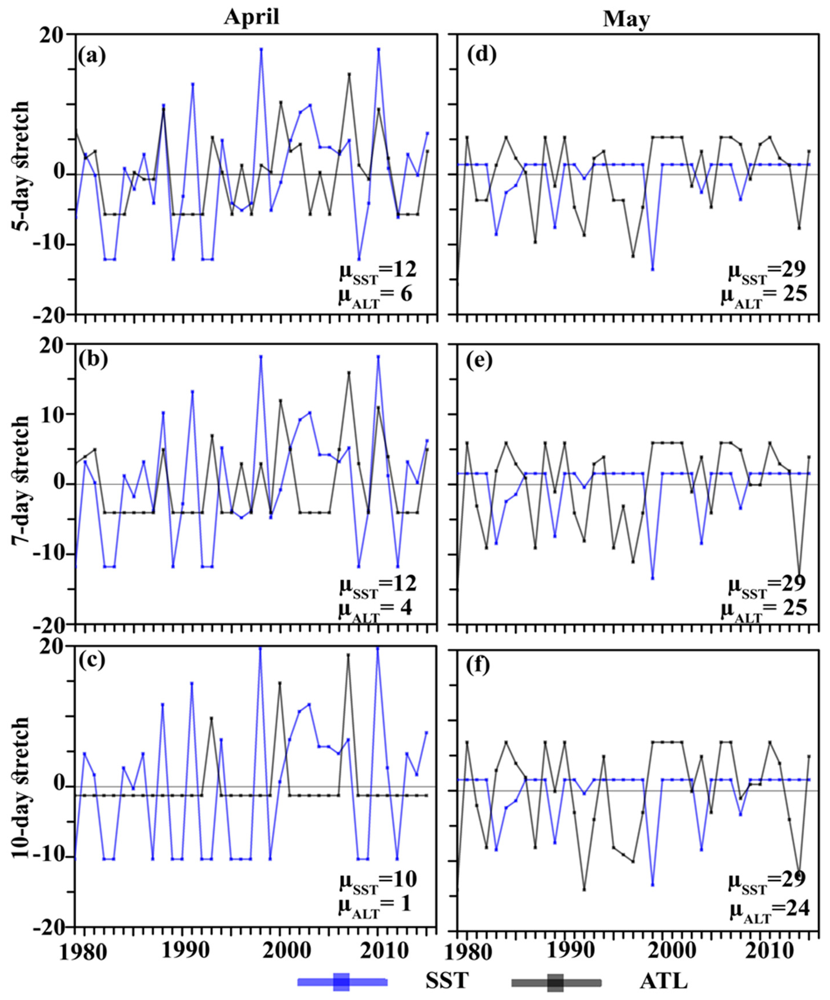
Figure 3.
Time evolution of anomalous (a) 5-day (b) 7-day, and (c) 10-day stretch temperature extreme over the land (ATL; black line) and ocean (SST; blue line) in June. The righthand panels are the same as lefthand panels but for July. The µALT and µSST indicate long-term mean values of the different temperature extremes over land and ocean, respectively.
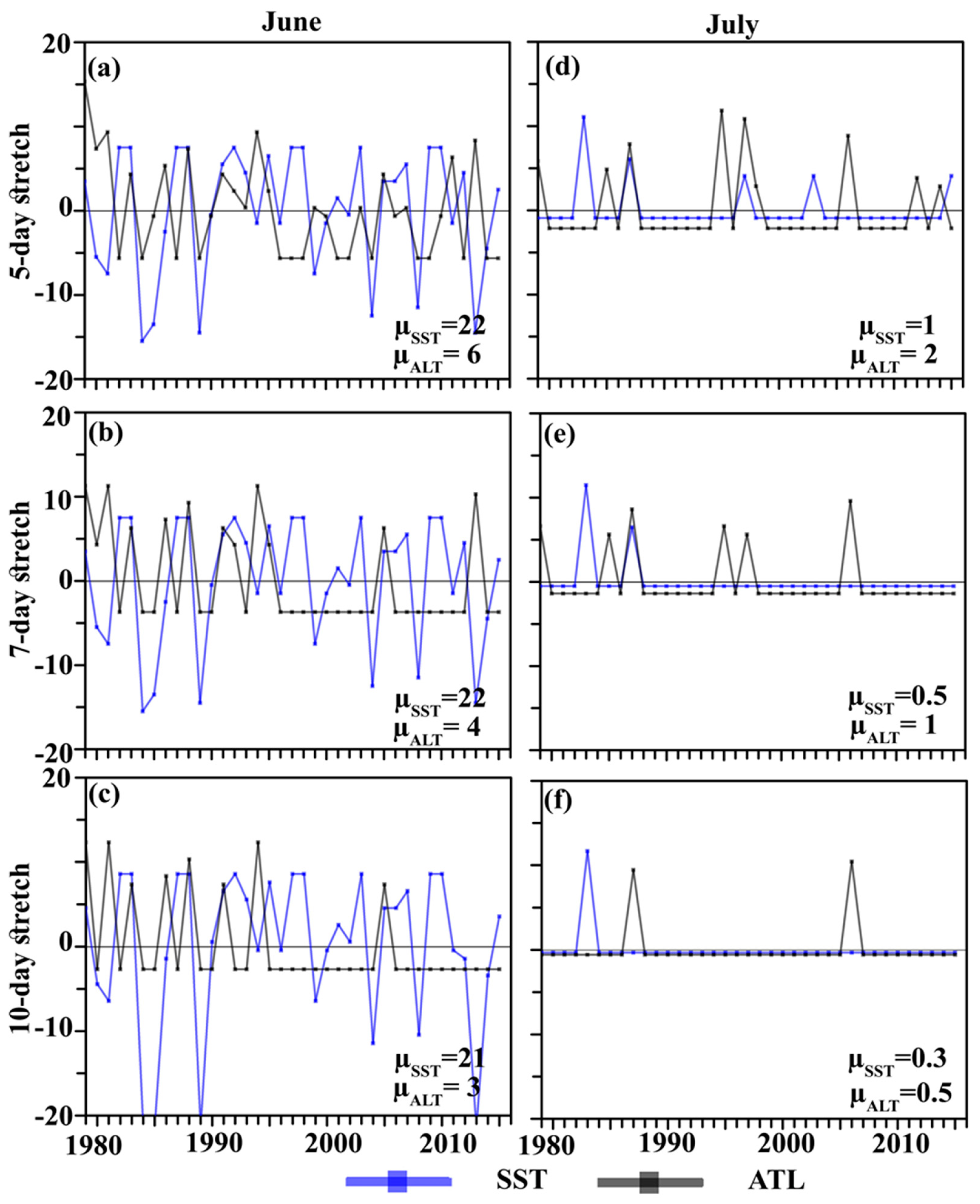
Figure 4.
Time evolution of total events of (a) 5-day (b) 7-day, and (c) 10-day stretch temperature extreme over the land (ATL; black line) and ocean (SST; blue line) in the spring season. The righthand panels (d-f) are the same as lefthand panels but for the summer season. The dashed black and blue lines indicate the trend line of different temperature extremes over land and ocean.
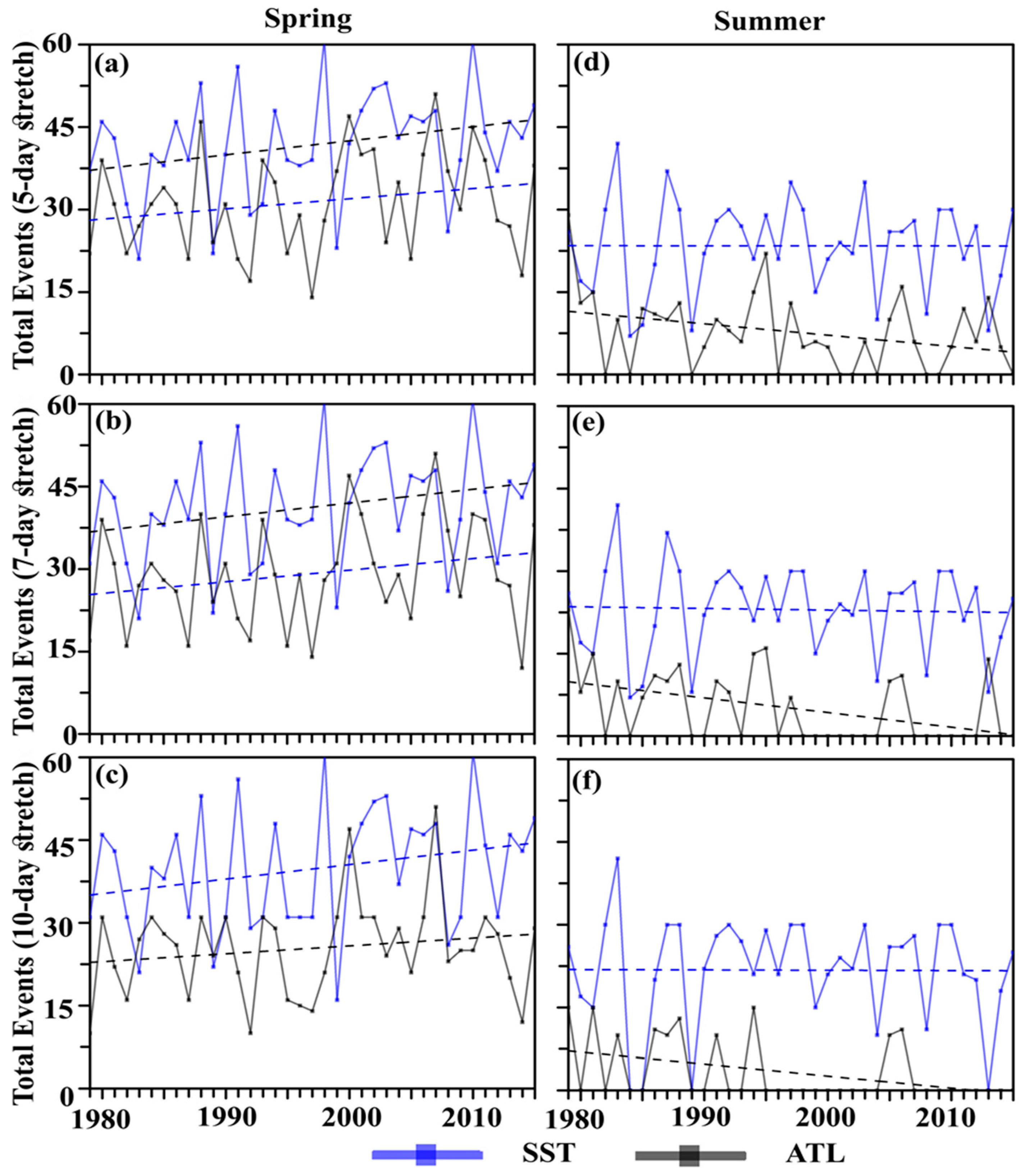
Figure 5.
Range of frequency of temperature extreme anomalies for SST and ATL during 1979-2015 (a) spring (b) summer.
Figure 5.
Range of frequency of temperature extreme anomalies for SST and ATL during 1979-2015 (a) spring (b) summer.
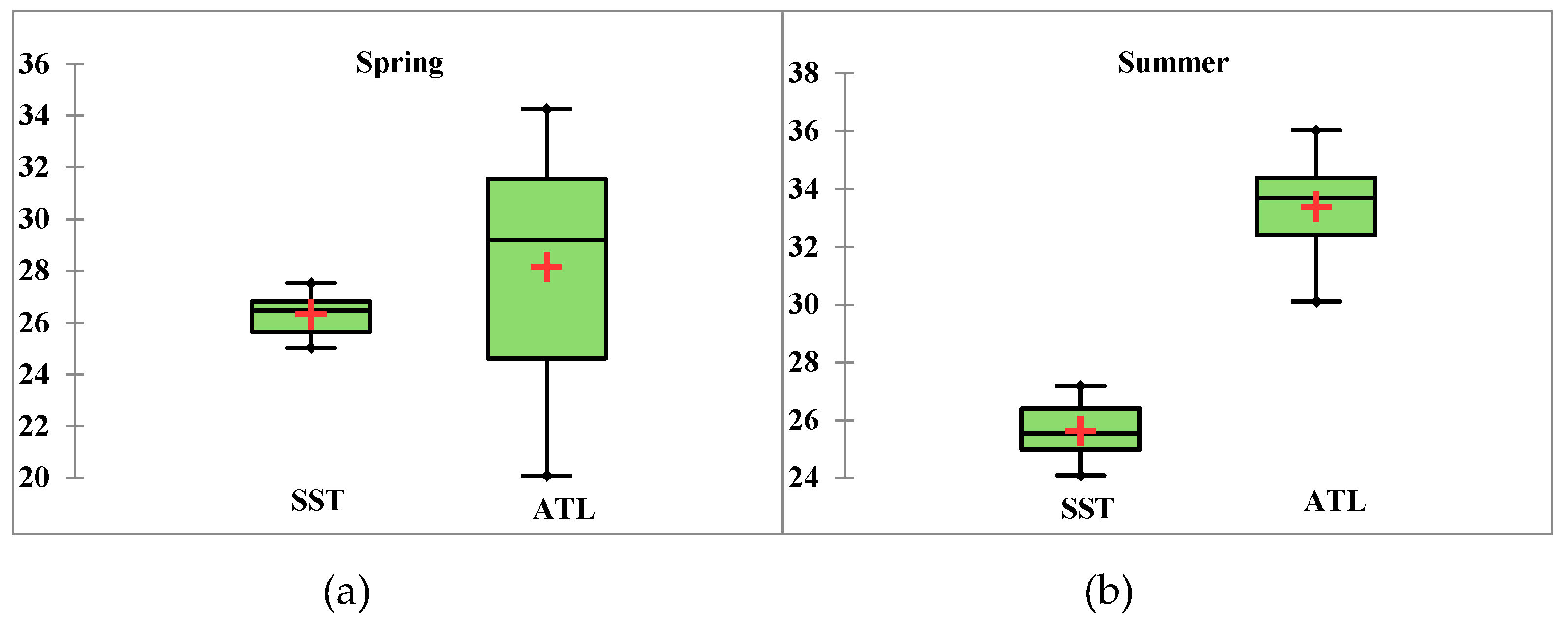
Figure 6.
Regression of temperature extreme events of ATL and SST for (a) spring (b) summer during 1979-2015.
Figure 6.
Regression of temperature extreme events of ATL and SST for (a) spring (b) summer during 1979-2015.
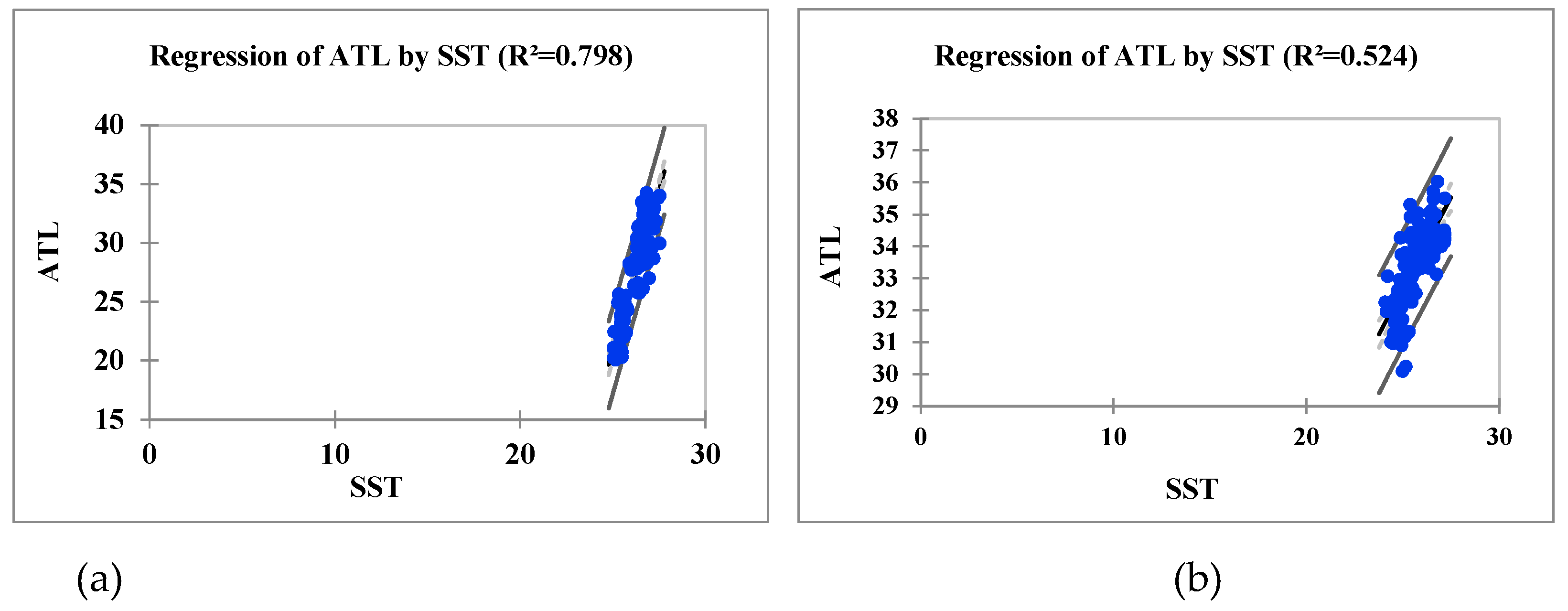
Figure 7.
Spatial distribution of correlation between the NINO3.4 index and 2m temperature over land and ocean in (a) March (b) April and (c) May. The right-hand panels are the same as lefthand panels but for (d) June, (e) July, and (f) August. The contours indicate a statistically significant correlation at a 90% confidence interval.
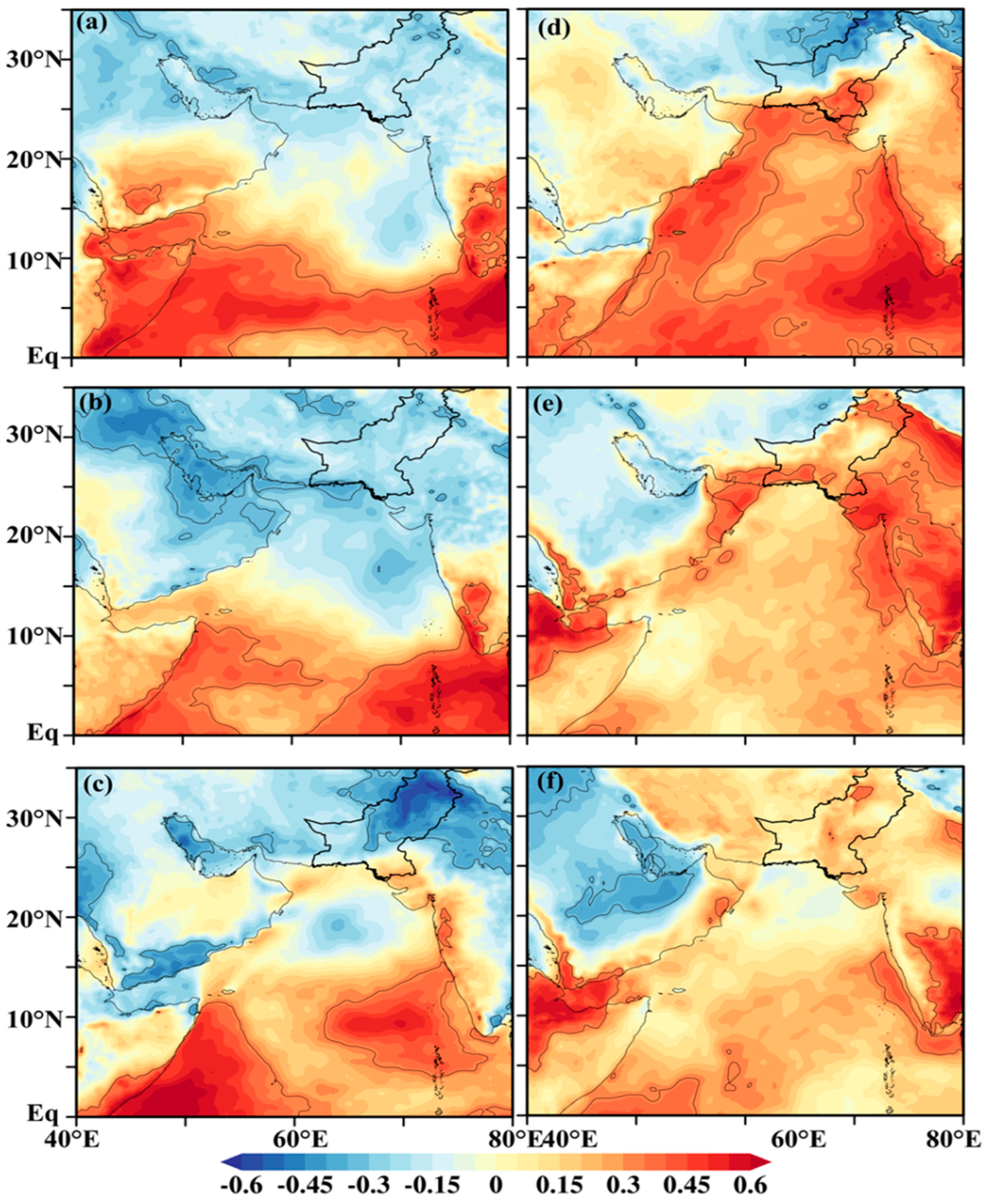
Figure 8.
Spatial distribution of 2m temperature (shaded; ℃) superimposed in 850 hPa wind (vector; ms-1) in (a) spring and (b) summer seasons. Lower panels depict the correlation between the NINO3.4 index and 2m temperature over land and ocean in (c) spring and (d) summer seasons. The contours indicate a statistically significant correlation at a 90% confidence interval.
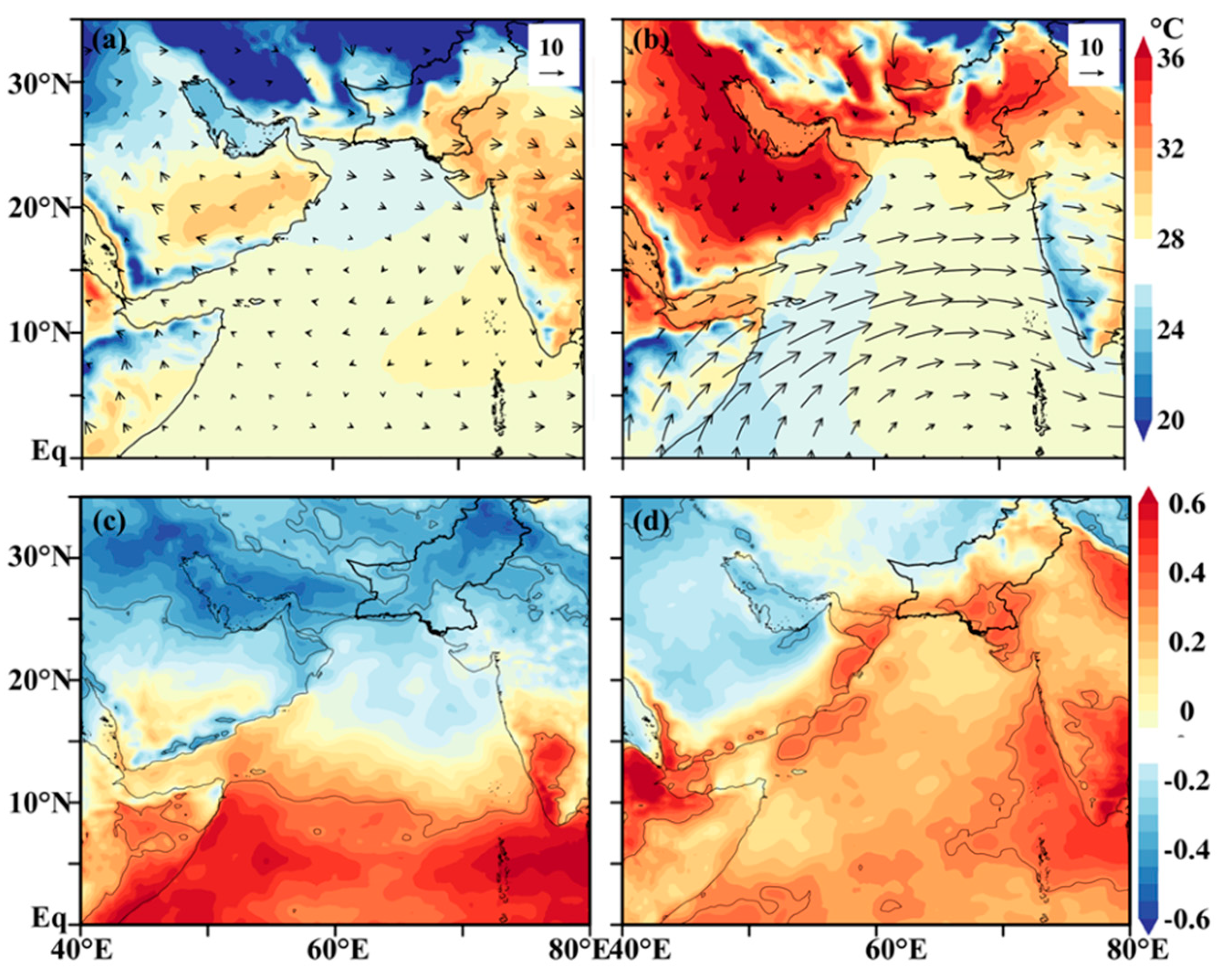
Figure 9.
Spatial distribution of SST (shaded; ℃) (a) spring and (b) summer seasons depicting the correlation between the NINO3.4 index and SST over the ocean on a seasonal basis. The contours indicate a statistically significant correlation at a 90% confidence interval.
Figure 9.
Spatial distribution of SST (shaded; ℃) (a) spring and (b) summer seasons depicting the correlation between the NINO3.4 index and SST over the ocean on a seasonal basis. The contours indicate a statistically significant correlation at a 90% confidence interval.
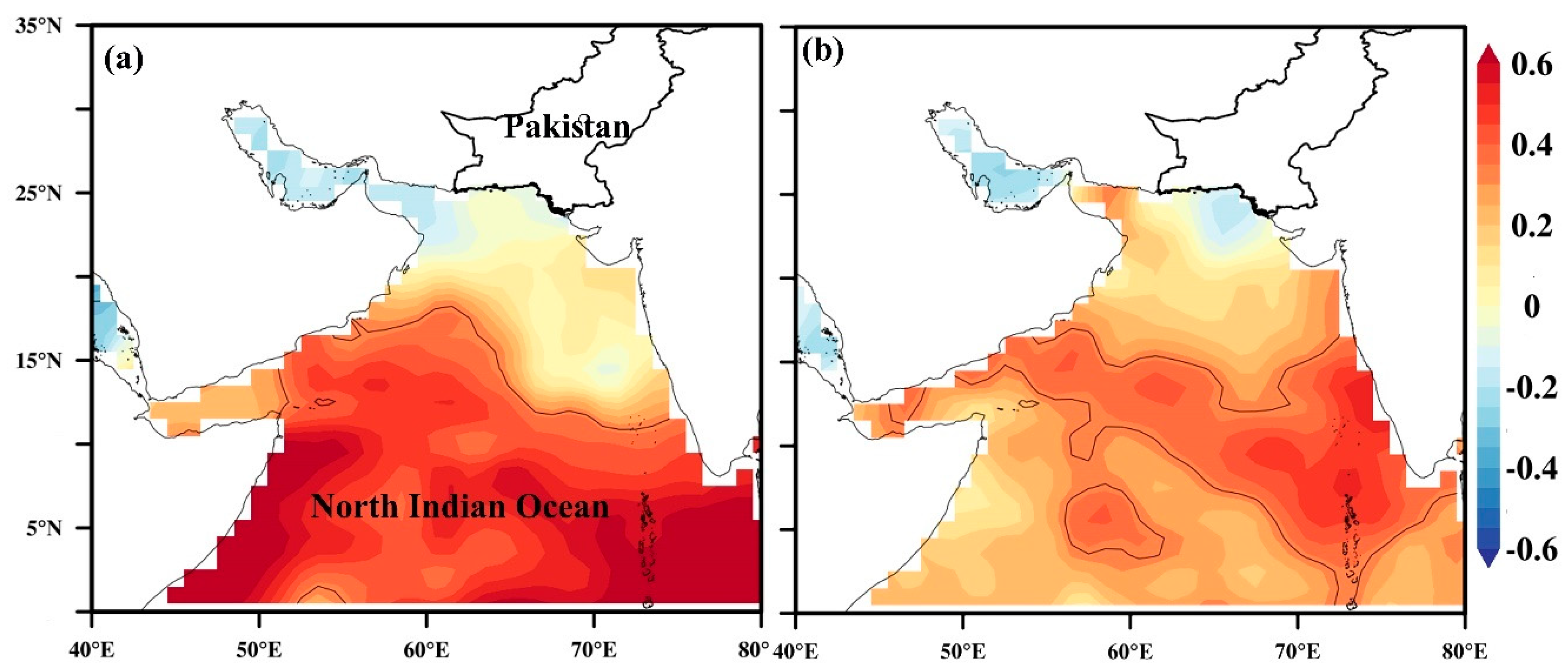
Figure 10.
Spatial distribution of correlation between the NINO3.4 index and SST in (a) March (b) April and (c) May. The right-hand panels are the same as lefthand panels but for (d) June, (e) July, and (f) August. The contours indicate a statistically significant correlation at a 90% confidence interval. .
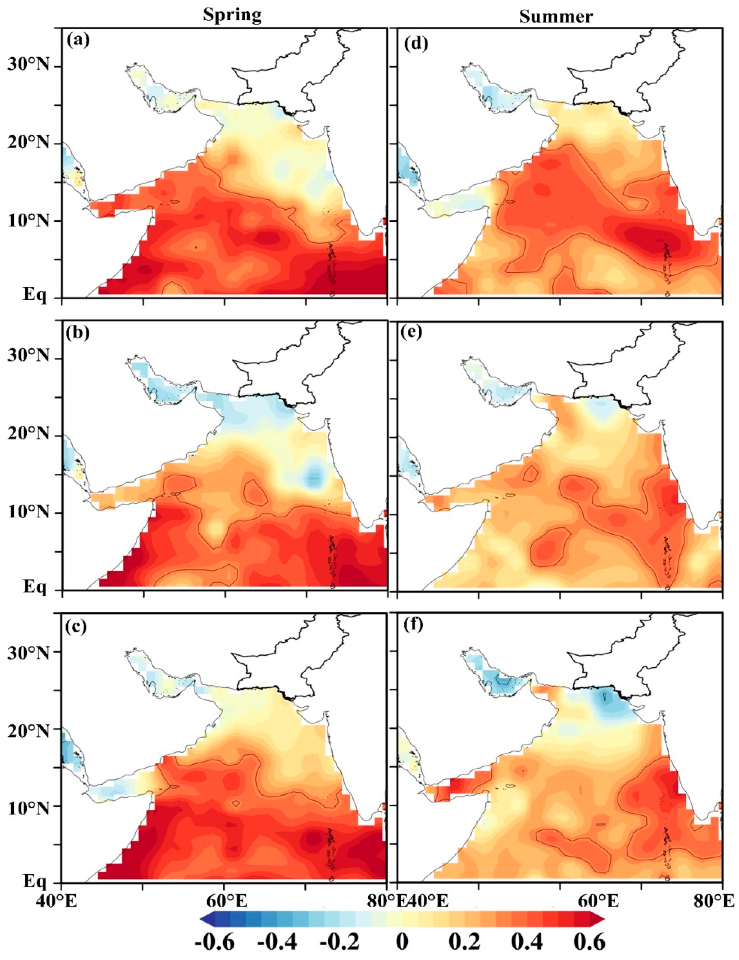

Table 1.
Linear regression analysis of SST and ATL seasonal and monthly temperature extreme events.
|
SST & ATL Thermal extremes |
P-value (Pr>F) |
Ho |
Significance |
R2 |
RMSE |
|
|---|---|---|---|---|---|---|
| SPRING |
Higher Extreme Temperatures |
0.0001<0.05 |
Rejected |
Significant |
0.798 |
1.807 |
| SUMMER |
Higher Extreme Temperatures |
0.0001<0.05 |
Rejected |
Significant |
0.524 |
0.906 |
| APRIL | 5-day Stretch |
0.052>0.05 |
Accepted |
Insignificant |
0.104 |
5.273 |
| 7-day Stretch |
0.136>0.05 |
Accepted |
Insignificant |
0.062 |
5.465 |
|
| 10 day Stretch |
0.907>0.05 |
Accepted |
Insignificant |
0.000 |
4.526 |
|
| MAY | 5-day Stretch |
0.284>0.05 |
Accepted |
Insignificant |
0.033 |
5.607 |
| 7-day Stretch |
0.190>0.05 |
Accepted |
Insignificant |
0.049 |
6.157 |
|
| 10 day Stretch |
0.207>0.05 |
Accepted |
Insignificant |
0.045 |
6.676 |
|
| JUNE | 5-day Stretch |
0.901>0.05 |
Accepted |
Insignificant |
0.000 |
5.870 |
| 7-day Stretch |
0.941>0.05 |
Accepted |
Insignificant |
0.000 |
5.721 |
|
| 10 day Stretch |
0.393>0.05 |
Accepted |
Insignificant |
0.021 |
5.289 |
|
| JULY | 5-day Stretch |
0.334>0.05 |
Accepted |
Insignificant |
0.027 |
4.140 |
| 7-day Stretch |
0.324>0.05 |
Accepted |
Insignificant |
0.028 |
3.235 |
|
| 10 day Stretch |
0.815>0.05 |
Accepted |
Insignificant |
0.002 |
2.442 |
|
Table 2.
Mann-Kendall trend test of frequency of temperature extreme events (SST & ATL) on seasonal basis.
Table 2.
Mann-Kendall trend test of frequency of temperature extreme events (SST & ATL) on seasonal basis.
| MK trend test | Spring | Summer | |
|---|---|---|---|
| Thermal extremes events | Thermal extreme events | ||
| SST | p-value | 0.006 < 0.05 | 0.002 < 0.05 |
| Ho | Rejected | Rejected | |
| Sen’s slope value | 0.009 | 0.015 | |
| Kendall’s Tau (Ʈ) | 0.317 | 0.357 | |
| ATL | p-value | 0.395 > 0.05 | 0.038 < 0.05 |
| Ho | Accepted | Rejected | |
| Sen’s slope value | 0.013 | -0.013 | |
| Kendall’s Tau (Ʈ) | 0.099 | -0.240 | |
Disclaimer/Publisher’s Note: The statements, opinions and data contained in all publications are solely those of the individual author(s) and contributor(s) and not of MDPI and/or the editor(s). MDPI and/or the editor(s) disclaim responsibility for any injury to people or property resulting from any ideas, methods, instructions or products referred to in the content. |
© 2025 by the authors. Licensee MDPI, Basel, Switzerland. This article is an open access article distributed under the terms and conditions of the Creative Commons Attribution (CC BY) license (http://creativecommons.org/licenses/by/4.0/).
Copyright: This open access article is published under a Creative Commons CC BY 4.0 license, which permit the free download, distribution, and reuse, provided that the author and preprint are cited in any reuse.


