Submitted:
28 March 2025
Posted:
29 March 2025
You are already at the latest version
Abstract
Urban development within an urban agglomeration is uneven, and the coordinated de-velopment of urban agglomerations is the core task of urban development. Highway transporta-tion volume is related to urban economic development. By regulating the highway transportation volume of each city in the urban agglomeration, highway collaborative transportation is achieved, thereby achieving coordinated development of the urban agglomeration. According to the characteristics of transportation volume regulation, a two-layer complex network regulation model is proposed. The upper nodes are urban entities, and the lower nodes are highway intersections or toll points. Based on the coordinated development of urban agglomerations, a regulation objective function is set. Due to the many variables and constraints, a hierarchical solution method is adopted. A probability search iteration algorithm is proposed innovatively to solve multivariable, many-to-many allocation problems. Taking provincial urban agglomerations as an example, the process of solving the regulation model and realizing the method is explained. The transportation volume regulation methods and strategies proposed in this study realize the best combination of macro-control and micro-control, static and dynamic control, coordinated development, and collaborative transportation. It is an innovative exploration and research on highway transportation volume allocation and collaborative transportation in urban agglomerations and opens up a new direction for research on the coordinated development of urban agglomerations.
Keywords:
urban agglomeration
; coordinated development
; collaborative transport
; complex network
; transportation volume regulation and control
1. Introduction
Urban agglomeration is generally a regional economic unit, with one or two large cities as core cities. The concept of "agglomeration" means mutual cooperation and coordinated development among cities within urban agglomeration, and it promotes urban agglomeration to obtain greater benefits and faster development than individual cities. A transportation system is the spatial structural skeleton of urban economic development in an urban agglomeration, and it is an important bridge for connection and development between cities. Urban economic development and transportation are interdependent and closely interrelated. Therefore, it has become an important research topic worldwide to coordinate the relationship between urban economic development and transportation, and it is one of the most important and challenging research topics in the field of urban planning and transportation management [1].
Highway transportation is characterized by high flexibility, rapidity, convenience, accessibility, and so on, and it plays an important role in the economic development of urban agglomerations. However, there is a paradox between highway transportation and regional economic development: the more developed the highway transportation, the more unbalanced the regional economic development; in other words, the more unbalanced the development among cities in the urban agglomeration. This results in the phenomenon of ‘the strong are always strong, and the weak are always weak’ [2]. There are two main reasons for the paradox: (1) Convenient transportation can reduce the mobility costs between production factors, so convenient highway transportation in a city will absorb the resources of other cities or regions through a certain gravitational effect, thereby occupying more highway transportation network resources, which in turn restricts the economic development of other cities, resulting in unbalanced economic development [3,4]; (2) For a given highway transportation network within an urban agglomeration, there is a static or dynamic maximum transportation volume, and the transportation capacity and capacity of the transportation network are limited. Owing to the lack of macro-control, each city in urban agglomerations pursues the maximization of its own interests. Therefore, well-developed cities have a large volume of highway transportation, which inevitably occupies the resources of the highway transportation network to the greatest extent, and other poorly developed cities occupy less highway transportation resources. Over time, this has led to unbalanced development among cities [5]. To solve the above paradox, a regulation strategy is needed that can not only optimize the economic development of urban agglomerations and coordinate development between cities, but also maximize highway transportation volume. In other words, coordinated development of urban agglomerations is promoted through highway collaborative transportation.
According to the relevant research literature, collaborative transportation is mainly divided into the following types: (1) Focusing on transportation cooperation between enterprises, logistics service providers, citizens, and management departments, multiple participants or stakeholders, and it can improve transportation efficiency through reasonable planning of transportation routes by sharing resources (such as vehicles, cargo distribution centers, etc.) [6,7,8,9]. (2) Coordinated transportation between different transportation modes, such as relying on highway networks, railway networks, civil aviation, and other methods to explore regional coordinated transportation and regulation strategy [10,11,12,13,14]. (3) Reducing the number of vehicles and the total driving distance required for transportation through logistics cooperation and proposing a multi-echelon transportation method, and achieving vertical cooperation in urban transportation systems [15,16,17,18].
For highway transportation, most research is related to traffic flow and urban transportation planning. (1) The micro traffic flow theory analyzes and models the traffic characteristics of individual vehicles. Most of them are based on the analysis of micro driving behavior and travel behavior characteristics, combined with the complex environment and individual physiological characteristics, to form a simulation model [19]. (2) The meso traffic flow theory describes the randomness and uncertainty of traffic flow, studies the real highway network traffic operation status, and describes traffic flow laws, such as the effectiveness of transportation vehicles, signal control, weather, and environmental impact [20]. (3) Macroscopic traffic flow theory introduces concepts such as vehicle density, flow rate, and average speed to study the dynamic behavior of traffic flow at various locations and moments on a traffic section, and describes the changes in traffic flow along the entire road. Transportation planning mainly focuses on the interaction between transportation and land use [21], coordinated development of transportation and the environment [22], analysis of transportation behavior characteristics, traffic surveys and data analysis [23], transportation demand forecast [24], planning decision support tools and transportation policies [25], etc.
Based on the above analysis, most research works study and analyze transportation organizations, logistics plans, planning actions, etc., according to the correlation between transportation and other elements. To improve the different passenger and cargo transportation systems in urban areas, a coordinated approach is used to connect various elements to reduce the negative impact of transportation development and promote the coordinated development of urban agglomerations. Many scholars have conducted research on urban agglomeration development, highway transportation, etc., and the research contents are rich and diverse, but there are still research blind areas and some problems that need to be solved urgently.
(1) The development of major cities in an urban agglomeration is unbalanced, and coordinated development of urban agglomerations is the top priority. There is a lack of research on promoting the coordinated development of urban agglomerations based on highway transportation volume regulation.
(2) At present, the regulation and control technologies of railway and air transportation systems are relatively mature for research on urban agglomeration transportation networks. There are many studies on multimodal coordinated transportation, such as highways and railways, highways and aviation, and railways and aviation, and few scholars discuss the field of collaborative transportation and regulation and control of highway transportation in urban agglomerations. Whether on expressways or other highways, most vehicles are spontaneously organized and lack macro-control and constraints. Vehicles sent by various cities to highway transportation networks are random and variable. There is a lack of overall consideration of the deployment and diversion of highway traffic flow at a macro level, and there is a lack of research on highway traffic control systems, deployment control systems, traffic flow guidance systems, and their interactions.
For a given highway transportation network, because of the maximum transportation capacity and in order to achieve coordinated development among cities in an urban agglomeration, the basic principle of transportation volume allocation is as follows: trying to take care of slow-developing cities and allow them to obtain as much transportation volume as possible, while fast-developing cities should help slow-developing cities by reducing their own transportation volume. Simultaneously, transportation volume allocation should be scientific and reasonable, and control strategies should have appropriate benefits. Regardless of the allocation strategy and method adopted, it is feasible as long as the above basic principles are met.
First, a simple example is provided to demonstrate the relationship between coordinated development and collaborative transportation among cities. As shown in Figure 1, assuming that there is a segment of an expressway from A to B, the maximum transportation volume is TVmax. The maximum transportation volume sent to the segment by City 1 is T1max, and the maximum transportation volume sent to the segment by City 2 is T2max. City 1 developed better than City 2 did. The problem is because T1max + T2max > TVmax , it will inevitably lead to expressway congestion, and the probability of traffic accidents increases, leading to low transport efficiency and affecting the development of the two cities. How can the transportation volume between the two cities be regulated?
Therefore, certain strategies and methods are required. The basic strategy is as follows. Because City 1 developed better than City 2 did, in order to coordinate the development of the two cities, the reduced volume (∆T1) of the transportation volume of City 1 is larger, and that (∆T2) of City 2 is smaller. The following conditions are satisfied: (T1max − ∆T1) + (T2max − ∆T2) = TVmax and ∆T1 > ∆T2. In this way, City 2 can obtain a relatively large transportation volume, which will naturally promote the development of City 2, realizing the coordinated development of the two cities, and realizing the collaborative transportation of the segment at the same time. On the contrary, if ∆T1 < ∆T2, the development of City 2 is slow, and a small amount of transportation volume is also allocated, which will inevitably restrict the development of City 2 and does not achieve coordinated development.
Second, suppose there are 10000 cars that should be sent to other cities in City 2. Because of highway congestion and regulation strategies, there are only 5000 cars or 9000 cars that are allocated and sent to other cities, and the impact on urban development must be different. The more the transportation volume is allocated, and the more it will fully meet the requirements of urban transportation. If urban transportation capacity increases, it is bound to promote urban development. Therefore, regulation and control strategies for highway transportation volume can promote the coordinated development of urban agglomerations.
The above is a simple example of transportation volume allocation between two cities. For an urban agglomeration composed of multiple cities, the transportation volume allocation strategy and method based on complex network proposed in this study meet the above principles and requirements, which is an innovative research and exploration on highway transportation volume allocation and collaborative transportation in urban agglomerations.
The remainder of this paper is organized as follows. Section 2 introduces definitions and theorem. Section 3 introduces a two-layer complex network model. Section 4 introduces the objective function, constraint conditions, and solution method. Section 5 introduces a case study and simulation. Section 6 provides a summary of this study.
2. Definitions and Theorem
Definition 1:
Matrix comparison.
If A and B have the same number of rows and columns, as the following condition is met, and this is called A > B. Conversely, A < B.
Definition 2:
Matrix dot multiplication.
If A and B have the same number of rows and columns, A is multiplied by B, as the following formula shows; this is called matrix dot multiplication.
Definition 3:
The static shortest transport route.
Among all transport routes from the city i to the city j, the route with the shortest length is called the static shortest route.
Theorem 1:
, when the increase in y is much greater than the increase in x, the value of x is regarded as approximately constant, and the value of the function is decreasing.
Proof:
The partial derivatives of function f(x,y) with respect to x and y:
(1) Because n>0, x>0 and , the value of the function is increasing in the x direction;
(2) Because n>0, y>0 and , the value of the function is decreasing in the y direction.
The change of the value of the function depends on the relative rate and magnitude of the change of x and y, because x<y:
(1) If x is kept constant and y increases, and x<y, the value of f(x,y) will decrease;
(2) If x increases and y increases, x<y, the function value may increase first, and then due to the increase of y, the function value may decrease again. The functional curve in Figure 2 shows this trend.
3. Double-Layer Complex Network Model
A transportation network in an urban agglomeration has the properties of self-organization, self-similarity, and a small world, and it satisfies the characteristics of a complex network. In the field of urban research, multi-layer complex networks are mainly used in transport supply chain path optimization [26,27], urban disaster simulation and vulnerability analysis [28], land use change and land use transformation direction [29], and transportation network structure change [30]. Related research on complex networks mainly focuses on the empirical research of network characteristics [31], detection of network center nodes [32], process of dynamic change and propagation [33], robustness and vulnerability [34,35], and multi-layer network theory and application [36]. There are no related studies on the applications of complex multi-layer networks for the regulation and control of urban agglomeration transportation volume.
According to the characteristics of the urban agglomeration and transportation network, a single-layer urban agglomeration transportation network model GU and a single-layer expressway transportation network model GL are established. The urban agglomeration transportation network model represents the correlation relationship of the transportation volume exchange among multiple cities, and the highway transport network model represents the topological structure of highway transportation networks in urban agglomerations. Subsequently, a double-layer complex network of urban agglomeration transportation model is constructed. Whether it is urban transportation volume exchange or highway transport behavior in the network structure, the relationship between any two points is two-way, and the constructed transportation double-layer network of urban agglomeration is an undirected weighted network.
3.1. Single-Layer Transportation Network Model
3.1.1. Urban Agglomeration Transportation Network Model (GU)
Nodes of urban agglomeration transportation network model GU are major cities and the model is defined as follows:
where is the node set, is the edge set, is the basic node weight, is the node edge weight, and is the adjacency matrix.
(1) Adjacency matrix
Suppose that there are n major cities, and then:
According to the transportation relationship between cities in urban agglomerations, is n * n matrix with element 1.
(2) Basic node weight
The basic node weight , and it is defined as the node transportation intensity:
where is the highway transportation volume of city i, including the sent and received volumes, and is the total transportation volume of an urban agglomeration. Since the sum of the sent volumes of the urban agglomeration is equal to the sum of the received volumes of the urban agglomeration, the denominator of equation (1) needs to be divided by 2 to ensure that the value of is less than 1.
The node transportation intensity reflects the proportion of urban transportation volume in the total transportation volume of the urban agglomeration, which is dynamic. The greater the value is, the stronger the transportation activity of the city is, and it means that there are more connections with other cities. It shows that the greater the basic node weight, the larger the urban transportation volume and the better the urban development. In contrast, urban development is poor.
(3) Node edge weight
The edge weight between two nodes , and it is defined by the proportion of the transported transportation volume between the two cities to the total transportation volume of the urban agglomeration.
where is the sent transportation volume from city i to city j and is the total transportation volume of the urban agglomeration.
The edge weight reflects the degree of transportation between two cities. The greater the weight, the stronger the transportation links; otherwise, the links are weaker. If is known, the following calculation can be obtained.
The sent transportation volume from city i to city j:
The sent transportation volume of city i:
The received transportation volume of city i:
The total sent transportation volume of urban agglomeration:
According to the above relationships, the following matrix operation relationships can be derived.
Set:
Then:
3.1.2. Expressway Transportation Network Model (GU)
Expressway transportation accounts for approximately 80% of urban agglomeration transportation, which is the main highway transport network. An expressway is a closed highway, and only the entrance-exit toll stations are connected to an external road network. Therefore, it is convenient to regulate and control transportation volume, and we mainly study expressway transportation networks.
An expressway transport network is defined as the follows.
where is the node set, is the edge set (road segment set), is the basic node weight, is the node edge weight, and is the adjacency matrix.
The nodes of the model are composed of the following nodes: (1) city toll stations, where a city defines a toll station, and (2) the intersection of one expressway and another expressway, which is the crossing point from one expressway to another.
(1) Adjacency matrix
Suppose that there are m nodes, and then:
If node 1 is the starting point and node m is the endpoint, the adjacency matrix is a m*m symmetric matrix. It can be proved that the upper triangular matrix reflects the forward driving relationship from node1 to node m, whereas the lower triangular matrix reflects the reverse driving relationship from node m to node 1.
(2) Basic node weight
The basic node weight is defined as the node connection degree , which refers to the number of road segments directly connected to the node. reflects the direct connection density between nodes in an expressway network. The larger is, the greater the basic node weight is, which means that more other nodes are connected to it. Therefore, the node is more important.
where is the road segment between node i and node j.
(3) Node edge weight
For the node edge weight between the two nodes (road segment weight) , it is defined as the ratio of the transportation volume per unit time of the road segment to the total transportation volume of the upper urban agglomeration transportation network. The greater the weight, the greater the current transportation volume and the more important the road segment; however, the road segment is also easily congested.
where is the transportation volume per unit time of the road segment and is the total transported transportation volume of the urban agglomeration.
Set the transportation volume matrix of road segments as follows:
and then
Suppose that represents the input transportation volume of node i, represents the output transportation volume of node i, and then:
If there is only one adjacent node from i to j (k=1), then is the transportation volume from i to j. According to the above relationships, the following matrix operation relations can be derived.
Set:
Then:
3.2. Double-Layer Complex Network
A multi-layer complex network is composed of many single-layer networks, and each single-layer networks is connected with each other. Compared to the single-layer network, the multi-layer complex network is closer to the spatial structure of the multi-mode transportation network, and it reflects the heterogeneity of different layer networks. According to the characteristics of the transportation network of urban agglomeration, the single-layer model and are connected to form a double-layer complex network model G of urban agglomeration transportation. As shown in Figure 3, the mathematical model is described as follows:
G is an undirected double-layer complex network, is the upper and lower node connection matrix, , and is the interlayer connection relationship.
and are interlayer edge weight matrix, and its element is the edge weight between the upper node and lower node , which is the static shortest transport route from the upper node to the lower node .
For the convenience of analyzing the problem, the lower toll node number must be consistent with the upper corresponding city number, and the number of adjacent nodes must be as close as possible according to the connection order of the nodes. Therefore, when the node number of the lower layer is equal to that of the same city in the upper layer, the edge weight between the layers expresses the length of the shortest static transport route between the two cities ().
The inter-layer edge weight can be assigned to multiple types of values. For example, it can be defined as the ratio of the transportation volume sent from the upper city node to the lower node () to the total sent transportation volume of the urban agglomeration ():
When the toll node number of the lower layer is equal to that of the same city in the upper layer:
From the relationship between the upper and lower layers of the network, we can see that: (1) the node transportation volume allocation scheme of the upper layer network affects the road segment transportation volume of the lower layer; (2) the capacity of the road segment of the lower layer (maximum transportation volume) and the transport time cost (transport route) constrain the transportation volume allocation scheme between the upper cities; (3) the upper layer network mainly solves the problem of coordinated development among cities in urban agglomeration, and it cooperates with the lower layer network to solve the problem of collaborative transportation of expressway networks.
4. Transportation Volume Regulation Model
4.1. Objective Function and Constraint Conditions
As discussed above, the purpose of transportation volume regulation and control is to balance the transportation volume sent by each city and to promote the coordinated development between cities. On the other hand, the total transportation volume of the urban agglomeration does not exceed the maximum transportation volume of the transport network and ensures that each road segment does not cause congestion. The basic weight of the upper urban node is defined as the node highway transportation intensity , which reflects the transportation volume of the city. The average transportation intensity of the urban agglomeration nodes is calculated as follows:
If the transportation intensity of each city is close to the average value, this is a satisfactory allocation scheme that can realize the requirement of coordinated development. The satisfaction variance is set as the objective function, and the minimum value is considered.
4.1.1. Constraint Conditions of the Upper Layer Network
The total transportation volume of urban agglomeration:
The sent transportation volume of city i:
The received transportation volume of city i:
The sent transportation volume between cities:
where is the minimum sent transportation volume of city i, is the minimum received transportation volume of city i, is the minimum sent transportation volume between cities, andis the total transportation volume of the urban agglomeration.
4.1.2. Constraint Conditions of the Lower Layer Network
According to transportation direction, the lower expressway network is divided into two directional driving networks, which is namely the forward driving network and the reverse driving network. The expressway network can be reconstituted according to the fastest dynamic transport route. Based on the dynamic fastest transport route algorithm [1], the fastest driving route is found from the starting point (corresponding to the upper layer ) to the endpoint (corresponding to the upper), and the fastest forward driving route network is formed. By setting as the starting point and as the endpoint, the fastest reverse driving route network can be obtained. In theory, the structures of the two networks should be the same; they have the same segments but different directions. However, because it is the fastest dynamic route road network, not the shortest static route road network, the structure of the two road networks may be different. We assume that the structures of the two road networks are exactly the same but in different directions.
The fastest dynamic route network is composed of the fastest multiple paths, and there are the same segments between these paths; therefore, the structure of the fastest dynamic route network is simpler than that of the original road network.
The congestion rate OD matrix is set as RC [2], represents the congestion rate of the road segment (between 0-1), and the maximum congestion rate is . The current transportation volume OD matrix is RF and represents the current transportation volume of the road segment. The newly added transportation volume OD matrix is NF, where represents the newly added transportation volume of the road segment. The maximum transportation volume of the road segment in the driving road network is .
Constraint conditions are set as the following.
Equations (21) to (27) are the constraint conditions of the objective function.
4.2. Solving Method for the Objective Function
(1) Objective function analysis
Objective function (21) is transformed into matrix operation, which is convenient for programming.
Because:
Set:
Then:
Based on (7), (8), (9), and (29), the objective function can be calculated by matrix operation.
When n is large (n≥4), in the objective function:
Based Theorem 1, the value of the objective function is decreasing.
Theoretically, there is a global minimum value ( 0 ) for the objective function; that is, the transportation intensity of each city node is equal to the average value. However, it is impossible in actual transportation allocation, and the relative minimum optimal solution can only be obtained: . The objective function (20) has upper and lower layer constraints, and the lower layer constraints are related to the road segment conditions, and there are many constraint conditions and relations. The objective function optimization problem is a multivariable and complex nonlinear optimization problem. If general nonlinear objective function optimization methods are used, such as the Lagrange multiplier method, it involves n* n + k variables (k is the number of constraints). The solution becomes complex when n is relatively large. The simulated annealing algorithm, Gauss-Newton algorithm, and gradient descent algorithm involve solving partial derivatives. The partial derivative of the objective function is not easy to be solved, so it is also very complex.
Based on the regulation and control characteristics of transportation volume, we propose a hierarchical optimization strategy. The basic idea is to optimize the objective function to obtain the transportation volume between cities according to the upper constraints, and then use the lower constraints to regulate the transportation volume and obtain the final transportation volume between cities. A probability iterative algorithm is used to solve the objective function optimization. The probability iterative algorithm is an originally innovative algorithm that is suitable for the optimization of dozens of variables similar to the objective function.
Among the upper constraint conditions, as long as (24) is satisfied, (22) and (23) must be satisfied; therefore, only two constraint conditions are required.
Set:
Then:
Using iterative algorithm, variable iteration:
Converting to weight iteration:
The initial value of transportation volume is set as the minimum transportation volume between cities as:
The initial value of the weights:
The range of weight variation:
Based on (30), the sum of the weights must satisfy the following condition.
Theoretically, if any set of weights satisfies (36) and (37) and the objective function satisfies the following conditions:
Thus, can be considered an effective solution, that is, a Pareto solution. To obtain the optimal efficient solution as far as possible, if the iterative algorithm is adopted, the iterative end conditions should be as follows:
According to the analysis, the total sent transportation volume of a city accounts for approximately 0.4 of the total transportation volume of an urban agglomeration, which is generally a central city. The maximum sent transportation volume between cities accounts for approximately 0.4 of the transportation volume of the city. Therefore, . For the actual calculation, the value is reduced or increased according to the transportation volume requirements of each city.
(2) Probability iteration algorithm
Random search is involved in intelligent optimization algorithms, such as the particle swarm optimization (PSO) algorithm [37], genetic algorithm [38], and evolutionary algorithm [39]. Based on the random search principle and characteristics of transportation volume allocation and regulation, we propose a probability iterative algorithm.
The process of transportation volume allocation can be regarded as a Markov process, and the iterative process of weight is set as follows:
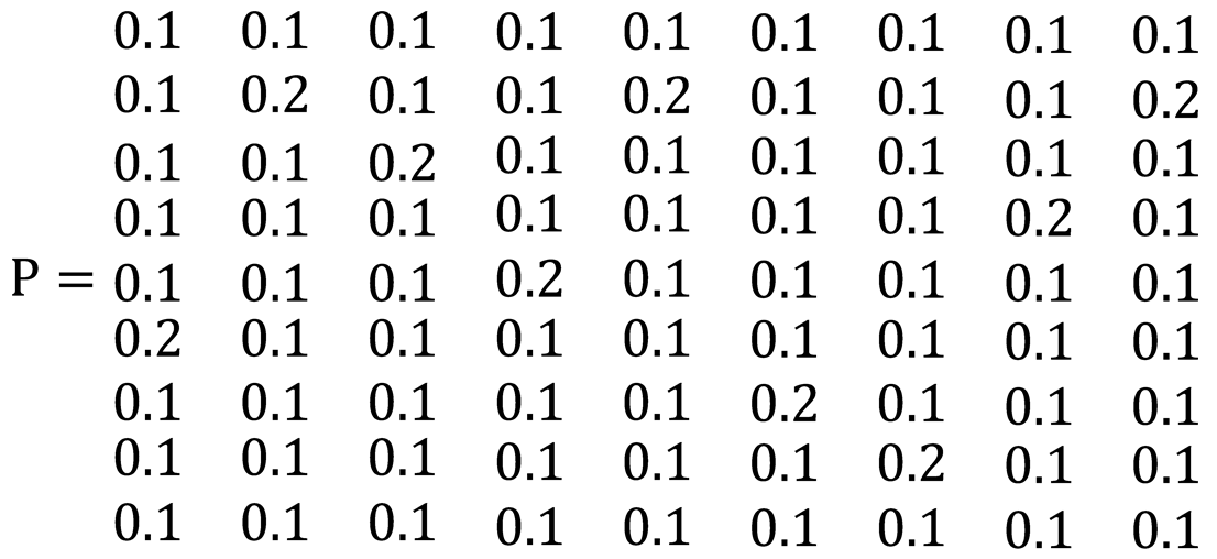
where , m is related to the initial weight value , which is generally 100 or 1000, and is the maximum weight. P is a probability transfer matrix or Markov matrix. As long as the probability transfer matrix P satisfies certain conditions, when the number of iterations k reaches a certain value, (42) eventually reaches a stable state.
P must satisfy the following conditions: (1) P is a random matrix and the sum of all column elements is 1. In other words, , . (2) P is irreducible and the corresponding digraph is strongly connected, that is, there is a path between each pair of nodes. Here, the transportation volume can be allocated between any two urban individuals; thus, the P matrix meets the irreducible requirement. (3) P is aperiodic. Because P is a prime matrix, it is aperiodic.
Based on (42), (43) and Definiton1, because (much less than 1) and , each iteration can be considered as approximating the efficient solution by satisfying the conditions with a small random step based on the initial weight value:
The sum of the weights after each iteration is . Therefore, there exists an efficient solution that satisfies condition (40). According to Theorem 1, , and the efficient solution also satisfies condition (41) in theory. It has been proved by a large number of programming experiments that there is an efficient solution that satisfies the conditions of (40) and (41) simultaneously.
The following conclusions are drawn: For the probability iterative algorithm, there is an efficient solution in the process in which the random search tends to be stable, and it satisfies the end iterative conditions (40) and (41). Even if a solution satisfying the end iteration is not found, the iterative algorithm is convergent, and the final stable solution is also an efficient solution.
The implementation process of probability iterative algorithm is as follows.
Step1. Initial parameter settings, including the total transportation volume of urban agglomeration, minimum transportation volume between cities, maximum transportation volume between cities, iterative parameters (m、δ、β), and probability matrix P;
- Step2.
- Calculate initial weights (), the max weights (), and weight change ();
- Step3.
- Calculate the updated weight () and value of the objective function (;
- Step4.
-
Determine whether the iteration end conditions ((40) and (41)) are satisfied.Yes, go to next step;No, go to Step3;
- Step5.
- End the iteration and output the result.
Taking an urban agglomeration with four cities as an example, the initial conditions are as follows:
The total sent transportation volume of the urban agglomeration: 10000
The initial weights:
The maximum weights:
Iterative parameters: δ=0.1, β=0.01, m=100.
P is set as the following matrix, and the sum of the elements in each column is 1.
The calculation results are as follows. The final weights:
The final transportation volume between cities ():
The total weight: 0.9931, and the total calculated transportation volume: 9931.
The remaining transportation volume: 10000-9931=69.
The transportation intensity of each city: 0.3395, 0.2092, 0.2363, 0.2149.
The value of the objective function: 0.0028.
The calculation results show that the result of the transposed P (, the sum of row elements is also 1) is the same as that of P, and the result of exchanging P between rows or columns is unchanged. When the element value of P is changed, the result remained unchanged. Compared with particle swarm optimization algorithm and genetic optimization algorithm, the final weight, unallocated transportation volume, and transportation intensity of each node are almost unchanged, but there is a slight difference in the transportation volume between cities. The result proves that the probability iterative algorithm is suitable for solving optimization problems with dozens of variables that are similar to transportation volume allocation, and that the programming is simple.
Because of iterative accuracy, the sum of the transportation volume of each city solved by the iterative algorithm may be less than the set total transportation volume, or it may be larger than the set total transportation volume. The remaining transportation volume can be allocated to the slowest developing city or the excess transportation volume can be deducted from the central city.
4.3. Regulation and Correction of Transportation Volume Based on Lower Layer Constraints
Based on (27) and (28), we have:
Therefore,
If , then it should be regulated and the newly added transportation volume should be reduced.
The reduced transportation volume of (adjusted according to the proportion):
After regulation and control, the transportation volume between cities:
The regulated and reduced transportation volume ( can be allocated to some freight that does not need to be sent urgently, which can be transported through national or provincial highways, and reducing expressway transport pressure.
5. Case Analysis and Simulation
We take the regulation and control of expressway transportation volume in the urban agglomeration of Jilin Province in China as an example to illustrate the regulation process, which includes nine major cities: Changchun (CC), Jilin (JL), Baicheng (BC), Songyuan (SY), Siping (SP), Liaoyuan (LY), Tonghua (TH), Baishan (BS), and Yanbian (YB). Figure 4 shows the double-layer network, and Figure 5 shows the lower-layer expressway network. Figure 6 shows the simplified expressway network, which includes nine cities, five expressways, 17 nodes, and 26 road segments. The red nodes are urban toll stations, and the blue nodes represent expressway intersections.
5.1. Transportation Volume Allocation Between Cities
The transportation volume allocation among the nine cities in the urban agglomeration was solved with a total of 81 variables. The probability iterative algorithm was used, and the transportation volume was taken as an integer. The other places were retained four places after the decimal point and five places after the decimal point for the value of the objective function, and a better optimal allocation result was obtained. The value of the probability matrix P was follows, and the sum of each column was 1.
The total weight: 0.9956, and the total calculated transportation volume: 9956.
The remaining transportation volume: 10000-9956=44.
The transportation intensity of each city: 0.1666, 0.1127, 0.1021, 0.1131, 0.0967, 0.1045, 0.0975, 0.098, 0.1087.
The value of the objective function: 0.00042.
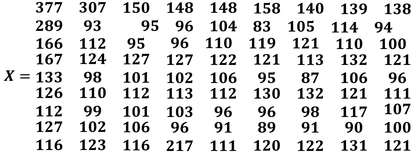
The final transportation volume between cities ():
5.2. Regulation of Transportation Volume Based on Lower Layer Constraints
Figure 7 shows the dynamic fastest route network structure of transportation between cities based on Figure 5. Taking road segment 1-2 as an example, the transportation volumes from Baicheng (BC) to Songyuan (SY), Changchun (CC), Jilin (JL), and Yanbian (YB) are firstly sent through road segment 1-2, so the newly added transportation volume on the segment is as follows:
For road segment 2-1, there is only the transportation volume from Songyuan (SY) to Baicheng (BC), so the newly added transportation volume is .
The calculation method for the newly added transportation volume of other road segments is the same as that of the above road segment 1-2 or 2-1. The sum of the current transportation volume and newly added transportation volume cannot exceed the allowable maximum transportation volume; that is, conditions (26) or (27) should be satisfied. If it exceeds, it must be regulated to meet the constraints.
Taking five cities connected by the G12 expressway as an example, the regulation process is illustrated. At the current time, the OD matrix of the transportation volume sent between cities through the G12 expressway is presented in Table 1.
The road segment setting is shown in Figure 8, the condition settings are shown in Table 2, and the regulation results are shown in Table 2. According to the calculation in reference [1], the number of vehicles on the road segment is between 0 and 250, and the congestion rate is 0 ≤ cr ≤ 0.7.
For example, the newly added transportation volume on the forward road segment is the sum calculated as follows based on Table 1. 121+69+35=225. Current cars: =130, total cars: 225 + 130 = 355. Therefore, the excess volume is 355 – 250= 105, which is the reduced volume. The reduced volume between cities is calculated according to Equation (48).

Table 2.
Conditions and regulation results.
| Forward road segment(A-B) | Reverse road segment(B-A) | |||||||
|---|---|---|---|---|---|---|---|---|
| Name | ||||||||
| 0.7 | 0.7 | 0.7 | 0.7 | 0.7 | 0.7 | 0.7 | 0.7 | |
| Current speed | 90 Km/h |
66 Km/h |
90 Km/h |
90 Km/h |
90 Km/h |
90 Km/h |
80 Km/h |
90 Km/h |
| Estimated cars | 38 | 130 | 86 | 45 | 73 | 68 | 110 | 61 |
| New cars | 90 | 225 | 267 | 32 | 171 | 112 | 287 | 64 |
| Estimated | 0.32 | 0.82 | 0.82 | 0 | 0.69 | 0.54 | 0.86 | 0.29 |
| regulation | No | Yes | Yes | No | No | No | Yes | No |
| Regulated volume | 0 | -105 | -103 | 0 | 0 | 0 | -147 | 0 |
The reduced volume from Jilin to Changchun: 121/225*105=56.
The final volume from Jilin to Changchun: 121 – 56 = 65.
The reduced volume from Jilin to Songyuan: 69/225*105=32.
The final volume from Jilin to Songyuan: 69 – 32 = 37.
The reduced volume from Jilin to Baicheng: 35/225*105=17.
The final volume from Jilin to Baicheng: 35 – 17 = 18.
The calculations of the forward road segment and reverse road segment are the same as above. The regulated and reduced transportation volume can be transported through national or provincial highways or delayed until the road segments are not congested or sent during off-peak hours.
It should be noted that the above data are not accurate real-time data, but mainly explain the regulation process and methods based on the actual situation.
6. Conclusions
The construction of urban agglomerations and their collaborative development are an important part of a country's development, playing an essential role in the economic and social development of the whole country. Urban development in urban agglomerations is unbalanced, which requires collaborative development and mutual support. On the other hand, the resources of highway transport networks are limited in urban agglomerations, and there is a maximum transportation volume; therefore, it is necessary to regulate individual urban transportation volume, allocate traffic volume reasonably, improve transport efficiency, and reduce congestion. This study focuses on the coordinated development of urban agglomerations and collaborative transportation regulation strategies based on highway transportation. This is one of the most important and challenging research topics in the field of urban planning and transportation management, and there is no relevant reference literature yet.
Coordination among cities in urban agglomerations is divided into functional coordination, spatial coordination, industrial coordination, urban-rural coordination, institutional coordination, and so on. This study examines the coordinated development and collaborative transportation of urban agglomerations based on highway transportation regulation, which belongs to functional coordination. It is of great significance to the scientific and rational use of road transport network resources and the realization of coordinated development among cities of urban agglomeration. The main results of this study are as follows: (1) A double-layer network model for regulating the highway transportation volume of urban agglomerations is established using the theory and method of complex networks. (2) An objective function with the weight of the upper urban nodes as variables is established, and the upper and lower constraints are given. (3) Based on the characteristics of the objective function, a probability iteration algorithm is proposed, which is convergent, simple, effective, and convenient for programming. (4) The methods and strategies of transportation volume regulation and control realize an organic combination of macro-control and micro-control, static and dynamic control, coordinated development, and collaborative transportation.
This paper contributes to the research field of coordinated development of urban agglomerations by presenting innovative and practical research. In the future, we will combine the regulation of highway transportation volume with indicators such as urban population growth rate, GDP growth rate, and spatial change rate to study the dynamic simulation of urban development and coordinated development of urban agglomerations, and providing reference for relevant government departments to formulate regional economic development plans.
Author Contributions
Shuoqi Wang: Conceptualization, Methodology, Data analysis, Writing – original draft, Writing – review and editing. Zhanzhong Wang: Writing-review and editing, supervision.
Funding
This work is partially supported by The National Natural Science Foundation of China under Grant 61873109 and the Social Science Foundation of Shaanxi Province in China under Grant 2025QN0471.
Acknowledgments
The authors also gratefully acknowledge the helpful comments and suggestions of the reviewers, which have improved the presentation.
Conflicts of Interest
The authors declare no conflict of interest.
References
- Wang, S, Q. Regulation Strategy of Coordinated Development and Collaborative Transportation for Urban Agglomeration Based on Highway Transportation. Jilin University in China, 2024.
- Wang, S, Q, Wang, Z. Z. Collaborative Development and Transportation Volume Regulation Strategy for an Urban Agglomeration. Sustainability, 2023(20): 14742.
- Song, J.T., Fang, C. L, Song, D. J. Stability analysis of the spatial structure of Chinese urban agglomeration. Acta Geographica Sinica, 2006, 61(12): 1311–1325.
- Fang, C. L., Qi, W. F., Song, J. T. Comprehensive measurement analysis of the compactness of Chinese urban agglomeration. Acta Geographica Sinica, 2008, 63(10): 1011–1021.
- Fang, C. L, Song,J. T, Lin, X. Q. Theory and practice of China’s sustainable urbanization. Beijing: Science Press, 2010, 56–89.
- Xiong, G.; Chen, X.; Shuo, N.; Lv, Y.; Zhu, F.; Qu, T.; Ye, P. Collaborative Optimization of Cyber Physical Social Systems for Urban Transportation Based on Knowledge Automation. IFAC-PapersOnLine 2020, 53, 572–577. [Google Scholar] [CrossRef]
- Li, F.; Guo, X.; Zhou, L.; Wu, J.; Li, T. A capacity matching model in a collaborative urban public transport system: integrating passenger and freight transportation. Int. J. Prod. Res. 2022, 60, 6303–6328. [Google Scholar] [CrossRef]
- Melo, P.C.; Graham, D.J. Transport-induced agglomeration effects: Evidence for US metropolitan areas. Reg. Sci. Policy Pr. 2018, 10, 37–48. [Google Scholar] [CrossRef]
- Wei, G.; Li, X.; Yu, M.; Lu, G.; Chen, Z. The Impact of Land Transportation Integration on Service Agglomeration in Yangtze River Delta Urban Agglomeration. Sustainability 2022, 14, 12580. [Google Scholar] [CrossRef]
- Rong, C. H. From Transport Development to Sustainable Transport. China Railway Science, 2001, 22 (3): 1-8.
- Luo, R. J. Development Ideas of Modern Integrated Transport System in China. China Transportation Review, 2004, 1: 22-25.
- Badada, B.; Delina, G.; Baiqing, S.; Krishnaraj, R. Economic Impact of Transport Infrastructure in Ethiopia: The Role of Foreign Direct Investment. SAGE Open 2023, 13. [Google Scholar] [CrossRef]
- Banerjee, A.V.; Duflo, E.; Qian, N. On the road: Access to transportation infrastructure and economic growth in China. J. Dev. Econ. 2020, 145, 102442. [Google Scholar] [CrossRef]
- Zhao, P. Sustainable urban expansion and transportation in a growing megacity: Consequences of urban sprawl for mobility on the urban fringe of Beijing. Habitat Int. 2010, 34, 236–243. [Google Scholar] [CrossRef]
- Zhao, J.; Li, X.; Lu, H.; Yang, X.; Shen, K. Research on Carrying Capacity of Integrated Transportation in Guanzhong Plain Urban Agglomeration. 19th COTA International Conference of Transportation Professionals. LOCATION OF CONFERENCE, ChinaDATE OF CONFERENCE; pp. 4829–4840.
- Liu, Z.Y, Gao, Y.Y, Wang, J. J. Study on adaptability of urban agglomeration freight transport supply and demand structure based on entropy theory. Proceedings of the 2017 3rd International Forum on Energy, Environment Science and Materials (IFEESM 2017), 2017, 120:1814-1822.
- Liu, Z.Y.; Li, C.B.; Jian, M.Y. Study on the Equilibrium Discriminant Model of Urban Agglomeration Transport Supply and Demand Structure. J. Adv. Transp. 2018, 2018, 1–10. [Google Scholar] [CrossRef]
- Bie, Y. M, Ji Y.T, Ma D.F. Multi-Agent Deep Reinforcement Learning Collaborative Traffic Signal Control Method Considering Intersection Heterogeneity[J]. Transportation Research Part C: Emerging Technologies, 2024, 164: 104663.
- Fang, S.; Yang, L.; Zhao, X.; Wang, W.; Xu, Z.; Wu, G.; Liu, Y.; Qu, X. A Dynamic Transformation Car-Following Model for the Prediction of the Traffic Flow Oscillation. IEEE Intell. Transp. Syst. Mag. 2023, 16, 174–198. [Google Scholar] [CrossRef]
- Zhang, M.; Li, Z.; Wang, X.; Li, J.; Liu, H.; Zhang, Y. The Mechanisms of the Transportation Land Transfer Impact on Economic Growth: Evidence from China. Land 2021, 11, 30. [Google Scholar] [CrossRef]
- Mamede, F.P, da Silva RF, de Brito I Jr, et al. Deep Learning and Statistical Models for Forecasting Transportation Demand: A Case Study of Multiple Distribution Centers]. Logistics-Basel, 2023,7(4):58-69.
- Ghafouri-Azar, M.; Diamond, S.; Bowes, J.; Gholamalizadeh, E. The sustainable transport planning index: A tool for the sustainable implementation of public transportation. Sustain. Dev. 2023, 31, 2656–2677. [Google Scholar] [CrossRef]
- Wang, Z.; Chu, R.; Zhang, M.; Wang, X.; Luan, S. An Improved Selective Ensemble Learning Method for Highway Traffic Flow State Identification. IEEE Access 2020, 8, 212623–212634. [Google Scholar] [CrossRef]
- Shi, Q.; Yan, X.; Jia, B.; Gao, Z. Freight Data-Driven Research on Evaluation Indexes for Urban Agglomeration Development Degree. Sustainability 2020, 12, 4589. [Google Scholar] [CrossRef]
- An, J. Y., Fu ,L., Hu, M,. et al. A novel fuzzy-based convolutional neural network method to traffic flow prediction with uncertain traffic accident information. IEEE Access, 2019, 7:20708-20722.
- Viljoen, N.M.; Joubert, J.W. Multilayered complex network datasets for three supply chain network archetypes on an urban road grid. Data Brief 2018, 16, 1069–1077. [Google Scholar] [CrossRef]
- Viljoen, N.M.; Joubert, J.W. The Road most Travelled: The Impact of Urban Road Infrastructure on Supply Chain Network Vulnerability. Networks Spat. Econ. 2017, 18, 85–113. [Google Scholar] [CrossRef]
- Choe, T.; Kim, J.; Shin, M.; Kim, K.; Kim, M. Complex disaster response framework to reduce urban disaster vulnerability. Sci. Prog. 2023, 106. [Google Scholar] [CrossRef]
- Gomes, E.; Abrantes, P.; Banos, A.; Rocha, J.; Buxton, M. Farming under urban pressure: Farmers' land use and land cover change intentions. Appl. Geogr. 2019, 102, 58–70. [Google Scholar] [CrossRef]
- Dai, L.; Derudder, B.; Liu, X. The evolving structure of the Southeast Asian air transport network through the lens of complex networks, 1979–2012. J. Transp. Geogr. 2018, 68, 67–77. [Google Scholar] [CrossRef]
- Pu, H.; Li, Y.; Ma, C. Topology analysis of Lanzhou public transport network based on double-layer complex network theory. Phys. A: Stat. Mech. its Appl. 2022, 592. [Google Scholar] [CrossRef]
- Cai, B.; Zeng, L.; Wang, Y.; Li, H.; Hu, Y. Community Detection Method Based on Node Density, Degree Centrality, and K-Means Clustering in Complex Network. Entropy 2019, 21, 1145. [Google Scholar] [CrossRef]
- Wang, X.; Tejedor, A.; Wang, Y.; Moreno, Y. Unique superdiffusion induced by directionality in multiplex networks. New J. Phys. 2021, 23, 013016. [Google Scholar] [CrossRef]
- Kumar, S.; Mallik, A.; Sengar, S.S. Community detection in complex networks using stacked autoencoders and crow search algorithm. J. Supercomput. 2022, 79, 3329–3356. [Google Scholar] [CrossRef]
- Yu, A.; Wang, N.; Wu, N. Scale-Free Networks: Characteristics of the Time-Variant Robustness and Vulnerability. IEEE Syst. J. 2020, 15, 4082–4092. [Google Scholar] [CrossRef]
- Milano, M.; Guzzi, P.H.; Cannataro, M. Design and Implementation of a New Local Alignment Algorithm for Multilayer Networks. Entropy 2022, 24, 1272. [Google Scholar] [CrossRef]
- Liu, J.; Zhang, H.; He, K.; Jiang, S. Multi-objective particle swarm optimization algorithm based on objective space division for the unequal-area facility layout problem. Expert Syst. Appl. 2018, 102, 179–192. [Google Scholar] [CrossRef]
- Abdullah, K., David, W. C., Alice, E. S. Multi-objective optimization using genetic algorithms: A tutorial, Reliability Engineering & System Safety, vol.91, no.9, pp.992-1007, 2006.
- Ruhul, S., Liang, K.H., Newton, C. A new multi-objective evolutionary algorithm, European Journal of Operational Research, vol.140, no.1, pp.12-23, 2002.
Figure 1.
Segment of an expressway.
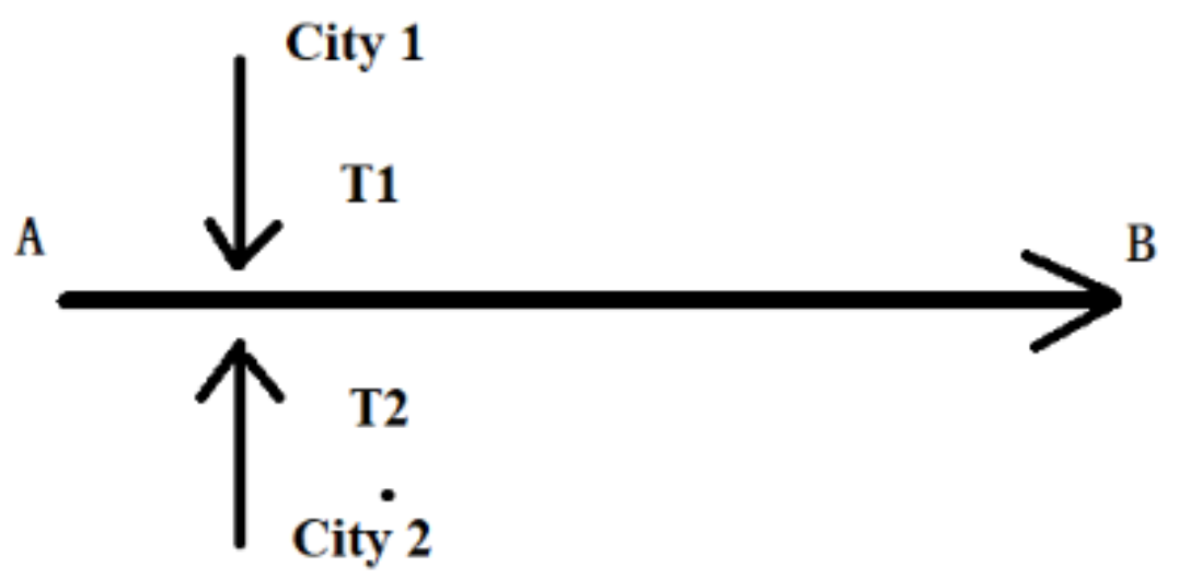
Figure 2.
Functional curve.
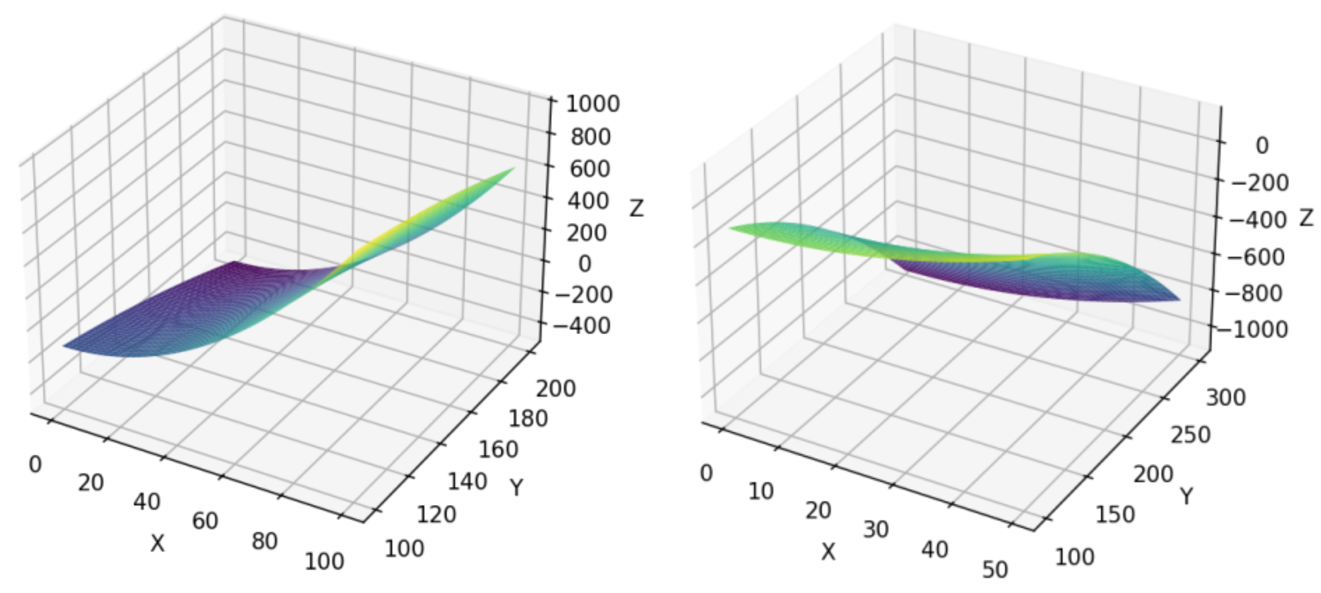
Figure 3.
Double-layer complex network of urban agglomeration transportation.
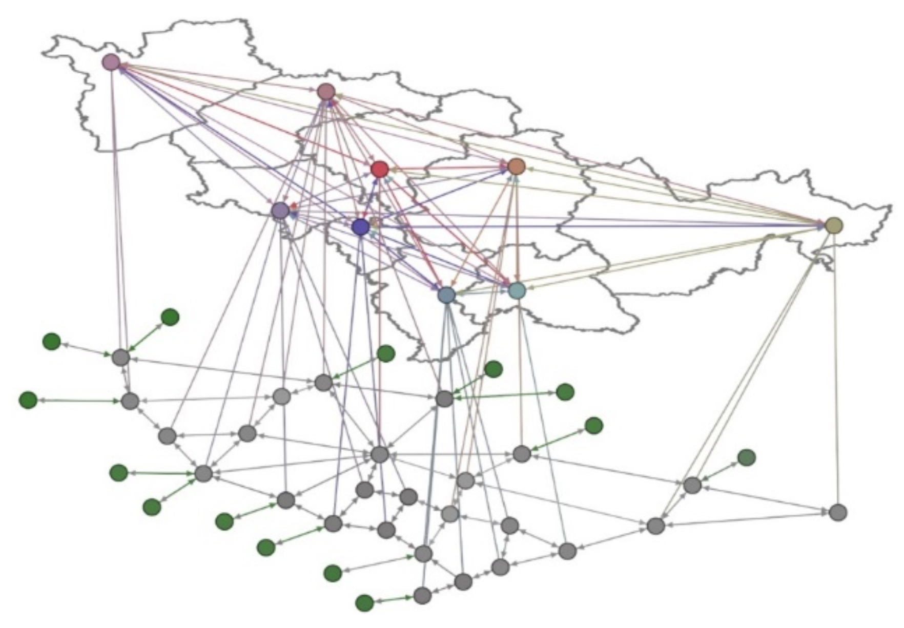
Figure 4.
Double-layer network of the urban agglomeration.
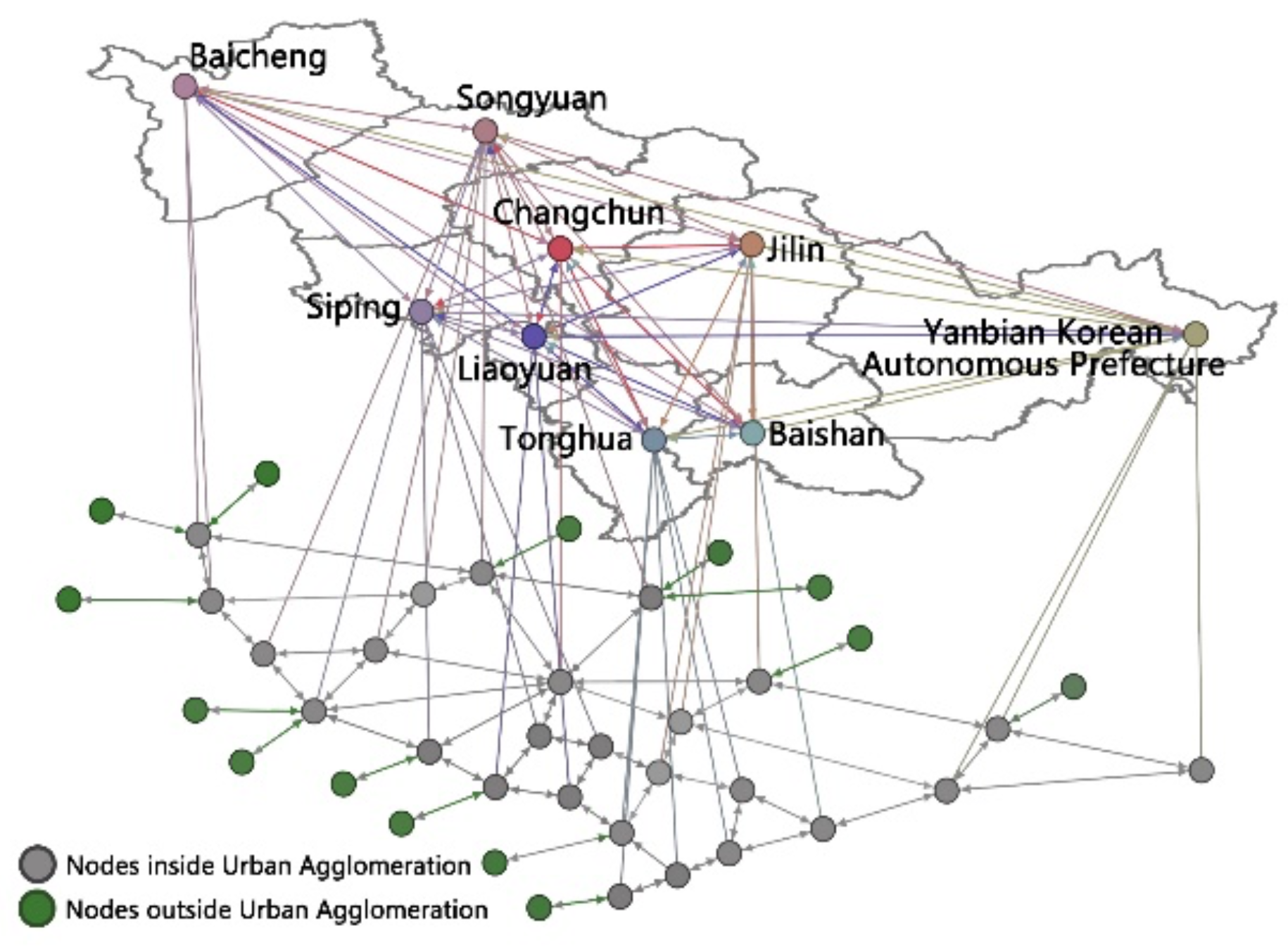
Figure 5.
Expressway network of the urban agglomeration.

Figure 6.
Simplified expressway network of the urban agglomeration.
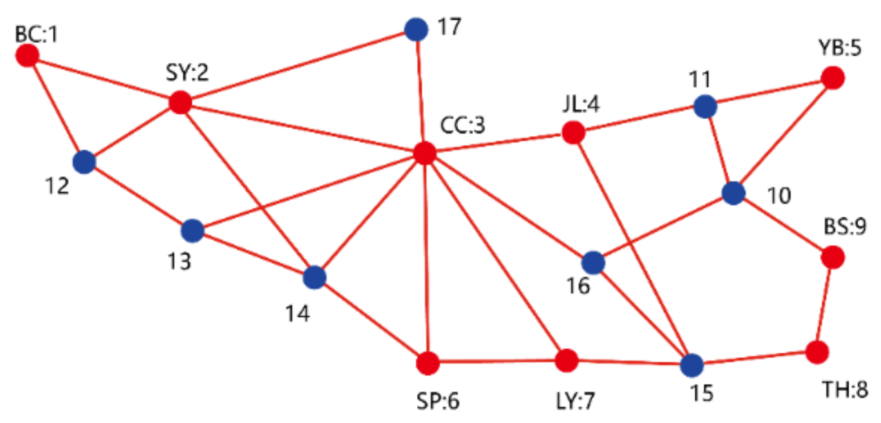
Figure 7.
Dynamic fastest route network of the expressway network.
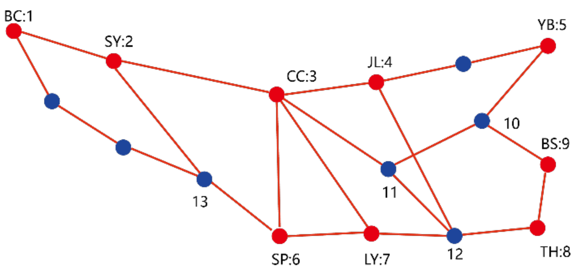
Figure 8.
Road segments of G12 expressway.
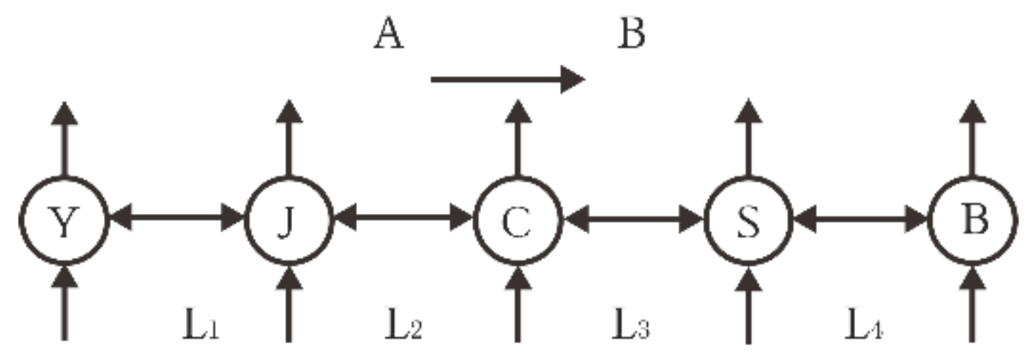
Table 1.
Transportation volume sent between cities.
| City | YB | JL | CC | SY | BC |
|---|---|---|---|---|---|
| YB | 0 | 21 | 38 | 12 | 19 |
| JL | 38 | 0 | 121 | 69 | 35 |
| CC | 48 | 239 | 0 | 146 | 121 |
| SY | 16 | 48 | 21 | 0 | 32 |
| BC | 19 | 32 | 38 | 71 | 0 |
Disclaimer/Publisher’s Note: The statements, opinions and data contained in all publications are solely those of the individual author(s) and contributor(s) and not of MDPI and/or the editor(s). MDPI and/or the editor(s) disclaim responsibility for any injury to people or property resulting from any ideas, methods, instructions or products referred to in the content. |
© 2025 by the authors. Licensee MDPI, Basel, Switzerland. This article is an open access article distributed under the terms and conditions of the Creative Commons Attribution (CC BY) license (http://creativecommons.org/licenses/by/4.0/).
Copyright: This open access article is published under a Creative Commons CC BY 4.0 license, which permit the free download, distribution, and reuse, provided that the author and preprint are cited in any reuse.


