Submitted:
27 March 2025
Posted:
27 March 2025
You are already at the latest version
Abstract
Dielectric relaxation (DR) plays a critical role in understanding interactions between defects and dipoles in materials applied a time-varying electric field. Based on the observations during the DR experiment, intrinsic quantities of materials are extracted typically by exponential-like decay functions. However, these traditional methods involve the rigid constraint of mathematical models and the ill-posedness of inverse calculation, and thus lead to an ambiguous physical meaning of parameters and even failing in parameter estimations from noisy observations. In this paper, a forward method with the learnable current of defects is proposed to extract the physical quantities of DR like time constant, activation energy, defect number, and dielectric loss, where the defect current is learned by a recurrent neural network (RNN) with a cell of shallow multilayer perceptron (SMP) for solving the defect diffusion-controlled chemical reaction equation. After presenting the defect diffusion-informed RNN framework, the efficient architectures are discussed by utilizing TensorFlow-based implementations; and then, validation studies compared with the well-known analytical solution are performed; finally, the robustness and the generalization ability are demonstrated according to the experimental DR data in semiconductor devices. The suggested methodology provides a better DR analysis for discovering hidden physics in emerging materials and devices.
Keywords:
Dielectric relaxation
; defect diffusion
; recurrent neural network
; robustness and generalization
1. Introduction
Dielectric relaxation (DR) is the momentary delay (or lag) in the dielectric constant of a material, which is usually caused by the delay in molecular polarization with respect to a changing electric field in a dielectric medium. The analysis of DR plays a crucial role in investigating the relationship between the structure and the dynamics of charge in diverse materials. The Havriliak –Negami portrayal for dynamics based on the Broadband Dielectric Spectroscopy (BDS) analyzers is the essential tool in the frequency domain for dielectric relaxation analysis. But it is very difficult for frequency-related impedance studies down to micro-Hz range which sometimes needs weeks, and even reliable temperature stabilization for a macroscopic sample is challenging. Whereas, the parameters of DR can be extracted from the observed data in time domain by the fitting model such as exponential expressing Debye-type relaxations [1], and thus coming into a well-established dynamic technique for quantifying the interaction of dipoles and defects in DR processes and widely used in explorations such as in GaN devices [2], molecule junctions [3], as well as electrode-ionic liquid interfaces [4].
Great efforts have been made by numerous empirical researchers to fit the N-length time series data, , with a stretched exponential called Kohlrausch-Williams-Watts (KWW) function [1]-[4],
An important application of the KKW model is to determine the glass transition temperature (Tg), a concept originally developed and applied for synthetic polymers, when describing the relaxation behavior of glass-forming liquids and complex systems [13]. Meanwhile, the KWW function has also been applied to fit various experimental data from mechanical, NMR, enthalpic, volumetric, magnetic relaxation, etc. [11,12], to characterize concisely the transient dynamics and predict their stability by the power exponent (‘stretched’) α and the ‘stretched’ relaxation time τ. Unfortunately, parameters of the empirical model are physics agnostic, which means α and τ cannot be directly related to the characteristics reflecting physical mechanism among the experimental data. To obtain interpretable parameters, a weighted sum of M-term exponentials stating a superposition of Debye-type relaxations is widely utilized [4],
where and denote the relaxation time and the amplitude respectively for the j-th component of Debye-type relaxation which modeling each of the characteristics of the experimental data. However, fitting the sum of exponential functions is an ill-posed problem [5], and thus restrictions is applied to the derivative-based algorithm to directly fit the data with Eq. (2) in finding its optimal parameters. As a reliable alternative to the fit of Eq. (2), the inverse Laplace transform (ILT) [6] of Eq. (1) is employed to obtain the spectrum of relaxation time, ,
where the discrete difference and the profile or the asymptotic [2]. For example, the ILT-based method Eq. (3) accurately captures the distribution of Eq. (1) when [6]. From the viewpoint of random walk of defects, in fact, the empirical model Eq. (1) can be interpreted by the rate equation for defect diffusion-controlled chemical reaction [1],
where denotes the concentration of defects, current of defects , is the gamma function.
Despite its fruitful applications to analyze DR using the exponential based on least-square method, the extraction of DR parameters strongly relies on the inverse process of observed data in rigidly defined models. Especially, the artificial oscillatory components are introduced when the signal-noise-ratio (SNR) of training data is smaller than 40 [6]. Consequently, the available methods for DR analysis are less likely to handle the pending issues covering the ill-posed problem, noisy or truncated data, even for prediction of new physical rules. Recently, there is a trend to apply physics-informed neural networks (PINN) to solve the inverse problem, even to discover hidden physics in various scenarios involved a physical system and some observational data [7,8]. For instance, the prediction of material fracture growth is well demonstrated by combining a recurrent neural network (RNN) with a physics-based crack length increment model [7]. The review [8] summarizes potentials and challenges of the state-of-the-art PINN for diverse physics applications and shows that the choice of the PINN architecture remains an art for many scientific problems. Inspired by the PINN and its ability of forward calculation to approximate solution of partial differential equation, in this paper, a new method for extracting DR parameters is proposed, in which DR is expressed by a first order differential equation with a learning term for the defect current, and furthermore the physical parameters of DR are extracted by the PINN-based forward procedure instead of relying on the traditional inverse calculation. To the authors’ knowledge, little report is given to study the DR by means of PINN so that the pending issues of the traditional DR method can be addressed.
The goal of this paper is to seek a physical model with the forward calculation, accurate prediction, and better interpretability of DR suffering from noises and low resolutions. First, a specific PINN framework for DR is described, where the rate equation expressing the defect diffusion is encoded in the RNN handling time-dependent observations; By implementing forward algorithm using the TensorFlow library, then, the efficient architecture for DR analysis is searched considering the number of layers, form of activation functions, training algorithms, and number of training samples; Next, the validation of the suggested is given considering the relaxation-related spectrums with respect to noises and defects; Finally, a brief conclusion has been made.
2. Framework of Defect Diffusion-Informed RNN
2.1. First Order Difference Equation with Term of Defect Current
It is known that defects like vacancies, grain boundaries, dangling bonds trigger the DR phenomena [1]. The first order differential equation expressing defects diffusion-controlled chemical reaction determines the decay of experimental data in Eq. (4),
that’s,
where the reaction rate . can be predicated when is determined from the prior observations and the given defect currents . However, is a hidden physical quantity such as in Eq. (4), where is related with the step and the pausing-time distribution when defects visit new lattice sites.
To learn the hidden defect current from the observations, furthermore, a shallow multilayer perceptron (SMP) [14,15] is adopted to model in Eq. (6),
and the weights and biases of SMP are estimated by minimizing the loss function such as the mean squared error (MSE),
where denotes the predicated by combining Eq. (7) with Eq. (6) according to the observations . Therefore, the interpretable defect current is learned from the trained SMP or .
2.2. RNN with Cell of SMP for Defect Current
To march Eq. (6) in time , RNN calls a cell ‘Cell-n’ to transform a state and an input at the specific observation index so that the next state and output are generated, seeing Figure 1. The main three units for DR analysis are as follows:
- Prediction by the forward calculation. For the first loop or , the initiate state is set to 1 due to the normalized of decay data of DR, and is the input, first. Then, the instance of cell ‘Cell-1’ makes a feed forward calculation by means of an SMP with dense layers to generate the hidden defect current-related parameter in Eq. (7), where the weights and biases of SMP are initialized from the typical defect current in Eq. (4). Next, the prediction is generated according to Eq. (5) as the output and next state for the second loop. Finally, the above-stated procedure for predictions is repeated for N-1 times until the trajectory of predictions is obtained.
- Optimization of SMP. According to Eq. (8), the loss accounts for the metrics such as MSE to quantify the difference between observations and predictions, and optimizers such as the adaptive momentum algorithm (Adam), quasi-Newton method (L-BFGS) are used to optimize the weights and biases of SMP to satisfy the error of less than a given threshold such as .
- Extraction of DR spectrum. The optimal SMP model approximates the hidden variable , and thus leads to represent the intrinsic defect current or a typical component in Eq. (1) towards the extraction of DR parameters such as the relaxation time spectrum, .
Based on the framework of integrating the defect current equation into RNN, the SMP becomes a parametric neural network with learnable activation, which can be trained for the solution of the defect current in Eq. (5). And this indicates that the typical inverse problem of DR analysis is transformed to the forward calculation scheme through optimizing the SMP’s hyper-parameters with respect to the observed data and the defects diffusion-controlled chemical reaction.
3. Efficient Architecture for DR Data
In this section, the TensorFlow-based Python implement for the proposed framework is illustrated and the choice of architecture is discussed to balance the trade-off between the error of loss function and the accuracy of RS analysis.
3.1. Implementation
Considering the fruitful libraries and available repositories for the artificial neural network implementation [7,8], the framework of defect diffusion-informed RNN is programmed by means of Python language and TensorFlow library. The pseudocode is given in Table 1.
For the observations generated through Eq. (1) at and , they can also be derived from Eq. (4) with the defect current , seeing Figure 2 (a), where the observation, the defect current, and the hidden variable in Eq. (6) or ‘dR’ are shown.
Based on the generated observations, the data of at an arbitrary exponent such as 0.7 is used as the training dataset in Eq. (7) during the initiation of weights and biases of SMP. After 200 epochs, outputs of the initiated SMP or ‘initial fitting-dR’ and the training data or 'initial setting-dR’ are shown in Figure 2 (b), and the loss between them is less than . Hence, the SMP constructed by 3-layer perceptron with full connections has a good expressivity of . In addition, the learnable ability for hidden variable is investigated by training the proposed RNN with the above initiated SMP. The loss is after 200-epoch forward predictions according to 200 observations from Eq. (1) at . Figure 2 (b) illustrates the trained or ‘trained dR’ from the initial or ‘initial fitting-dR’, and compares with the ‘ideal dR’ using the theoretical defect current , and moreover, there is a nearly linear relationship between the trained and the ideal as shown in the inset of Figure 2 (b).
Besides the demonstration of expressivity and learnability of the hidden variable, outputs or predictions of the proposed method are compared with the inputs or ideal observations. Figure 2 (c) shows that the predictions before and after training or ‘Before training’ and ‘After training’, where ‘Before training’ denotes the prediction of the proposed method only using initialization of hyperparameters, and they are compared with the ideal observations or ‘Ideal’. The result shows that the predictions after training are in line with the ideal observations except the deviation occurred at the data tail. Based on the learned defect current, furthermore, relaxation time spectrums at exponent α=0.5,0.7,0.98 in Eq. (3) are demonstrated in Figure 2 (d), which means that the greater the exponent is, the narrower the spectrum is. Therefore, the analysis of typical decay functions can be reached by the proposed forward scheme instead of the traditional inverse method.
3.2. Optimal Choice of Architecture
Although the small loss of about is obtained by the implementation of default architecture in Table 1, there is still an obvious difference between the prediction and the ideal, especially in the data tail such as the data range for time greater than 2 in Figure 2 (b)(c). To address this issue, the optimization of the architecture is conducted by the empirical method due to the lack of the theoretical strategy. Based on the default architecture involved four primary factors: 200 epochs, 5 layers of dense, tanh activation function, root-mean-square propagation (RMSprop) optimizer, the parameter for each factor is changed to the available values or selections in the library. The influences of separate changes in factors of the architecture are investigated as follows.
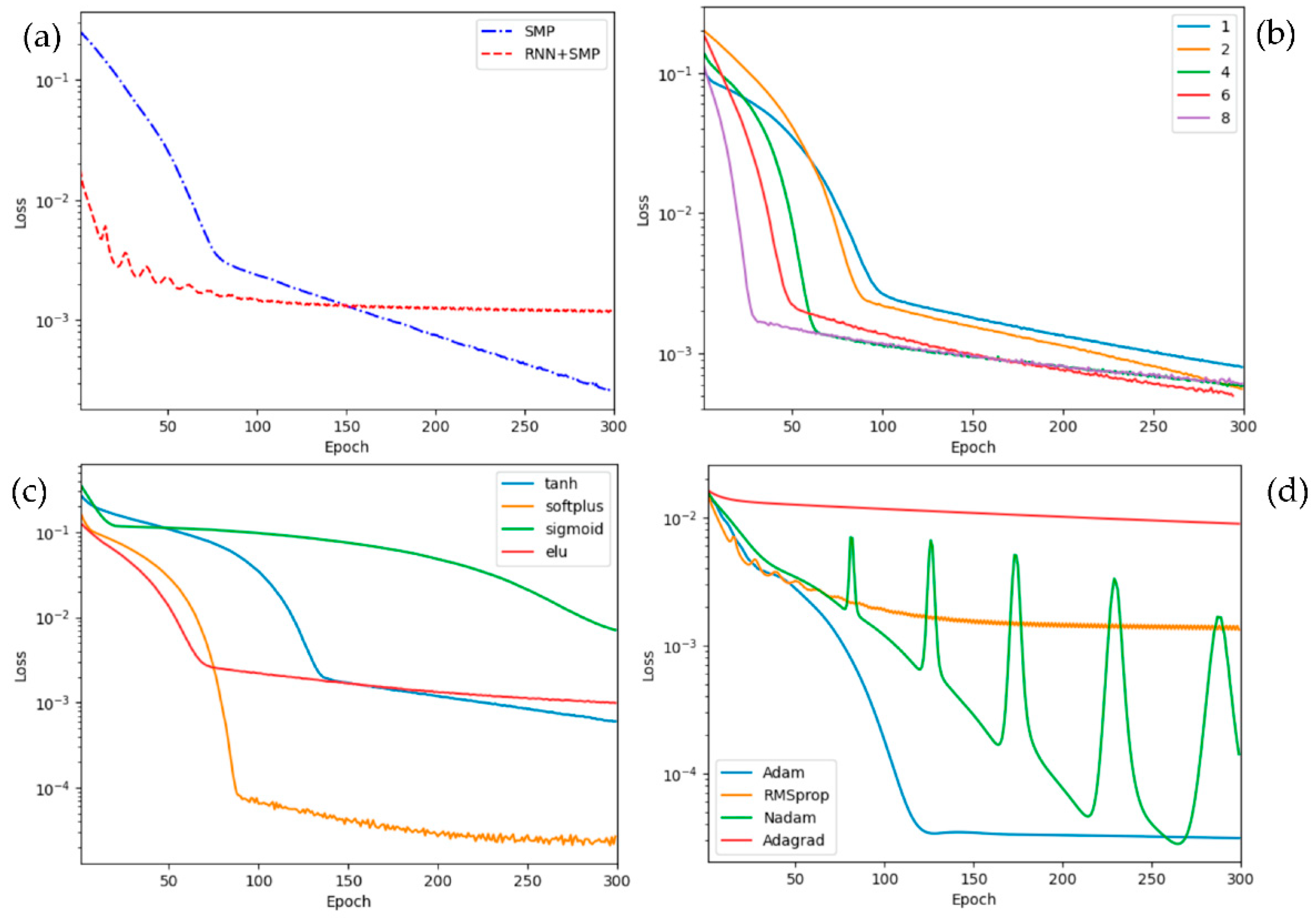
- Number of Epoch. To choose the optimal number of epochs, the loss of the forward simulation is performed by changing the number of epochs while keep the other settings intact in the default architecture. With the change of epoch, the epoch’s number contributing loss of SMP and SMP+RNN is illustrated in Figure 3 (a), where the former qualifies the fit of hidden variable and the latter is from the prediction of observations. It shows that the loss is decreasing dynamically during the first 80 epochs, but after that the loss is decreased slightly from to for MP while the loss of SMP+RNN starts to saturate and reach a plateau value of about . Therefore, greater than 80 is considered as the rule for determining optimal epoch’s number in the default architecture due to its stable loss of nearly .
- Layer in SMP. The computational complexity is concerned with the layer in SMP. Although decreasing layers are essential to reduce the complexity of SMP, the smaller number of SMP’s layer will affect the speed of convergence and the value of loss. According to the ‘for loop’ iteration method, different SMP of layer ranging from 1 to 8 is discussed to find an optimum value for obtaining a low complexity, fast converge, and small loss of SMP. As shown in Figure 3 (b), the increasing number of layers gives rise to the decreasing epoch value at which it starts to slowly converge, such as the100th epoch in the one layer compared with the 20th epoch in the 8 layers. Consequently, there is a trade-off between the computational time and the loss convergence in determining the favorite number of SMP layer, such as 2 or 3 layers.
- Activation function. Besides tanh, the other 3 activation functions softplus, sigmoid, and elu built in the TensorFlow library are used for the proposed architecture nodes, and their loss are compared in Figure 3 (c). The result shows that the widely used activation function ‘sigmoid’ is the worst choice, and moreover softplus-based architecture has the MSE loss of about 100 times smaller than that of the default architecture using ‘tanh’, which can be explained by the ability of softplus constraining the positive output for DR data. Hence, the activation function tanh in the default architecture nodes is replaced by softplus in the following.
- Optimizer. Four typical optimizers including Adam, RMSprop, Nadam, and Adagrad [9] are evaluated in the proposed method, and Figure 3 (d) illustrates the MSE loss varying with respect to the epoch for the four types of optimizers. From the aspect of minimum value of loss, Adam and Nadam reaches nearly while for the default RMSprop optimizer. However, the loss convergence of Adam is faster and more stable than that of Nadam especially after 50 epochs. Accordingly, the Adam or adaptive momentum optimizer is the best chose as the optimal hyperparameter tuning technique for the suggested neural network.
Figure 3.
Four factors affecting the loss of the proposed architecture: (a) Epochs of SMP configured with 2-layer dense and the SMP coded RNN or RNN+SMP; (b) Layers of SMP 1, 2, 4, 6, and 8 are considered; (c) Activation functions with tanh, softplus, sigmoid, and elu; and (d) Optimizers covering Adam, RMSprop, Nadam, and Adagrad.
Based on the above considerations, the default values of parameters choice in the architecture are updated to the optimal configurations, which consists of 3 layers of dense, softplus activation function, and Adam optimizer with the learning rate of . When compared to the results of the default architecture, seeing Figure 2 (b) and (c), the optimal architecture dramatically improves the performance of extracting predictions and hidden variables in Figure 4, where the loss value of the optimal of is lower than that of the default of about . Furthermore, no significant difference between the ideal and the trained predictions at the data tail is presented in Figure 4 (a). The optimal architecture seems a better fit for the hidden variable, such as a smaller difference between ‘initial setting-dR’ and ‘initial fitting-dR’ in Figure 4 (b), but this is not guaranteed for a good match between ‘trained dR’ and ‘ideal dR’ especially during the first second. In fact, the mismatch can be explained by the approximation error of the ideal reaction rate in Eq. (4), where the defect current of stretched exponential is well approximated by only when the time is large enough [1]. Therefore, the parameter estimation of optimal architecture is more accurate than the default architecture’s when it is employed in analyzing DR data.
3.3. Forward Calculation of Noisy Observations
During the DR measurement process, the observations of different samples can be corrupted by noise and recorded with different lengths. The noisy or truncated observations are assessed and contrasted to the ideal data in the above sections to validate the performance of the optimal architecture. The noisy observations, having SNR dB, stretched exponents , and numbers , is generated from the ideal data Eq. (1) by adding a Gaussian noise with mean 0 and SNR defined variance. Figure 5 demonstrates the influence of noise levels, stretched exponents, and numbers of observations on the accuracy of the optimal architecture, and the details are as the follows:
- SNR level. The noise has extraordinarily little influence on the predictions of the proposed architecture, especially for SNR level of greater than 20 dB, which is more evidently in SNR=20 dB of the about 5 times loss decrease, as compared to the SNR=10 dB, seeing Figure 5 (a). Additionally, Figure 5 (b) shows that the predictions agree well with the ideal observations when 400 noisy observations have and SNR=20 dB.
- Stretched exponent. The loss dependent on the stretched exponent is illustrated in Figure 5 (a). The loss value remains nearly constant at the same SNR level when the stretched exponent is a number between 0 and 1. For instance, the maximum deviation of the loss with respect to at SNR=40 dB is less than , and the minimum loss value at a bad SNR typically < 20 dB occurs at 0.6, which is the initial stretched exponent of defect current. Therefore, the forward method is not sensitive to the initial assumption of defect current for observations with a good SNR (>20 dB).
- Observation number. When the observation number N runs from 1600 down to 50, the loss value is lower than and stays nearly the same. Furthermore, a small observation number (N=5) can lead to the loss increase by 10 times, as compared to N=50. In short, the loss value reaches a stable convergence when N is greater than 50, seeing Figure 5 (c). In addition, there is no obvious influence upon the accuracy of predictions from noisy observations when the observation range is changed, such as from - 10 in Figure 5 (b) to -1 in Figure 5 (d).
In summary, the straightforward approach to implement the optimal architecture provides the forward calculation for DR analysis, where the empirical observations are subjected to noise interferences, unknown defect currents, and small training datasets, and has a small MSE loss of about even for less than 200 observations with a bad SNR level (< 20 dB) according to the classical simulation experiments.
4. Application for Extracting Physical Quantities
In this section, the four classical physical quantities: relaxation time spectrum, distribution of activation energies, number of defects visiting distinct sites, and dielectric loss, are extracted by the proposed forward method, and compared with that of the traditional inverse approach in the DR analysis.
4.1. Relaxation Time Spectrum
When SNR level runs from 10 dB to 60 dB, the determination of the relaxation time spectrum Eq. (3) is performed from the noisy DR data, seeing Figure 6 (a), where the ideal data generated from Eq. (1) has the exponent of 0.8 at the time constant of 1, and = 0.5 at . On the one hand, there is no obvious difference in the relaxation time spectrum of the same data with different SNR over 20 dB. For instance, the absolute error of relaxation time spectrum for SNR between 20 dB and 60 dB is less than 3% when exponent is 0.8; And moreover, the smaller the exponent, the more accurate extraction of the relaxation time spectrum. For example, the absolute error is only 0.9% at exponent of 0.5 while 3% at exponent of 0.8. On the other hand, when SNR is less than 10 dB, the absolute error is more than 5 times as large. Taking the 10 dB SNR data as an example, the absolute error reaches up to 4.9% for = 0.5 and 17.1% at = 0.8. However, the relaxation time spectrum extracted by the suggested method maintains the similar shapes of the ideal distribution even for a bad SNR typically less than 10 dB.
As stated in [6], the pending issue of the traditional method is the problem failing to yield an accurate parameter extraction from the DR data with SNR smaller than 40 dB. Contrasted with the classical poly fitting of the logarithmic transform of Eq. (1), the defect current-based RNN can obtain a precise estimation of the time spectrum or exponents at SNR over 10 dB. Therefore, the proposed method provides an alternative to the extraction of relaxation time spectrum from the noisy DR observations with a poor SNR.
4.2. Distribution of Activation Energies
Within the thermally activated Arrhenius relation for the time constant [10], the distribution of activation energies is linked to the relaxation time spectrum,
where denotes the activation energy, is the temperature, Boltzmann constant , H and L denote the subscript of parameters at the high and lower temperature, respectively, and .
After the extraction of the relaxation time spectrum and , the distribution of activation energies are determined by Eq. (9) and illustrated in Figure 6 (b), where observations are from the DR data of normally-off p-GaN HEMTs at 303 K and 423 K [2], and moreover SNR is tuned by the Gaussian noise as described in section 3.2.
The activation energy of the HEMT is in the ranges of 0.1-0.7 eV, and has a peak of 0.34 eV, which agrees well with the reports in [2]. In addition, the Gaussian-like distribution has a mean of 50.3 and standard of 32.1 for DR data of high SNR, such as 60 dB. With the decrease of SNR, the relative error of distribution is small such as 3.3% at 20 dB SNR relative to 60 dB SNR. Consequently, an accurate and robust determination of activation energy distribution is obtained from noisy observations when SNR is poor typically 10 dB or more.
4.3. Number of Defects Visiting Distinct Sites
As stated in Eq. (4), the defect current is described as the rate of a defect finding new sites, and thus leads to the estimation of the number of defects visiting distinct sites in time t, from the learned defect current,
When the defect current is learned, and by using the Laplace inverse of or . Figure 6 (c) gives the number of defects visiting distinct sites from the DR data with exponents of 0.1 to 0.9 with the step of 0.2, where the mean of is subtracted to highlight the dynamical behaviors of defects.
With the evolution of time t, increases, especially for the greater exponent, which means the defect diffusion becomes slower and highly dispersive for the lower exponent. This behavior of defect random walk agrees well with the findings in the above section that the wider the relaxation time spectrum or the distribution of activation energies is, the greater the exponent is. For Eq. (1) with , furthermore, it is considered as the result of classical diffusion-defect motion, which has for a linear chain [1]. Obviously, the theoretical at keeps consistent with the results of the suggested method, and the relative error is only 1.3%. Therefore, the DR data makes an implicit about the mean time between steps in the random walk with step and pausing-time distributions by the derived from the learned defect current.
4.4. Dielectric Loss
Considering the complex dielectric permittivity defined by Laplace transform of decay function [1], its imaginary part is called as the dielectric loss and can be derived by using the profile in Eq. (3),
Figure 6 (d) illustrates distributions of the dielectric loss at the exponents ranging from 0.1 to 0.9. As the exponent increases, the dielectric loss at the time constant increases, and its dependency of the angular frequency becomes more, obviously. The relationship between the dielectric loss and the angular frequency is consistent with the typical theoretical function for measured DR data, where the decay function has exponents of .
In fact, the exponent-dependent dielectric loss can be explained by the influence of defect diffusion. For smaller , the pausing time become longer, and speed of defect diffusion become slower, and thus leads to a litter combination rate between the lattices and defects or a lower dielectric loss. In return, the dielectric loss increases when the exponent parameter of DR data due to the faster defect diffusion in materials.
5. Conclusion
We have proposed a recurrent neural network methodology (RNN) encoded with the defect diffusion current for learning the physical quantities from the observations of dielectric relaxation (DR) in materials. The properties of dielectric relaxation including exponents and DR spectrum are estimated through the learned diffusion current. The suggested method with the optimal RNN architectures, consisting of 3 layers of dense, activation function softplus, and optimizer Adam with the learning rate of , is utilized to robustly extract the exponents of decay functions and the hidden defect currents for noisy DR observations of SNR of less than 20 dB. To validate the usefulness of the optimal physic-informed RNN, the physical quantities including the time spectrum, the distribution of activation energies, the number of defects visiting distinct sites, and dielectric loss are extracted, and compared with the available results. The proposed methodology leverages the priori defects diffusion-controlled chemical reaction to improve the robustness of the DR analysis due to the forward calculation instead of the inverse procedure in the traditional method, and thus casts a light on a powerful tool for investigating DR analysis in diverse dielectric materials.
Author Contributions
Conceptualization, X.L.; methodology, X.L. and J.Z.; software, X.L.; validation, X.L., Y.C. and J.Z.; formal analysis, J.Z.; investigation, X.L. and Y.C.; resources, X.L.; data curation, J.Z.; writing—original draft preparation, X.L.; writing—review and editing, J.Z., and Y.C.; visualization, X.L. All authors have read and agreed to the published version of the manuscript.
Funding
Manuscript received Dec. 1, 2022. This work was supported in part by the Natural Science Foundation of Chongqing under Grant cstc2019jcyj- msxmX0490, the Science and Technology Research Program of Chongqing Municipal Education Commission under Grant KJZD–K202000504, and the Chongqing Education Planning Project under Grant 202-GX –277.
Informed Consent Statement
Not applicable.
Conflicts of Interest
The authors declare no conflict of interest.
References
- Shlesinger, M.F.; Montroll, E.W. On the Williams—Watts function of dielectric relaxation. Proc. Natl. Acad. Sci. 1984, 81, 1280–1283. [Google Scholar] [CrossRef] [PubMed]
- Modolo, N.; De Santi, C.; Minetto, A.; Sayadi, L.; Prechtl, G.; Meneghesso, G.; Zanoni, E.; Meneghini, M. Trap-state mapping to model GaN transistors dynamic performance. Sci. Rep. 2022, 12, 1755. [Google Scholar] [CrossRef]
- Stetsovych, V.; Feigl, S.; Vranik, R.; Wit, B.; Rauls, E.; Nejedlý, J.; Šámal, M.; Starý, I.; Müllegger, S. Towards dielectric relaxation at a single molecule scale. Sci. Rep. 2022, 12, 2865. [Google Scholar] [CrossRef] [PubMed]
- Koh, S.-G.; Shima, H.; Naitoh, Y.; Akinaga, H.; Kinoshita, K. Reservoir computing with dielectric relaxation at an electrode–ionic liquid interface. Sci. Rep. 2022, 12, 6958. [Google Scholar] [CrossRef] [PubMed]
- Pereyra, V.; Scherer, G. Exponential Data Fitting and Its Applications. Bentham Science Publishers, Sharjah, 2018.
- Choi, H.; Vinograd, I.; Chaffey, C.; Curro, N. Inverse Laplace transformation analysis of stretched exponential relaxation. J. Magn. Reson. 2021, 331, 107050. [Google Scholar] [CrossRef] [PubMed]
- The numerical integration of the first order differential equation through the Euler method given that the time history of far-field stresses. Available at: https://github.com/PML-UCF/pinn_ code_tutorial.
- Karniadakis, G.E.; Kevrekidis, I.G.; Lu, L.; Perdikaris, P.; Wang, S.; Yang, L. Physics-informed machine learning. Nat. Rev. Phys. 2021, 3, 422–440. [Google Scholar] [CrossRef]
- Optimizers in Tensorflow. Available at: https://www.geeksforgeeks.org/optimizers-in-tensorflow/.
- Pobegen, G.; Aichinger, T.; Nelhiebel, M.; Grasser, T. Understanding temperature acceleration for NBTI. In Proceedings of the 2011 IEEE International Electron Devices Meeting (IEDM), Washington, DC, USA, 5–7 December 2011. [Google Scholar] [CrossRef]
- Ward, I. Polymer motion in dense systems: Springer proceedings in physics 29. Polymer 1989, 30, 373–373. [Google Scholar] [CrossRef]
- Milovanov, A.; Rasmussen, J.; Rypdal, K. Stretched-exponential decay functions from a self-consistent model of dielectric relaxation. Phys. Lett. A 2008, 372, 2148–2154. [Google Scholar] [CrossRef]
- Alvarez, F.; Alegra, A.; Colmenero, J. Relationship between the time-domain Kohlrausch-Williams-Watts and frequency-domain Havriliak-Negami relaxation functions. Phys. Rev. B 1991, 44, 7306–7312. [Google Scholar] [CrossRef]
- Pang, Y.; Sun, M.; Jiang, X.; Li, X. Convolution in Convolution for Network in Network. IEEE Trans. Neural Networks Learn. Syst. 2017, 29, 1587–1597. [Google Scholar] [CrossRef]
- Ananthakrishnan, A.; Allen, M.G. All-Passive Hardware Implementation of Multilayer Perceptron Classifiers. IEEE Trans. Neural Networks Learn. Syst. 2020, 32, 4086–4095. [Google Scholar] [CrossRef] [PubMed]
Figure 1.
Framework of defect diffusion-informed recurrent neural network (RNN) with outputs of full sequences and a cell of shallow multilayer perceptron (SMP) for analyzing DR.
Figure 1.
Framework of defect diffusion-informed recurrent neural network (RNN) with outputs of full sequences and a cell of shallow multilayer perceptron (SMP) for analyzing DR.
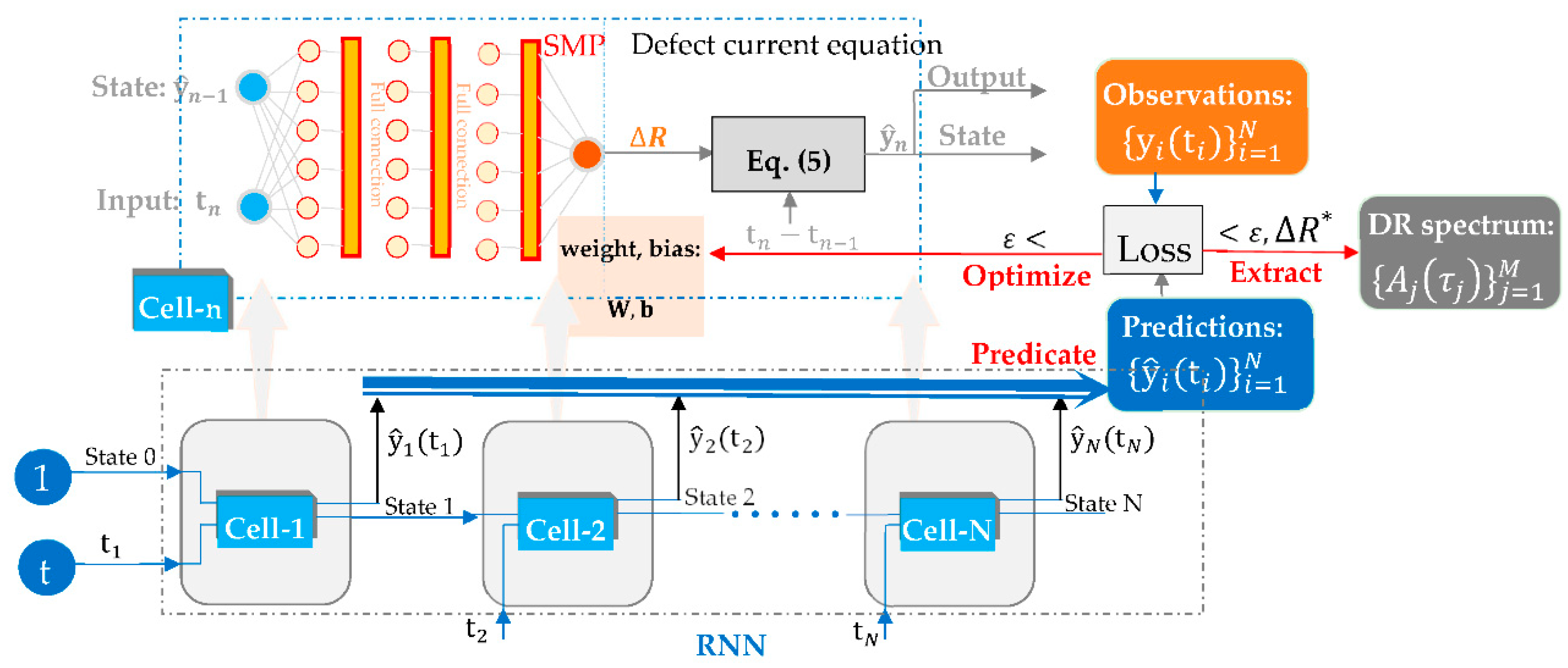
Figure 2.
Illustration of implementing the proposed method for the analysis of stretched exponential functions at τ=1. (a) Observations, defect current, and hidden variable ∆R from the classical equations at α=0.7; (b) The expressivity and learnability of SMP embedded in RNN for ∆R at three steps including the setting and the fitting at the initiation, the trained by observations from Eq. (1) at α=0.7; (c) Comparisons of predictions before and after training for an arbitrary given condition; (d) Relaxation time spectrums extracted when α=0.5,0.7,0.98.
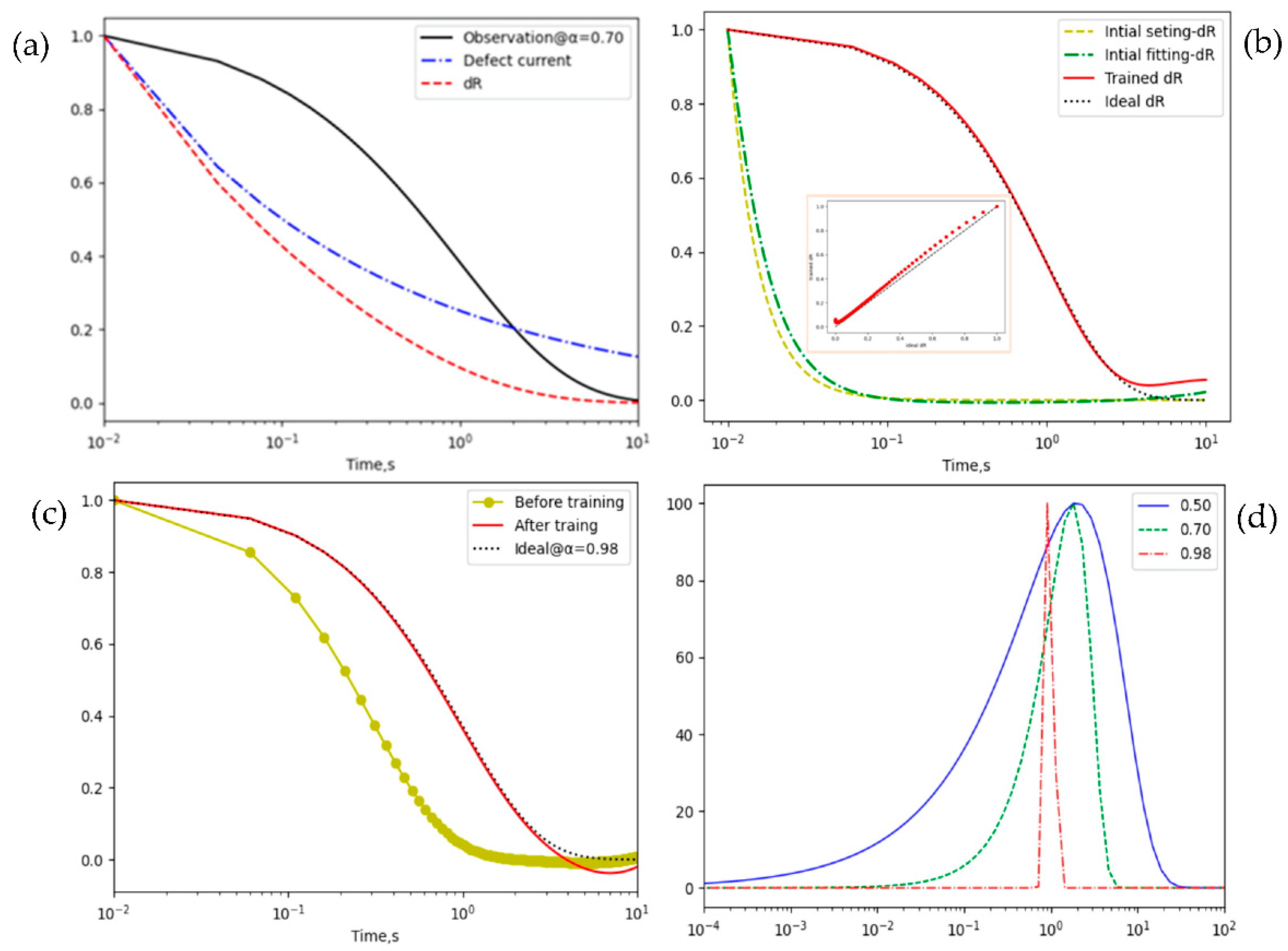
Figure 4.
The reconstructed observations and hidden variables by using the optimal architecture according to the observational data for plotting Figure 2 (b) and (c), which has a loss value of and consists of 3 layers of dense, softplus activation function, and Adam optimizer with the learning rate of .
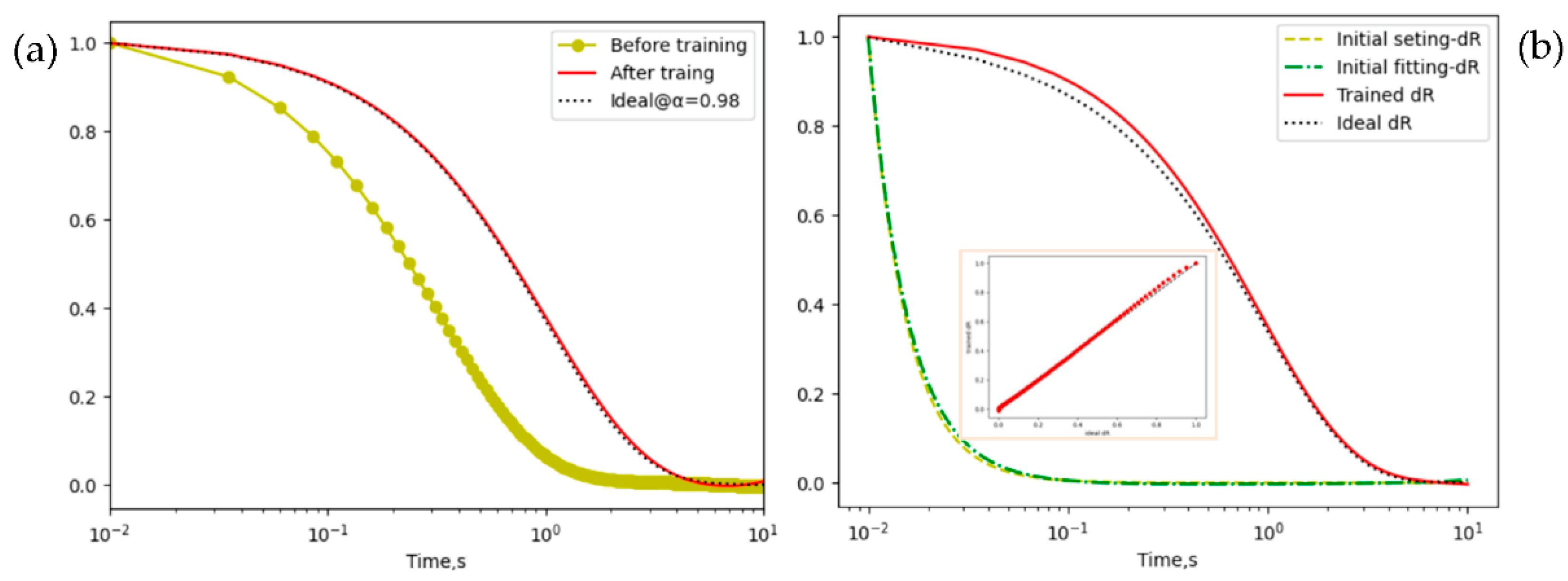
Figure 5.
Influence of noise level, stretched exponent, and number of observations on the accuracy of optimal architecture. (a) Relationship between the loss and SNR and exponents; (b) The reconstructed from the noisy data with SNR=20 dB and exponent of 0.9 at the time range from to 10; (c) Curve of the loss and data length N; (d) Predictions from the 20 dB SNR, 0.8 exponential data at the time range from to 1.
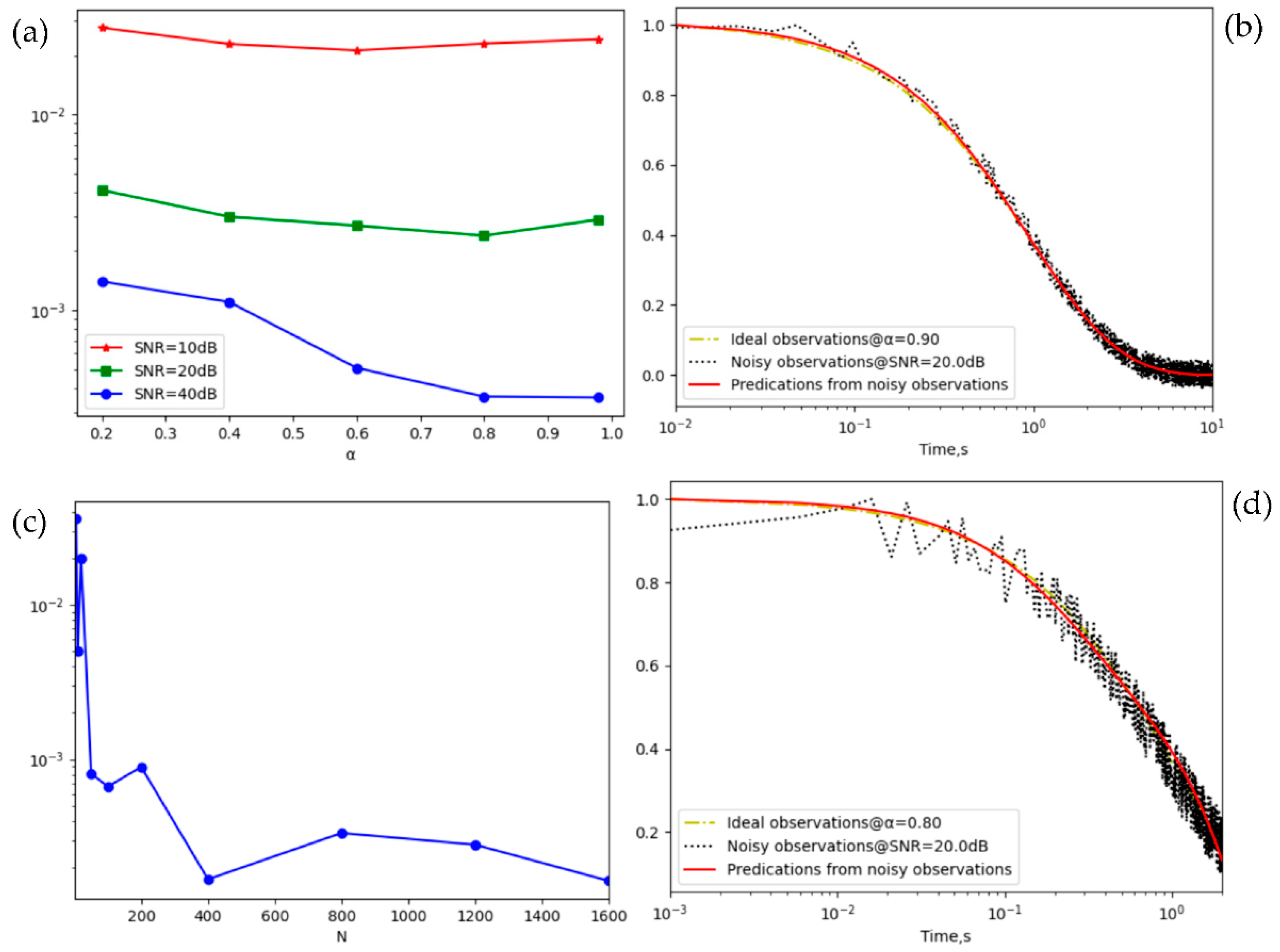
Figure 6.
Illustrations of physical quantities extracted by the defect current-based RNN: (a) Relaxation time spectrum of the noisy data with = 0.5 and ,= 0.8 and at SNR of 10, 20, 40, and 60 dB, respectively; (b) Distribution of activation energies of HEMTs [2] from observations with SNR of 20 dB and 60 dB; (c) Number of defects visiting distinct sites from the data with exponents ranging from 0.1 to 0.9 with the step of 0.2, where the mean of is subtracted and the theoretical value at is compared; (d) Dependency of dielectric loss on angular frequency ranging from to and exponents within the range of 0.1-0.9.
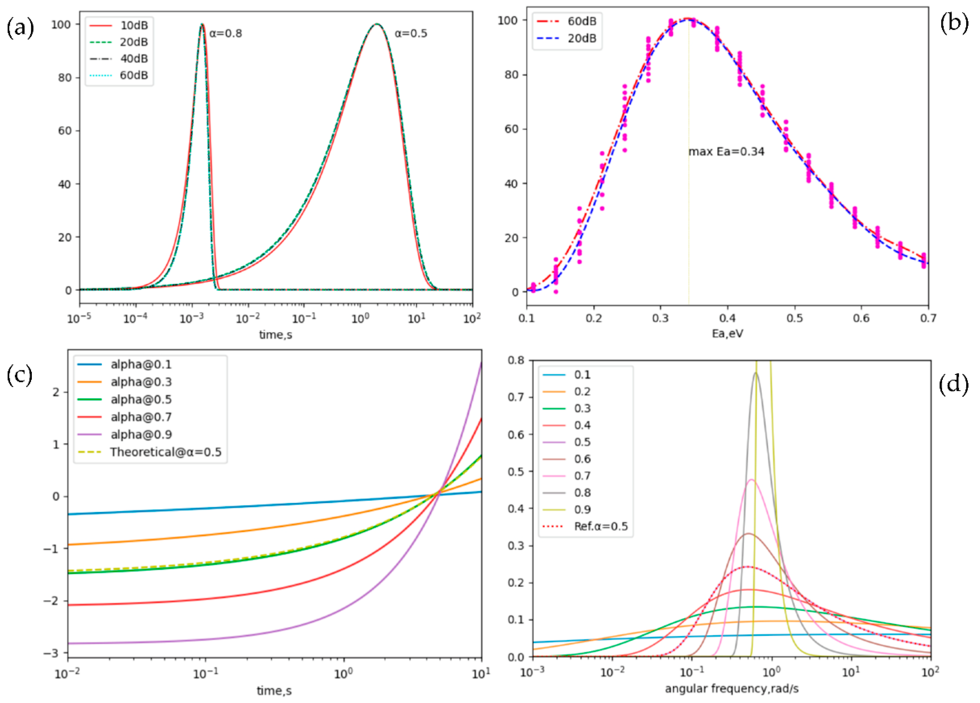

Table 1.
Pseudocode of defect current-informed RNN.
| Step | Function | Main Python Code | Comment |
|---|---|---|---|
| 1 | Import libraries or modules | from scipy.special import gamma from tensorflow.keras import Sequential from tensorflow.keras.layers import RNN, Dense, Layer |
-Preparation. |
| 2 | Create model for SMP | dRlayer = Sequential() dRlayer.add(Dense(5, activation='tanh')) |
-SMP with numbers of layer 5, and the form of activation ‘tanh’. |
| 3 | Initiate weights and biases of SMP | t=np.linspace(1e-2,1e1,400) y_range=np.logspace(-6,0,400) dR0 =dfct_current(t,0.7)* y_range dRlayer.compile(loss='mse', optimizer=RMSprop(1e-3) dRlayer.fit([t,y_range], dR0, epochs=200) |
- 400 observations ranging from 0.01 to 10 s, and having the amplitude range from 10-6 to 1. -dR0 is the initial using the dfct_current function or in Eq. (4). -Configure optimization with the MSE loss function, optimizer RMSprop, and training data. |
| 4 | Generate a cell instance | class Cell_n(Layer): def call(self, inputs, states): dy_n= - self.C * self.dRlayer([inputs, states[0]]) yn=dy_n+states[0] return yn, [yn] |
-Define a layer to realize the Cell-n in Fig. 1, where the call function oversees the SMP forward calculation or self.dRlayer and the prediction of Eq. (5). |
| 5 | Construct RNN | DCIRNN = RNN(cell= Cell_n,return_sequences=True) model = Sequential() model.add(DCIRNN) |
-Embed the Cell_n into RNN with the return sequence for all predictions and generate the model. |
| 6 | Forward prediction | model.compile(loss='mse', optimizer=RMSprop(1e-2)) model.fit(t, observs, epochs=20, steps_per_epoch=1) yPred = model.predict_on_batch(t)[:,:] |
-Configure the loss function and optimizer. -Fit the experimental observations. -Obtain the predictions |
| 7 | Extract DR spectrum | Ait= Pbltf(1/t,alpha,tao0)*np.abs(np.diff(1/t)) | - Pbltf is the asymptotic in Eq. (3). |
Disclaimer/Publisher’s Note: The statements, opinions and data contained in all publications are solely those of the individual author(s) and contributor(s) and not of MDPI and/or the editor(s). MDPI and/or the editor(s) disclaim responsibility for any injury to people or property resulting from any ideas, methods, instructions or products referred to in the content. |
© 2025 by the authors. Licensee MDPI, Basel, Switzerland. This article is an open access article distributed under the terms and conditions of the Creative Commons Attribution (CC BY) license (http://creativecommons.org/licenses/by/4.0/).
Copyright: This open access article is published under a Creative Commons CC BY 4.0 license, which permit the free download, distribution, and reuse, provided that the author and preprint are cited in any reuse.


