
Submitted:
26 March 2025
Posted:
27 March 2025
You are already at the latest version
Abstract
(1) Background: Although the field of natural product (NP) drug discovery has been extensively developed, there are still several bottlenecks hindering the development of drugs from NPs. The PD-1/PD-L1 immune checkpoint axis plays a crucial role in immune response regulation. Therefore, drugs targeting this axis can disrupt the interaction and enable immune cells to continue setting up a response against the cancer cells; (2) Methods: We have explored the immuno-oncological activity of NPs targeting the PD-1/PD-L1 immune checkpoint by estimating the half maximal inhibitory concentration (IC50) through molecular docking scores and predicting it using machine learning (ML) models. The LightGBM (Light Gradient Boosted Machine) a tree-based ML technique emerged as the most effective approach and was used for building the quantitative structure–activity relationship (QSAR) regression models; (4) Conclusions: The model incorporating 570 spectral descriptors from NMR SPINUS was selected for optimization process, and this approach yielded results for the training set with a MAE of 0.22, RMSE of 0.30 and R-squared of 0.86. The strategy used here of estimating the IC50 from docking scores and predicting it through ML models appears to be a promising approach for pure compounds. Nevertheless, further optimization is indicated, particularly through the simulation of spectra of mixtures by combining the spectra of individual compounds.
Keywords:
natural products (nps)
; immuno-oncology
; pd-1/pd-l1 immune checkpoint
; machine learning (ml) techniques
; molecular docking
; nuclear magnetic resonance (nmr)
; quantitative structure–activity relationship (qsar) models
; virtual screening
1. Introduction
The statistical analysis of new drug approvals by the Food and Drug Administration (FDA) from 2011 to 2020 reveals a significant upward trend in the annual approval rate of new molecular entities (NMEs) [1]. During this period, the 10-year average reached 31.4 NMEs per year, a notable increase compared to the previous decade (2001–2010), which averaged 18.4 NMEs annually [1,2,3,4,5]. In contrast, natural products (NPs) and NP derivatives showed steady approval rates over time, with a 10-year average of 4.2 and 3.8 drugs per year for the decades 2001–2010 and 2011–2020, respectively [1,2,3,4,5]. Interestingly, the peak approval for NP and NP derivatives occurred in 1996, with 12 drugs approved, and the 1990s were also the most prolific for computer-aided drug design (CADD)-driven drugs, with eight approvals [2]. Additionally, over half of all approvals for marine natural products (MNPs) and MNP derivatives were in the 21st century, with eight of the eleven approved drugs occurring after 2000 [1,2,3,4,5]. New strategies are essential to address the perceived disadvantages of NPs compared to synthetic drugs, including challenges in accessibility and supply that delayed MNP research until the 1980s [1,2,6,7]. For example, the development of marine-derived drugs is a lengthy and costly process, taking between 17 years (e.g., trabectedin, Yondelis®) and 24 years (e.g., halichondrin, Halaven®; dolastatin, ADCetris®), with an average of 23 years from the initial discovery of an MNP to its market approval [6]. To mitigate these challenges, CADD approaches can support decisions on in vivo and in vitro testing of isolated NPs and extracts, facilitate the design of bioactive NP derivatives, and enable virtual screening of databases containing known or proposed NPs. The COlleCtion of Open NatUral producTs (COCONUT), an open-access database of NPs launched in 2021 at https://coconut.naturalproducts.net [8], is one of the largest resources available for NP annotation [8,9]. The database contains structures of over 695,000 unique NPs, including 82,220 molecules without stereocenters, 539,350 molecules with defined stereochemistry, and 73,563 molecules with stereocenters but undefined absolute stereochemistry. [9]. Currently, COCONUT encompasses a vast collection of NPs derived from 63 data sources, including PubChem NPs (with 2,020 entries), ChEBI NPs (12,935 entries), ZINC NP (76,616 entries), CMNPD: A Comprehensive MNPs Database (26,981 entries), and the Latin American NP Database (LANaPDB) (12,935 entries) [9]. COCONUT provides valuable features, including predicted molecular properties, molecular descriptors, information on names and synonyms, species and organism parts where the NP has been identified, geographic details about the collection site of the sample, and literature references supporting all this information [9]. The complete set of structures is available for download in SDF, CSV, and database dump formats, enabling integration with other structural feature-based databases for dereplication purposes [9].
Understanding where biologically relevant compounds reside within the chemical structural space—and how these two realms, chemical and biological, intersect—is crucial for unlocking new insights and driving innovation in the exploration of NPs. The regions of chemical space surrounding NPs are widely recognized as highly promising for the development of new drug leads, as demonstrated in a comprehensive analysis spanning the period from 1981 to September 2019. NP scaffolds—including unaltered NPs, NP derivatives, NP mimetics, and structures containing an NP pharmacophore—account for 45% of all approved small-molecule drugs [10]. A structural classification analysis of NPs conducted by Waldmann and colleagues [11] revealed that over half of all NPs possess an optimal size (a van der Waals volume between 300 and 800 ų), making them well-suited as starting points for hit-to-lead discovery. Similarly, Pereira et al. [12] reported a strong correlation between active compounds and three- or four-ring structures with a van der Waals volume within the same range in a distinct PubChem subset. To further enhance the exploration of NP chemical space, Ertl et al. [13] developed an NP-likeness score, which quantifies the similarity of a molecule to the structural features of NPs. This metric has been integrated into the COCONUT database, providing researchers with a valuable tool for drug discovery and development [9]. Recently, two complementary studies have shed light on the distinctions between terrestrial natural products (TNPs) and marine natural products (MNPs) [14,15]. Shang et al. [14] utilized chemoinformatics methods to analyze these differences, while Pereira [15] applied ML modeling to predict the terrestrial or marine origin of NPs. Both studies highlighted a trend where MNPs tend to contain more halogens (particularly bromine) and fewer oxygen-containing groups compared to TNPs [14,15]. However, the studies reached different conclusions regarding ring size. Shang et al. [14] reported that larger rings, particularly those with 8 to 10 members, were more prevalent in MNPs. In contrast, Pereira [15] found that 5-membered rings were more significant in distinguishing MNPs. Despite these discrepancies, Pereira [15] observed a clear separation between the chemical spaces occupied by MNPs and TNPs when employing ML techniques, underscoring the distinct nature of these two groups of NPs.
The clinical translation of immune checkpoint inhibitors (ICIs), which modulate T cell activation, was the most significant advancement in cancer treatment over the past decade [16]. Currently, eight PD-1/PD-L1 ICIs have been approved [16]. While all approved ICIs are monoclonal antibodies (mAbs), they present challenges such as poor oral bioavailability, prolonged tissue retention, low membrane permeability, and high costs. As a result, research has shifted toward developing small molecule inhibitors to address these limitations [16]. Few studies have explored CADD for PD-1/PD-L1 inhibition [17], with most relying on Structure-Activity Relationship (SAR) analysis and PD-L1 docking, mainly based on Bristol-Myers Squibb (BMS) compounds [18,19,20,21,22,23]. Our group recently reported an integrated CADD approach combining QSAR modeling, drug repurposing, and molecular docking, offering a novel strategy for PD-1/PD-L1 inhibition [24]. In the same study, sonidegib, an anticancer drug with a biphenyl system, was identified as a potential hit and later validated for in vitro PD-1/PD-L1 binding modulation using ELISA and flow cytometry [24].
The ability to predict biological activity through inexpensive, rapid and automated testing of extracts is a transformative technology that enables the selection of promising extracts prior to isolation and structure elucidation of compounds. Biological activity is a consequence of molecular structure, and the latter is reflected in NMR spectra. For several classes of compounds, ML techniques have been used to automatically extract structural features [25] and also to predict physical/chemical properties [26] and biological activities [27] from NMR spectra - Quantitative Spectrometric Data-Activity Relationships (QSDAR) - and 13C NMR spectra have been found to be necessary in addition to 1H NMR. Although their predictive power is generally lower than that of QSAR, QSDAR has the enormous advantage of not requiring the structure of the compound (only its spectra). Latino & Aires-Sousa showed that ML algorithms such as Kohonen Self-Organizing Maps (SOMs), Random Forests (RFs) and counter-propagation neural networks (CPNN) can classify photochemical and metabolic reactions from the difference between the 1H NMR spectrum of the products and the reactants [28,29]. Recently, the use of QSDAR models to discover new inhibitors against the human colon carcinoma HCT116 cell line [30] and methicillin-resistant Staphylococcus aureus (MRSA) infection [31] has also been reported by Pereira and co-workers. The QSDAR classification models were built using the experimental 1H and 13C NMR spectra obtained from 50 crude extracts, 55 fractions and 50 pure compounds from actinobacteria isolated from marine sediments collected off the Madeira Archipelago [32].
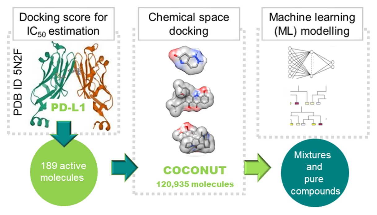
The present study was undertaken to investigate the immuno-oncological activity of NPs that target the PD-1/PD-L1 immune checkpoint. To this end, the IC50 was estimated on the basis of molecular docking scores and predicted using ML models. The dataset was extracted from the COCONUT database and comprised 120,935 molecules with a HeavyAtomMolWt (the average molecular weight of the molecule, ignoring hydrogens) of less than 500 Da. All 120,935 NPs in the dataset were subjected to molecular docking against the PD-L1 receptor (PDB ID 5N2F) in order to predict the conformations and scores associated with the docking process. The QSDAR models for pure compounds were developed using two distinct approaches to spectral data calculation. The first approach employed a graph neural networks (GNN) model to predict NMR chemical shifts - NMR GNN. The second approach utilized the SPINUS program (https://neural.dq.fct.unl.pt/spinus/) to predict both 1H NMR chemical shifts and coupling constants - NMR SPINUS. The support vector machine (SVM), convolutional neural network (CNN), RF, and light gradient boosted machine (LightGBM) were the four machine learning techniques explored. The objective was to predict PD-1/PD-L1 inhibition, with the performance of the models assessed through internal and external validation. The tree-based ML technique, LightGBM, was identified as the most effective approach and was therefore employed for the construction of the QSDAR regression models. The model comprising 570 spectral descriptors derived from SPINUS exhibited the most favorable performance for the training set, with a mean absolute error (MAE) of 0.22, root mean square error (RMSE) of 0.30 and R-squared value of 0.86. Furthermore, the performance of these QSDAR models was benchmarked against that of conventional QSAR models utilizing molecular, fingerprint, and quantum descriptors. The strategy of estimating the half maximal inhibitory concentration (IC50) from docking scores and predicting it through ML models appears to be a promising approach for pure compounds. Nevertheless, further optimization is possible, particularly through the simulation of mixtures by combining the spectra of individual compounds.
2. Results and Discussion
2.1. Docking score for the estimation of IC50 values
The potential of utilizing the calculated free binding energies (ΔGB) by molecular docking with AutoDock Vina (version 1.2.3) was investigated as an output of the QSDAR model. A total of 189 molecules with a HeavyAtomMolWt of less than 500 Da, as reported in the literature as active against PD-1/PD-L1, were subjected to molecular docking with PD-L1. The correlation between pIC50 and ΔGB for these molecules was subsequently analyzed (Figure 1).
As can be seen in Figure 1, there is a correlation between the docking scores and the experimental pIC50 values. Furthermore, we have complete control over the calculated values, i.e. all molecules are calculated using the same procedure. This is something we cannot guarantee when using experimental values from different sources. Therefore, all 120,935 NPs in the dataset were docked to the PD-L1 receptor (PDB ID 5N2F) to predict docking conformations and scores. The interactions of the best docked unclassified NP, CNP0035993, plant NP, CNP0386002, fungal NP, CNP0133095, and MNP, CNP0144730, with PD-L1 were analyzed and compared to the positive control, BMS-200 (Figure 2).
Figure 2 illustrates the chemical structure of one of the predicted NPs with the lowest ΔGB (A). The structure features the biphenyl moiety, highlighted in blue, along with the predicted binding pose. It can be observed that there are different binding poses for the two NPs above (A and B) in comparison to the positive control (BMS-200, E), particularly the lack of interaction with Tyr56 of chain A. The two NPs from fungal and marine sources depicted in the image (C and D) were found to exhibit binding poses that were similar to those of the positive control. The experimental IC50 value displayed in Figure 2, 80 nM, for BMS-200 (E) can be compared with the value of IC50 estimated by molecular docking, which was found to be 52.2 nM.
The SMILES strings of the 189 molecules comprising the active data set (as reported in the literature as active against PD-1/PD-L1) are available as Supplementary Material, Table S1, along with the corresponding experimental activities (IC50) and estimated ΔGB.
2.2. QSDAR Regression Modelling
2.2.1. Dataset
The dataset was extracted from the COCONUT database and consists of more than 120,000 molecules with a HeavyAtomMolWt of less than 500 Da, which were subjected to molecular docking against the PD-L1 protein and spectral data calculations.
The dataset displays the following distribution: the majority remains unclassified, with 14% originating from plant-derived natural products, 3% from marine sources, 1% from bacteria, and 4% from fungi, Figure 3.
The entire data set, comprising 120,935 NPs, was randomly partitioned into a training set of 119,733 molecules and a test set of 1,202 molecules.
These sets were employed for the development (training set) and external validation (test set) of the QSDAR regression models. It is generally accepted that a given compound exhibits considerable inhibitory activity when the IC50 is less than or equal to 10 µM. This value is typically employed to differentiate between active and inactive compounds. Table 1 presents an analysis of the data set, which has been divided into training and test sets. These have been fractionated by active and inactive category, and the drug-likeness characteristics (e.g. HeavyAtomMolWt, MolLogP) and the NP-likeness score has also been considered.
As evidenced by the analysis in Table 1, the test set appears to be a reliable representation of the training set. This is evident from the comparable distribution of active and inactive NPs between the two sets, as well as from the consistency in drug-likeness and NP-likeness parameters. A significant proportion of NPs, exceeding 84%, in both the training set and the test set adhere to two of Ghose's rules [34], thereby substantiating the high degree of drug-likeness inherent to the dataset derived from the COCONUT database. Ertl et al. [13] developed the NP-likeness score and mapped this score onto the various chemical spaces. It was observed that for an NP-likeness between -1 and 1, there seems to be a higher percentage of drugs. Thus, for our data set, the percentage of NPs with the highest similarity with drugs is greater than or equal to 43%.
2.2.2. Spectral Data
NMR GNN: The NMR chemical shifts were predicted by a graph neural networks (GNN) model developed by Yang et al. in Python [35]. The chemical shifts and type (H, C, N, O, etc.) were encoded by a fixed-length numerical code of 250 spectral descriptors.
1H NMR SPINUS (Structure-based Predictions In NUclear magnetic resonance Spectroscopy): 1H NMR chemical shifts and coupling constants were predicted by ensembles of feed-forward neural networks (FFNN) and were incorporated into Associative Neural Networks (ASNN), https://neural.dq.fct.unl.pt/spinus/, [36,37]. A fixed length numerical code of 570 spectral descriptors encoded the discrete values of the 1H chemical shifts and coupling constants.
2.2.3. QSDAR Model Development
The RF ML technique was employed for the construction of QSDAR models to predict PD-1/PD-L1 inhibition based on two distinct NMR spectral descriptors (e.g. SPINUS, GNN). The efficacy of the models was successfully evaluated through internal validation (OOB estimation for the training set), as illustrated in Table 2.
The model comprising 820 spectral descriptors derived from NMR GNN and SPINUS exhibited the most favorable performance for the training set, with a MAE of 0.20, RMSE of 0.26 and an R2 of 0.91. Despite the QSDAR model with the NMR SPINUS descriptors demonstrating a reduced predictive capacity in comparison to the NMR SPINUS and GNN model for the training set, with an MAE of 0.23, an RMSE of 0.30 and an R2 of 0.88, it is selected for the subsequent optimization process. This is primarily due to its capacity to more accurately reproduce the experimental NMR spectrum, whilst also utilizing the prediction of 1H NMR data. Subsequently, this model was further optimized through descriptor selection, based on the importance assigned by the RF model using the 50, 100, 150 or 200 most important descriptors, as illustrated in Table 3.
The selection of the 150 most important descriptors from the NMR SPINUS spectral descriptor set, used to build the model with the RF, enabled the training of much smaller RF models with equivalent prediction accuracies (R2 = 0.88 and MAE = 0.22) to those achieved by models trained with the complete set of descriptors for the training set. A comparison of four ML techniques using RF, LightGBM, SVM and CNN for building the PD-L1 models with the 150 most important spectral descriptors selected by the RF descriptor importance is shown in Table 4.
It is clear that the best QSDAR model was achieved using the LightGBM algorithm. This is evidenced by the lower MAE and RMSE obtained for the training set in cross-validation estimation (see Table 4). Figure 4 and Figure 5 show the predicted versus calculated pIC50 for the ligand-PD-L1 complex in the training and test sets, respectively.
2.3. Benchmarking with QSAR Using Molecular, Fingerprint, and Quantum Descriptors
The performance of QSDAR models constructed using spectral data that were reported in Section 2.2 was evaluated in comparison with more conventional QSAR models using fingerprints (FPs), 2D and 3D molecular descriptors, encompassing three distinct types of FPs with varying sizes (166 MACCS; 1024 Morgan, circular fingerprints and 2048 RDKit). A total of 242 1D&2D molecular descriptors were employed, encompassing electronic, topological, and constitutional descriptors, as well as three types of 3D molecular descriptors: Autocorr3D (80 descriptors), Getaway (271 descriptors), and Radial Distribution Function, RDF (210 descriptors). The RDKit software, which is written in both C++ and Python, was employed for the calculation of molecular descriptors and FPs [38]. Fast estimation of Density functional theory (DFT) properties, previously developed by ML techniques in our group for molecular orbital energies [39] and dipole moment [40], enable to include five quantum descriptors such as the energy of the highest occupied molecular orbital (εHOMO), the lowest unoccupied molecular orbital (εLUMO), HOMO−LUMO gap, dipole moment (DM) calculated using empirical point natural bond orbital (NBO) charges [41] and DFT-DM.The tree-based ML technique, LightGBM, was identified as the most effective approach in the QSDAR regression models and was also used to build the QSAR models. The models' performance was successfully evaluated through internal validation (10-fold cross-validation for the training set), as depicted in Table 5.
The performance of the 3D descriptors in modelling activity against PD-L1 was noteworthy. For each type of 3D descriptor, the predictions achieved an R2 of at least 0.99 and an MAE of less than 0.04. We believe that this impressive capacity is attributable to the utilisation of a conformation for each NP that has been optimised through alignment with the conformation obtained through molecular docking against the PD-L1 receptor (PDB ID 5N2F), as detailed in the Methods section (3.1. Datasets: Training and test sets). The most appropriate set of FPs and descriptors, comprising 1D&2D, along with all 3D descriptors, were selected for further investigation (see Table 6).
2.4. Applicability Domain of PD-L1 QSDAR Model
The applicability domain of a QSAR model highlights the part of a chemical space containing the compounds for which the model is able to provide reliable predictions. A Tanimoto Coefficient (TC) matrix approach was used to define the applicability domain of the PD-L1 QSDAR model based on the similarity between a molecule in an external data set, 1,202 molecules of the test set, and all 119,733 molecules in the training set. The Tanimoto coefficient of similarity was calculated using an RDKit script [38]. A TC is a similarity value between 0 and 1 for a given pair of molecules. The closer two molecular structures are to one another, the higher the TC value. By analysing the TC matrix and the MAE values obtained with the best QSDAR model for the test set, we were able to define a threshold based on the average TC value obtained by a given molecule in the test set and all the molecules in the training set. Accordingly, for a given molecule that the model has not previously encountered, the predicted values should be considered reliable if the molecule exhibits an average TC value exceeding or equally to 0.20 in comparison to all the molecule of the training set. Upon applying this threshold to the test set, 176 molecules are excluded. Considering the optimal QSDAR model, an MAE of 0.38 is obtained for the 176 molecules located outside the model's applicability domain, compared to an MAE of 0.37 for the 1026 molecules within the applicability domain (Figure 6). Available as Supplementary Information, Table S3, are the SMILES strings of 176 molecules outside the applicability domain of the model from the test set and the absolute error obtained by the best QSDAR model.
2.5. Analysis the Test Set Predictions with PD-L1 QSDAR Model
With regard to the predictions for the test set, particular attention is given to the top-performing predictions (i.e. those obtained with MAE < 0.3752/3) and the outliers (i.e. those obtained with MAE > 0.3752*3). Twenty-three percent of the molecules in the test set are very well predicted, with an MAE below 0.13. Figure 7 presents two examples, including their structures and binding poses to the PD-L1 protein. It is observed that the well-predicted active molecule exhibits a binding pose similar to the positive control. The small bicyclic heterocyclic compound is accurately predicted to be inactive and adopts a different binding pose. On the other hand, molecules with an MAE greater than 1.13 are considered outliers, representing only 2.5% of the test set. Their binding poses are also shown in Figure 7. With the exception of the NP, CNP0000488, all three NPs highlighted in Figure 7 belong to the model's applicability domain with an average TC greater than or equal to 0.20.
2.6. Virtual Screening
As stated in the introduction, the two anticancer drugs, sonidegib and lapatinib, were identified as potential inhibitors of PD-L1 by our group using an integrated CADD approach in a previous study [24]. Consequently, in order to validate the QSDAR model developed in the present study, it can be employed in the virtual screening procedure of the two anticancer drugs proposed in our previous study [24] and the positive control (BMS-200, Figure 2 - E). The most suitable model identified for the virtual screening procedure was the lightGBM regression model, which employed the 150 most significant NMR SPINUS spectral descriptors. The applicability domain of the QSDAR model was defined using a threshold of an average Tanimoto coefficient (TCAVE) value greater than or equal to 0.20 in comparison to all the molecule of the training set. The application of this threshold revealed that all three compounds present within the virtual screening library belonged to the applicability domain of the QSDAR model, exhibiting a TCAVE greater than or equal to 0.28. The QSDAR model predicts that all three compounds are active against PD-L1, i.e. with a predicted IC50 value of less than or equal to 10 μM, more precisely 1.47 μM, 3.53 μM and 1.27 μM for sonidegib, lapatinib and BMS-200, respectively. As mentioned in Section 2.1, the experimental IC50 value for BMS-200 (see Figure 2 - E) is 80 nM. This can be compared with the value of IC50 estimated by molecular docking, which was found to be 52.2 nM, and with 1266.4 nM the value of IC50 predicted by QSAR.
3. Materials and Methods
3.1. Datasets: Training and Test Sets
In April 2023, a total of 407,270 unique natural products (NP) entities were extracted from the COCONUT database (version from January 2022), https://coconut.naturalproducts.net [8,9]. As discussed in Section 2.1 and illustrated in Figure 1, there is a correlation between the Gibbs free energy (ΔGB) calculated by molecular docking for the ligand-PD-L1 complex and the pIC50 for ligands with an average molecular weight of the molecule ignoring hydrogens (HeavyAtomMolWt) < 500 Da. SMILES strings of 189 molecules, experimental IC50 and calculated pIC50 by docking molecular, are available as Supplementary Material, Table S1 . Consequently, the NPs with HeavyAtomMolWt of less than 500 Da and the NPs that could be molecular docked were selected, yielding a total of 191,399 NPs. Subsequently, NPs for which the ΔGB calculated by molecular docking had unusual values (greater than -2 kcal/mol and less than -20 kcal/mol) were also removed, resulting in a total dataset of 144,635 NPs. The RDKit and MolVS tool (https://molvs.readthedocs.io/en/latest/guide/intro.html) were utilized to standardize molecular structures by normalizing tautomeric and mesomeric groups, aromatizing, and by removing small, disconnected fragments. Three-dimensional models of molecular structures were generated with the software program OpenBabel (version 2.3.1) [33]. 1H NMR SPINUS descriptors containing the discrete values of the 1H chemical shifts (285 spectral descriptors) and coupling constants (285 spectral descriptors) calculated using the SPINUS program, https://neural.dq.fct.unl.pt/spinus/ [36,37]. Empirical molecular fingerprints (FPs), 1D&2D molecular descriptors and 3D molecular descriptors were calculated for the datasets, using RDKit [38]. Various types of FPs with different sizes were calculated and explored, including 166 MACCS (MACCS keys), 1024 CDK (circular fingerprints) and 2048 RDKit (RDKit fingerprints) [38]. As discussed in more detail subsequently, molecular docking against the PD-L1 protein was conducted on all NPs from the complete dataset. The optimal docking conformation for each molecule, obtained by aligning the original prior-docking SDF files, calculated with OpenBabel, with the SDF files obtained as output from docking, was utilized to calculate the 3D molecular descriptors. A total of 242 1D&2D molecular descriptors were employed, encompassing electronic, topological, and constitutional descriptors, as well as three types of 3D molecular descriptors: Autocorr3D (80 descriptors), Getaway (271 descriptors), and Radial Distribution Function, RDF (210 descriptors). Five quantum descriptors (εHOMO, εLUMO, HOMO−LUMO gap, dipole moment (DM) calculated using empirical point natural bond orbital (NBO) charges [41] and DFT-DM) were calculated by ML approaches that were developed in our group for molecular orbital energies [39] and DM [40]. In total, the final data set consisted of 120,936 NPs.
The approximate 100:1 partition for training and test sets was carried out randomly, comprising 119,733 and 1,202 NPs, respectively. The built QSDAR and QSAR models were developed and externally validated using the training and test sets, respectively. SMILES strings of the data sets, along with the corresponding calculated pIC50 by docking molecular and the predicted pIC50 by the ML approach, are available as Supplementary Material, Table S2.
3.2. Molecular Docking
In this study, a total of 295,551 small NPs were docked to PD-L1, and the correlation between activity and binding energy against PD-L1 for each molecule was analyzed. The conversion of the SDF files to PDBQT files was facilitated by the software program OpenBabel (version 2.3.1). The AutoDock Vina program (version 1.2.3) [42,43] was then employed for docking to the PD-L1 receptor (PDB ID: 5N2F, https://www.rcsb.org/structure/5N2F). Prior to docking, water molecules and ligands were removed from 5N2F using the AutoDockTools (http://mgltools.scripps.edu/). The search space coordinates were centered at X: 32.759, Y: 12.47, Z: 134.541, with dimensions of X: 20,000, Y: 20,000, Z: 20,000. Ligand tethering of the PD-L1 receptor was performed by regulating the genetic algorithm (GA) parameters, using 10 runs of the GA criteria. The resulting docking binding poses were then subjected to visualization through the utilization of the PyMOL Molecular Graphics System, Version 2.0 (Schrödinger, LLC), UCSF Chimera [44], and Protein-Ligand Interaction Profiler (PLIP) web tool [45]. To ensure the reliability of the experimental results, a positive control test was conducted. This test involved the docking of the inhibitor (i.e., BMS-200) from the X-ray structure of the PD-L1/inhibitor complex and the same inhibitor with the 3D optimization approach (i.e., OpenBabel). The docking scores of 295,551 small NPs against the PD-L1 protein are presented in Table S2 of the Supplementary Information.
3.3. ML Techniques
3.3.1. Random Forest (RF)
A random forest (RF) [46,47] is implemented as an ensemble of unpruned regression trees, which are created using bootstrap samples of the training set. For each individual tree, the best split at each node is defined using a randomly selected subset of descriptors. Each individual tree is created using a different training and validation set. The final prediction for an object is yielded by a RF as the average of the predictions of the individual regression trees. The predictions obtained for objects not included in the training set are compared to the target values, and deviations are averaged in the out-of-bag (OOB) error estimation. In the experiments presented here, RFs were used for the development of regression models to estimate the calculated pIC50. RFs were grown with the scikit-learn implementation [48] of the RandomForestRegressor [49]. The number of trees in the forest was set to 1000, the number of descriptors available for each node was optimized, and the other parameters were used with default values.
3.3.2. Support Vector Machines (SVM)
Support vector machines (SVMs) [48,50] map multidimensional data into a hyperspace (a boundary or hyperplane) through a nonlinear transformation (kernel function). Subsequently, a linear regression is applied in this space, with the boundary defined by examples of the training set – the support vectors. In this study, the focus was on exploring SVM models with the scikitlearn implementation [48] of the LIBSVM software [51]. The epsilon SVM-regression type was selected, and the kernel function was set to the radial basis function with the default gamma parameter. The parameter C was optimized within the range of 1–1000 through 10-fold cross-validation with the training set.
3.3.3. Deep Learning Multilayer Perceptron Networks (dMLP)
The implementation of feed-forward neural networks was undertaken utilising the open-source software library Keras version 2.2.5 [52] based on the Tensor Flow numerical backend engine [53]. These widely utilised software tools, written in Python, facilitate the development and application of deep neural networks. However, the primary challenge in applying dMLP lies in the design of adequate network architecture. Following a series of experiments, the final optimal hyperparameter settings were selected for the study under consideration, based on 10-fold cross-validation experiments with the training set. These settings are listed in Table 7.
3.3.4. Light Gradient-Boosting Machine (LightGBM)
LightGBM is a gradient boosting framework based on decision trees that increases the efficiency of the model and reduces memory usage. It supports a number of different boosting algorithms, such as Gradient Boosting Decision Tree (GDBT), Dropouts meet Multiple Additive Regression Trees (DART), and LightGBM models were explored with the scikit-learn implementation of the LightGBM software [54].The GDBT-LightGBM-regression type was chosen, and the number of trees was set to 500, with the parameters "max_depth" (which sets a limit on the tree depth) and "num_leaves" (which specifies the number of leaves in a tree) and the parameter "feature_fraction" (which specifies the fraction of descriptors to be considered in each iteration) were optimized through 10-fold cross-validation with the training set.
4. Conclusions
The study's findings indicate promising results in predicting IC50 values from docking scores using ML models. Notably, 23% of the molecules in the test set were predicted with high accuracy (MAE < 0.13). On the other hand, outliers—molecules with an MAE greater than 1.13—accounted for only 5% of the test set. These results suggest that the proposed strategy is effective for pure compounds. However, further optimization is needed, particularly in simulating mixture spectra by combining the spectra of individual compounds.
Supplementary Materials
The following supporting information can be downloaded at: www.mdpi.com/xxx/s1, Tables S1-S3.
Author Contributions
Conceptualization, F.P.; methodology, F.P.; validation, H.R. and F.P.; formal analysis, H.R.; A. T.; Y.B.; F.P.; investigation, F.P.; resources, F.P.; data curation, F.P.; writing—original draft preparation, F.P.; writing—review and editing, Y.B. and F.P.; visualization, F.P.; supervision, F.P.; project administration, F.P.; funding acquisition, F.P. All authors have read and agreed to the published version of the manuscript.
Funding
This research was funded by Fundação para a Ciência e Tecnologia (FCT) Portugal, grant number UIDB/50006/2020 (LAQV-REQUIMTE). F.P. gratefully acknowledges FCT for an Assistant Research Position (CEECIND/01649/2021).
Data Availability Statement
All data generated or analyzed during this study are included in the article and Supplementary Materials.
Acknowledgments
In this section, you can acknowledge any support given which is not covered by the author contribution or funding sections. This may include administrative and technical support, or donations in kind (e.g., materials used for experiments).
Conflicts of Interest
The authors declare no conflicts of interest.
References
- Gaudencio, S.P.; Bayram, E.; Lukic Bilela, L.; Cueto, M.; Diaz-Marrero, A.R.; Haznedaroglu, B.Z.; Jimenez, C.; Mandalakis, M.; Pereira, F.; Reyes, F.; et al. Advanced Methods for Natural Products Discovery: Bioactivity Screening, Dereplication, Metabolomics Profiling, Genomic Sequencing, Databases and Informatic Tools, and Structure Elucidation. Mar. Drugs 2023, 21, 308. [Google Scholar] [CrossRef] [PubMed]
- Pereira, F.; Aires-de-Sousa, J. Computational Methodologies in the Exploration of Marine Natural Product Leads. Mar. Drugs 2018, 16, 236. [Google Scholar] [CrossRef] [PubMed]
- de la Torre, B.G.; Albericio, F. The Pharmaceutical Industry in 2020. An Analysis of FDA Drug Approvals from the Perspective of Molecules. Molecules 2021, 26, 627. [Google Scholar] [CrossRef] [PubMed]
- Salman, M.M.; Al-Obaidi, Z.; Kitchen, P.; Loreto, A.; Bill, R.M.; Wade-Martins, R. Advances in Applying Computer-Aided Drug Design for Neurodegenerative Diseases. Int. J. Mol. Sci. 2021, 22, 4688. [Google Scholar] [CrossRef]
- Cui, W.; Aouidate, A.; Wang, S.; Yu, Q.; Li, Y.; Yuan, S. Discovering Anti-Cancer Drugs via Computational Methods. Front. Pharmacol. 2020, 11, 733. [Google Scholar] [CrossRef]
- Jimenez, P.C.; Wilke, D.V.; Branco, P.C.; Bauermeister, A.; Rezende-Teixeira, P.; Gaudencio, S.P.; Costa-Lotufo, L.V. Enriching cancer pharmacology with drugs of marine origin. Br. J. Pharmacol. 2020, 177, 3–27. [Google Scholar] [CrossRef]
- Pereira, F. Have marine natural product drug discovery efforts been productive and how can we improve their efficiency? Expert Opin. Drug Discov. 2019, 14, 717–722. [Google Scholar] [CrossRef]
- Sorokina, M.; Merseburger, P.; Rajan, K.; Yirik, M.A.; Steinbeck, C. COCONUT online: Collection of Open Natural Products database. J. Cheminform. 2021, 13, 2. [Google Scholar] [CrossRef]
- Chandrasekhar, V.; Rajan, K.; Kanakam, S.R.S.; Sharma, N.; Weißenborn, V.; Schaub, J.; Steinbeck, C. COCONUT 2.0: a comprehensive overhaul and curation of the collection of open natural products database. Nucleic Acids Res. 2025, 53, D634–D643. [Google Scholar] [CrossRef]
- Newman, D.J.; Cragg, G.M. Natural Products as Sources of New Drugs over the Nearly Four Decades from 01/1981 to 09/2019. J. Nat. Prod. 2020, 83, 770–803. [Google Scholar] [CrossRef]
- Wetzel, S.; Bon, R.S.; Kumar, K.; Waldmann, H. Biology-Oriented Synthesis. Angew. Chem. Int. Ed. 2011, 50, 10800–10826. [Google Scholar] [CrossRef] [PubMed]
- Pereira, F.; Latino, D.A.R.S.; Gaudencio, S.P. A Chemoinformatics Approach to the Discovery of Lead-Like Molecules from Marine and Microbial Sources En Route to Antitumor and Antibiotic Drugs. Mar. Drugs 2014, 12, 757–778. [Google Scholar] [CrossRef] [PubMed]
- Ertl, P.; Roggo, S.; Schuffenhauer, A. Natural product-likeness score and its application for prioritization of compound libraries. J. Chem. Inf. Model. 2008, 48, 68–74. [Google Scholar] [CrossRef] [PubMed]
- Shang, J.; Hu, B.; Wang, J.; Zhu, F.; Kang, Y.; Li, D.; Sun, H.; Kong, D.-X.; Hou, T. A cheminformatic insight into the differences between terrestrial and marine originated natural products. J. Chem. Inf. Model. 2018, 58, 1182–1193. [Google Scholar] [CrossRef]
- Pereira, F. Machine Learning Methods to Predict the Terrestrial and Marine Origin of Natural Products. Mol. Inform. 2021, 40, 2060034. [Google Scholar] [CrossRef]
- Zhang, W.J.; Song, Y.X.; Zhang, X.C. Relationship of Programmed Death-1 (PD-1) and Programmed Death Ligand-1 (PD-L1) Polymorphisms with Overall Cancer Susceptibility: An Updated Meta-Analysis of 28 Studies with 60 612 Subjects. Med. Sci. Monit. 2021, 27, 17. [Google Scholar] [CrossRef]
- Sobral, P.; Luz, V.; Almeida, J.; Videira, P.; Pereira, F. Computational Approaches Drive Developments in Immune-Oncology Therapies for PD-1/PD-L1 Immune Checkpoint Inhibitors. Int. J. Mol. Sci. 2023, 24, 5908. [Google Scholar] [CrossRef]
- Butera, R.; Wazynska, M.; Magiera-Mularz, K.; Plewka, J.; Musielak, B.; Surmiak, E.; Sala, D.; Kitel, R.; de Bruyn, M.; Nijman, H.; et al. Design, Synthesis, and Biological Evaluation of Imidazopyridines as PD-1/PD-L1 Antagonists. ACS Med. Chem. Lett. 2021, 12, 768–773. [Google Scholar] [CrossRef]
- Konieczny, M.; Musielak, B.; Kocik, J.; Skalniak, L.; Sala, D.; Czub, M.; Magiera-Mularz, K.; Rodriguez, I.; Myrcha, M.; Stec, M.; et al. Di-bromo-Based Small-Molecule Inhibitors of the PD-1/PD-L1 Immune Checkpoint. J. Med. Chem. 2020, 63, 11271–11285. [Google Scholar] [CrossRef]
- Lu, L.; Qi, Z.; Wang, T.; Zhang, X.; Zhang, K.; Wang, K.; Cheng, Y.; Xiao, Y.; Li, Z.; Jiang, S. Design, Synthesis, and Evaluation of PD-1/PD-L1 Antagonists Bearing a Benzamide Scaffold. ACS Med. Chem. Lett. 2022, 13, 586–592. [Google Scholar] [CrossRef]
- Muszak, D.; Surmiak, E.; Plewka, J.; Magiera-Mularz, K.; Kocik-Krol, J.; Musielak, B.; Sala, D.; Kitel, R.; Stec, M.; Weglarczyk, K.; et al. Terphenyl-Based Small-Molecule Inhibitors of Programmed Cell Death-1/Programmed Death-Ligand 1 Protein-Protein Interaction. J. Med. Chem. 2021, 64, 11614–11636. [Google Scholar] [CrossRef] [PubMed]
- Song, Z.; Liu, B.; Peng, X.; Gu, W.; Sun, Y.; Xing, L.; Xu, Y.; Geng, M.; Ai, J.; Zhang, A. Design, Synthesis, and Pharmacological Evaluation of Biaryl-Containing PD-1/PD-L1 Interaction Inhibitors Bearing a Unique Difluoromethyleneoxy Linkage. J. Med. Chem. 2021, 64, 16687–16702. [Google Scholar] [CrossRef] [PubMed]
- Gao, Y.; Wang, H.; Shen, L.; Xu, H.; Deng, M.; Cheng, M.; Wang, J. Discovery of benzo[d]isothiazole derivatives as novel scaffold inhibitors targeting the programmed cell death-1/programmed cell death-ligand 1 (PD-1/PD-L1) interaction through "ring fusion" strategy. Bioorg. Chem. 2022, 123, 105769. [Google Scholar] [CrossRef] [PubMed]
- Sobral, P.; Carvalho, T.; Izadi, S.; Castilho, A.; Silva, Z.; Videira, P.; Pereira, F. Advancements in drug discovery: integrating CADD tools and drug repurposing for PD-1/PD-L1 axis inhibition. RSC Adv. 2025, 15, 2298–2316. [Google Scholar] [CrossRef]
- Rufino, A.; Brant, A.; Santos, J.; Ferreira, M.; Emerenciano, V. Simple Method for Identification of Skeletons of Aporphine Alkaloids from 13C NMR Data Using Artificial Neural Networks. J. Chem. Inf. Model. 2005, 45, 645–651. [Google Scholar] [CrossRef]
- An, N.; Van der Mei, F.; Voutchkova-Kostal, A. Global Model for Octanol-Water Partition Coefficients from Proton Nuclear Magnetic Resonance Spectra. Molecular Informatics 2014, 33, 286–292. [Google Scholar] [CrossRef]
- Scotti, L.; Fernandes, M.; Muramatsu, E.; Emereciano, V.; Tavares, J.; da Silva, M.; Scotti. 13C NMR spectral data and molecular descriptors to predict the antioxidant activity of flavonoids. Braz. J. Pharm. 2011, 47, 241–249. [Google Scholar] [CrossRef]
- Latino, D.; Alres-De-Sousa, J. Linking Databases of Chemical Reactions to NMR Data: an Exploration of 1H NMR-Based Reaction Classification. Anal. Chem. 2007, 79, 854–862. [Google Scholar] [CrossRef]
- Latino, D.; Aires-de-Sousa, J. Automatic NMR-Based Identification of Chemical Reaction Types in Mixtures of Co-Occurring Reactions. PLoS One 2014, 9, e88499. [Google Scholar] [CrossRef]
- Cruz, S.; Gomes, S.E.; Borralho, P.M.; Rodrigues, C.M.P.; Gaudencio, S.P.; Pereira, F. In Silico HCT116 Human Colon Cancer Cell-Based Models En Route to the Discovery of Lead-Like Anticancer Drugs. Biomolecules 2018, 8, 56. [Google Scholar] [CrossRef]
- Dias, T.; Gaudencio, S.P.; Pereira, F. A Computer-Driven Approach to Discover Natural Product Leads for Methicillin-Resistant Staphylococcus aureus Infection Therapy. Mar. Drugs 2019, 17, 16. [Google Scholar] [CrossRef] [PubMed]
- Prieto-Davo, A.; Dias, T.; Gomes, S.E.; Rodrigues, S.; Parera-Valadezl, Y.; Borralho, P.M.; Pereira, F.; Rodrigues, C.M.P.; Santos-Sanches, I.; Gaudencio, S.P. The Madeira Archipelago As a Significant Source of Marine-Derived Actinomycete Diversity with Anticancer and Antimicrobial Potential. Front. microbiol. 2016, 7, 1594. [Google Scholar] [CrossRef] [PubMed]
- Guzik, K.; Zak, K.; Grudnik, P.; Magiera, K.; Musielak, B.; Törner, R.; Skalniak, L.; Dömling, A.; Dubin, G.; Holak, T. Small-Molecule Inhibitors of the Programmed Cell Death-1/Programmed Death-Ligand 1 (PD-1/PD-L1) Interaction via Transiently Induced Protein States and Dimerization of PD-L1. J. Med. Chem. 2017, 60, 5857–5867. [Google Scholar] [CrossRef] [PubMed]
- Ghose, A.; Viswanadhan, V.; Wendoloski, J. A knowledge-based approach in designing combinatorial or medicinal chemistry libraries for drug discovery. 1. A qualitative and quantitative characterization of known drug databases. J. Comb. Chem. 1999, 1, 55–68. [Google Scholar] [CrossRef]
- Yang, Z.; Chakraborty, M.; White, A. Predicting chemical shifts with graph neural networks. Chem. Sci. 2021, 12, 10802–10809. [Google Scholar] [CrossRef]
- Binev, Y.; Aires-De-Sousa, J. Structure-Based Predictions of 1H NMR Chemical Shifts Using Feed-Forward Neural Networks. J. Chem. Inf. Comput. Sci. 2004, 44, 940–945. [Google Scholar] [CrossRef]
- Binev, Y.; Marques, M.M.B.; Aires-de-Sousa, J. Prediction of H-1 NMR coupling constants with associative neural networks trained for chemical shifts. J. Chem. Inf. Model. 2007, 47, 2089–2097. [Google Scholar] [CrossRef]
- RDKit: Open-Source, Cheminformatics Software, 2016, accessed March 2025.
- Pereira, F.; Xiao, K.; Latino, D.A.R.S.; Wu, C.; Zhang, Q.; Aires-de-Sousa, J. Machine Learning Methods to Predict Density Functional Theory B3LYP Energies of HOMO and LUMO Orbitals. J. Chem. Inf. Model. 2017, 57, 11–21. [Google Scholar] [CrossRef]
- Pereira, F.; Aires-de-Sousa, J. Machine learning for the prediction of molecular dipole moments obtained by density functional theory. J. Cheminform. 2018, 10, 43. [Google Scholar] [CrossRef]
- Zhang, Q.; Zheng, F.; Fartaria, R.; Latino, D.A.R.S.; Qu, X.; Campos, T.; Zhao, T.; Aires-de-Sousa, J. A QSPR approach for the fast estimation of DFT/NBO partial atomic charges. Chemom. Intell. Lab. Syst. 2014, 134, 158–163. [Google Scholar] [CrossRef]
- Trott, O.; Olson, A.J. AutoDock Vina: improving the speed and accuracy of docking with a new scoring function, efficient optimization, and multithreading. J. Comput. Chem. 2010, 31, 455–461. [Google Scholar] [CrossRef] [PubMed]
- Eberhardt, J.; Santos-Martins, D.; Tillack, A.F.; Forli, S. AutoDock Vina 1.2.0: New Docking Methods, Expanded Force Field, and Python Bindings. J. Chem. Inf. Model. 2021, 61, 3891–3898. [Google Scholar] [CrossRef] [PubMed]
- Pettersen, E.F.; Goddard, T.D.; Huang, C.C.; Couch, G.S.; Greenblatt, D.M.; Meng, E.C.; Ferrin, T.E. UCSF Chimera--a visualization system for exploratory research and analysis. J. Comput. Chem. 2004, 25, 1605–1612. [Google Scholar] [CrossRef] [PubMed]
- Adasme, M.F.; Linnemann, K.L.; Bolz, S.N.; Kaiser, F.; Salentin, S.; Haupt, V.J.; Schroeder, M. PLIP 2021: expanding the scope of the protein-ligand interaction profiler to DNA and RNA. Nucleic Acids Res. 2021, 49, W530–W534. [Google Scholar] [CrossRef]
- Breiman, L. Random forests. Mach. Learn. 2001, 45, 5–32. [Google Scholar] [CrossRef]
- Svetnik, V.; Liaw, A.; Tong, C.; Culberson, J.C.; Sheridan, R.P.; Feuston, B.P. Random forest: A classification and regression tool for compound classification and QSAR modeling. J. Chem. Inf. Comput. Sci. 2003, 43, 1947–1958. [Google Scholar] [CrossRef]
- Pedregosa, F.; Varoquaux, G.; Gramfort, A.; Michel, V.; Thirion, B.; Grisel, O.; Blondel, M.; Prettenhofer, P.; Weiss, R.; Dubourg, V.; et al. Scikit-learn: Machine Learning in Python. J. Mach. Learn. Res. 2011, 12, 2825–2830. [Google Scholar] [CrossRef]
- RandomForestRegressor — scikit-learn 1.6.0 documentation. Available online: https://scikit-learn.org/stable/modules/generated/sklearn.ensemble.RandomForestRegressor.html (accessed on March 2025).
- Cortes, C.; Vapnik, V. Support-Vector Networks. Mach. Learn. 1995, 20, 273–297. [Google Scholar] [CrossRef]
- Chang, C.-C.; Lin, C.-J. LIBSVM: A Library for Support Vector Machines. ACM Trans. Intell. Syst. Technol. 2011, 2, 27. [Google Scholar] [CrossRef]
- Chollet, F. Keras: Deep Learning for humans. Available online: https://keras.io/ (accessed on March 2025).
- Abadi, M.; Agarwal, A.; Barham, P.; Brevdo, E.; Chen, Z.; Citro, C.; Corrado, G.S.; Davis, A.; Dean, J.; Devin, M.; et al. TensorFlow: Large-Scale Machine Learning on Heterogeneous Distributed Systems. arXiv, 2016. [Google Scholar] [CrossRef]
- Ke, G.; Meng, Q.; Finley, T.; Wang, T.; Chen, W.; Ma, W.; Ye, Q.; Liu, T.-Y. LightGBM: A Highly Efficient Gradient Boosting Decision Tree. Advances in Neural Information Processing Systems 30 (Nips 2017) 2017, 30.
Figure 1.
Experimental pIC50 vs ΔGB – calculated against PD-L1 for 189 active molecules.
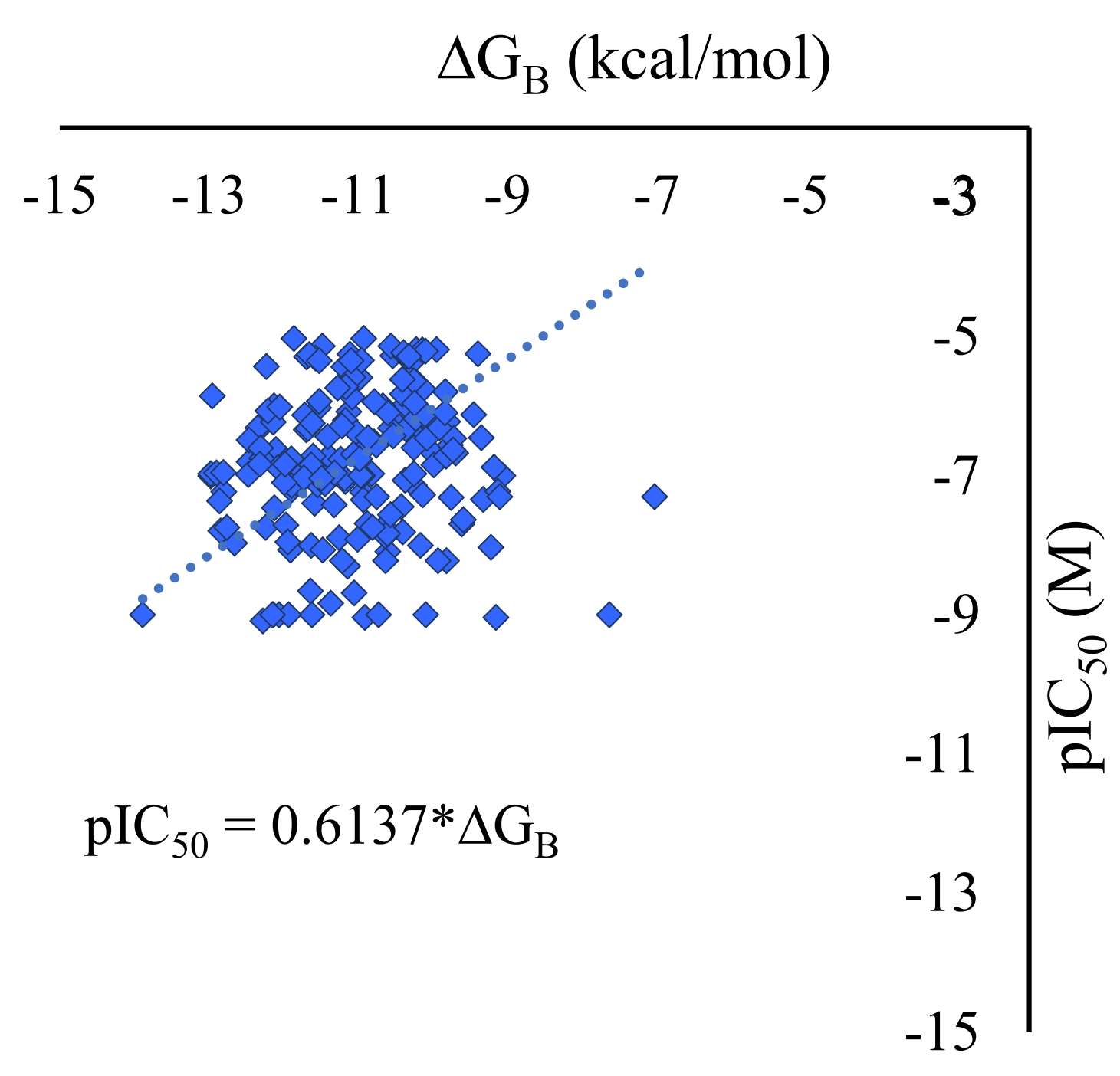
Figure 2.
Interaction profiles of the best-docked poses for the A) CNP0035993 (unclassified), B) CNP0386002 (plants), C) CNP0133095 (fungi), D) CNP0144730 (marine), and E) BMS-200 (positive control) with the calculated ΔGB of -13.988 kcal/mol, -13.051 kcal/mol, -12.541 kcal/mol, -11.716 kcal/mol and -11.866 kcal/mol, respectively. BMS-202 also has IC50 determined by the homogeneous time-resolved fluorescence (HTRF) binding assay [33].
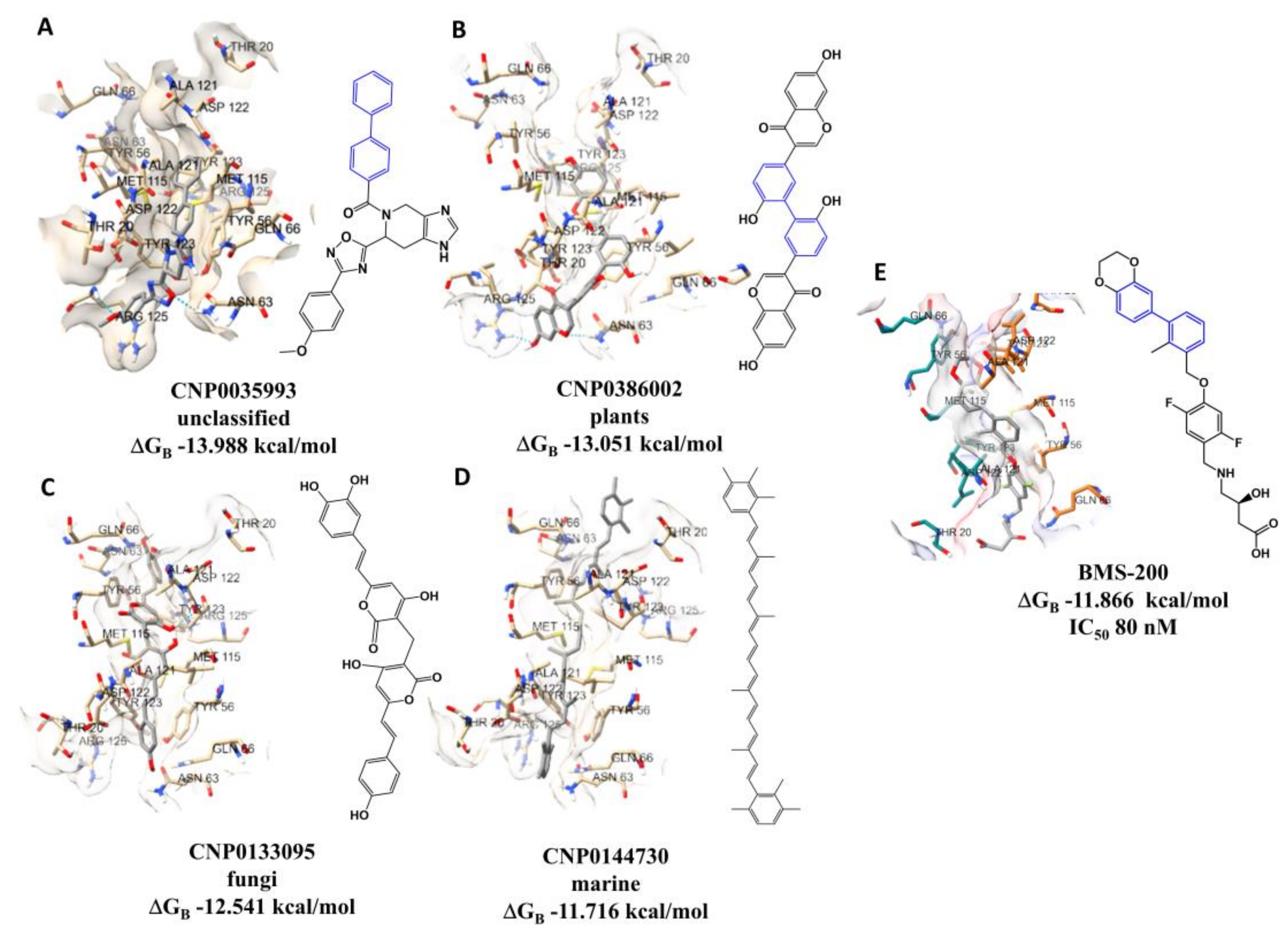
Figure 3.
Source origin distribution of the dataset extracted from the COCONUT database.
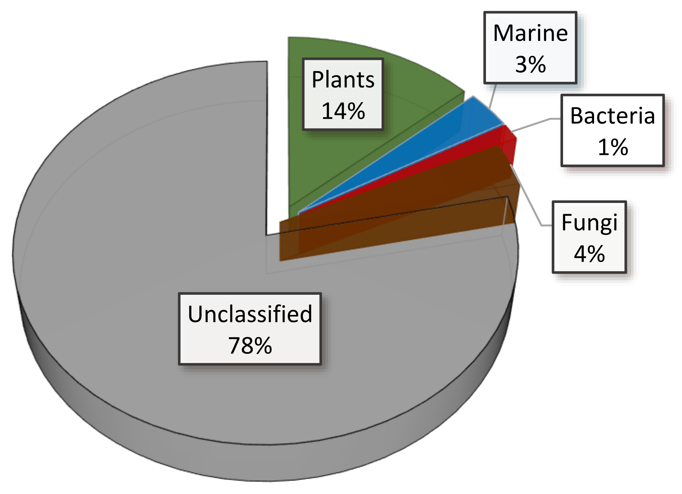
Figure 4.
Predicted vs calculated of the pIC50 for the ligand-PD-L1 complex for the 119,733 molecular structures of the training set (results obtained with the LightGBM using the 150 most important NMR SPINUS spectral descriptors).
Figure 4.
Predicted vs calculated of the pIC50 for the ligand-PD-L1 complex for the 119,733 molecular structures of the training set (results obtained with the LightGBM using the 150 most important NMR SPINUS spectral descriptors).
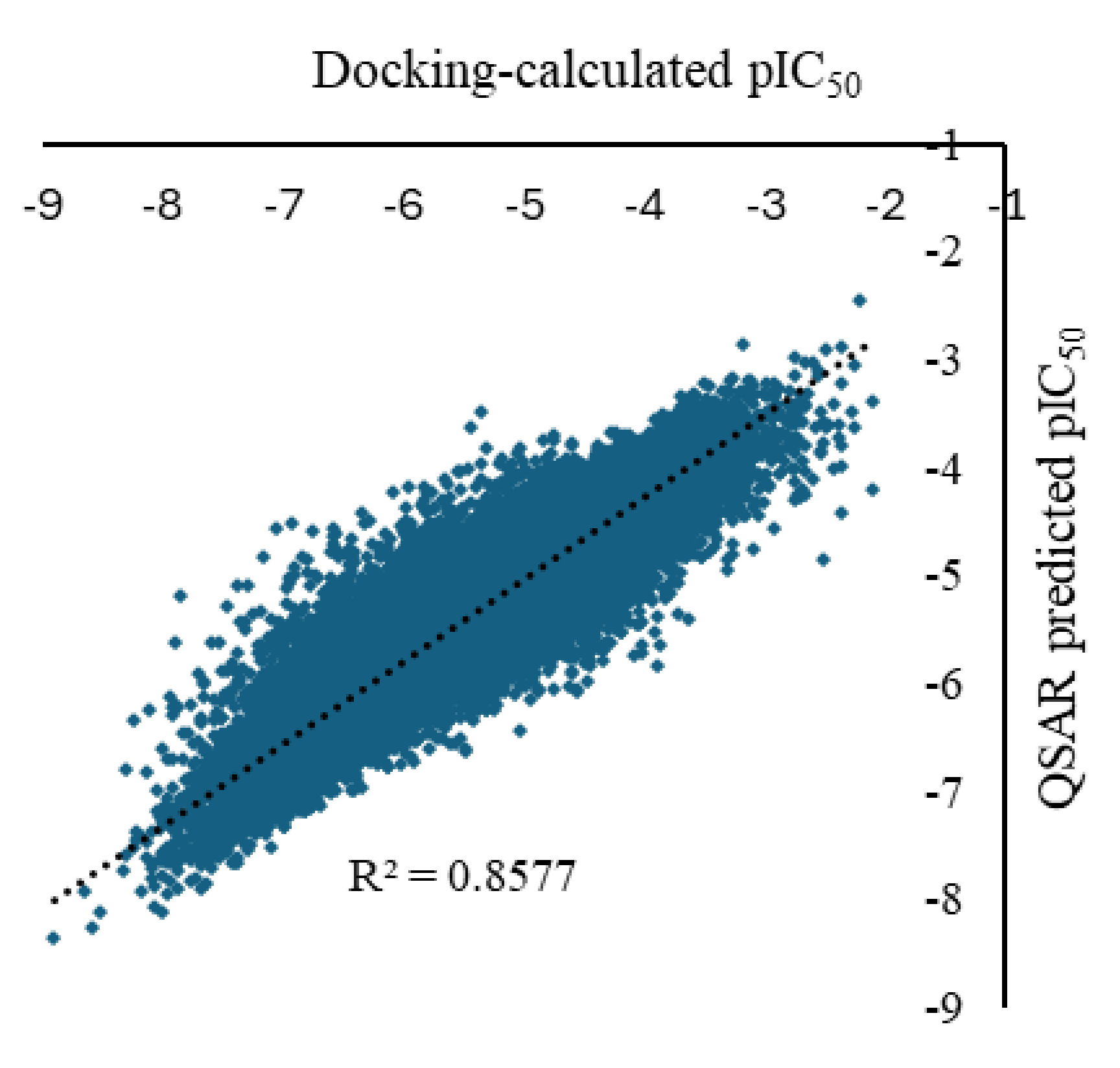
Figure 5.
Predicted vs calculated of the pIC50 for the ligand-PD-L1 complex for the 1,202 molecular structures of the external test set (results obtained with the LightGBM using the 150 most important NMR SPINUS spectral descriptors).
Figure 5.
Predicted vs calculated of the pIC50 for the ligand-PD-L1 complex for the 1,202 molecular structures of the external test set (results obtained with the LightGBM using the 150 most important NMR SPINUS spectral descriptors).
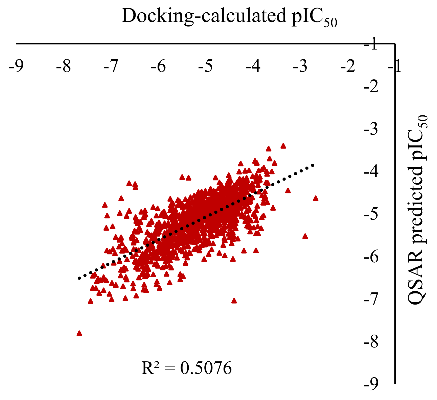
Figure 6.
A plot of the average TC values against the MAE of the QSDAR model prediction. Where: # TCAVE < - the number of molecules with an avereage TC value less than a given value; # TCAVE >= - the number of molecules with an average TC value greater than or equal to a given value.
Figure 6.
A plot of the average TC values against the MAE of the QSDAR model prediction. Where: # TCAVE < - the number of molecules with an avereage TC value less than a given value; # TCAVE >= - the number of molecules with an average TC value greater than or equal to a given value.
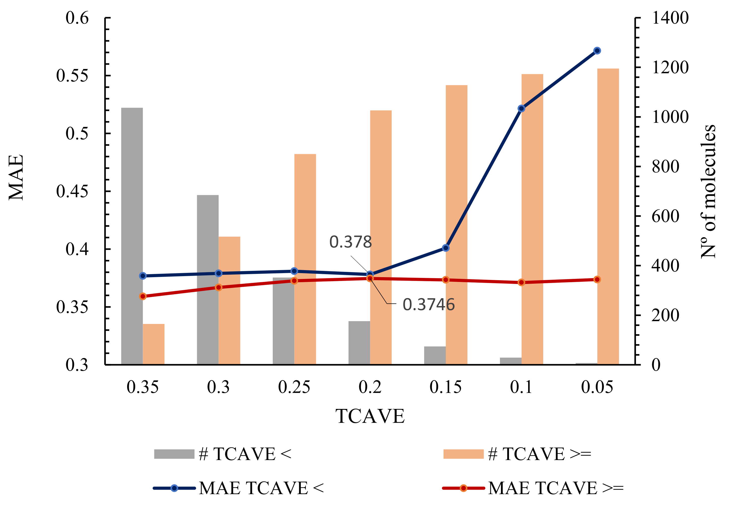
Figure 7.
Interaction profiles of the best-docked poses for A) two top-performing predictions: CNP0407375 and CNP0000488; and for B) two outliers predictions: CNP0334425 and CNP0179696.
Figure 7.
Interaction profiles of the best-docked poses for A) two top-performing predictions: CNP0407375 and CNP0000488; and for B) two outliers predictions: CNP0334425 and CNP0179696.
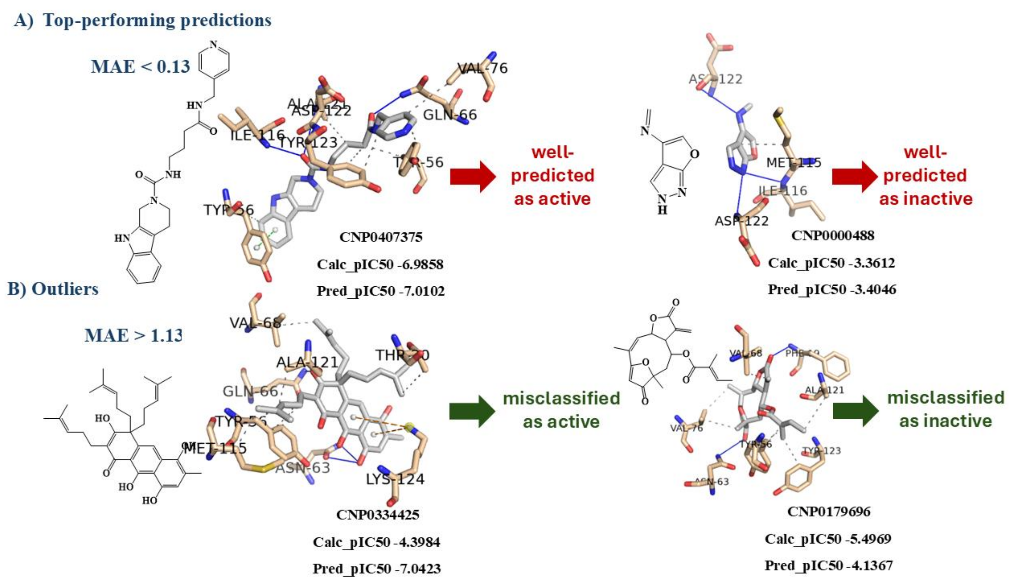

Table 1.
PD-L1 activity classes, drug-likeness characteristics and NP-likeness score for the training and test sets.
Table 1.
PD-L1 activity classes, drug-likeness characteristics and NP-likeness score for the training and test sets.
| Sets | # | PD-L1 Activity | Drug-likeness | NP-likeness score5 | ||
|---|---|---|---|---|---|---|
| Active1 | Inactive2 | MWheatom3 | MolLogP4 | |||
| Training | 119,733 | 62,651 (52%) |
57,082 (48%) |
112,555 (94%) |
100,534 (84%) |
52,640 (44%) |
| Test | 1,202 | 655 (54%) |
547 (46%) |
1,141 (95%) |
1,004 (84%) |
519 (43%) |
Table 2.
Evaluation of the predictive performance of the two spectral descriptors for modelling the PD-L1 activity using the RF algorithm for the training set in OOB estimation. The best model is highlighted in bold.
Table 2.
Evaluation of the predictive performance of the two spectral descriptors for modelling the PD-L1 activity using the RF algorithm for the training set in OOB estimation. The best model is highlighted in bold.
| Spectral Descriptors | #1 | R2 | MAE3 | RMSE4 |
|---|---|---|---|---|
| SPINUS | 570 | 0.8822 | 0.225 | 0.302 |
| GNN | 250 | 0.7632 | 0.310 | 0.395 |
| SPINUS + GNN | 820 | 0.9112 | 0.198 | 0.263 |
1 N.º descriptors. 2Coefficient of determination squared. 3Mean absolute error. 4Root mean squared error.
Table 3.
Spectral descriptor selection of NMR SPINUS set for the QSDAR RF model of the PD-L1 activity for the training set in OOB estimation. The best model is highlighted in bold.
Table 3.
Spectral descriptor selection of NMR SPINUS set for the QSDAR RF model of the PD-L1 activity for the training set in OOB estimation. The best model is highlighted in bold.
| Model | #1 | R2 | MAE3 | RMSE4 |
|---|---|---|---|---|
| SPINUS | 50 | 0.7142 | 0.333 | 0.432 |
| 100 | 0.7872 | 0.293 | 0.382 | |
| 150 | 0.8822 | 0.225 | 0.302 | |
| 200 | 0.8412 | 0.259 | 0.339 |
1 N.º descriptors. 2Coefficient of determination squared. 3Mean absolute error. 4Root mean squared error.
Table 4.
Exploration of diverse ML algorithms using the 150 most important descriptors (NMR SPINUS spectral descriptors) for both the training set and test set. The ML technique exhibiting the most optimal performance is highlighted in bold.
Table 4.
Exploration of diverse ML algorithms using the 150 most important descriptors (NMR SPINUS spectral descriptors) for both the training set and test set. The ML technique exhibiting the most optimal performance is highlighted in bold.
| Model | R2 | MAE2 | RMSE3 |
|---|---|---|---|
| Training set | |||
| RF4 | 0.8821 | 0.225 | 0.302 |
| LightGBM5 | 0.8581 | 0.219 | 0.296 |
| SVM5 | 0.5881 | 0.341 | 0.488 |
| CNN5 | 0.59301 | 0.3530 | 0.4835 |
| Test set | |||
| RF4 | 0.4921 | 0.406 | 0.547 |
| LightGBM5 | 0.5081 | 0.393 | 0.537 |
| SVM5 | 0.4041 | 0.450 | 0.591 |
| CNN5 | 0.45971 | 0.4241 | 0.5611 |
1Coefficient of determination squared. 2Mean absolute error. 3Root mean squared error. 4OOB estimation. 510-Fold cross-validation estimation.
Table 5.
Evaluation of the predictive performance of FPs, 1D&2D and 3D molecular descriptors for modelling the PD-L1 activity using the LightGBM algorithm for the training set in 10-fold cross-validation estimation. The best models are highlighted in bold.
Table 5.
Evaluation of the predictive performance of FPs, 1D&2D and 3D molecular descriptors for modelling the PD-L1 activity using the LightGBM algorithm for the training set in 10-fold cross-validation estimation. The best models are highlighted in bold.
| Descriptors | #1 | R2 | MAE3 | RMSE4 | |
|---|---|---|---|---|---|
| FPs | MACCS | 166 | 0.86642 | 0.1982 | 0.2762 |
| Morgan | 1024 | 0.962 | 0.1041 | 0.144 | |
| RDKit | 2048 | 0.972 | 0.0812 | 0.1317 | |
| 1D&2D | 425 | 0.992 | 0.0179 | 0.0269 | |
| 3D | Autocorr3D | 80 | 0.99472 | 0.0393 | 0.0548 |
| Getaway | 271 | 0.992 | 0.0139 | 0.02 | |
| RDF | 210 | 0.992 | 0.0213 | 0.0308 | |
| 3D | 561 | 0.992 | 0.0096 | 0.0139 | |
| Quantum | 5 | 0.65892 | 0.3513 | 0.4484 | |
1 N.º descriptors or FPs. 2Coefficient of determination squared. 3Mean absolute error. 4Root mean squared error.
Table 6.
Prediction of the LightGBM ML algorithm with 1D&2D and 3D descriptors for both training set and test set.
Table 6.
Prediction of the LightGBM ML algorithm with 1D&2D and 3D descriptors for both training set and test set.
| Model | #1 | R2 | MAE3 | RMSE4 |
|---|---|---|---|---|
| Training set5 | ||||
| 1D&2D&3D | 986 | 0.992 | 0.0075 | 0.0111 |
| Test set | ||||
| 1D&2D&3D | 986 | 0.81312 | 0.2493 | 0.3283 |
1N.º descriptors. 2Coefficient of determination squared. 3Mean absolute error. 4Root mean squared error. 510-Fold cross-validation estimation.
Table 7.
Hyperparameter settings of the best dMLP model.
| Hyperparameter | Setting |
|---|---|
| Initializer | Glorot uniform |
| Number of hidden layers | 4 |
| Number of neurons in the 1st, 2nd, 3rd and 4th layers | 150 |
| Activation 1st–3rd layers | Relu |
| Activation 4th layer | Relu |
| Batch size | 128 |
| Optimizer | Adam |
| Epochs | 500 |
Disclaimer/Publisher’s Note: The statements, opinions and data contained in all publications are solely those of the individual author(s) and contributor(s) and not of MDPI and/or the editor(s). MDPI and/or the editor(s) disclaim responsibility for any injury to people or property resulting from any ideas, methods, instructions or products referred to in the content. |
© 2025 by the authors. Licensee MDPI, Basel, Switzerland. This article is an open access article distributed under the terms and conditions of the Creative Commons Attribution (CC BY) license (http://creativecommons.org/licenses/by/4.0/).
Copyright: This open access article is published under a Creative Commons CC BY 4.0 license, which permit the free download, distribution, and reuse, provided that the author and preprint are cited in any reuse.


