
Submitted:
24 March 2025
Posted:
25 March 2025
You are already at the latest version
Preprints on COVID-19 and SARS-CoV-2
Abstract
Robust control of the four-link manipulator arm (FLMA) is an important subject for many industrial applications such as COVID-19 prevention robotics, lower limb rehabilitation robotics and underwater robotics. This study uses the feedback linearized approach to stabilize the complex nonlinear FLMA without applying nonlinear approximator that includes the fuzzy approach and the neural network optimal approach. The article proposes a new approach based on the “first” derived nonlinear convergence rate formula of FLMA to control the highly nonlinear dynamics. The linear quadratic regulator (LQR) method is often applied in the balance controlling space of the underactuated manipulator. This proposed approach takes the place of LQR approach without the necessary trial and error operations. The implications of proposed approach are “globally” valid, whereas the Jacobian linearized approach is “locally” valid. In addition, the main innovation of the proposed method is to perform “simultaneously” additional performances including the almost disturbance decoupling performance that takes the place of the traditional posture-energy approach and avoids some torque chattering behaviour in the swing-up space, and globally exponential stable performance without solving the Hamilton-Jacobin equation. Comparative examples show that the proposed controller is superior to the singular perturbation and the fuzzy approaches.
Keywords:
almost disturbance decoupling performance
; COVID-19 prevention robotics
; feedback linearized approach
; four-link manipulator arm
; nonlinear convergence rate
1. Introduction
The automation of manipulator arm has gained tremendous attention in recent decades due to their wide range of engineering applications, such as agricultural mobile robotics [1], mining mobile robotics [1], space exploration mobile robotics [2], lower limb rehabilitation robotics [3], biped walking robotics [4[, unmanned ground vehicle [5] and underwater robotics [6]. There are two types of manipulator arm: underactuated one [7,8,9], which is a kind of a nonlinear system with fewer control inputs than degrees of freedom, and fully actuated one [5,6,10,11], which is not. In general, underactuated manipulator arms are grouped into vertical types which are controlled by gravity and planar types which are not.
For the vertical underactuated manipulator, the linear Jacobian approximated model of the inverted equilibrium position is completely controllable because the controllability matrix of the linear Jacobian approximated model is full rank. For most traditional approaches of solving the complexity of vertical underactuated manipulator, the operation space is mainly separated into a swing-up space and a balance space. In the swing-up space, the control methods include posture-energy approach [12], energy-based approach [13], direct fuzzy control approach [11], fuzzy model reference learning control approach [11], adaptive fuzzy control approach [11], and then the linear quadratic regulator (LQR) optimal method [14] is applied in the balance space. However, to be quickly captured in the swing-up space for the manipulator arm, the control needs to be built an exact combination of energy and posture, and this property is difficult to be accomplished due to the complexity of the system dynamics [9]. Moreover, some torque chattering change occurs in the swing-up space and then the energy is quickly pumped into the system [9]. In general, in order to control the nonlinear dynamics well, the disturbance decoupling and the global stability should be simultaneously required [15]. To achieve these requirements, some significant approaches, such as model predictive control [16], deep rcement learning [17], multi-objective control [18], backstepping control [19] and preview control [20], have been adopted for complex nonlinear systems. However, in the aforementioned approaches, a serious common drawback is that the considered nonlinear systems should be approximated to be linear dynamics by the Taylor expansion for small effect operating range. This serious drawback may be impractical for the FLMA. To solve nonlinear serious drawback of the FLMA, nonlinear function approximators, such as neural network optimal approach [21] and famous fuzzy method [22], have been adopted to reduce the caused errors [23]. The main drawback of famous fuzzy method is that constructing fuzzy rule base needs to rely on many past accumulated knowledges, and then the system performance is almost determined by the constructed experience rule base [24]. The neural network optimal approach is an intelligent supervised learning approach that requires the operating network to offer many sample points [25]. The performance of controller design for the neural network method is completely limited by only applying the current state value. Moreover, complicated interconnecting structure and digital computing loads let the physical realization of nonlinear function approximators be impractical. LQR is a common method that calculates the weighting matrices Q and R for a Jacobian linearized system via trial and error operation. Some improved approaches of calculating the weighting matrices, such as genetic algorithm approach and Kalman’s pole-assignment approach, have been proposed in recent decades. However, their main serious drawbacks including high computing effort and slowly convergent rate of globally optimal solution limit their performances [26].
On the other hand, planar underactuated manipulator is not constrained by gravity, so any position of the manipulator arm is the equilibrium point and the linear Jacobian approximated model at any equilibrium point is uncontrollable [27]. The control approaches for the vertical underactuated manipulator cannot be applied for planar underactuated manipulator. The researches of controlling planar underactuated manipulator are extensive and some important methods, such as the nilpotent approximated method [28], the converting-chained form method [29] and the order-reduction method [30], have been proposed to perform the position control for planar underactuated manipulator. However, the aforementioned approaches of controlling the planar underactuated manipulator are only valid for the nominal plant model. In real systems, nonlinear acting factors need to be considered [31] and then aforementioned approaches cannot be applied for the practical planar underactuated manipulator.
So far, it is obvious to see that the robust and tracking controller design for manipulator arm still is a challenging subject due to the strict global stability requirement and disturbances reduction involving on the nonlinear system dynamics. Stimulated by these points, we apply feedback linearized approach to construct the robust and tracking controller of manipulator arm with the almost disturbance decoupling, adjustable convergence rate and “globally” exponentially stable performances and take the place of “locally” Jacobian linearized method. Feedback linearized approach have contributed many significant researches [32,33,34,35,36] in industrial applications, such as the dual parallel-PMSM system [32], the grid-tied packed e-cell inverter [33], PHEVs charging station [34], artificial pancreas [35] and the weak AC grid integration [36].
References [37,38] had exploited the fact that the stricter tracking error condition of almost disturbance decoupling performance including absolute error, integral error and input-to-state-stable error is involved to reduce the disturbance effect. However, they can only achieve the almost disturbance decoupling performance of nonlinear system without the nonlinearity multiplied with disturbance requirement and the non-Lipschitz nonlinearity requirement. Therefore, the almost disturbance decoupling performance cannot be achieved for the following nonlinear system:,, , whereandare the output and control input, respectively. On the contrary, the almost disturbance decoupling performance can be well achieved by the proposed method. The main novelty of this study is to design robust and tracking controller for nonlinear complex FLMA. Major contributions of this study are summarized as follows:
(i) This study has “first” presented the convergence rate formula of the nonlinear FLMA.
(ii) The FLMA is first designed by applying the feedback linearized approach with the almost disturbance decoupling performance that takes the place of the traditional posture-energy approach and avoids some torque chattering change behaviour in the swing-up space. Moreover, the proposed approach takes the place of LQR approach without the necessary trial and error operations.
(iii)A robust and tracking controller is presented to possess the global exponential stability without solving the Hamilton-Jacobi equation that requires to be solved for the famous H-infinity approach.
(iv)The study has proposed a new approach to improve the shortcoming of traditional fuzzy function approximators without many design experiences and knowledges.
(v)The implications of this proposed method are “globally” valid, whereas the Jacobian linearized approach is “locally” valid.
2. Complete Mathematical Model for Four-link Manipulator Arm
The FLMA is a great platform for industrial mechanics as it is highly nonlinear control system with disturbances. In this section, we will apply Euler-Lagrange equation to derive the dynamic equations of the FLMA shown in Figure 1.
Four-link manipulator arm is made up of aluminum. The dynamic model parameters are selected as follows: the length of link, the distance for the center of mass, the mass of linkand the inertia moment of link. Defining the potential energy, the kinetic energy, the joint torque, the Lagrangian termas the difference between the kinetic energy and potential energy, and applying the Euler–Lagrange equation yield the dynamic equation of the FLMA to be
Let the centroid translational position vector and velocity vector of linkbeand , and centroid rotational position vector and velocity vector of linkbe and. From the fundamental definitions of position vector and velocity vector, we get
and
Then the kinetic energyof the manipulator arm will be given by
Define
Substituting (10)~(12) to (9) obtains
From (1)(2) and (13), we get
Then
Since the matrixpossesses positive definite property and, we get
i.e.
Define
and
From (17)~(19), it is more practical to rewrite the Euler–Lagrange equation of the manipulator arm in more compact form for control purpose as follows:
whereis the vector of gravity force,denotes the Coriolis matrix of the manipulator arm. Observing the structure of (19) obtains
where
Define
and
Then (12) can be rewritten to be
Observing Figure 1 yields the centroid translational position vector to be ,,and
whereand.,,,. Applying (6) to the centroid translational position vector gets
Observing Figure 1 yields the centroid rotational position vector to be, , and. Using (8) to the centroid rotational position vector obtains
Substituting (24)~(25) and (27)~(34) to (25) yields the matrixas
where
Let us combine (21) and (22) and get the matrix as
where
Using (35) yields the inverse of the matrixto be
where
From (43) and (63), we get
where
Multiplying (63) with (19) yields
where
From (20), we obtain
Substituting (63), (72) and (87) to (92) gets
Define the state, input and noise variables of the FLMA to be the following physical quantities: ,,,,,,,,,,, , and .
Therefore, the state-space dynamic model of the FLMA with real physical values can be represented as
<i> The following condition holds:
for all,, where the symbolis the Lie operator.
<ii>The square matrix
has nonsingular property. The norms of pre-specified tracking signalsand its firstderivatives are bounded by positive constantsas
and the spanning distribution
is involutive.
3. Robust and Tracking Controller Design of the FLMA System
Since the FLMA system has the well-defined relative degree property and involutive distribution performance, then the mapping
defined as
and
is an one-to-one and onto, infinitely continuous and differentiable function according to reference [39,40], i.e,
Assume that the nonlinear FLMA system possesses the well-defined involutive property. Then the mapping defined by (124)~(127) is a one-to-one and onto, infinitely continuous and differentiable function and it will transform original nonlinear system into partially linear subsystem and partially nonlinear subsystem as follows [39,40] as follows:
Since
the transformed dynamics of nonlinear FLMA system (139)~(145) can be rewritten to be
Hence
Then we can transform (152) into the following model
From (158), we get
Next we will demonstrate in detail how to design the robust and tracking controllewith the pre-specified tracking signals. The initial values of the states are set to be
The desired robust and tracking controller is built by
whereis the desired tracking signal andare elements of the Hurwitz matrix shown by
Based on feedback linearization approach, then we propose the robust controller with the pre-specified tracking signalsas follows:
For the convenience of the following discussions, let’s define some related parameters as
where the Lyapunov system matrixis a Hurwitz matrix whose eigenvalues lies in the left half coordinate plane and one can use Matlab to obtain the adjointing Lyapunov system matrixof the following Lyapunov equation:
and
To demonstrate further the complete feedback linearization control design of nonlinear FLMA system, let’s define one assumption and two definitions as
Assumption 1. The following inequality holds:
whereand.
Definition 1. Consider a nonlinear systemwith an Lipschitz input, whereis Lipschitz state variable,is differentiable and infinitely continuous. This system is defined to be input-to-state stable if
whereis a-class function anddenotes a-class function.
Definition 2. A nonlinear system with noise inputis defined to possess the almost disturbance decoupling performance, if the following properties hold:
<i>The nonlinear system has input-to-state stable property for noise input.
<ii>Output tracking errors meet the following two inequalities for initial timeand the initial state:
and
where belongs to -class function,andare positive constants, and, belong to -class functions. From (159), we get
From (171),(173) and (188), we obtain
Substituting (161) and (162) into (189) obtains
Then, from (145), (153), (162), (174) and (190), we obtain
where
It is worth noting that the one-to-one and onto, infinitely continuous and differentiable function converts the original nonlinear FLMA into a partially nonlinear subsystem and partially linear subsystem whose state variables are denoted byand, respectively. In order to meet the requirements (184) and
we constructandto be the Lyapunov functions of nonlinear subsystem (192) and linear subsystem (191), respectively and then combine these Lyapunov functions to be a composite Lyapunov functionas follows:
where the functionsatisfiesand
Then, the differentiation of the composite Lyapunov function is described as
where the matrixis positive definite, and
i.e.
wheredenotes the minimum eigenvalue of the matrix.
Define
Applying (217) into (216) yields
Define
and get
Next, we will prove the fact that the proposed feedback linearization control achieves the almost disturbance decoupling performance, and the globally exponential stability of the FLMA system in Appendix A. Therefore, the proposed robust tracking control (163) will indeed drive the tracking errors of the FLMA system into the global ultimate attractor.
Noting that we can extend above complete design process to obtain one more general significant theorem for general uncertain nonlinear control systems with disturbances as follows:
i.e.,
where,denote the input and output, respectively,is the state variable, is the noise vector,denotes the noise_adjoint vector. Assume, and to be continuous functions, andto be the matched uncertainty vector term, whereis defined to be the uncertainty vector.
Assumption 2. The following inequality holds:
whereand.
<i>The following condition holds:
for all,, where the symbolis the Lie operator.
<ii>The square matrix
has nonsingular property. The norms of pre-specified tracking signalsand its firstderivatives are bounded by positive constantsas:
and the spanning distribution
is involutive. Then the mappingdefined as
and
is an one-to-one and onto, infinitely continuous and differentiable function according to reference [39].
Letandbe the Lyapunov functions of nonlinear subsystem and linear subsystem, respectively and then combine these Lyapunov functions to be a composite Lyapunov functionas follows:
Theorem 1. A differentiable and infinitely continuous functionfor transformed nonlinear subsystem can be found to make the following three inequalities hold:
Design the robust and tracking controller to be
Then the nonlinear system possesses the almost disturbance decoupling performance with the globally exponential stability:
where the matrixis positive definite, and the continuous function satisfiesand
Moreover, the desired tracking errors can be exponentially reduced by adjusting the parameterwith the convergence rate formula
and the desired tracking errors of control system are exponentially attracted into a global final attractorwith the convergence radius formula
To effectively build robust and tracking controller, a significant algorithm of FLMA is summarized as follows, and then a powerful Python software system of controller design is constructed in the next section according to this proposed algorithm.
(Step 1)Obtain the vector relative frequencyaccording to the given outputs.
(Step 2)Appropriately construct the one-to-one and onto, infinitely continuous and differentiable functionbased on (123)~(127).
(Step 3)From (162) and (178), appropriately choose parameterssuch thatare Hurwitz matrices with stable eigenvalues and obtain the positive definiteof the Lyapunov equation with the aid of Matlab toolbox.
(Step 4)Choose the Lyapunov functionto meet the requirements (184) and (198)~(200). If the vector relative frequency is equal to the system dimension, i.e. , then this step will be omitted and directly go to (Step 5).
(Step 5)From (212)~(215), (217)~(220), appropriately design parameters to meet. It is worth noting that if the value ofis larger, the convergence rate is faster.
(Step 6)Finally, the robust and tracking controller can be built by (163).
4. Simulations of the FLMA System
It can be verified that the related requirements of Theorem 1 hold if we choose,,,,,,,,. Hence the robust and tracking controller will make the tracking errors converge to the globally final attractor by Theorem 1. The real tracking errors of the FLMA system (epsion=0.01) are plotted in Figure 2. Therefore, the designed controller can indeed make the outputs track the pre-specified signals. From (260)~(261) and Figure 2 and Figure 3, it is obvious to see that the convergent rate of tracking error with smaller epsion is better than a larger epsion. Moreover, the dynamic trajectories show the overall tracking errors “before”, “on” and “after” entering the globally final attractor in the positive z direction for Figure 4, Figure 5 and Figure 6, respectively, where the length of the arrow denotes the convergence-radius of the globally final attractor. Other individual tracking errors of the output 1~output 4 are shown in positive x direction, negative x direction, positive y direction and negative y direction for Figure 4, Figure 5 and Figure 6, respectively.
5. Comparisons to Traditional Approaches
In this section, we will compare the performance of proposed approach with traditional fuzzy approach [41] and the singular perturbation method with high-gain feedback [38].
Figure 7 is the general structure of traditional fuzzy approach whose input variables of the IF-THEN rules are assigned to be the tracking errorand its time derivative. The output variable is the fuzzy control. For easy calculation, the desired membership functions of,andare assigned to be the triangular shape functions as shown in Figure 8, Figure 9 and Figure 10. The desired fuzzy control rule base foris constructed in Table 1. The rule base, fuzzy inference engine and defuzzifier adopt the standard Macvicar-Whelan rule base, the Mamdani method and the centroid method, respectively.
With the aid of Matlab fuzzy toolbox, comparative tracking error responses of the proposed approach and traditional fuzzy controller design for the FLMA are shown in Figure 11, Figure 12, Figure 13 and Figure 14. From Figure 11, Figure 12, Figure 13 and Figure 14, it is obvious to see that the convergence rate of the proposed approach is faster than the traditional fuzzy approach.
Following the second comparative example, we will make some comparison between the proposed approach and the famous singular perturbation method [37,38]. The sufficient condition in [37,38] needs that the nonlinearity multiplied by the disturbance meets the structural triangle criterion.
References [37,38] had exploited the fact that the following system cannot achieve the almost disturbance decoupling performance:
It is easy to derive the following items:,, , and
Hence the sufficient condition of [37,38] is not satisfied sinceis not complete, and then the almost disturbance decoupling problem cannot be not solved. On the contrary, this almost disturbance decoupling problem can be solved via the proposed approach by the controller
The output response of the nonlinear system for (263) is shown in Figure 15. Therefore, the designed controller can indeed make the output track the pre-specified signalsand achieve the almost disturbance decoupling performance.
6. Conclusion
Continuous spreading COVID-19 virus stimulates us to design the robust controller of the highly nonlinear FLMA by the feedback linearized approach that possesses almost disturbance decoupling performance taking the place of the traditional posture-energy approach and avoiding torque chattering change behaviour in the swing-up space, and other globally exponential stability performance without solving the famous Hamilton-Jacobin equation. The disturbance has a sensitive effect on FLMA and then this article addresses stricter disturbance requirements including absolute value error, integration error and input-to-state stable condition.
This study derives successfully the nonlinear convergence rate formula of the FLMA and the related convergence radius of the globally final attractor. Moreover, in order to clearly show that dynamic trajectories of the output tracking-errors for the nonlinear FLMA system converge to the global final attractor, one Matlab software are completely designed to demonstrate the tracking-error trajectories before, on and after entering the globally final attractor.
The simulation results of two demonstrative examples show that the convergence rate using proposed controller is faster than using traditional fuzzy controller, and superior to the traditional singular perturbation approach.
Author Contributions
Conceptualization, Kuang-Hui Chi; methodology, Chung-Cheng Chen; software, Yung-Feng Hsiao; validation, Yung-Feng Hsiao; formal analysis, Yung-Feng Hsiao; investigation, Yung-Feng Hsiao; resources, Kuang-Hui Chi; data curation, Kuang-Hui Chi; writing—original draft preparation, Chung-Cheng Chen; writing—review and editing, Kuang-Hui Chi and Yung-Feng Hsiao; visualization, Kuang-Hui Chi; supervision, Chung-Cheng Chen; project administration, Kuang-Hui Chi and Chung-Cheng Chen.
Data Availability Statement
No new data were created or analyzed in this study. Data sharing is not applicable to this article.
Conflicts of Interest
The authors declare no conflicts of interest.
Appendix A
In Appendix A, we will prove that the nonlinear FLMA system with the proposed control can achieve the three almost all disturbance decoupling performances, the convergent radius formula and the globally exponential stability. First, applying (224) easily gets
In Appendix A, we will prove that the nonlinear FLMA system with the proposed control can achieve the three almost all disturbance decoupling performances, the convergent radius formula and the globally exponential stability. First, applying (224) easily gets
i.e.
Integrate both sides of the inequality (A.2) to get
i.e.
Therefore,
Similarly, we can extend above result to be
and then we can conclude that the third almost disturbance decoupling requirement is achieved. Next, we will achieve the first almost disturbance decoupling performance. (222) can be rewritten as
Let
Combining (A.7) and (A.8) yields
Then
Therefore, the state trajectory lying in the outside of the global ultimate attractor is described by
Then
From (181), (198), (201) and (204), we get
Defineand we can get
Similarly, we can achieve
Defineand we can obtain
Combining (A.14) and (A.16) gets
From (A.11)-(A.12) and (A.17) and the input-to-state stable theorem [40], we can conclude that the first almost disturbance decoupling requirement is achieved. Next, we will achieve the first almost disturbance decoupling performance. Combining (A.7), (A.8), (A.17) and (219) gets
Applying the comparison theorem to (A.18) yields
Then we can get
and
Observing (A.21) verifies the second almost disturbance decoupling requirement and the convergence rate of tracking errors is . It is obvious to see that we can change the value of to adjust the convergence rate. Moreover, from (A.7), (A.8) and (219) , we get
Considering the output trajectory for yields , and then any sphere
will be a global final attractor of the nonlinear FLMA system with the convergent radius .
Next, we will verify the globally exponential stability of the nonlinear FLMA system. Combining (A.17) and (A.19) yields
and
Then
Hence we can achieve the globally exponential stability of the global final attractor.
References
- S. A. Marinovic, M. T. Torriti and F. A. Cheein, “General dynamic model for skid-steer mobile manipulators with wheel-ground interactions,” IEEE/ASME Trans. Mechatronics, vol. 22, no. 1, pp. 433–444, Feb. 2017.
- Z. Li and S. S. Ge, Fundamentals in modeling and control of mobile manipulators. Boca Raton, FL, USA: CRC Press, 2013.
- J. Wu, J. Gao, R. Song, R. Li, Y. Li and L. Jiang,“The design and control of a 3 DOF lower limb rehabilitation robot”, Mechatronics, vol. 33, pp. 13-22, 2016. [CrossRef]
- X. Wang, H. Zeng and H. Zhou, " A spatial four-link 4R biped walking mechanism," in 2019 IEEE 9th Annual International Conference on CYBER Technology in Automation, Control, and Intelligent Systems, Suzhou, China, July, 2019, pp. 203-208.
- M. U. Masood, M. Mujtaba, M. A. Sami, N. Rashid and J. Iqbal, "Design and experimental testing of an in-parallel actuated 3 DOF serial robotic manipulator for unmanned ground vehicle," in 2018 3rd Asia-Pacific Conference on Intelligent Robot Systems (ACIRS), Singapore, Singapore, July, 2018, pp. 45-49.
- F. Leborne, V. Creuze, A. Chemori, L. Brignone and J. Iqbal,"Dynamic modeling and identification of an heterogeneously actuated underwater manipulator arm," in 2018 IEEE International Conference on Robotics and Automation (ICRA), Brisbane, Australia, May, 2018, pp. 4955-4960.
- M. Reyhanoglu, A. van der Schaft, N. H. Mcclamroch and I. Kolmanovsky, "Dynamics and control of a class of underactuated mechanical systems," IEEE Transactions on Automatic Control, vol.44, no. 9, pp. 1663 – 1671, 1999. [CrossRef]
- X. Lai, Y, Wangm, M. Wu and W. Cao, “Stable Control Strategy for Planar Three-Link Underactuated Mechanical System,” IEEE/ASME Transactions on Mechatronics, vol. 21, no., 3, pp. 1345 – 1356, 2016. [CrossRef]
- X. Z. Lai, A. C. Zhang, J. H. She, and M. Wu, “Motion control of underactuated three-link gymnast robot based on combination of energy and posture,” IET Control Theory Appl., vol. 5, no. 13, pp. 1484–1492, 2011. [CrossRef]
- M. R. Thompson, M. T. Torriti, F. A. Auat Cheeina and G. Troni, “H∞-Based Terrain Disturbance Rejection for Hydraulically Actuated Mobile Manipulators With a Nonrigid Link,” IEEE/ASME Transactions on Mechatronics, vol. 25, no. 5, pp. 2523 - 2533, 2020.
- S. C. Brown and K. M. Passino, “Intelligent control for an acrobat,” J. Intell. Robot. Syst., vol. 18, no. 3, pp. 209–248, 1997.
- X. Z. Lai, A. C. Zhang, J. H. She, and M. Wu, “Motion control of underactuated three-link gymnast robot based on combination of energy and posture,” IET Control Theory Appl., vol. 5, no.13, pp. 1484–1493, 2011. [CrossRef]
- Fantoni, R. Lozano, and M. W. Spong, “Energy-based control of the pendubot,” IEEE Trans. Autom. Control, vol. 45, no. 4, pp. 725–729, 2002.
- B. Anditio, A. D. Andrini and Y. Y. Nazaruddin, " Integrating PSO Optimized LQR Controller with Virtual Sensor for Quadrotor Position Control," in 2018 IEEE Conference on Control Technology and Applications, Copenhagen, Denmark, August, 2018, pp. 1603-1607.
- J. Yang and Z. Ding, "Global output regulation for a class of lower triangular nonlinear systems: A feedback domination approach," Automatica, vol.76, pp. 65-69, 2017. [CrossRef]
- J. Wu, H. Zhou, Z. Liu and M. Gu, “Ride comfort optimization via speed planning and preview semi-active suspension control for autonomous vehicles on uneven roads,” IEEE Transactions on Vehicular Technology, vol. 69, no. 8, pp. 8343-8355, 2020. [CrossRef]
- M. Liu, Y. Li, X. Rong, S. Zhang and Y. Yin, “Semi-Active Suspension Control Based on Deep Reinforcement Learning,” IEEE Access, vol. 8, pp. 9978 - 9986, 2020.
- H. Chen, P. Y. Sun and K.-H. Guo, " A multi-objective control design for active suspensions with hard constraints," in 2003 Proc. Amer. Control Conf., 2003 pp. 4371–4376.
- J. S. Lin and C. J. Huang, “Nonlinear backstepping active suspension design applied to a half-car model,” Veh. Syst. Dyn., vol. 42, pp. 373–393, 2004. [CrossRef]
- C. Gohrle, A. Schindler, A. Wagner and O. Sawodny, “Design and vehicle implementation of preview active suspension controllers,” IEEE Trans. Control Syst. Technol., vol. 22, no. 3, pp. 1135–1142, 2014. [CrossRef]
- L. Tang, D. Ma and J. Zhao, “Adaptive neural control for switched non-linear systems with multiple tracking error constraints,” IET Signal Processing, vol. 13, no. 3, pp. 330 - 337, 2019. [CrossRef]
- L. Liu, Y. L. Liu, D. Li, S. Tong and Z. Wang, “Barrier Lyapunov function-based adaptive fuzzy FTC for switched systems and its applications to resistance–inductance–capacitance circuit system,” IEEE Transactions on Cybernetics, vol. 50, no. 8, pp. 3491 - 3502, 2020. [CrossRef]
- R. Cui, C. Yang, Y. Li and S. Sharma, “Adaptive neural network control of AUVs with control input nonlinearities using reinforcement learning,” IEEE Trans. Syst., Man, Cybern., Syst., vol. 47, no. 6, pp. 1019–1029, 2017. [CrossRef]
- D. Y. Wang and H.Wang, “Control method of vehicle semi active suspen-sions based on variable universe fuzzy control,” China Mech. Eng., vol. 28, no. 3, pp. 366-372, 2017.
- H. Li, Y. H. Feng and L. Su, “Vehicle active suspension vibration control based on robust neural network,” Chin. J. Construct. Mach., vol. 15, no. 4, pp. 324-337, 2017.
- Y. Y. Nazaruddin and P. Astuti, “Development of intelligent controller with virtual sensing”, ITB J. Eng. Sci , vol. 41, no. 1, pp.17-36, 2009. [CrossRef]
- M. Reyhanoglu, A. Schaft, and N. H. Clamroch, " Dynamics and control of a class of underactuated mechanical systems," IEEE Trans. Autom. Control. vol. 44, no. 9, pp. 1663–1671, 1999. [CrossRef]
- D. Luca, R. Mattone, and G. Oriolo, “Stabilization of an underactuated planar 2R manipulator,” Int. J. Robust Nonlinear Control, vol. 10, no. 4, pp. 181–1812, 2000.
- T. Yoshikawa, K. Kobayashi, and T. Watanabe, “Design of a desirable trajectory and convergent control for 3-DOF manipulator with a nonholonomic constraint,” in Proc. IEEE Int. Conf. Robot. Autom., San Francisco, , USA, 2000, vol. 2, no. 4, pp. 1805–18052.
- P. Y. Xiong, X. Z. Lai, and M.Wu, “A stable control for second-order nonholonomic planar underactuated mechanical system: Energy attenuation approach,” Int. J. Control, vol. 91, no. 7, pp. 1630–16302, 2018. [CrossRef]
- S. Zapolsky and E. Drumwright, “Inverse dynamics with rigid contact and friction,” Auton. Robots, vol. 41, no. 4, pp. 831–8312, 2017. [CrossRef]
- T. Liu, X. Ma, F. Zhu and M. Fadel, “Reduced-Order Feedback Linearization for Independent Torque Control of a Dual Parallel-PMSM system,” IEEE Access, pp. 1-1, 2021. [CrossRef]
- M. Mehrasa, M. Babaie, M. Sharifzadeh and K. A.Haddad, “An Input-Output Feedback Linearization Control Method Synthesized by Artificial Neural Network (ANN) for Grid-Tied Packed E-Cell Inverter,” IEEE Transactions on Industry Applications, pp. 1-1, 2021. [CrossRef]
- M. Awais, L. Khan, R. Badar, S. Mumtaz, S. Ahmad and S. Ullah, “Wavelet-Hybridized NeuroFuzzy Feedback Linearization based Control Strategy for PHEVs Charging Station in a Smart Microgrid, “ in 2020 International Symposium on Recent Advances in Electrical Engineering & Computer Sciences (RAEE & CS), Pakistan, Islamabad, Oct., 2020, pp. 1-6.
- S. A. Babar, I. Ahmad, I. S. Mughal and S. A. Khan, "Terminal Synergetic and State Feedback Linearization based Controllers for Artificial Pancreas in Type 1 Diabetic Patients," IEEE Access, pp. 1-1, 2021. [CrossRef]
- J. Khazaei, Z. Tu, A. Asrari and W. Liu, “Feedback Linearization Control of Converters with LCL Filter For Weak AC Grid Integration,” IEEE Transactions on Power Systems, pp. 1-1, 2021. [CrossRef]
- R. Marino, W. Respondek and A. J. Van Der Schaft, "Almost disturbance decoupling for single-input single-output nonlinear systems," IEEE Trans. Automat. Contr., vol.34, no. 9, September, pp. 1013-1017, 1989. [CrossRef]
- R. Marino and P. Tomei, "Nonlinear output feedback tracking with almost disturbance decoupling," IEEE Trans. Automat. Contr., vol.44, no. 1, January, pp. 18-28, 1999. [CrossRef]
- Isidori, Nonlinear control system. New York: Springer Verlag, 1989.
- H. K. Khalil, Nonlinear systems, New Jersey: Prentice-Hall, 1996.
- H. S. Dhiman and D. Deb, “Fuzzy TOPSIS and fuzzy COPRAS based multi-criteria decision making for hybrid wind farms,” Energy, vol. 202, pp. 1-10, 117755117755, 2020. [CrossRef]
Figure 1.
The four-link manipulator robot arm.
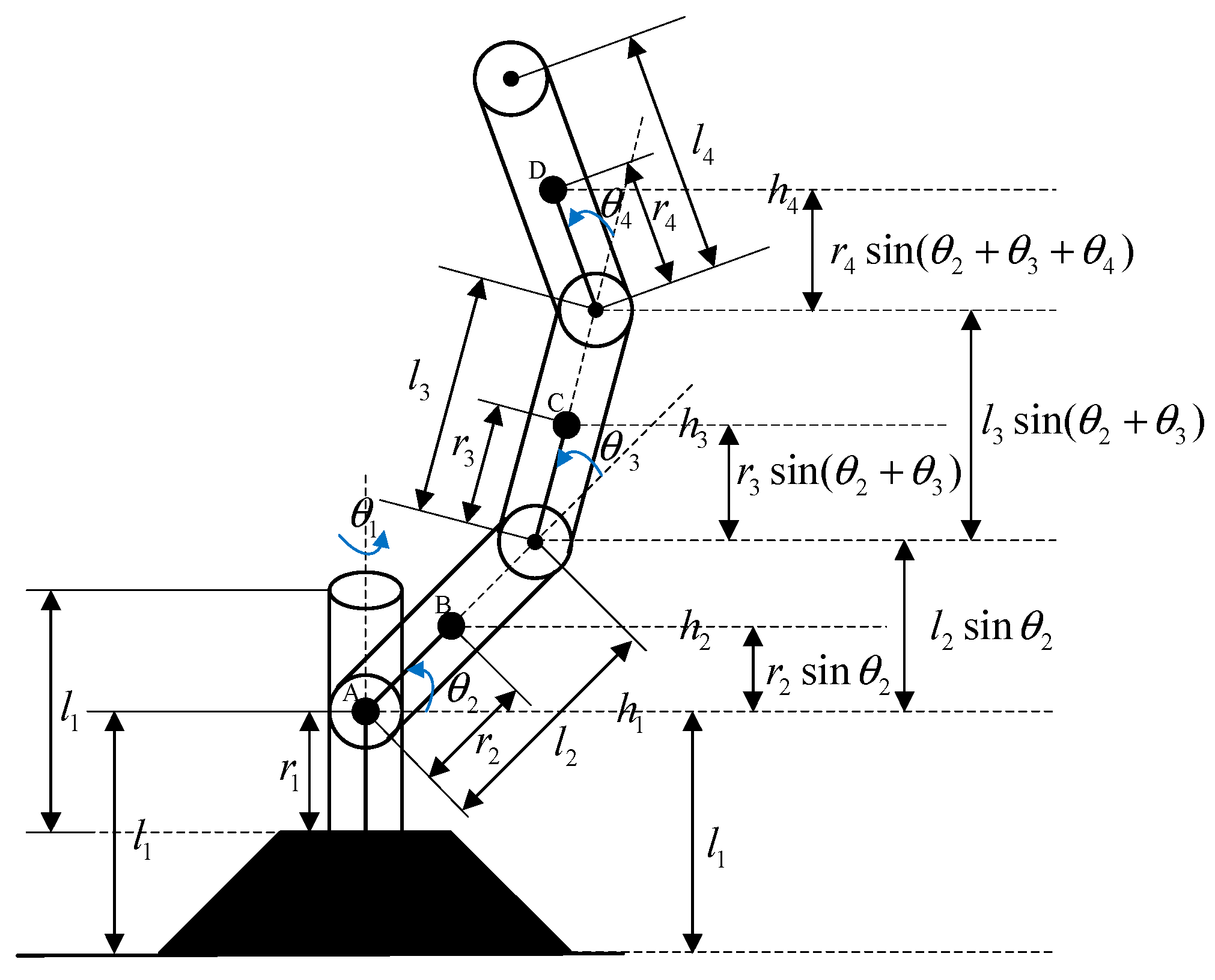
Figure 2.
The output trajectories for.
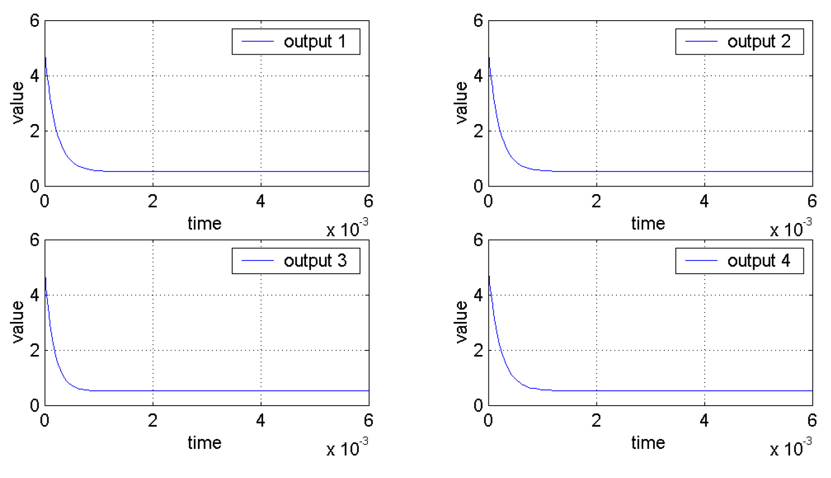
Figure 3.
The output trajectories for.
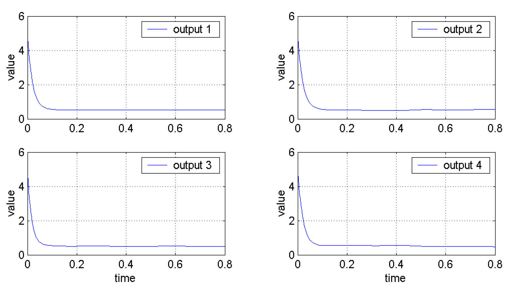
Figure 4.
Tracking error before entering the global final attractor.
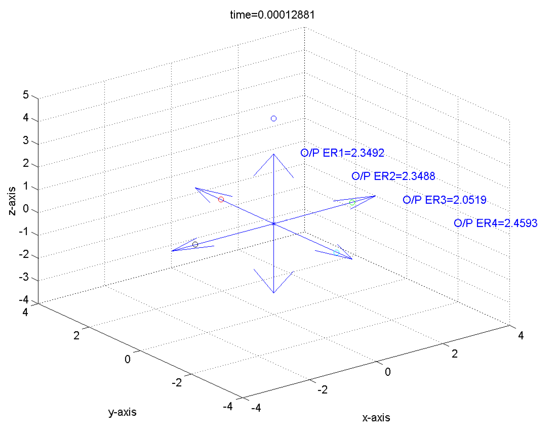
Figure 5.
Tracking error on entering the global final attractor.
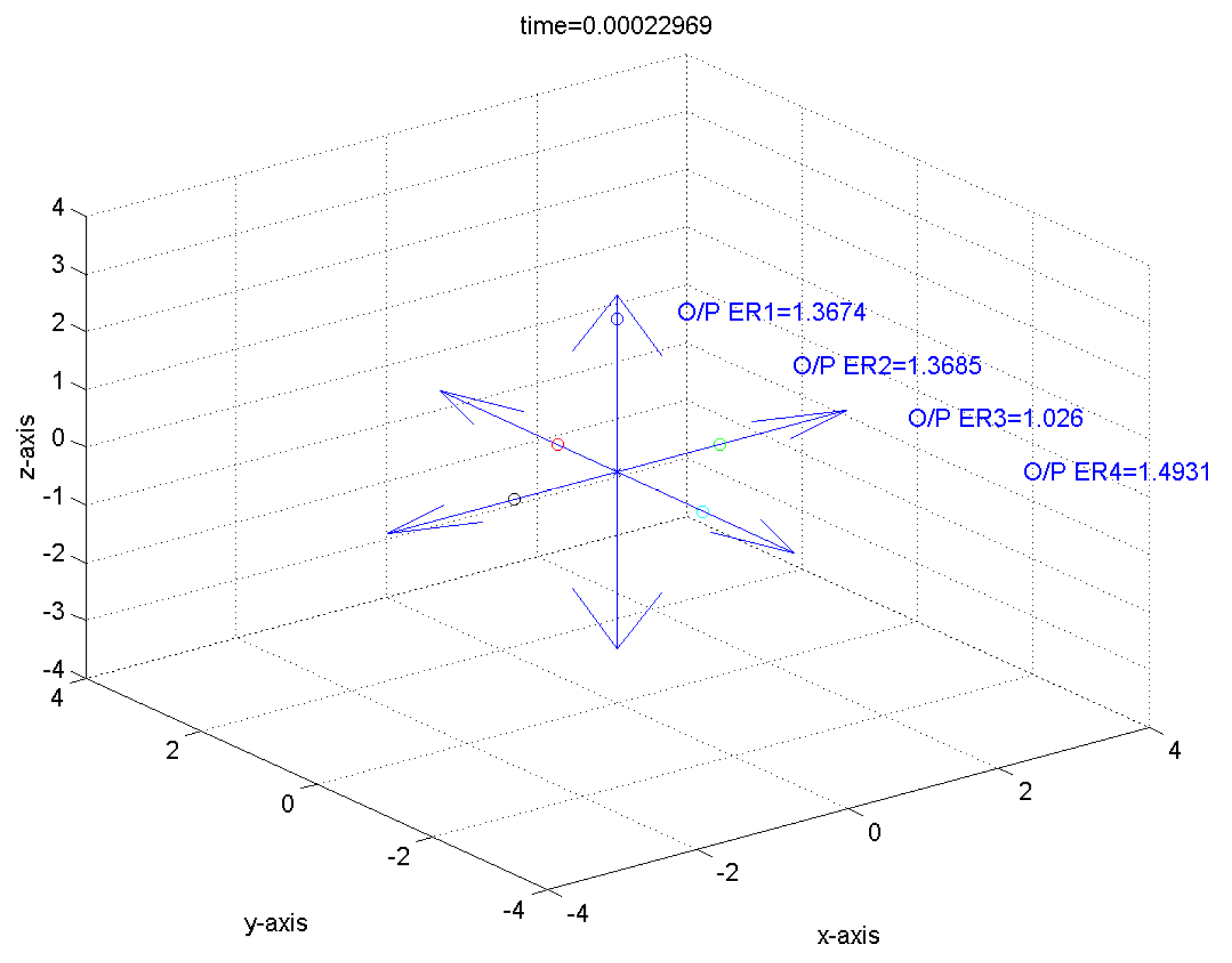
Figure 6.
Tracking error after entering the global final attractor.
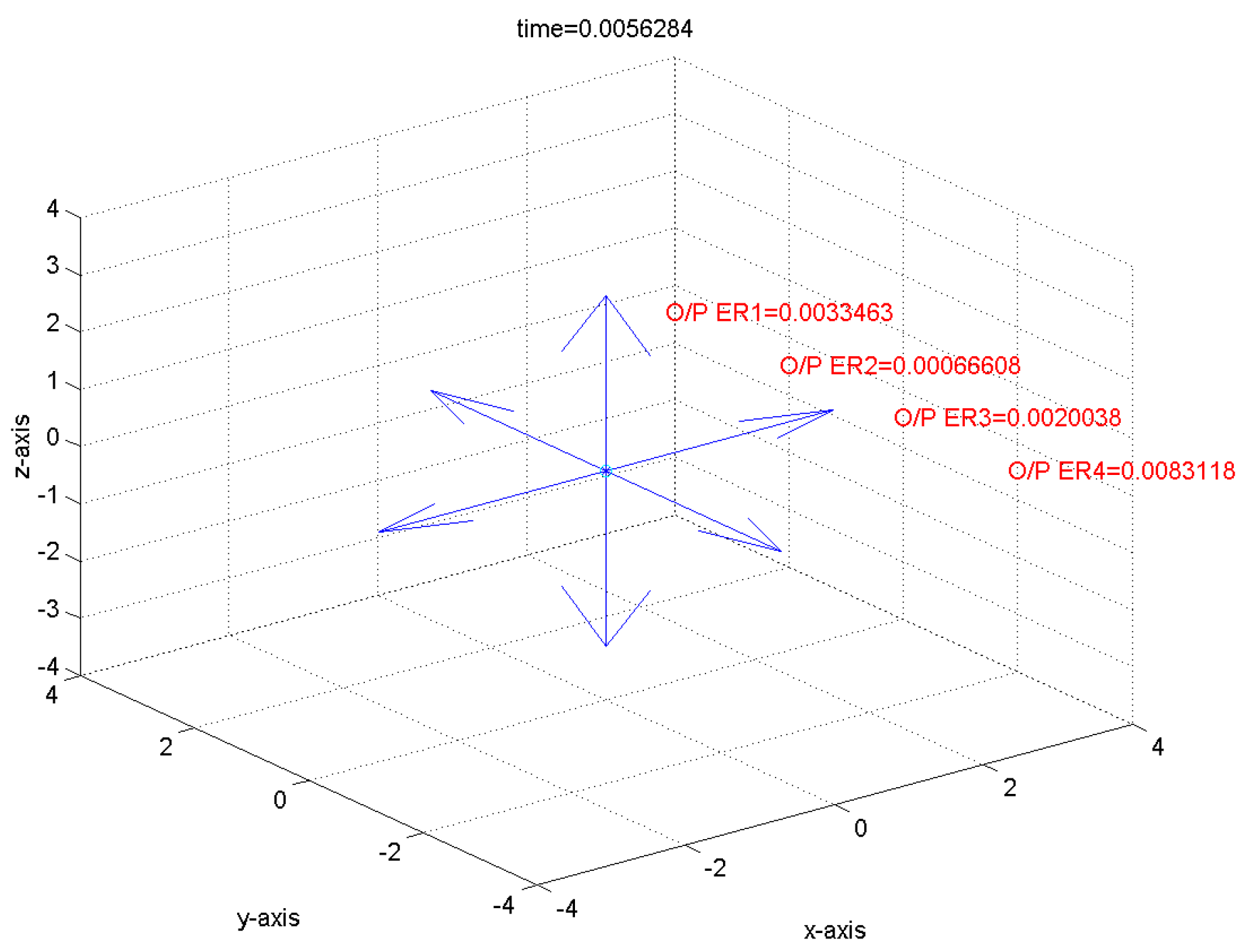
Figure 7.
General structure of traditional fuzzy approach.
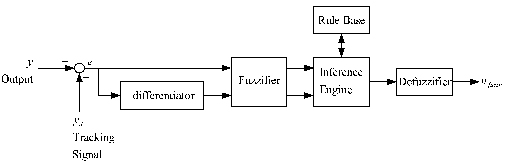
Figure 8.
Triangular shape membership functions for .

Figure 9.
Triangular shape membership functions for .
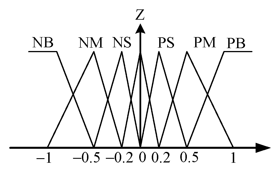
Figure 10.
Triangular shape membership functions for .
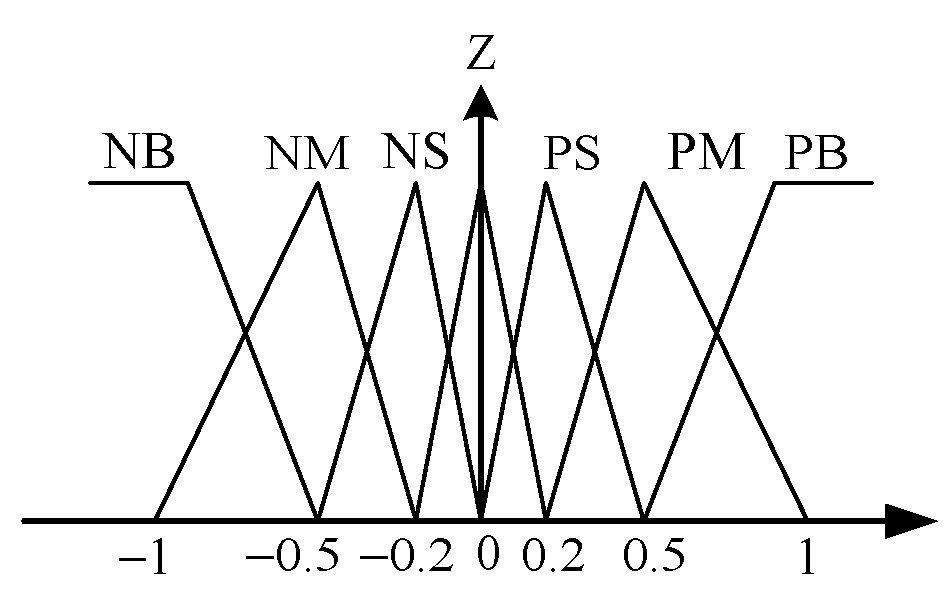
Figure 11.
The output tracking error for the output 1.
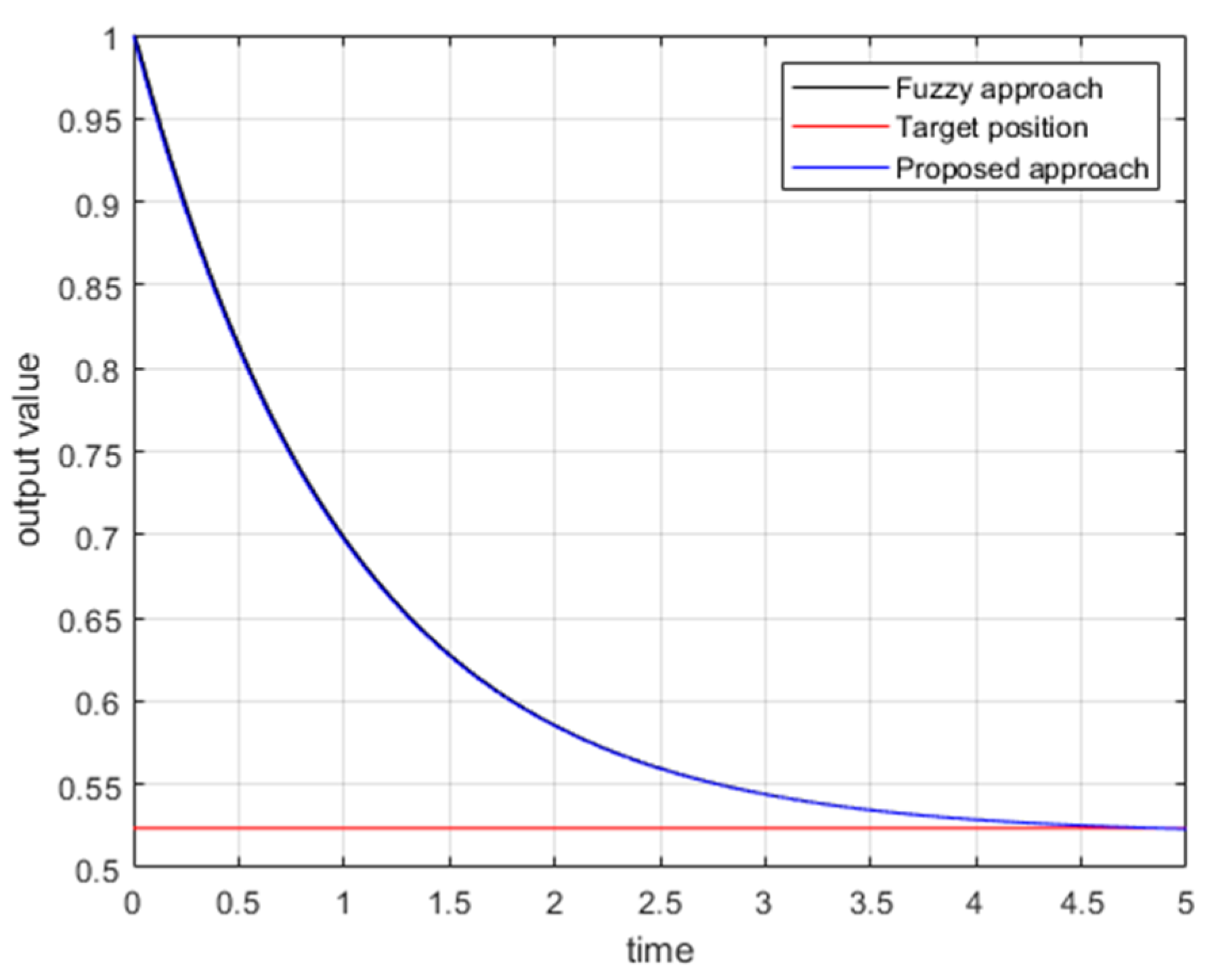
Figure 12.
The output tracking error for the output 2.
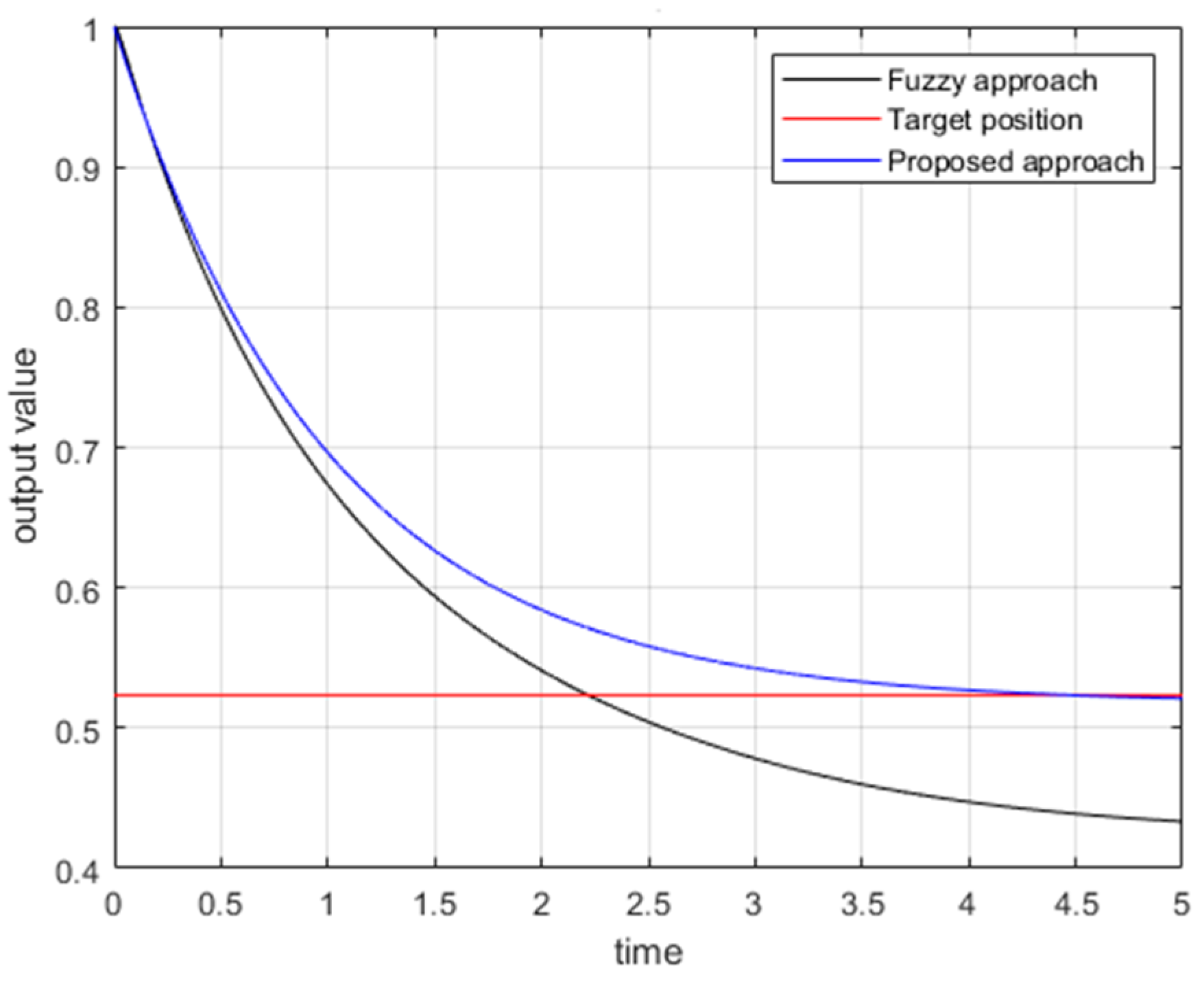
Figure 13.
The output tracking error for the output 3.
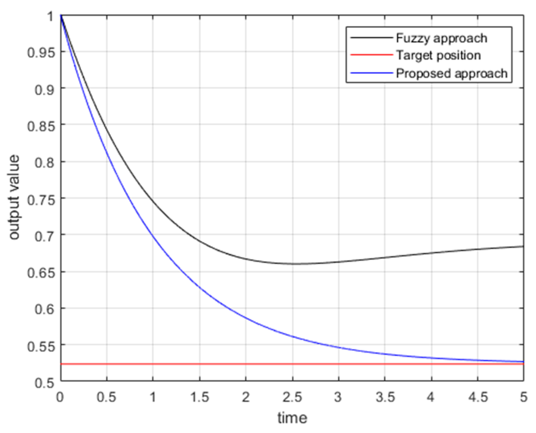
Figure 14.
The output tracking error for the output 4.
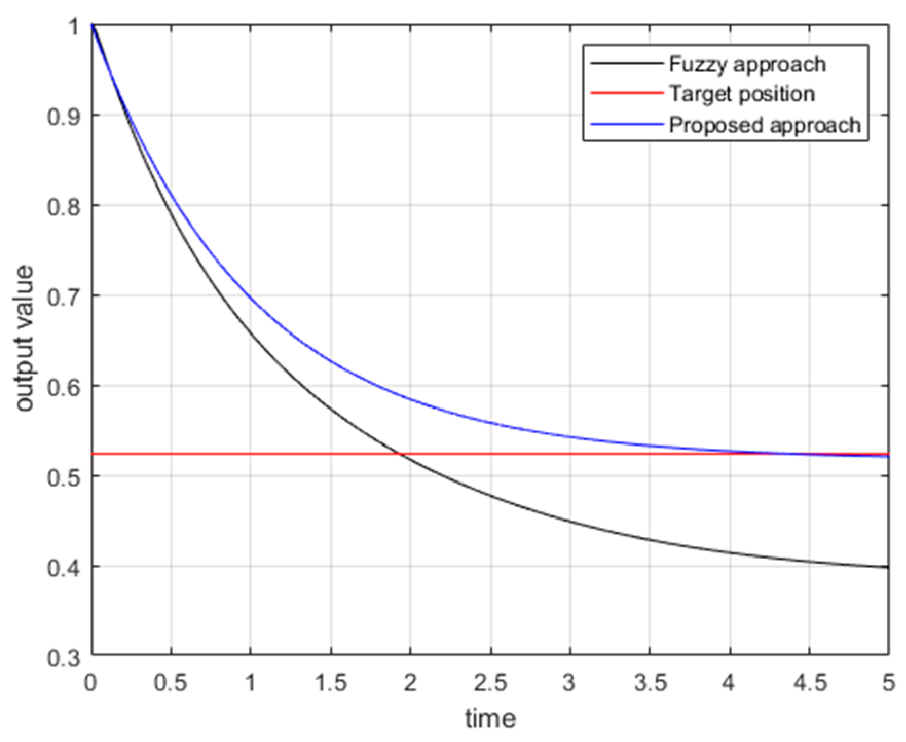
Figure 15.
The output trajectory of feedback-controlled system for (263).
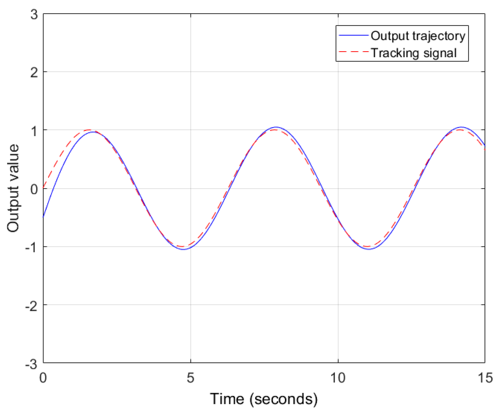

Table 1.
MACVICAR-WHELAN fuzzy control rule base.
| NB | NM | NS | ZE | PS | PM | PB | ||
| NB | PB | PB | PB | PB | PM | PS | ZE | |
| NM | PB | PB | PB | PM | PS | ZE | NS | |
| NS | PB | PB | PM | PS | ZE | NS | NM | |
| ZE | PB | PM | PS | ZE | NS | NM | NB | |
| PS | PM | PS | ZE | NS | NM | NB | NB | |
| PM | PS | ZE | NS | NM | NB | NB | NB | |
| PB | ZE | NS | NM | NB | NB | NB | NB | |
Disclaimer/Publisher’s Note: The statements, opinions and data contained in all publications are solely those of the individual author(s) and contributor(s) and not of MDPI and/or the editor(s). MDPI and/or the editor(s) disclaim responsibility for any injury to people or property resulting from any ideas, methods, instructions or products referred to in the content. |
© 2025 by the authors. Licensee MDPI, Basel, Switzerland. This article is an open access article distributed under the terms and conditions of the Creative Commons Attribution (CC BY) license (http://creativecommons.org/licenses/by/4.0/).
Copyright: This open access article is published under a Creative Commons CC BY 4.0 license, which permit the free download, distribution, and reuse, provided that the author and preprint are cited in any reuse.


