
Submitted:
21 February 2025
Posted:
24 February 2025
You are already at the latest version
Abstract
In various fields, planar 2R underactuated robot have garnered significant attention due to their numerous applications. To guarantee the stable control of these robots, a simple control strategy is presented in this paper, and we utilize the intelligent optimization algorithm to enhance the controller parameters. Initially, a comprehensive dynamic model is developed for the robot with its control properties described. Subsequently, we design a PD controller to control the movement of the planar 2R underactuated robot. Utilizing the differential evolution algorithm (DEA) with the considering the underactuated constraint to enhance the PD controller parameters to get the best control effect, which make all links reach the goal state. The findings from the simulation demonstrate the efficacy of the approach, and the designed strategy shows higher stability and convergence rate, highlighting its important contribution in the field of underactuated robots.
Keywords:
Planar underactuated robot
; differential evolution algorithm
; underactuated system
1. Introduction
Usually, the system with numerous inputs and degrees of freedom are common in everyday life. It is going to become an underactuated system when the quantity of control inputs of the original system is less than the system freedom number[1,2,3,4,5,6,7,8,9,10]. The benefits of an underactuated system include low weight, low cost, and low energy consumption. When some devices of the fully actuated system fail, the underactuated control method can improve reliability and ensure continuous operation. The underactuated robot is a typical system in underactuated system. The underactuated robots can be categorized into two cases based on whether or not they are affected by gravity: vertical underactuated robots [11,12,13] and planar underactuated robots[14,15,16]. This paper focuses on planar underactuated robots.
The planar underactuated robot have several potential applications in space research [17] and deep-sea exploration [18,19]. Since deep sea and space are microgravity or gravity free environments, robots have more advantages than humans in terms of operation and safety when performing some command operations. Therefore, rearching this type of system’s control method has enormous practical implications. The motion process of the planar robot is through the control method designed by our to make the robot arrive from any position in the plane to any position we need. According to the prior studies of planar underactuated robot, the linear approximation model is found to be uncontrollable in any equilibrium point during the control process. Therefore, the realization of this kind of robot position control is more complicated and difficult than other robot systems. As a matter of fact, the characteristics of control for the underactuated robot are closely related to the quantity of links and the passive joints position. With the location and quantity become different, the control characteristics will also change differently. Two different scenarios of planar underactuated robots, i.e., the holonomic system and the nonholonomic system, are also caused by their distinct properties[20,21].
The planar 2R underactuated robot is divided into two types, one is the planar Acrobot and the other is the planar Pendubot. The planar Acrobot is a planar 2R underactuated robot whose first joint is passive for it is fail or damaged. It possesses holonomic characteristics and a relationship defined by angular constraints. Lai [22] et al. deduced the angular constraint of link based on integrability, and achieved position control by regulating the active joint with the aid of the angle constraint. In [23], the good position control was achieved by using the method of model reduction and energy attenuation. In [24], for the planar Acrobot, a position strategy is proposes to control the robot from any starting position, the motion control of the planar Acrobot consists of two distinct phases, and under the coupling effect between the system states, the robot’s position control goal is realized. Planar Pendubot, an 2R underactuated robot whose second joint is passive, is a member of the nonholonomic system that is subject to an angular acceleration restriction [25]. It is challenging to intuitively determine the mathematical connection between these links which are active and passive due to the intricate nonlinear features of such systems. To accomplish stable control of the system, an open-loop iterative control approach was created by Luca [26] on account of the nilpotent approximation model. In addition, an innovative optimization technique based on Fourier transform was put forth in [27] to realize the stability control for planar Pendubot. The above is for planar Acrobot and planar Pendubot respectively carried out research, for their unified control methods, there are also some. In [28], the unified control of planar 2R underactuated robot is studied, and a control strategy that incorporates trajectory planning alongside tracking control is introduced, which successfully realizes the control objectives of the system. For 2R underactuated robots, Wang [29] proposes a trajectory planning tracking control strategy based on the basis function superposition method and intelligent optimization algorithm, and only relied on the second-order nonholonomic constraints commonly possessed by 2-DOF rotary underactuated robots to achieve unified control of such systems, simulation tests verified the efficacy of the strategy.
Based on the above analysis of previous studies, the research of planar 2R underactuated robot lays a foundation for the control theory research of underactuated robot. Currently, most previous studies only have proposed control methods for robots with specific structures and functions. Due to the uncertainty of passive joint position, it is necessary to explore a unified control strategy for both planar Acrobot and planar Pendubot in order to realize effective control of planar 2R underactuated robot. However, when a joint of a planar full actuated joint fails and becomes a passive joint, if the position of the passive joint cannot be directly determined, the present control methods are relatively simple and the control stability time is longer. Therefore, in order to realize the effective control of the planar 2R underactuated robot in this case, it is essential to investigate more simple and general method to realize the unified control strategy of the two robots above.
Therefore, this paper presents a simple planar 2R underactuated robot control strategy. By optimizing PD parameters, the controller is reformed to reduce the duration of stabilize to the desired state. The structure of the subsequent chapters of this paper is elaborated from the following aspects: A dynamic model of a planar 2R underactuated robot system is established in section 1.1, and the characteristics of the system are described in section 1.2. Then in section 2, a PD controller with adjustable parameters is designed. To attain the desired control objective, in section 3, the differential evolution algorithm (DEA) [30] is used to continuously enhance the parameters to obtain the optimal control effect, so as to ensure that each link can best achieve the control objective. Finally, in section 4, three sets of simulation experiments with different initial conditions and target conditions are carried out for the 2R underactuated robot Acrobot and Pendubot respectively to assess the efficacy and universal applicability of the method.
2. Model and Characteristics
This section is mainly to establish a planar 2R underactuated robot model and analyze its underactuated control characteristics, so as to pave the way for the subsequent controller design.
2.1. Model
The mechanical architecture of the planar 2R underactuated robot is shown in the Figure 1. is the angle of i-th(i=1, 2) link, is the mass of this link, and respectively are length of the link and the distance from the midpoint of the link to the center of the joint axis, and stands for the moment of inertia. is the applied torque at the i-th joint and r = 1, 2.
When an active joint of the planar robot fails or is damaged, the joint will lose its driving ability and become a passive joint, and the whole system will become an underactuated system. Moreover, due to the different positions of damaged or failed joints, the planar underactuated robot will exhibit different characteristics.
The object of this paper is the planar 2R underactuated robot, whose dynamic model is constructed as follows
In this model, is the vector of angle, is the angular velocity and is the angular acceleration of the planar robot. In the dynamic model, the contains the Coriolis and centrifugal forces and it belongs to . and expression in detail as follows in the whole dynamic model [31].
According to the position of the passive joint, the planar 2R underactuated robot can be categorized into two distinct scenarios:
Situation 1: the planar Acrobot, the passive joint is the first joint and torque vector is ,
Situation 2: the planar Pendubot, the passive joint is the second joint and torque vector is .
The following is the precise representation of every element in the matrix above:
where
2.2. Control Characteristic Analysis
The passive part of (1) is
where p = 1,2 except r, who indicates the p-th of the robot is a passive joint.
Equation shown below could be obtained by Equation (5) and the constraint relation of underactuated characteristics.
where the initial angle and angular velocity of the underactuated link are denoted by and , respectively. The Equation (6) specifically expresses that the underactuated link is constrained by the actuated link state.
3. Controller Design
We design a PD controller in this subsection in order to steer all links toward their desired states. And let the , in which represent , the angles of the two links of the robot and are , the angular acceleration at the two linking joints. Then following state space expression can be further obtained as
In this state space equation,
and
The active link’s control goal determines the selection of Lyapunov function, and it is shown in Equation (10).
where represents the positive constant, and ; represents the angular state of the link, represents the angular target state of the link, ; represents the angular velocity of the link, .
Then the derivative of is going to be
Therefore, the controller design of the system is as follows
where . The matrix is positive definite matrix, so is nonzero. Thus, it is possible to avoid the singular difficulties of the control torque .
It is obvious from Equation (13) that is bounded. Then define the following conditions
in which . Any solution x of Equation (15) coming from still remains in for all . By setting as the invariant of Equation (14), we get
Set , , then substitute it into Equation (7) and get the following result.
According to the LaSalle invariability principle [32], when the Equation (16) reaches the predetermined control goal, the state of the actuated link is , .
Therefore, when the following conditions are satisfied, the linkage of the planar 2R underactuated robot system is controlled to the target state.
Where, and are small positive error coefficient given.
Based on the above analysis, when the actuated link is stable to the desired state, the underactuated link is still rotating at a uniform speed. Therefore, this paper designs a simple PD controller for the actuated link, and optimizes the controller parameters through differential evolution algorithm. Through the controller, the underactuated link is also stabilized to the desired state.
4. Controller Parameter Optimization
The active link’s control objectives could be achieved by the intended controller, because the controller (12) forces the actuated link to remain stable at its goal position. Therefore, the DEA is used to calculate and respectively to guarantee that the unactuated link successfully attains its intended state.
The DEA’s evaluation function, as explained in [30].
where , and .
The following are the parameters of the designed controller calculated by DEA.
Process 1: Random initialization of and .
Process 3: If h is less than (a tiny positive constant), the optimization operation completed. The result of the promotion are and . If not, the program moves on to the next phase.
Process 4: Update and through mutation, crossover, and selection procedures by using (mutation factor) and (crossed factor). The procedure then turns to Process 2.
Based on the optimized controller parameters and , the link controller can be determined, and then the initial and target state parameters can be set to verify the designed controller by simulation.
5. Simulations
In this section, the proposed control strategy is verified by Matlab simulation, three sets of simulations are carried out on plane Acrobot and plane Pendubot for a planar 2R underactuated robot under different initial and target states, respectively, to assess the efficacy of the proposed control strategy. We choose the same length, weight and moment of inertia for both links. Table 1 shows the unified parameters of the planar 2R underactuated robot model.
5.1. The Simulation for Planar Acrobot
When the first link fails or is damaged, the planar 2R underactuated robot has underactuated characteristics. In this case, the main drive is the second link and torque is applied to link 2, i.e. . How to use the motion of the second actuated link to control the first link to stabilize to the target state is a problem that the simulation experiment must take into account. The model structure is transformed into a planar underactuated robot Acrobot. The converted Acrobot model is shown in Figure 2.
Therefore, we consider that we will first move the second link to the target state under the action of torque. At the same time, according to the above constraints of the planar Acrobot underactuated robot, under the action of PD controller, the appropriate parameters are optimized to control the first underactuated connecting rod to move to the target state, and finally realize the stability control of the whole planar Acrobot.
5.1.1. Simulation Result 1 for Planar Acrobot
The parameters of the differential evolution algorithm are selected as follows: maximum number of iterations =100, population number N=50, variation factor =0.3, crossover factor =0.7, = 0.005. Using DEA to controller parameters calculated and optimized Equation (12), so that it can attain optimal control efficacy on the planar Acrobot. The results of parameter optimization are as follows
The initial and target states of our chosen simulation 1 are shown in Equation (22).
Where , , , represent the starting angle and desired angle of the first link and the second link respectively, and , , , represent the initial angular velocity and target angular velocity of the two links respectively.
The control of planar Acrobot has achieved the target shown in the simulation results 1, and each state variable is primely convergent to the predetermined value.
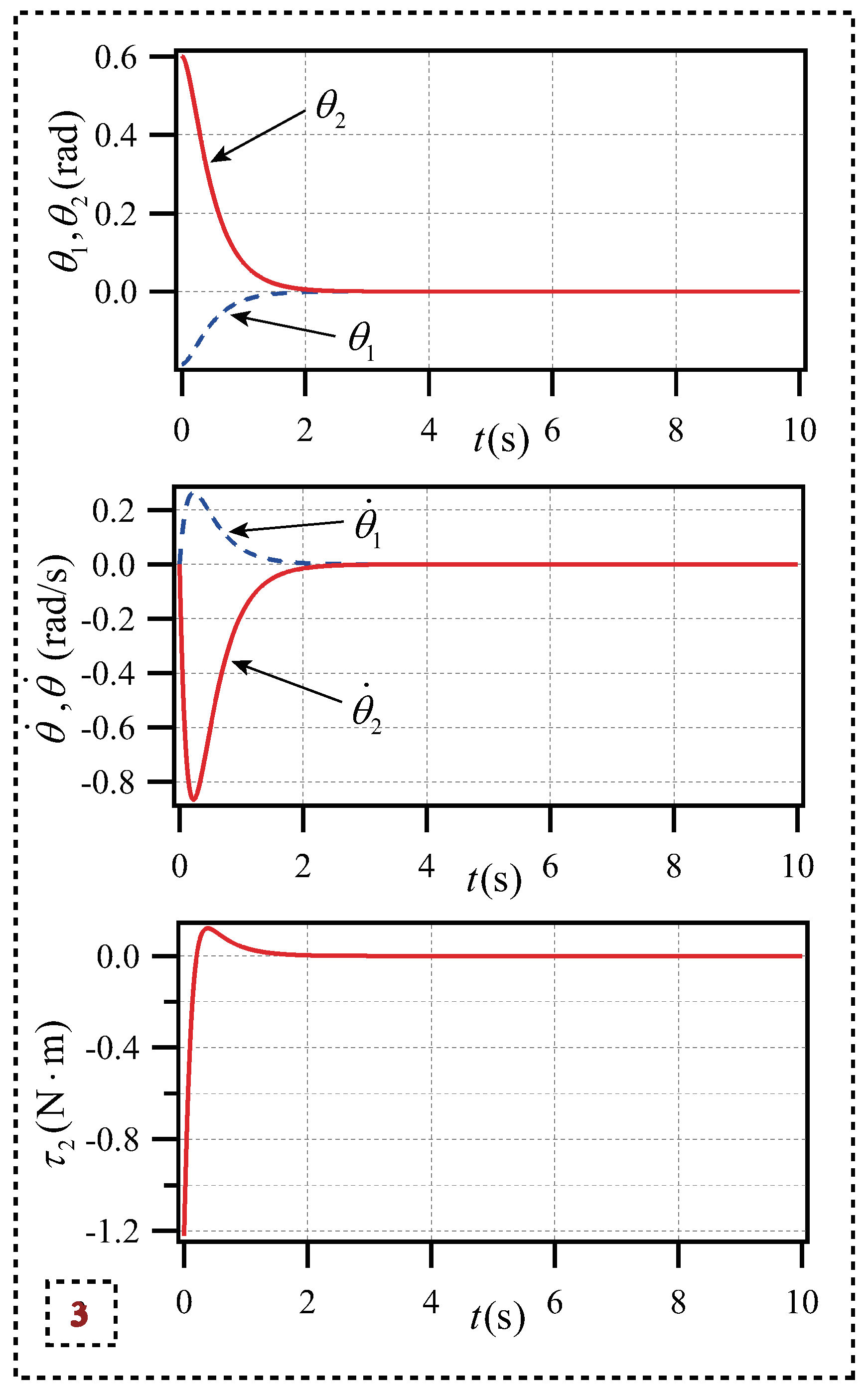
Figure 3 shows the each state variable changes of the two links of the planar Acrobot and the torque changes of the actuated link. As can be seen from the Figure 3, the planar Acrobot has reached the target state and remained stable before t = 5s, the maximum angular velocity does not exceed =15rad/s, and the torque range is maintained . To satisfy the system’s control requirements, the control strategy has good rapidity and system stability.
5.1.2. Simulation Result 2 for Planar Acrobot
Under the condition that the algorithm parameters remain unchanged, transform different starting condition and desired condition parameters to continue the optimization. The optimization parameters of the simulation result 2 are shown as follow.
In simulation result 2, the starting state and the desired state are
As shown in simulation result 2, the state variables of the two links of the planar Acrobot and the torque changes of the passive link change. The planar Acrobot before t = 4s to achieve the target state and maintain stability, the maximum absolute angular speed does not exceed =10rad/s, the value of the torque is still maintained in the range of , and to achieve planar Acrobot fast stability control requirements.
Figure 4.
Simulation result 2 for planar Acrobot.

Figure 5.
Simulation result 3 for planar Acrobot.
5.1.3. Simulation Result 3 for Planar Acrobot
To assess the validity of the suggested control strategy, set up a set of simulation, set state parameters, and optimize PD controller parameters by DEA. The parameters of simulation result 3 are
In the simulation 3, the starting and desired states of the planar Acrobot respectively are
The third set of simulation results has been presented. The final results indicate that the control method successfully converges to the target state within t=3s, the angular velocity range is rad/s, and the range of torque is maintained at . The control goal can still be achieved.
In simulation 2 and 3 of planar Acrobot, we set different parameters and different target states, but in the end it is ideal in terms of speed and stability. In addition, compared with the reference [28], this method is simpler and can control the target state quickly without the need of trajectory planning.
5.2. The Simulation for Planar Pendubot
When the second link of the planar 2R underactuated robot fails or is damaged, then the model has underactuated characteristics, and the model structure is transformed into the planar Pendubot underactuated robot. The specific structure is shown in Figure 6, and simulation experiments are carried out on the planar Pendubot model.
Also, three sets of different starting state parameters and desired state parameters are selected to carry out simulation on the planar Pendubot underactuated robot. For the planar Pendubot underactuated robot model, in this case the main driver is the first link and torque is applied to link . The first link moves to the target state under the action of torque. At the same time, according to the constraint relation of the planar Pendubot underactuated robot, the second underactuated link is controlled to move to the desired state, and the stability control of the entire planar Pendubot is finally realized.
5.2.1. Simulation Result 1 for Planar Pendubot
Similarly, the parameters of the differential evolution algorithm are selected as follows: maximum number of iterations =100, population number N=50, variation factor =0.3, crossover factor =0.7, = 0.005. Using DEA to controller parameters calculated and optimized Equation (12), so that it can attain optimal control efficacy on the planar Acrobot. The results of parameter optimization are as follows
In the simulation 4, the starting state and the desired state are
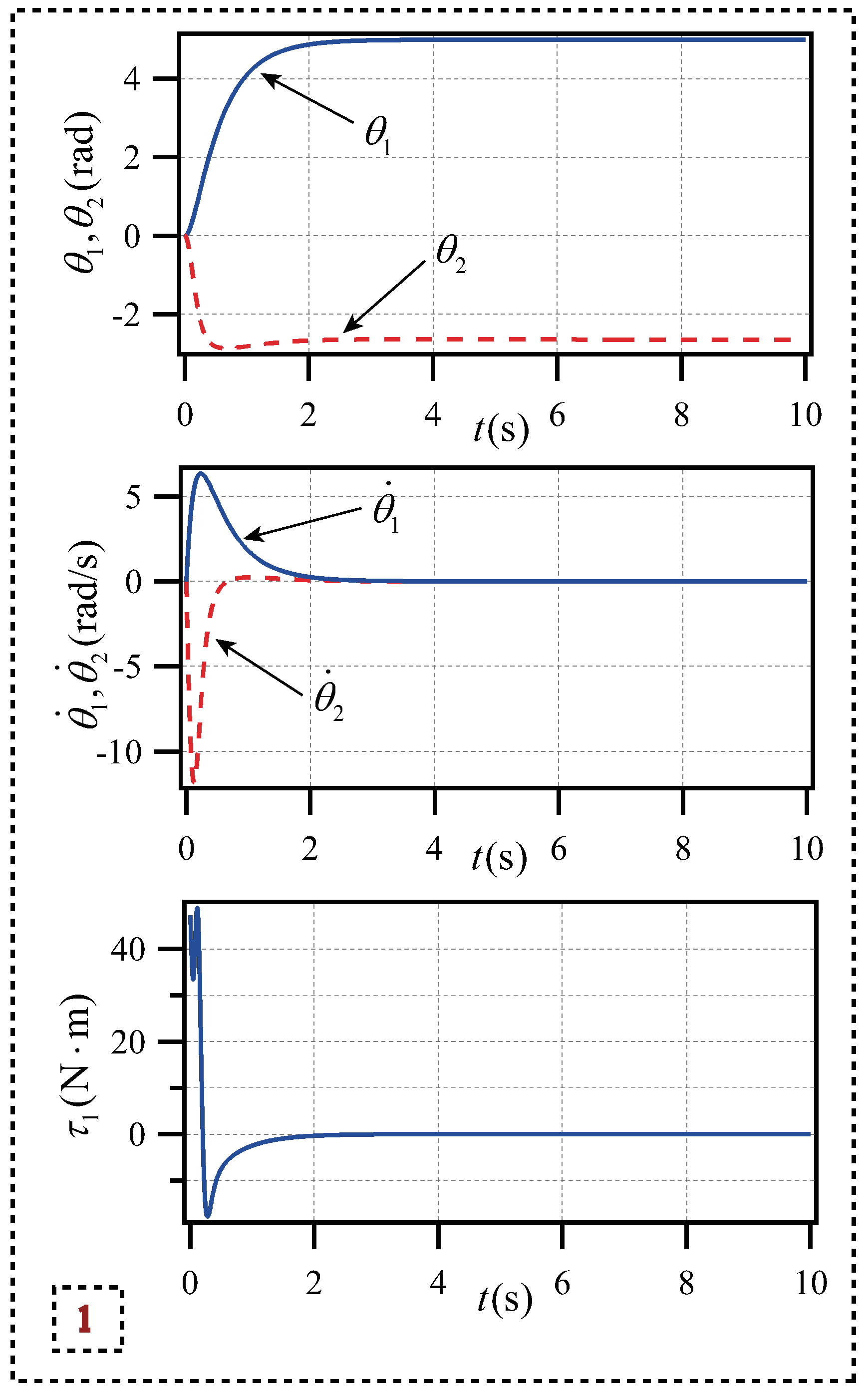
The control of planar Pendubot reaches the target shown in the simulation results 1, and each state variable basically converges to the predetermined value. Figure 9 shows the variation of each state variable of the planar Pendubot two-link mechanism and the torque variation of the movable link mechanism. Before t = 5s, the planar Pendubot has reached the target state and maintained stability. The angular velocity range is , and the control torque range is within , which meets the control requirements of the system. Therefore, this control strategy has good rapidity and system stability for planar Pendubot.
5.2.2. Simulation Result 2 for Planar Pendubot
In the same case that the algorithm parameters are unchanged, different starting state parameters and desired state parameters are transformed to continue the optimization. Optimization parameters of simulation result 2 are as follows:
In simulation result 2, the starting state and the desired state are
The planar pendubot control achieves the target shown in the simulation results 2, and each state variable basically converges to the predetermined value. Under the second set of state parameters, the changes of state variables of the planar penddubot double-connecting rod mechanism and the changes of torque of the movable connecting rod mechanism are analyzed. Before t= 4s, the planar penddubot has reached the target state and remains stable. The angular velocity range is , and the control torque range is within , which reachs the control goal of the system.
Figure 7.
Simulation result 2 for planar Pendubot.
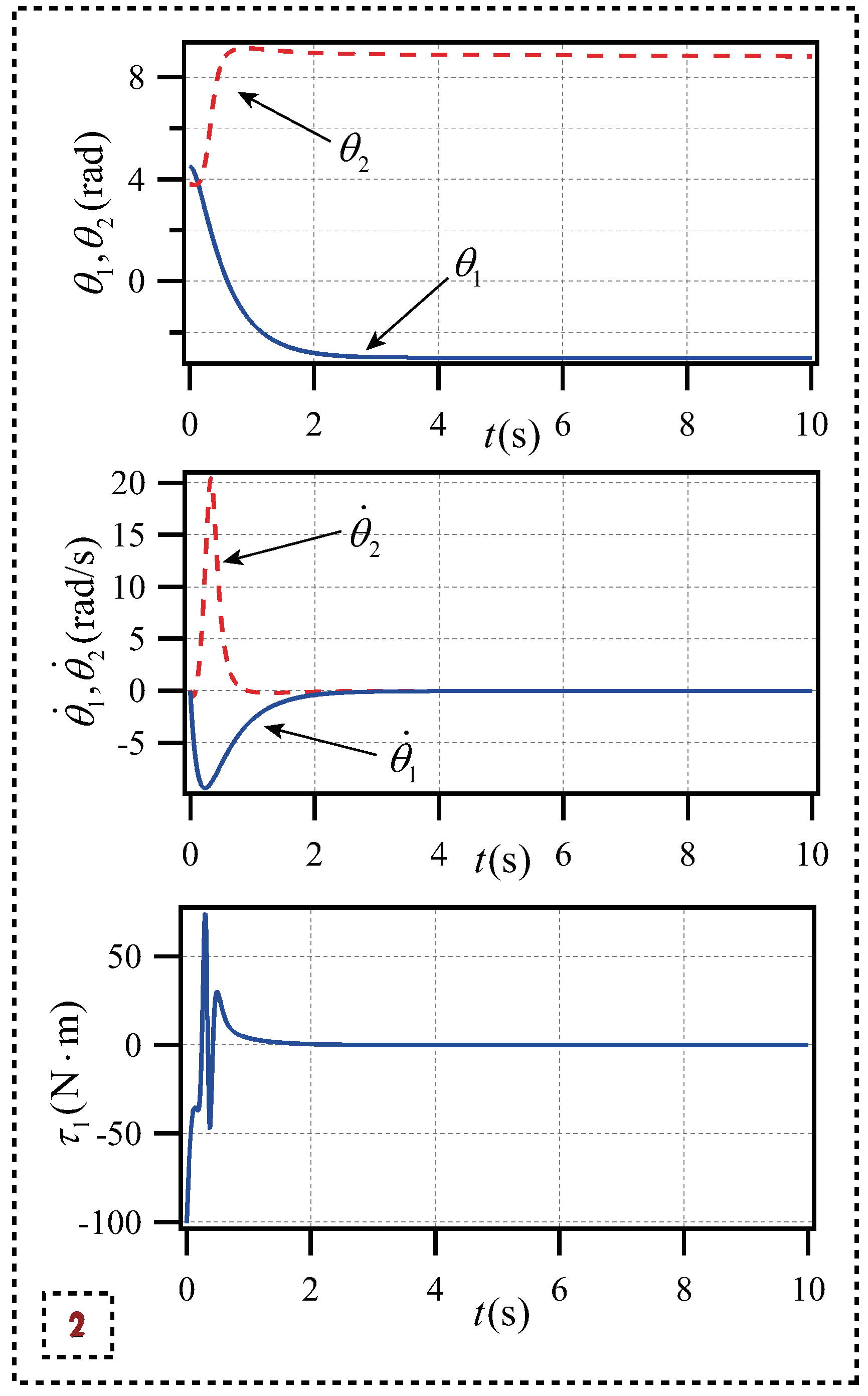
Figure 8.
Simulation result 3 for planar Pendubot.
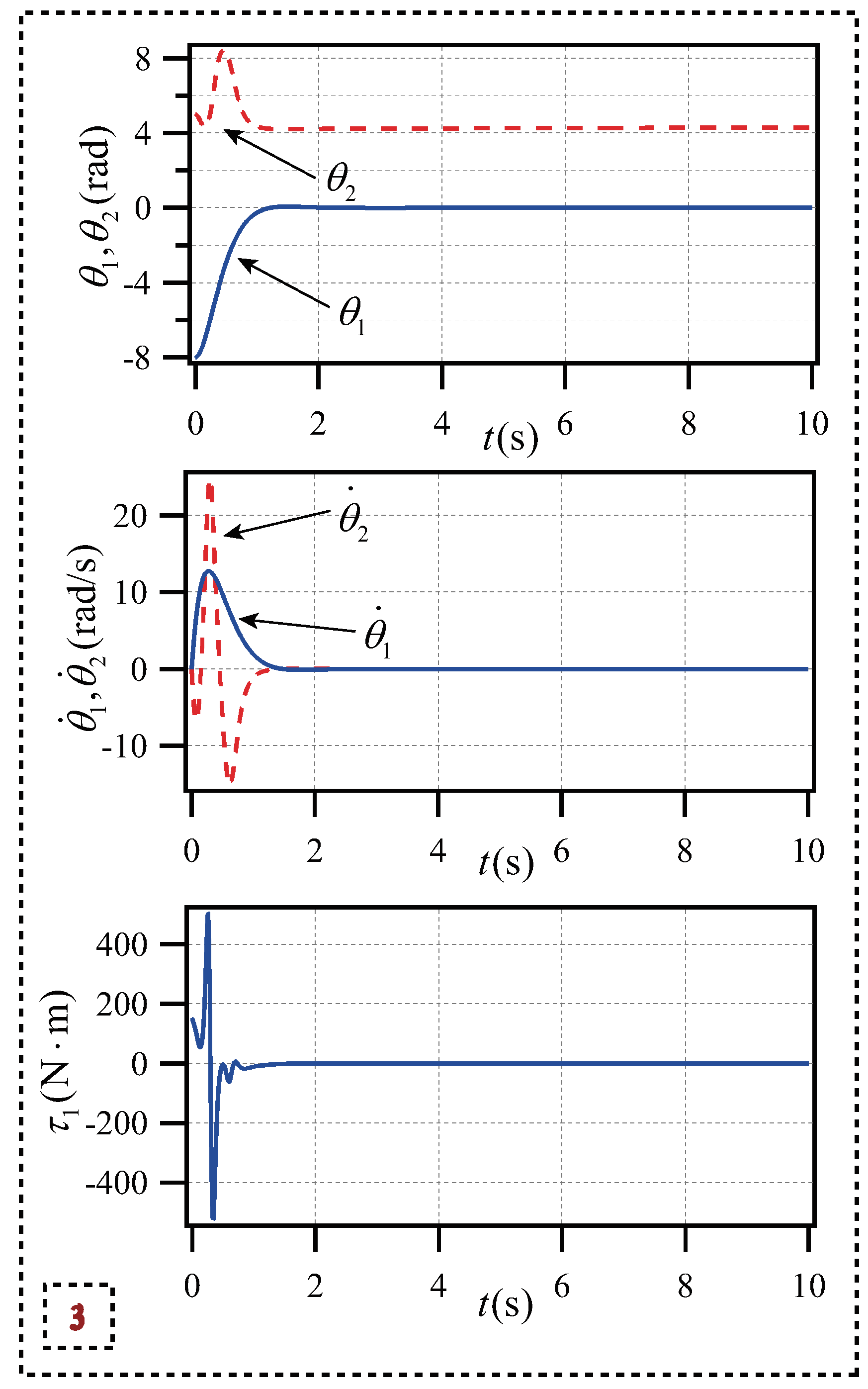
Figure 9.
Simulation result 1 for planar Pendubot.
5.2.3. Simulation Result 3 for Planar Pendubot
To confirm the general applicability of the strategy to the planar Pendubot underactuated robot, the third set of simulation experiments was conducted, and the following state parameters were selected to optimize the PD controller by differential evolution algorithm. The parameters of simulation result 3 are
In simulation result 3, the initial and target states of each state variable of the planar Pendubot respectively are
Under the third set of state parameters, the planar penddubot control reaches the target shown in the simulation results, and each state variable basically converges to the predetermined value. Before t= 3s, the planar penddubot has reached the target state and remains stable. The angular velocity range is , and the control torque range is within .
In the simulation 2 and 3 of planar Pendubot, different parameters and different target states are set, and the simulation results indicate that the results are good in terms of speed and stability. In addition, compared with the reference [28], this method is simpler and can control the target state quickly without the need of trajectory planning.
5.3. Analysis of Simulation Results
For planar Arcobot and planar Pendubot underactuated robots, three groups of different state parameters were selected to design a simple PD controller, and the parameters of PD controller were successfully optimized by differential evolution algorithm. The proposed control strategy’s effectiveness was validated through simulation. The following are three different groups of parameter indicators in the control process of planar Arcobot and planar Pendubot underactuated robots, as shown in Table 2 and Table 3.
The results of Table 2 and Table 3 show that the rotation angle of all the links in the simulation successfully converges, and the stable control of the target state is achieved. The maximum time does not exceed 5s, and the change of angular velocity is proportional to the change of torque, which proves the validity and universal applicability of the control strategy.
6. Conclusions
A simple PD control strategy is proposed for planar 2R underactuated robot. The suitable controller parameters are obtained by DEA method. After this, the PD controller is determined to enable the entire system to transition from its starting state to the target state under the action of the actuated linkage. Finally, the validity and general applicability of the proposed strategy are verified by simulation, and the potential relationship between the change of angular velocity and the magnitude of torque is found. In summary, compared with other methods, a relatively simple control strategy is proposed, which can realize fast and stable control without trajectory planning. In addition, the method can be easily applied to other underactuated robots.
In future work, we will develop this simple and effective control method to deal with underactuated robots with more degrees of freedom, swarm underactuated robot control and underactuated robots with multiple passive joints. This control method expands the whole method library of nonlinear control and underactuated control, and provides theoretical basis and design ideas for subsequent research.
Author Contributions
Planning research programmes and making comments, Z.H; Collect data for simulation and paper writing, X.G; Model building and literature collection, X.W; Provide technical support and advice, H.Z.
Funding
This research was funded by the Nature Science Foundation of Hubei Province (No. 2023AFB380), the Hubei Key Laboratory of Digital Textile Equipment (Wuhan Textile University) (No. KDTL2022003), the Hubei Key Laboratory of Intelligent Robot (Wuhan Institute of Technology) (No. HBIRL202301).
Institutional Review Board Statement
Not applicable.
Informed Consent Statement
Not applicable.
Data Availability Statement
The data presented in this study are available on request from the corresponding author.
Conflicts of Interest
The authors declare no conflicts of interest.
References
- Lu, B.; Fang, Y.C. Online trajectory planning control for a class of underactuated mechanical systems. IEEE Trans. Autom. 2024, 69, 442–448. [Google Scholar] [CrossRef]
- Zhang, K. K; Zhou,B.; Jiang, H.; Duan, G.R. Finite-time control of a class of nonlinear underactuated systems with application to underactuated axisymmetric spacecraft. IEEE Trans. Aerosp. Electron. Syst. 2023, 59, 7061–7071. [Google Scholar]
- Harandi, M.R.J.; Khalilpour, S.A.; Taghirad, H.D. Adaptive energy shaping control of a 3-DOF underactuated cable-driven parallel robot. IEEE Trans. Industr. Inform. 2023, 19, 7552–7560. [Google Scholar] [CrossRef]
- Han, F.; Yi, J.G. Stable learning-based tracking control of underactuated balance robots. IEEE Rob. Autom. 2021, 6, 1543–1550. [Google Scholar] [CrossRef]
- Fu, Y.; Sun, N.; Yang, T.; Qiu, Z.H.; Fang, Y.C. Adaptive coupling anti-swing tracking control of underactuated dual boom crane systems. IEEE Trans. Syst., Man, Cybern. 2022, 52, 4697–4709. [Google Scholar] [CrossRef]
- Pucci, D.; Romano, F.; Nori, F. Collocated adaptive control of underactuated mechanical systems. IEEE Trans. Robot. 2015, 31, 1527–1536. [Google Scholar] [CrossRef]
- Yang, T.; Sun, N.; Fang, Y.C. Adaptive fuzzy control for a class of MIMO underactuated systems with plant uncertainties and actuator dead zones: design and experiments. IEEE Trans. Cybern. 2022, 52, 8213–8226. [Google Scholar] [CrossRef]
- Huang, Z.X.; Lai, X.Z.; Zhang, P.; Meng, Q.X.; Wu, M. A general control strategy for planar 3-DoF underactuated manipulators with one passive joint. Inform. sciences. 2020, 534, 139–153. [Google Scholar] [CrossRef]
- Xu, F.; Wang, H.H.; Liu, Z.; Chen, W.D. Adaptive visual servoing for an underwater soft robot considering refraction effects. IEEE Trans. Ind. Electron. 2020, 67, 10575–10586. [Google Scholar] [CrossRef]
- Lu, B.; Fang, Y.C. Online trajectory planning control for a class of underactuated mechanical systems. IEEE Trans. Automat. Contr. 2024, 69, 442–448. [Google Scholar] [CrossRef]
- Wang, L.J.; Lai, X.Z.; Meng, Q.X.; Wu, M. Effective control method based on trajectory optimization for three-link vertical underactuated manipulators with only one active joint. IEEE Trans. Cybern. 2023, 53, 3782–3793. [Google Scholar] [CrossRef] [PubMed]
- Zou, Y.; Zhou, Z.Q.; Dong, X.W.; Meng, Z.Y. Distributed formation control for multiple vertical takeoff and landing UAVs with switching topologies. IEEE/ASME Trans. Mech. 2018, 23, 1750–1761. [Google Scholar] [CrossRef]
- Wang, L.J.; Lai, X.Z.; Zhang, P.; Wu, M. A control strategy based on trajectory planning and optimization for two-link underactuated manipulators in vertical plane. IEEE Trans. Syst., Man, Cybern. 2022, 52, 3466–3475. [Google Scholar] [CrossRef]
- Li, D.W.; Wei, Z.A.; Huang, Z.X. Two-stage control strategy based on motion planning for planar prismatic–rotational underactuated robot. Actuators. 2024, 13, 278–290. [Google Scholar] [CrossRef]
- Wang, Y.W.; Lai, X.Z.; Zhang, P.; Wu, M. Control strategy based on model reduction and online intelligent calculation for planar n-link underactuated manipulators. IEEE Trans. Syst., Man, Cybern. 2017, 50, 1046–1054. [Google Scholar] [CrossRef]
- Li, J.; Wang, L.J.; Chen, Z.; Huang, Z.X. Drift suppression control based on online intelligent optimization for planar underactuated manipulator with passive middle joint. IEEE Access. 2021, 9, 38611–38619. [Google Scholar] [CrossRef]
- Ma, Z.Q.; Huang, P.F.; Lin, Y.X. Learning-based sliding-mode control for underactuated deployment of tethered space robot with limited input. IEEE Trans. Aerosp. Electron. Syst. 2022, 58, 2026–2038. [Google Scholar] [CrossRef]
- Wang, K.; Liu, Y.H.; Li, L.Y. Vision-based tracking control of underactuated water surface robots without direct position measurement. IEEE Trans. Contr. Syst. Technol. 2015, 23, 2391–2399. [Google Scholar] [CrossRef]
- Wang, J.S.; Wang, J.; Han, Q.L. Receding-horizon trajectory planning for under-actuated autonomous vehicles based on collaborative neurodynamic optimization. IEEE/CAA J. Automatic. 2022, 9, 1909–1923. [Google Scholar] [CrossRef]
- Oriolo, G.; Nakamura, Y. Control of mechanical systems with second-order nonholonomic constraints: underactuated manipulators. Proc. IEEE Conf. Decis. Control 1991, 2398–2403. [Google Scholar]
- Wang, Z.Y.; Xin, X.; Liu, Y.N. Strong stabilization of two-link underactuated planar robots. 2022 China Automat. Congr. Xiamen, China, 2022; 4125–4129. [Google Scholar]
- Lai, X.Z.; She, J.H.; Cao, W.H.; Yang, S.X. Stabilization of underactuated planar acrobot based on motionstate constraints. Int. J. Non. Linear Mech. 2015, 77, 342–347. [Google Scholar] [CrossRef]
- Xiong, P.Y.; Feng, G.F.; Zeng, H.F.; Pan, C.Z. Position control for a planar underactuated manipulator based on model reduction and energy attenuation. 2022 Chin. Control Conf. Hefei, China, 2022; 884–889. [Google Scholar]
- Luo, Y.B.; Lai, X.Z.; Wu, M. A positioning control strategy of planar Acrobot. Proc. Chin. Control Conf. Yantai, China, 2011; 743–747. [Google Scholar]
- Shoji, T.; Katsumata, S.; Nakaura, S.; Sampei, M. Throwing motion control of the springed Pendubot. IEEE Trans. Control Syst. Technol. 2013, 21, 950–957. [Google Scholar] [CrossRef]
- Luca, A.D.; Mattone, R.; Oriolo, G. Stabilization of an underactuated planar 2R manipulator. Int. J. Robust Nonlinear Control. 2000, 10, 181–198. [Google Scholar] [CrossRef]
- Urrea, C.; Kern, J.; Alvarez, E. Design of ageneralized dynamic model and a trajectory control and position strategy for n-link under actuated revolute planar robots. Control Eng. Pract. 2022, 128, 5316–5329. [Google Scholar]
- Huang, Z.X.; Hou, M.Y.; Wei, S.Q.; Wang, L.J. The unified control strategy for planar Acrobot and Pendubot. J. Shenzhen Univ. Sci. Eng. 2023, 40, 275–283. [Google Scholar]
- Wang, H.N.; Hua, Y.; Chen, L. Unified control strategy of 2-DOF rotary underactuated manipulator. Modular Mach. Tool Automatic Manuf. Techn. 2024, 11, 152–155. [Google Scholar]
- Opara, K.P.; Arabas, J. Differential evolution: a survey of theoretical analyses. Swarm and Evol. Comput. 2019, 44, 546–558. [Google Scholar]
- Cao, S.Q.; Lai, X.Z.; Wu, M. Motion control method of planar Acrobot based on trajectory characteristics. Proc. Chin. Control Conf. Hefei, China 2012, 4910–4915. [Google Scholar]
- LaSalle, J.P. Stability theory for ordinary differential equations. J. Differ. Equ. 1968, 4, 57–65. [Google Scholar]
Figure 1.
Model of a planar 2R underactuated robot.
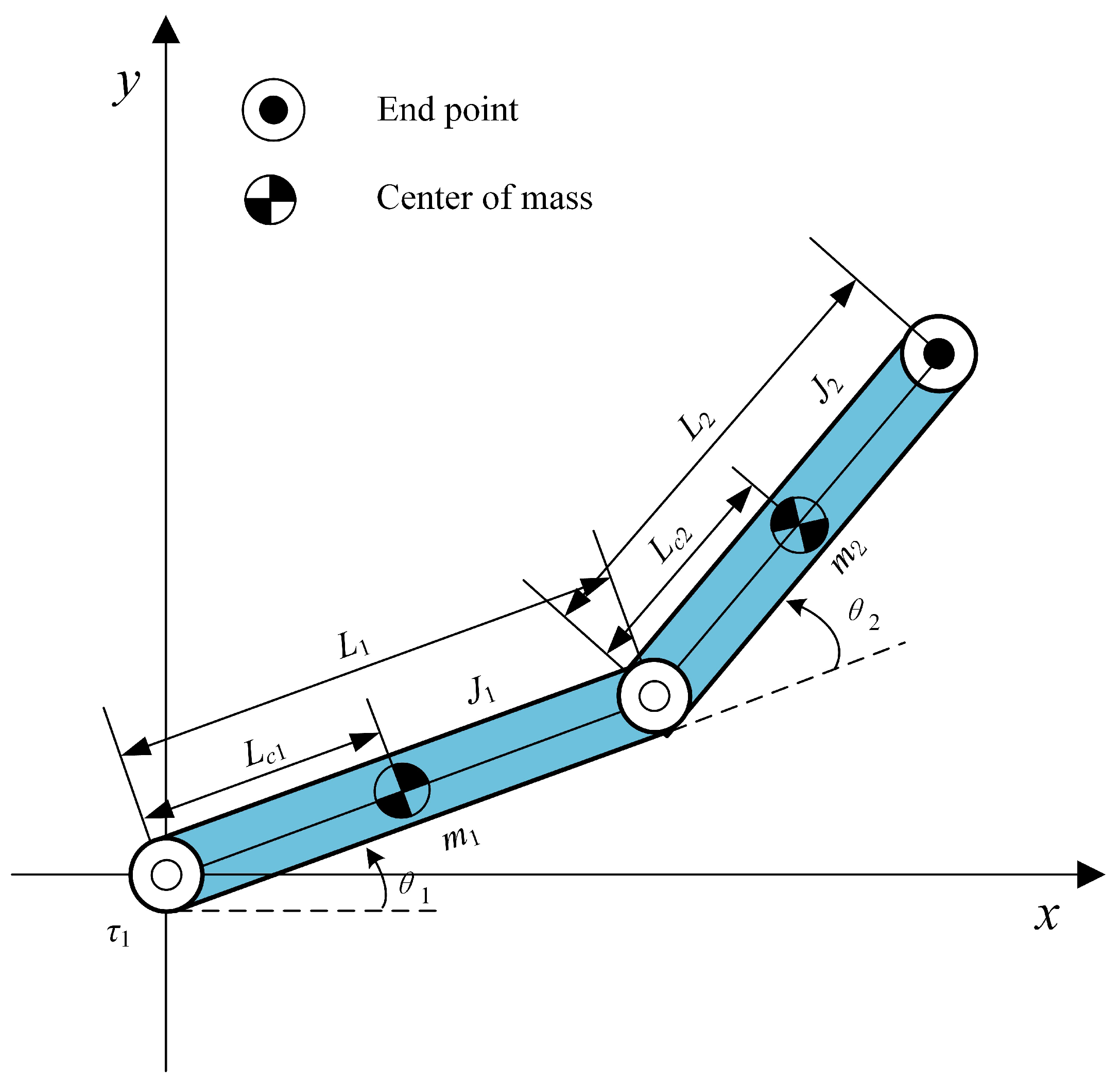
Figure 2.
The model of the planar Acrobot.
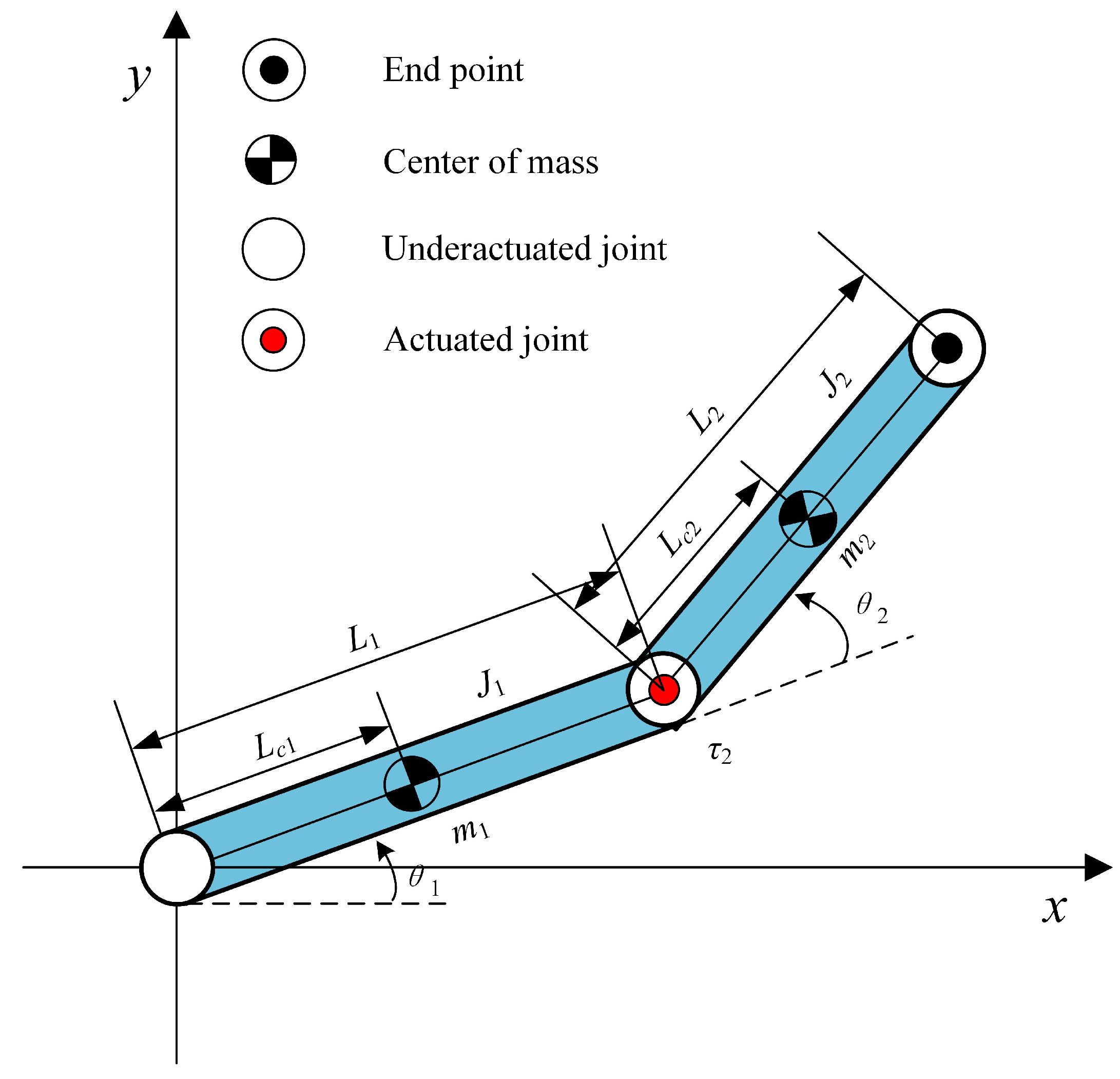
Figure 3.
Simulation result 1 for planar Acrobot.
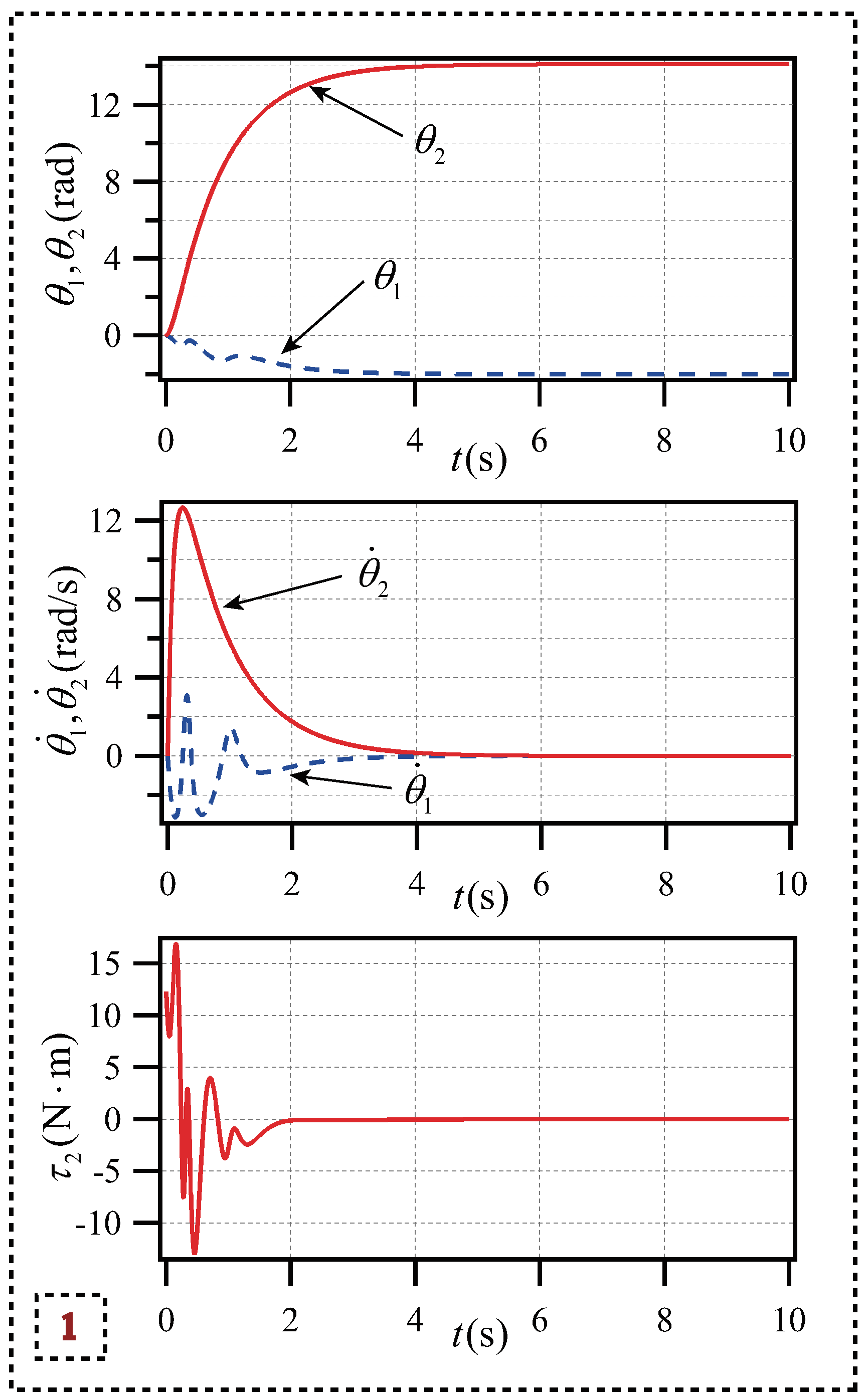
Figure 6.
The model of the planar Pendubot.


Table 1.
Planar 2R underactuated robot model parameters.
| Link i | ||||
|---|---|---|---|---|
| 1 | 1.0 | 0.5 | 1.0 | 0.0833 |
| 2 | 1.0 | 0.5 | 1.0 | 0.0833 |
Table 2.
Comparison of three simulation groups of planar Arcobot.
| Group i experiment | Convergence case | Stable time | Angular velocity range | Torque range |
|---|---|---|---|---|
| 1 | Success | Within 5s | ||
| 2 | Success | Within 4s | ||
| 3 | Success | Within 3s |
Table 3.
Comparison of three simulation groups of planar Pendubot.
| Group i experiment | Convergence case | Stable time | Angular velocity range | Torque range |
|---|---|---|---|---|
| 1 | Success | Within 5s | ||
| 2 | Success | Within 4s | ||
| 3 | Success | Within 3s |
Disclaimer/Publisher’s Note: The statements, opinions and data contained in all publications are solely those of the individual author(s) and contributor(s) and not of MDPI and/or the editor(s). MDPI and/or the editor(s) disclaim responsibility for any injury to people or property resulting from any ideas, methods, instructions or products referred to in the content. |
© 2025 by the authors. Licensee MDPI, Basel, Switzerland. This article is an open access article distributed under the terms and conditions of the Creative Commons Attribution (CC BY) license (http://creativecommons.org/licenses/by/4.0/).
Copyright: This open access article is published under a Creative Commons CC BY 4.0 license, which permit the free download, distribution, and reuse, provided that the author and preprint are cited in any reuse.


