Submitted:
24 March 2025
Posted:
25 March 2025
You are already at the latest version
Abstract
The airfoil optimization of vertical axis wind turbine (VAWT) often encounters challenges such as high computational costs and long convergence times, especially in the analysis of complex aerodynamic characteristics. When using the Computational Fluid Dynamics (CFD) method for optimization design, the computational workload is usually enormous, making it difficult to efficiently handle many design variables and complex aerodynamic parameters. In this paper, a design configuration with three blades, a chord length of 0.42 m, and a rotation radius of 1.4 m is adopted as the basis for optimization using the surrogate model. Subsequently, an optimization design is carried out through the proposed Kriging surrogate model in combination with the Multi - Island Genetic Algorithm (MIGA). The Kriging surrogate method for airfoil optimization significantly enhances the aerodynamic performance of the wind turbine. Particularly at high tip - speed ratios, its power coefficient is increased by 14.2%, which validates the effectiveness of this method in the optimization design of wind turbines. Meanwhile, this optimization strategy improves the aerodynamic performance of VAWT, enabling them to achieve better energy conversion efficiency under a wider range of operating conditions.
Keywords:
H-type VAWT
; MIGA
; Airfoil Optimization
; Kriging Surrogate Model
1. Introduction
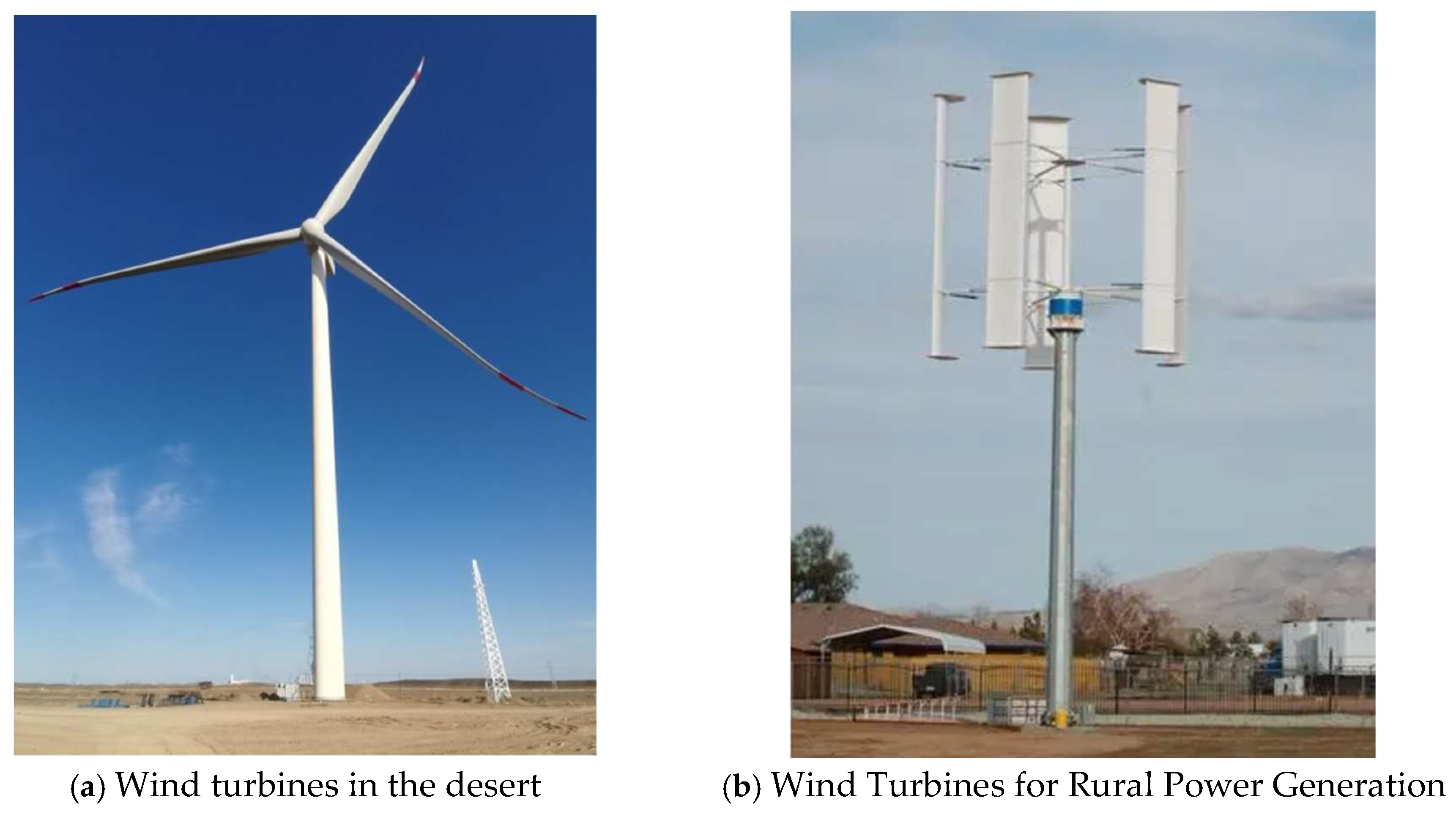
In recent years, vertical axis wind turbine (VAWT) have emerged as a research hotspot in the wind energy field due to their advantages of compact structure, omnidirectional wind capture capability, and low maintenance costs. Although this type of turbine demonstrates significant potential in distributed energy systems and complex terrain scenarios, its aerodynamic performance and power generation efficiency still face multiple technical challenges. Existing studies mainly focus on key issues such as airfoil parameter optimization, aerodynamic load fluctuation suppression, and low-wind-speed start-up performance improvement, among which airfoil design exerts a particularly significant impact on the overall performance of VAWT[1-2]. Traditional design methods encounter a long-standing technical bottleneck where it is difficult to balance start-up performance and high efficiency operating conditions, leading to chronically limited aerodynamic efficiency[3]. Additionally, while computational fluid dynamics (CFD) simulations can accurately analyze flow field characteristics, their high computational costs—with a single operating condition simulation taking over 72 hours—make them impractical for multi-parameter optimization requirements[4-5]. To address these issues, this paper proposes an optimization strategy based on the Kriging surrogate model. By constructing a collaborative optimization framework integrating high-fidelity surrogate modeling and the multi-island genetic algorithm, this approach achieves significant improvements in VAWT airfoil aerodynamics and validates the optimization effect on power generation efficiency across a wide range of operating conditions.
In recent years, scholars worldwide have conducted systematic research on the aerodynamic performance and power generation characteristics of VAWT. Zhu et al. [6] analyzed the evolution law of power generation performance of straight-bladed VAWT under variable wind speed and attack angle conditions using CFD methods. Mohammed et al. [7] systematically reviewed the aerodynamic design methodologies for VAWTs and compared the applicability of numerical simulation, wind tunnel experiments, and field tests as evaluation tools. Martino et al.[8] employed parametric modeling to reveal the influence mechanism of airfoil camber and thickness distribution on the power coefficient of VAWTs. Deshmukh [9] comprehensively reviewed the development history of VAWT and established an aerodynamic performance evaluation system for different types of airfoils. Haitian et al.[10] quantified the influence of turbulence intensity on aerodynamic loads and power curves of VAWT through a combined CFD-wind tunnel validation method. Shah et al. [11] proposed a collaborative optimization framework for blade shape, wind farm layout, and control strategy. Halawa [12] innovatively conducted experimental research on aerodynamic performance under turbulent wind conditions. Mohammed et al. [13] developed a dynamic load suppression technology based on variable-pitch control. Reyes et al. [14] established a power coefficient calculation model considering dynamic stall effects. Hand[15] clarified the coupling effect of blade geometric parameters and operating parameters through orthogonal experimental design. Notably, breakthroughs have been achieved in the application of artificial intelligence technology in the optimization of VAWT [16-20]. However, existing research still faces two technical bottlenecks: (1) traditional CFD simulations take over 72 hours per operating condition, making them unsuitable for multi-objective optimization requirements; (2) collaborative optimization research on the wide wind speed adaptability and turbulence robustness of airfoil aerodynamic design remains insufficient.
Figure 1.
Typical applications for different types of wind turbines.
To address the issues of high computational costs and long convergence cycles inherent in traditional CFD methods for vertical axis wind turbine (VAWT) airfoil optimization, this paper proposes an efficient optimization strategy based on the Kriging surrogate model. This approach establishes a collaborative optimization framework integrating parametric modeling, surrogate modeling, and the MIGA. By taking airfoil camber, thickness distribution, and twist angle as design variables, setting maximum relative thickness constraints, and formulating an optimization model with the full tip-speed ratio power extraction coefficient as the objective function, the method achieves global optimization of airfoil aerodynamic parameters through dynamic adjustments of population size and crossover/mutation probabilities. The optimization results demonstrate that the improved airfoil achieves an average 9.8% increase in power coefficient across a wide tip-speed ratio range, verifying the engineering practicality of this method in balancing computational efficiency and optimization accuracy. This study provides quantifiable theoretical foundations and technical pathways for VAWT airfoil design.
2. Theory of Optimal Design of H-type VAWT
2.1. Airfoil Parameters
The airfoil refers to the cross - sectional shape of a wind turbine blade, which determines the lift, drag, and power generated by the wind turbine when it operates in the wind. In the design of wind turbines, the selection and design of the airfoil are directly related to the performance and energy conversion efficiency of the wind turbine. The airfoils of wind turbine blades generally adopt curved shapes, such as the common dome airfoil and NACA airfoil. The design of these airfoils fully takes into account the flow characteristics of the wind and the functional requirements of the blades, aiming to achieve the best aerodynamic performance. As shown in Figure 2, it is a typical airfoil. The geometric parameters of the airfoil are the parameters used to describe the shape of the airfoil, mainly including the following [21].
The aerodynamic parameters of an airfoil include the drag, lift, and moment it generates. According to Bernoulli's principle and von Kármán vortex street theory, when airflow passes over the airfoil's upper surface, the flow velocity increases significantly, creating a velocity differential relative to the lower surface. This velocity gradient results in reduced static pressure on the upper surface and increased static pressure on the lower surface, thereby generating an upward lift force perpendicular to the incoming flow direction. Meanwhile, frictional effects on the airfoil surface and pressure differences caused by flow separation together form the drag force, while uneven distribution of aerodynamic forces produces a moment around the airfoil's axis of rotation. A schematic diagram of the aerodynamic forces acting on the airfoil is shown in Figure 3.
Drag, lift and moment are related to the size and shape of the airfoil, so they are generally expressed as dimensionless coefficients, which are drag coefficient , lift coefficient and pitching moment coefficient , which are defined as follows:
In the formula, is the air density, is the incoming wind velocity,c is the airfoil chord length,L、D、M denote the lift, drag, and pitching moment exerted on the airfoil, respectively.
2.2. H-VAWT Aerodynamic Change Law
As shown in Figure 4, the aerodynamic force F acting on the blade airfoil is composed of the lift force and drag force . The resultant vector can be decomposed into a tangential component and a normal component relative to the airfoil surface. Based on the aerodynamic parameter calculation model established in formulas (4) and (5), the lift and drag distributions on the airfoil surface can be accurately solved.
Based on the force analysis of a single blade airfoil, the torque of a single blade of a wind turbine in operating condition is calculated as follows:
This paper focuses on the study of the three-bladed H-VAWT, and the phase difference between the positional arrangements of each blade of the three-bladed H-VAWT is 120°. Therefore, the aerodynamic torque of each blade can be calculated by only determining the angle of attack of each blade, blade azimuth, tip speed ratio and relative wind speed. As follows:
Therefore, the torque and power of the wind turbine at a given instant can be deduced:
In the formula, and are the wind turbine torque coefficient and wind energy utilization factor, respectively.
Figure 5 illustrates the aerodynamic force distribution on the blades of an H-type vertical axis wind turbine (H-VAWT) at different azimuth angles. When the azimuth angle falls within the 0°–180° range, the angle of attack becomes negative, and the resultant vector of lift and drag forces points toward the rotor interior. Conversely, when the azimuth angle is in the 180°–360° range, the angle of attack turns positive, and the resultant vector points outward from the rotor. Notably, at 0° and 180° azimuth positions, only the drag component contributes to torque generation, and when the tip-speed ratio (TSR) exceeds 1, the torque becomes negative, with no contribution from the lift component. For other azimuth angles, torque arises from the combined action of lift and drag forces. Consequently, the overall loading state of the rotor represents the dynamic superposition of aerodynamic contributions from all blades. As the blades rotate, they alternately experience positive and negative angles of attack, thereby continuously providing driving torque to the rotor throughout the operational cycle.
3. Theoretical Methods
3.1. Computational Fluid Dynamics
Computational Fluid Dynamics (CFD) serves as a core tool for solving complex fluid mechanics problems through the integration of numerical methods and computer technology. Its underlying principle involves three key steps: first, discretizing the continuous fluid domain into a finite number of cells or grids, converting continuous physical quantities into discrete values at grid nodes; second, applying mathematical discretization techniques (such as the finite volume method or finite element method) to transform partial differential governing equations describing fluid motion (e.g., the Navier-Stokes equations) into systems of algebraic equations; and finally, using iterative solution algorithms (e.g., the SIMPLE algorithm) to obtain nodal values of physical quantities such as velocity, pressure, and temperature in the flow field [22].
The basic governing equations of CFD are the N-S equations of hydrodynamics, and the three-dimensional N-S equations are as follows:
In the formula, is a conserved variable,, , are convective fluxes, , , are viscous fluxes, denoted respectively:
Turbulence is a ubiquitous complex nonlinear phenomenon in fluid flow, characterized by random velocity fluctuations, generation and evolution of vortex structures, and chaotic streamline motion. The role of turbulence modeling in CFD is to simulate and predict turbulence phenomena in fluid flow, and the accuracy of turbulence simulation directly affects the results of CFD calculations. The k-ω SST turbulence model, which is most used in the field of rotating machinery, can accurately capture the flow separation and re-attachment phenomena during mechanical rotation with the following formulation:
In this paper, the k-ω SST turbulence model, which is widely recognized in the field of rotating machinery, is adopted. This model can accurately capture the nonlinear characteristics of fluid motion with its excellent computational accuracy, especially in the simulation of rotationally induced flow separation and reattachment phenomena and is suitable for high-fidelity numerical simulations under complex flow field conditions.
3.2. Airfoil Optimization Methods
This paper employs the Classification and Shape Transformation (CST) parametrization method to construct airfoil geometric models. This approach enables accurate reconstruction of airfoil profiles using a parsimonious set of design variables, with parameters possessing clear geometric interpretations. The CST parametrization process involves the following key steps [23]:
The expression for the classification function C(x) is as follows:
In the formula, x is the normalized airfoil chord length, which takes the value of [0,1], k is the scale factor, N1, N2 are the shape parameters, and for the rounded-head and blunt-tailed airfoils, k=1,N1=0.5,N2=1。
Define the shape function S(x) in terms of Bernstein polynomials, specifically:
In the formula, is the coefficient factor, the expression is shown in equation (2-36), is the coefficient to be found, and n is the order.
With the shape function S(x) and the classification function C(x), the expression for the airfoil profile is obtained by superimposing the airfoil thickness ∆z after the expression:
In the formula, and are the parameters that control the airfoil curve substitution.
For the airfoil optimization of H-VAWT, the NACA 0015 airfoil is selected as the initial reference profile. The optimization parameter system consists of 13 design variables: 12 cubic Bernstein polynomial coefficients for defining the upper/lower surface geometry of the airfoil, and 1 blade setting angle for adjusting the blade's angular orientation relative to the rotational plane. The NACA0015 airfoil fitting results are shown in Figure 8, which shows a good fit to the original data.
3.3. Design of Airfoil Optimization Model
A. Agent model
The Kriging surrogate model employed in this study traces its origins to the geostatistical interpolation method developed in 1951. Over six decades of evolution, this model has emerged as a powerful tool for modeling complex nonlinear systems, notably effective even with limited sample sizes. The surrogate model construction process involves three critical phases: (a) Select a certain number of sample points through the experimental design method; (b) Calculate the value of the objective function of the extracted sample points; (c) Train the agent model using the sample points and the objective function and verify its accuracy. The construction process of Kriging model is described in detail below.
The Kriging agent model predicts the distribution of function values at unknown points by calculating the predicted mean and variance of the function at the target point, which is widely used because of its very good nonlinearity and goodness of fit compared to other agent models [77], and the basic Kriging equations are as follows.
In the formula, g(x) is called deterministic drift and is a non-random part, generally polynomial; while z(x) is called rise and fall and is characterized as follows:
The Kriging model requires that the prediction variance of the model is minimized, and ultimately the Kriging model expression for the output of the system can be obtained by derivation as follows:
In the formula,
The commonly used kernel function used in this paper is the exponential function:
With the sample points known, the values , vectors , g(x), and vectors r(x) can be determined by regression analysis and kernel function calculations to obtain the response equations for the Kriging model.
B. H-VAWT computational model
To validate the accuracy of numerical calculations, this study establishes a benchmark verification model for an H-VAWT based on the Musgrove P wind tunnel experiment [81]. The model employs NACA 0015 airfoils with a blade chord length of 0.4 m, configured in a three-blade symmetrical layout. The rotor radius is 1.25 m, the blade pitch angle is fixed at 0°, and the blade-hub connection point is located at 0.15 chord lengths from the leading edge. The incoming wind speed is 10m/s, the rotational speed is 4rad/s~24rad/s, and its blade distribution is shown in Figure 9, which is taken as the starting position of the wind turbine calculation.
According to the wind tunnel model used in the test, the computational model is divided into three computational domains, as shown in Figure 10, A represents the fixed domain of the rotor axis and the outflow field, B represents the rotational domain of the blade, and the data of numerical computation are transferred between different domains by means of the intersection interface, in which the rotor axis has a radius of 0.5 m, the rotational domain has a radius of 2.8 m, the inlet adopts 10 times the rotational radius, the outlet adopts 32 times the rotational radius, and the upper and lower boundaries use 12 times the rotation radius to establish the outflow field.
C. Meshing
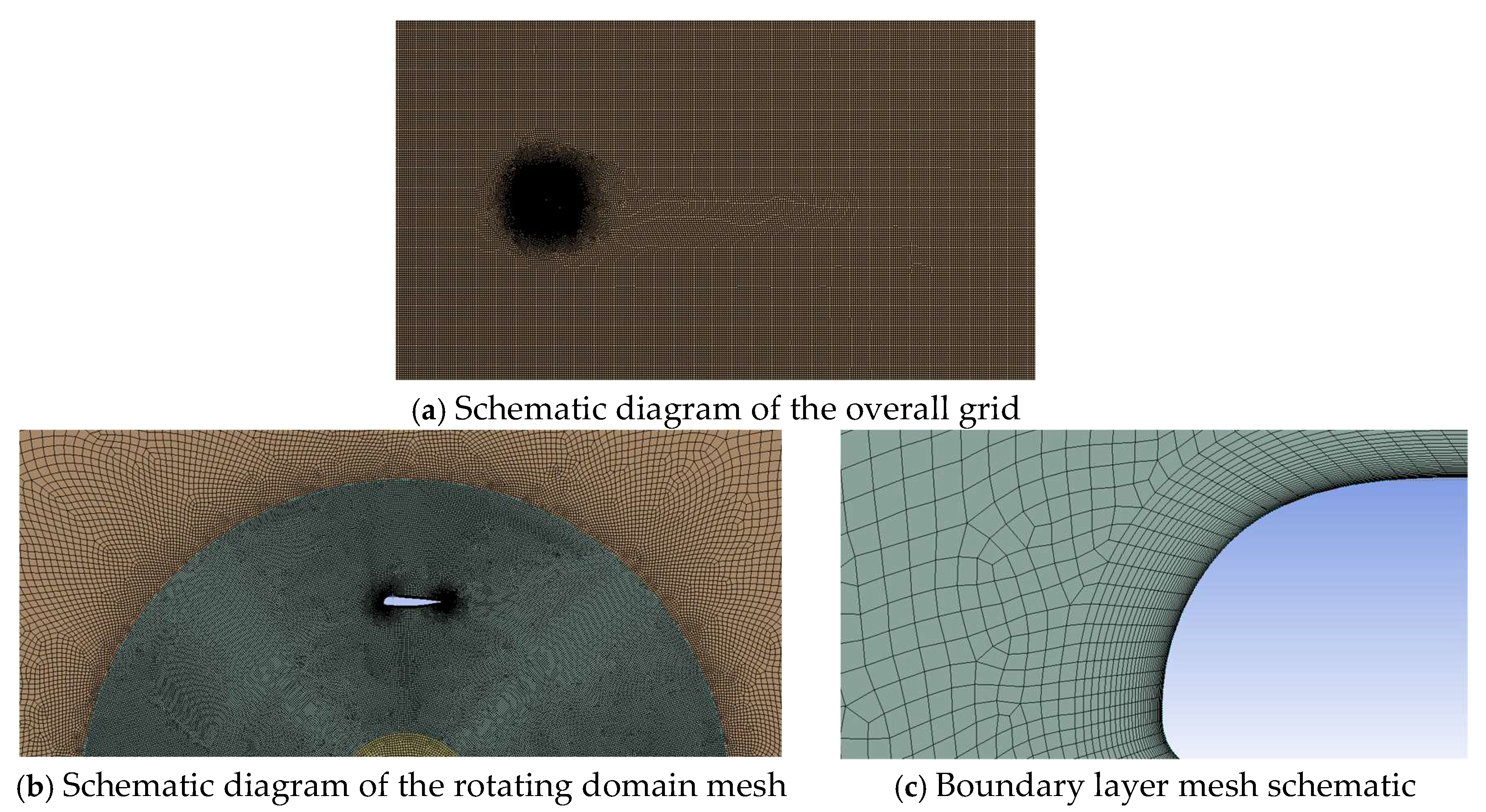
Meshing is a key step in CFD simulation, meshing is to discretize the continuous flow field into microelements for solving, which is of great significance and importance for the precision and accuracy of the simulation results. This paper involves a large amount of computational work and ANSYS Meshing software is selected to generate the mesh. As shown in Figure 11, a hybrid grid is used to discretize the computational domain, controlling the Y+ value to be less than 1, setting the height of the first layer of the grid to be 0.1 mm, and 1.1 as the growth rate of the boundary layer, and dividing a total of 30 layers.
Figure 11.
VAWT 2D mesh delineation knot result diagram.
4. Numerical Simulation Results
4.1. Model Validation
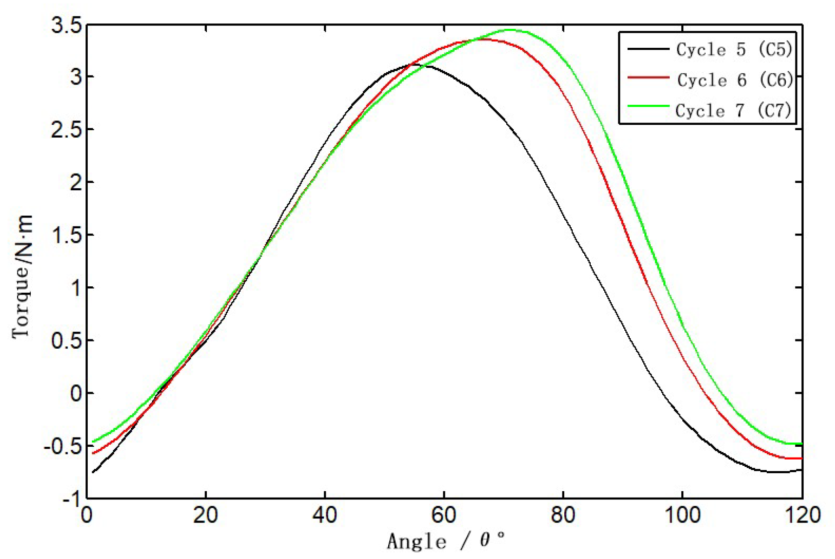
During numerical calculations, the wind turbine blades undergo a start-up transient phase within the first 3–5 rotational cycles, where the flow field has not yet developed stable periodic characteristics. This study employs a dynamic convergence criterion to evaluate transient results: the root-mean-square error (RMSE) of the average moment coefficient of the three blades over a single cycle is used as the convergence indicator. It is generally accepted in engineering practice that steady state is achieved when the RMSE between two consecutive cycles is less than 5%. Figure 11 presents the moment coefficient curves for the fifth to seventh cycles, with average values of 1.3932, 1.3596, and 1.3266, respectively. A relative error analysis reveals a 2.4% reduction from the sixth to seventh cycle, satisfying the engineering convergence standard. Consequently, the aerodynamic data from the seventh cycle are selected as the steady-state calculation results to ensure the accuracy of subsequent optimization analyses.
Figure 11.
Fifth, sixth and seventh cycle result curves.
A. Grid-independent verification
In this paper, three sets of grids are established for the model, the number of grids is 139310, 200320 and 385627, and the grid schematic is shown in Figure 12, respectively.
The moment coefficient versus azimuth change curves for the seventh cycle of the three different grid number models are shown in Figure 13, respectively, from which the results of the latter two sets of grid calculations basically overlap, and the gap with the first set of grids is larger. The average values of the moment coefficients of individual blades are 1.2129, 1.3266 and 1.3308, respectively, which shows that the difference of the second set of grids compared with the third set of moment coefficients is only 0.32%, and the second set of grids can satisfy the computational requirements by considering the comprehensive computational efficiency and computational accuracy.
B. Verification of time-step irrelevance
In this paper, the rotating domain is simulated in a transient manner using a slip grid, and the time step also has an important influence on the accuracy of the calculation results. In this paper, for the fan tip speed ratio of 1.5 conditions, a total of three-time steps is set, and the parameters corresponding to each time step are shown in Table 2.
The change curve of moment coefficient with the number of iterations in the seventh cycle of each time step is shown in Figure 14, respectively. Because the number of iterations is different, the running time of the seventh cycle is chosen as the horizontal coordinate, and it can be seen from the figure that the curve of the calculated results of each time-step blade rotated by 1° and each time-step blade rotated by 0.5° is basically overlapped with that of the calculated results, and the gap is larger with that of each time-step blade rotated by 2°, but each time-step blade rotated by 0.5° increases twice the calculation time. time-step blade rotation 0.5 ° doubles the calculation time, so the final synthesis of computational efficiency and calculation accuracy considerations, choose each time-step blade rotation 1 ° as the time step used in this paper's calculations.
C. Comparative validation of calculation results
For the wind turbine tip speed ratio of 0~2, this paper adopts the established calculation model to take 5 tip speed ratio for wind turbine power coefficient calculation and get its comparison curve with the test data as shown in Figure 15. The figure shows that the numerical calculation value is higher than the test value, and when the tip speed ratio is small, the two are closer, with the increase of the tip speed ratio, the error is getting bigger and bigger. The reason for this is that the 2D simulation assumes that the blade is of infinite length, which results in no flow along the spreading direction, while the actual wind turbine blade is of finite height, and the airflow will bypass the wingtip and flow from the surface of higher relative pressure to the surface of lower relative pressure, resulting in a pressure loss, so the test results are smaller than the simulation results is reasonable.
In response to the problem that the numerically calculated values are higher than the experimental values, Musgrove P proposed two correction factors for the turbine: one is the wind speed correction factor k and the other is the height correction factor τ, whose values are taken as 1.1 and 1.15, respectively, and the corrected tip-speed ratios and wind energy utilization of the turbine are:
The comparison curves of the modified power coefficient simulation values with the test values are shown in Figure 16. From the figure, the modified two-dimensional simulation results are basically the same as the trend of change with the test values, especially the simulation values at high tip speed ratio have very little error with the test values. This further proves the accuracy of the numerical calculation method adopted in this paper.
In this paper, the H-VAWT works in the high tip speed ratio working condition, comprehensive simulation analysis results and the use of installation requirements, selected the number of blades for 3, blade chord length of 0.42m, impeller rotational radius of 1.4m, this configuration as the optimization of the agent model of the basic configuration for research.
4.2. MIGA-Based H-VAWT Airfoil Optimization
Multi-Island Genetic Algorithm (MIGA) deals with complex optimization problems by dividing the population into multiple independently evolving islands, each of which independently performs the selection, crossover and mutation operations of traditional genetic algorithms (GA). Each island independently performs the selection, crossover and mutation operations of traditional GA. Individuals migrate between islands with a certain probability, to maintain the diversity of the population and effectively avoid the phenomenon of premature convergence, thus improving the ability of global optimization. Aiming at the problem of high computational cost of CFD evaluation in wind turbine airfoil optimization, an agent model is introduced to replace CFD simulation to reduce the computational cost and improve the optimization efficiency.
The optimization process begins with the construction of CFD sample data for the wind turbine, establishing a CFD database based on the initial airfoil to provide training data. Subsequently, an initial population P0 is randomly generated, and the evolution generation count is set to n =0. During the evolutionary process, the multi-island parallel evolution mechanism enables independent GA optimization within each island. After each generation, the system determines whether to perform migration operations: if migration conditions are met, individual exchanges occur between islands to enhance global search capabilities; otherwise, independent evolution continues. This process iterates until the maximum generation limit or convergence criteria.
In the optimization process, the agent model plays a central supporting role in the evolution of the MIGA. When the genetic algorithm generates a new population, the proxy model can quickly predict the aerodynamic performance of the airfoil, thus reducing the frequency of direct calls to the CFD simulation and significantly reducing the computational cost. After the optimization is completed, the optimal individuals need to be verified by CFD to check the prediction accuracy of the proxy model. Based on the validated optimization results, the key parameters of the airfoil are further adjusted, and the optimal airfoil configuration is finally determined through comprehensive evaluation to complete the airfoil optimization design. The coefficient of determination R2 measures the accuracy of the kriging substitution model and can be expressed as:
In the formula, is the number of test sample points, is the experimental value, is the estimate of the proxy model, and is the mean of the experimental point set.
The co-optimization flow of MIGA and the proxy model is shown in Figure 17, which demonstrates the significant advantages of the method in the airfoil optimization. MIGA significantly enhances the global search capability through the parallel evolution and migration strategy, while the introduction of the proxy model significantly reduces the frequency of CFD simulation calls. This efficient coupling method can achieve high-quality airfoil optimization under limited computational resources and provides a reliable optimization strategy for wind turbine aerodynamic design.
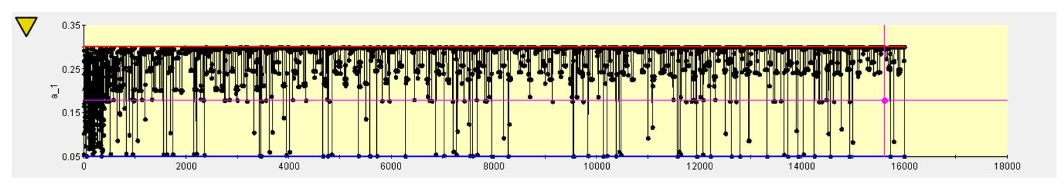
The H-VAWT airfoil in this paper contains a total of 12 parameters of the CST method and one parameter of the mounting angle, and from the previous analysis, it is known that the greater impact on the aerodynamic performance of the wind turbine is the leading edge radius, the airfoil thickness, the trailing edge shape and the mounting angle, and each parameter of the CST method has a specific meaning, so in this paper, we choose a total of seven parameters, namely, a1, a2, a6, b1, b2, b6 and the mounting angle α as the optimization variables, the sample points for agent model construction are determined as ten times the number of parameters, i.e., 70 sample points, and the error analysis points are taken as 10.
The sensitivity analysis of the influence of each parameter on the power extraction coefficient of the wind turbine is shown in Figure 18 and Figure 19, which shows that the power extraction coefficient is the most sensitive to the radius of the leading edge, followed by the relative thickness, and finally the shape of the trailing edge, so that the reasonable design of the radius of the leading edge is the most critical to the power extraction coefficient of the wind turbine. Figure 18 shows the results of the error analysis of the constructed proxy model, and the L2 value of the error analysis is 0.91368, which is generally accepted in engineering greater than 0.8, and the results show that the fitting accuracy is high, and it can be used to optimize the design.
Taking 10 populations with 40 samples for each population and a total of 40 iterations, the final parameters of the two optimized configurations are shown in Table 3, respectively. As shown in Figure 20 and Figure 21, the optimization was calculated for a total of 16,000 times, and basically reached convergence around the 4,000th time, compared with the original configuration, the power extraction coefficients of the optimized configuration 1 were improved by 14.2%, and the power extraction coefficients of the optimized configuration 2 were improved by 11.6%, and the two configurations both played a better optimization effect.
Figure 20.
Iterative diagram of the optimization process for optimized configuration 1.
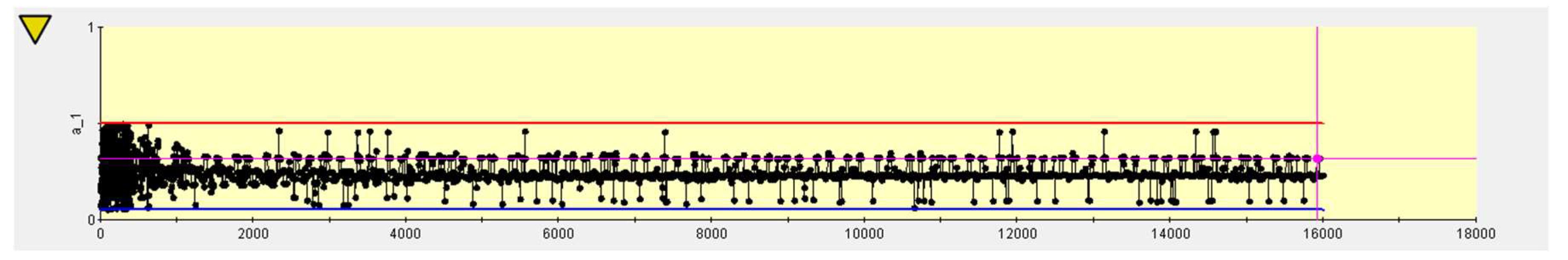
Figure 21.
Iterative diagram of the optimization process for optimized configuration 2.
Comparison of optimized front and rear airfoil shapes is shown in Figure 22. Compared to the original symmetric airfoil, both optimized airfoils have positive mounting angles, and the upper airfoil is fuller than the lower airfoil, and the thickness of the trailing edge is relatively larger, and the relative thickness and mounting angle of the optimized configuration 2 are smaller than those of the optimized configuration 1.
Figure 23 demonstrates the variation pattern of the wind turbine power coefficient with tip speed ratio calculated using McLaren's correction formula before and after optimization. From the figure, it can be seen that the power coefficients of both optimized airfoils are significantly better than the original airfoils in the whole range of tip speed ratios. Under the low tip speed ratio condition, the power coefficient enhancement of optimized airfoil type 1 and optimized airfoil type 2 are basically equal, but the maximum power extraction coefficient of optimized airfoil type 1 is larger than that of airfoil type 2. The results show that the two optimized airfoils have similar starting performance under low tip speed ratio conditions, but from the aerodynamic aspect of high tip speed ratio, the optimized airfoil 1 is optimized for airfoil 2.
Figure 24 demonstrates the variation rule of moment coefficient with azimuth angle for individual blades before and after optimization when the tip speed ratio is 1.8, and the horizontal coordinate indicates the azimuth angle of blade rotation. The results show that the main power output of the blades is concentrated in the 50°~180° azimuth interval, and the power generated by the remaining azimuth region is smaller. Due to the cyclic rotational characteristics of the three-bladed wind turbine, each blade will enter the 50°~180° azimuth region alternately, so as to maintain the continuous operation of the wind turbine effectively. After optimization, the wind turbine not only improves the maximum moment coefficient of the blades, but also improves the moment coefficient of the blades in most of the azimuthal angles, so that the power coefficient of the wind turbine as a whole is improved.
4.3. Optimization Results Analysis
A. Comparative analysis of pressure distribution
Figure 25 shows comparatively the pressure distribution clouds of the original configuration, optimized configuration 1 and optimized configuration 2 at different azimuthal angles when the tip speed ratio is 1.8, and the legends are the same in all the figures for the sake of comparison. The comparative analysis shows that the optimized H-VAWT exhibits significant aerodynamic performance enhancement at different azimuth angles. Specifically, in the range of 60°-120° key azimuth angle, the optimized blade surface pressure gradient distribution is more uniform, the leading edge high-pressure zone area is reduced, and the trailing edge low-pressure zone pressure value is increased, which effectively reduces the pressure drag loss, and overall improves the wind energy utilization of the wind turbine. At the same time, the results of the flow field diagram show that the optimized design effectively reduces the flow separation and turbulence area, the flow line is smoother, and the flow adhesion on the surface of the wind turbine blade is improved, which reduces the drag and improves the performance. These optimization results show that the improved airfoil design has significant advantages in pressure distribution and aerodynamic efficiency, which enhances the overall performance and energy capture capability of the wind turbine. The main effect of the optimization is to improve the lift effect of the airfoil in an integrated way, since the airfoil angle of approach is not changed, so the direction of the lift force remains unchanged, which in turn can provide a larger torque.
B. Comparative analysis of speed distribution
Figure 26 represents the comparison of the velocity distribution cloud plots of the original configuration, optimized configuration 1 and optimized configuration 2 at different azimuthal angles when the modified tip speed ratio is 1.8, respectively, and the legends of all the plots are the same in order to facilitate the comparison, from which it can be seen that all the three configurations are rotating for one week. According to the velocity cloud plots at different azimuthal angles, the optimized H-VAWT shows significant improvement in fluid characteristics.
The optimized design results in a more uniform flow over the blade surface, especially at the 0° and 60° positions, where the flow structure is smoother, reducing vortices and flow separation phenomena, thus reducing energy losses. At the 120° position, the optimized design significantly improves the adhesion of the flow lines, reduces unnecessary energy consumption, and enhances the aerodynamic efficiency. Further analysis of the flow distribution at azimuth angles of 180° and 240° shows that the optimized model exhibits smoother flow at the trailing edge of the blade and near-tail region, improving the wind energy conversion capability. The explanation for the more pronounced vortex shedding phenomenon of the original configuration after azimuth angle 240° may be related to the changes in the design parameters of the airfoil. Specifically, the primitive configuration at this azimuth angle may lead to accelerated changes in the airflow or increased local pressure differences, which exacerbate airflow separation and lead to more pronounced vortex shedding in the wake.
Finally, at 300°, the optimized design similarly improves the flow uniformity, reduces vortex formation, and enhances the wind energy capture capability of the blade. Overall, the optimized design reduces the flow resistance and energy loss by improving the fluid characteristics of the wind turbine, thus effectively enhancing the overall performance and efficiency of the wind turbine. With an azimuth angle greater than 90°, the airfoil appears to stall and a trailing vortex is generated at the trailing edge, which increases drag and reduces aerodynamic performance. The optimized airfoil is able to provide greater torque by improving the flow field characteristics, weakening the airflow separation, reducing drag, and reducing the negative torque generated by the drag, which also demonstrates the effectiveness of the optimized design in reducing drag and increasing torque.
5. Conclusions
This paper systematically analyzes the effects of the number of wind turbine blades, blade chord length and rotation radius on wind energy utilization, and describes the mechanism of these key design parameters on aerodynamic performance under different tip-speed ratio operating conditions. Based on the optimization analysis, a wind turbine with blade number of 3, blade chord length of 0.42 m and rotation radius of 1.4 m is selected as the best design basis.
Meanwhile, a hybrid optimization strategy of Kriging agent model combined with MIGA is proposed in this paper to optimize the airfoil configuration of H-VAWT. The optimization results show that the optimized airfoil significantly improves the power extraction capability of the wind turbine. Among them, the optimized configuration 1 shows better aerodynamic performance under high tip-speed ratio conditions, and its maximum power extraction coefficient is increased by 14.2% compared with the original configuration. During the optimization process, through the fine adjustment of key parameters such as airfoil thickness and mounting angle, the optimized wind turbine not only improves the moment coefficient of the blade, but also significantly enhances the power output capability especially in the range of 50°~180° azimuthal angle, which further improves the overall power extraction efficiency of the wind turbine. The optimization method proposed in this study not only provides a systematic theoretical basis for the design of wind turbine airfoils, but also provides an effective technical support for improving the aerodynamic performance and energy conversion efficiency of wind turbines.
References
- Badiei, D.; Sadr, H.M.; Shams, S. Nonlinear aeroelasticity of H-type vertical axis wind turbine blade. Journal of Wind Engineering & Industrial Aerodynamics 2024, 246105656.
- Hao, W.; Li, C.; Wu, F. Adaptive blade pitch control method based on an aerodynamic blade oscillator model for vertical axis wind turbines. Renewable Energy 2024, 223120114. [Google Scholar] [CrossRef]
- Zhao, B.; Ma, H.P.; Zhao, Y.X.; et al. Application analysis of vertical axis wind turbine in plateau areas. Journal of Drainage and Irrigation Machinery Engineering 2018, 36, 7. [Google Scholar]
- Jiang, Y.; Chen, P.; Wang, S.; et al. Dynamic responses of a 5 MW semi-submersible floating vertical-axis wind turbine: A model test study in the wave basin. Ocean Engineering 2024, 296117000. [Google Scholar] [CrossRef]
- Jemal, T.; Shimels, S.; Ali, Y.; et al. Impact of Turbulent Flow on H-Type Vertical Axis Wind Turbine Efficiency: An Experimental and Numerical Study. International Journal of Heat and Technology 2023, 41. [Google Scholar] [CrossRef]
- A, Xinyu Zhu; et al. Numerical study of aerodynamic characteristics on a straight-bladed vertical axis wind turbine with bionic blades. (2021).
- Mohammed, Amin A; et al. Vertical Axis Wind Turbine Aerodynamics: Summary and Review of Momentum Models. Journal of Energy Resources Technology 2019, 141, 050801.1–05080110.
- Marini, M.; Massardo, A.; Satta, A. Performance of vertical axis wind turbines with different shapes. Journal of Wind Engineering & Industrial Aerodynamics 1992, 39, 83–93. [Google Scholar]
- Deshmukh, S.; Charthal, S. Design and Development of Vertical Axis Wind Turbine. 2017. [CrossRef]
- Haitian, Z.; Chun, L.; Wenxing, H.; et al. Investigation on aerodynamic characteristics of building augmented vertical axis wind turbine. Journal of Renewable and Sustainable Energy 2018, 10, 053302. [Google Scholar] [CrossRef]
- Shah, S.R.; Kumar, R.; Raahemifar, K.; et al. Design, modeling and economic performance of a vertical axis wind turbine. Energy Reports 2018, 4, 619–623. [Google Scholar] [CrossRef]
- Halawa, T. Numerical and Experimental Investigation of the Performance of a Vertical Axis Wind Turbine Based on the Magnetic Levitation Concept. Journal of Energy Resources Technology 2022. [CrossRef]
- Mohammed, A.A.; Sahin, A.Z.; Ouakad, H.M. Numerical Investigation of a Vertical Axis Wind Turbine Performance Characterization Using New Variable Pitch Control Scheme. Journal of Energy Resources Technology 2020, 142. [Google Scholar] [CrossRef]
- Reyes, V.; Carranza, O.; Rodríguez, J.; et al. Comparative Study of the Performance of Wind Turbines in relation to both Power and Torque Coefficients. Revista Politécnica 2018, 41, 7–16. [Google Scholar]
- Hand, B.; Kelly, G.; Cashman, A. Aerodynamic design and performance parameters of a lift-type vertical axis wind turbine: A comprehensive review. Renewable and Sustainable Energy Reviews 2021, 139. [Google Scholar] [CrossRef]
- Ma, N.; Lei, H.; et al. Airfoil optimization to improve power performance of a high-solidity vertical axis wind turbine at a moderate tip speed ratio. Energy 2018, 150, 236–252. [Google Scholar] [CrossRef]
- Lee, Y.-T.; Lin, H.-C. Numerical study of the aerodynamic performance of a 500 W Darrieus-type vertical-axis wind turbine. Renewable Energy 2015, 83, 407–415. [Google Scholar] [CrossRef]
- Ghasemian, M.; Ashrafi, Z.N.; Sedaghat, A. A review on computational fluid dyna mic simulation techniques for Darrieus vertical axis wind turbines. Energy Conversion and M anagement 2017, 149, 87–100. [Google Scholar] [CrossRef]
- Liang, C.; Li, H. Aerofoil optimization for improving the power performance of a vertical axis wind turbine using multiple streamtube model and genetic algorithm. Royal Society Open Science 2018, 5, 180540. [Google Scholar] [CrossRef] [PubMed]
- Peng, Y.; Xu, Y.; Zhan, S. A hybrid DMST model for pitch optimization and performance assessment of high-solidity straight-bladed vertical axis wind turbines. Applied Energy 2019, 250, 215–228. [Google Scholar] [CrossRef]
- Jayakrishnan, R.; Surya, S.; Mohammed, Z.; et al. Design optimization of a Contra-Rotating VAWT: A comprehensive study using Taguchi method and CFD. Energy Conversion and Management 2023, 298. [Google Scholar]
- Zhou,Donghai,Zhou; et al. Performance enhancement of straight-bladed vertical axis wind turbines via active flow control strategies: a review. Meccanica 2021, 57, 1–28.
- Tian, X.; Li, J. Robust aerodynamic shape optimization using a novel multi-objective evolutionary algorithm coupled with surrogate model. Structural and Multidisciplinary Optimization 2020, 62, 1969–1987. [Google Scholar] [CrossRef]
Figure 2.
Schematic diagram of wing structure parameters.
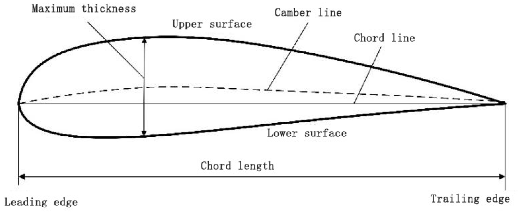
Figure 3.
Schematic diagram of aerodynamic forces on an airfoil.
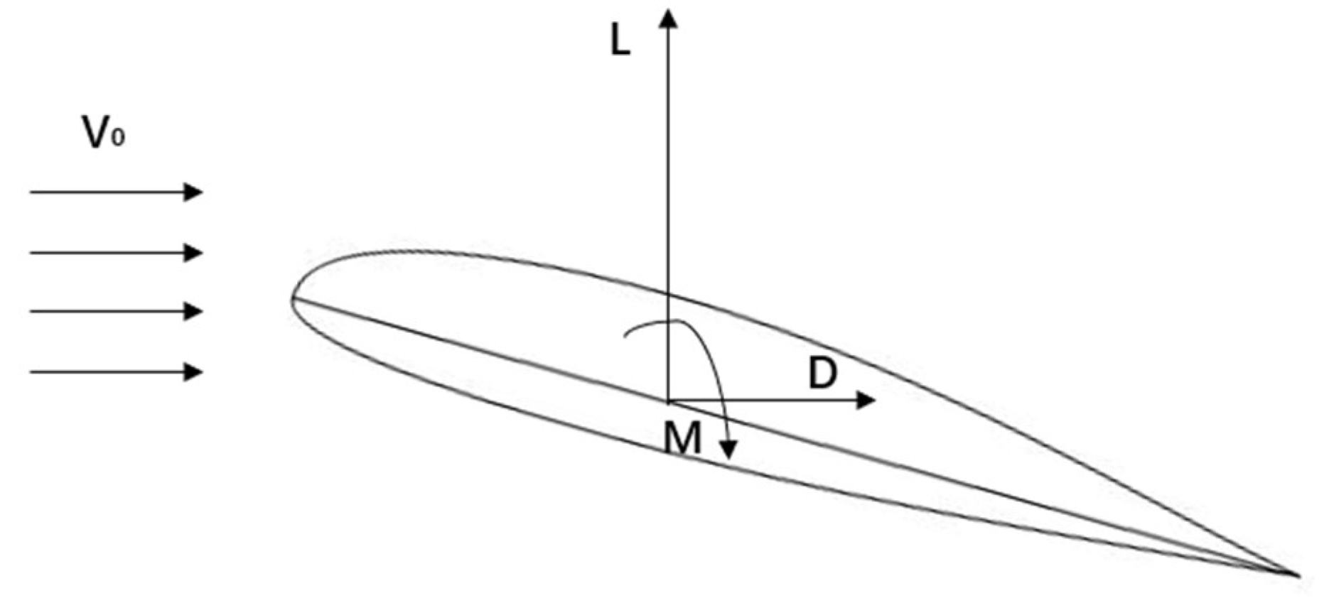
Figure 4.
Force diagram of airfoil.
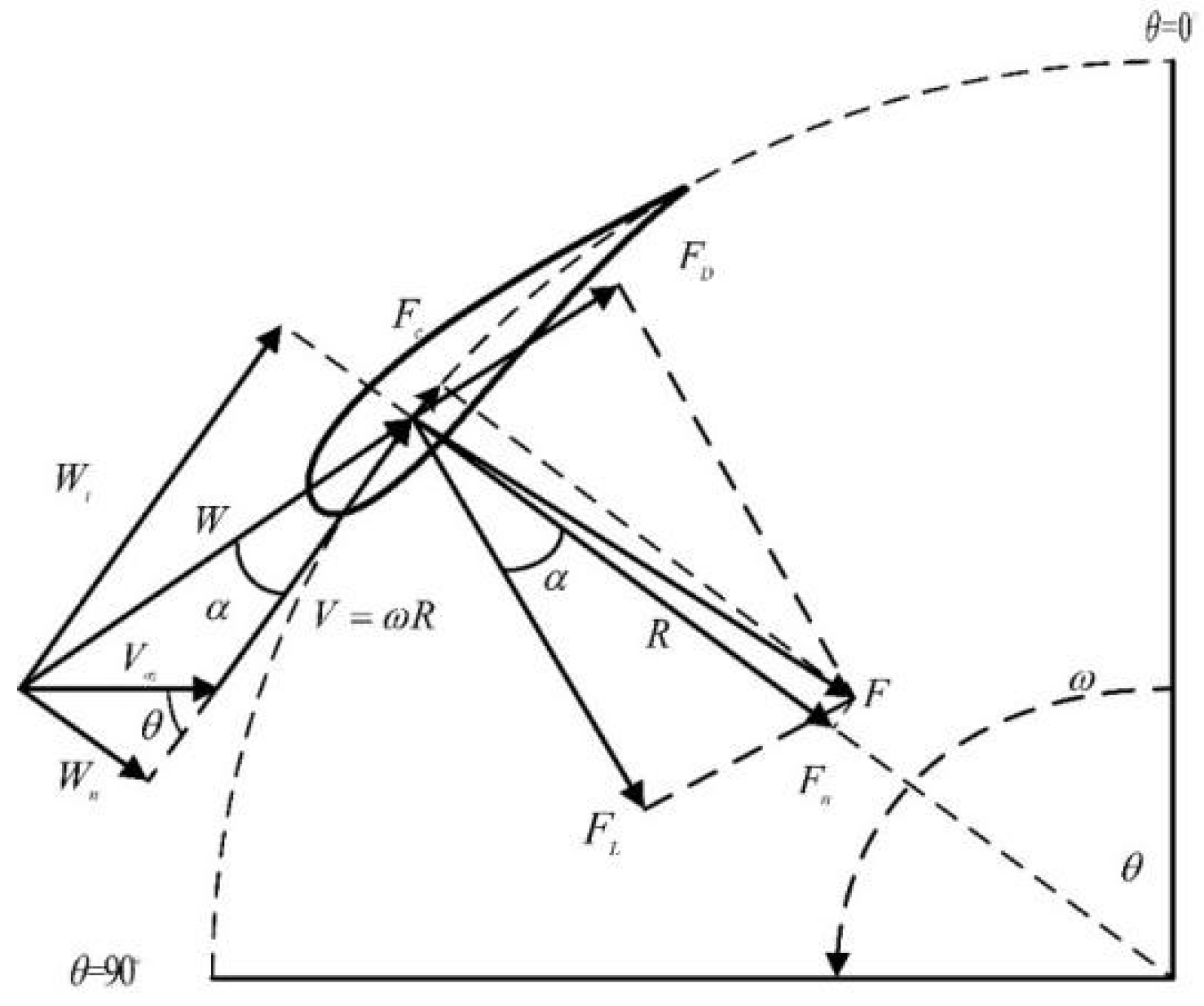
Figure 5.
Schematic of VAWT blade forces at different azimuthal angles.
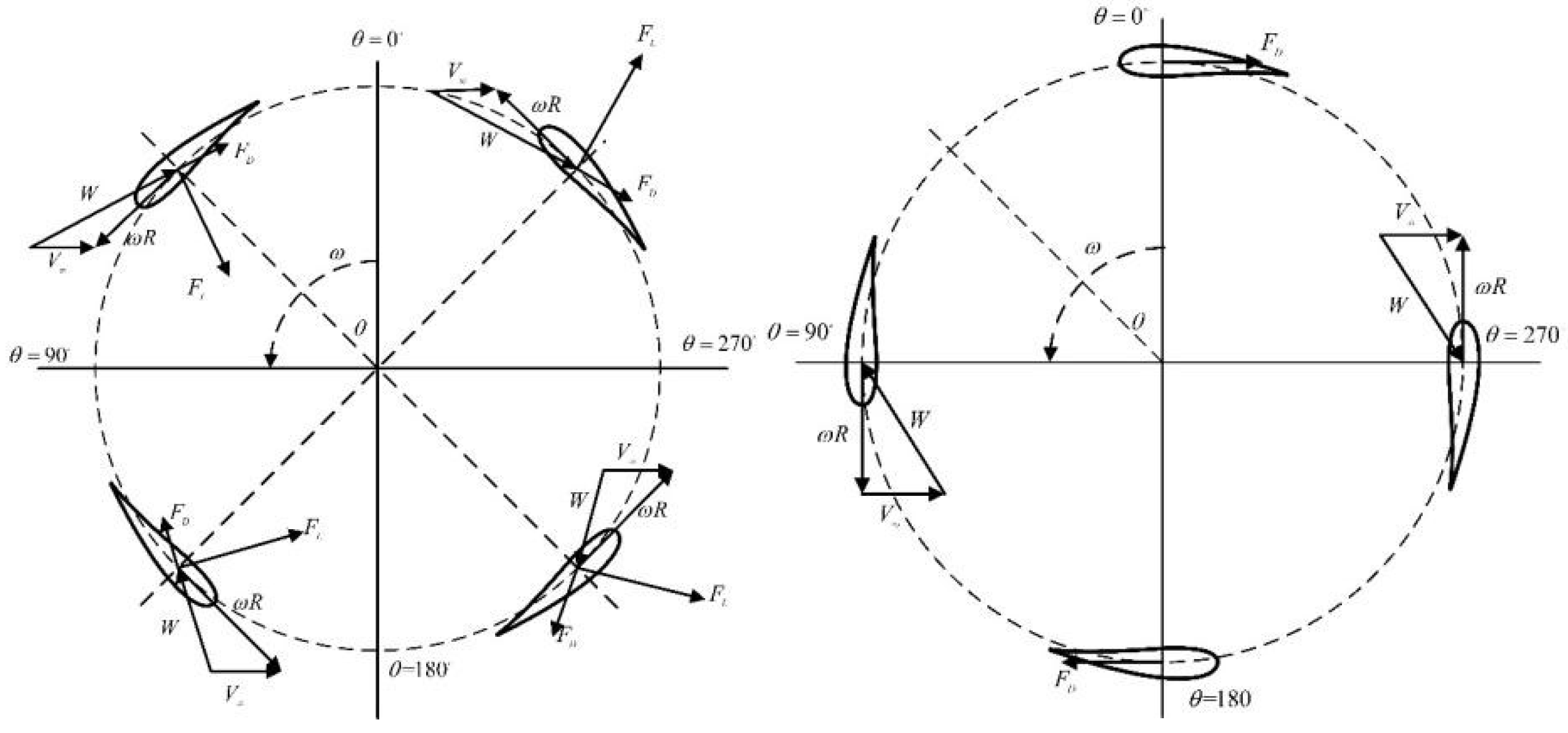
Figure 8.
NACA0015 wing CST fitting results.
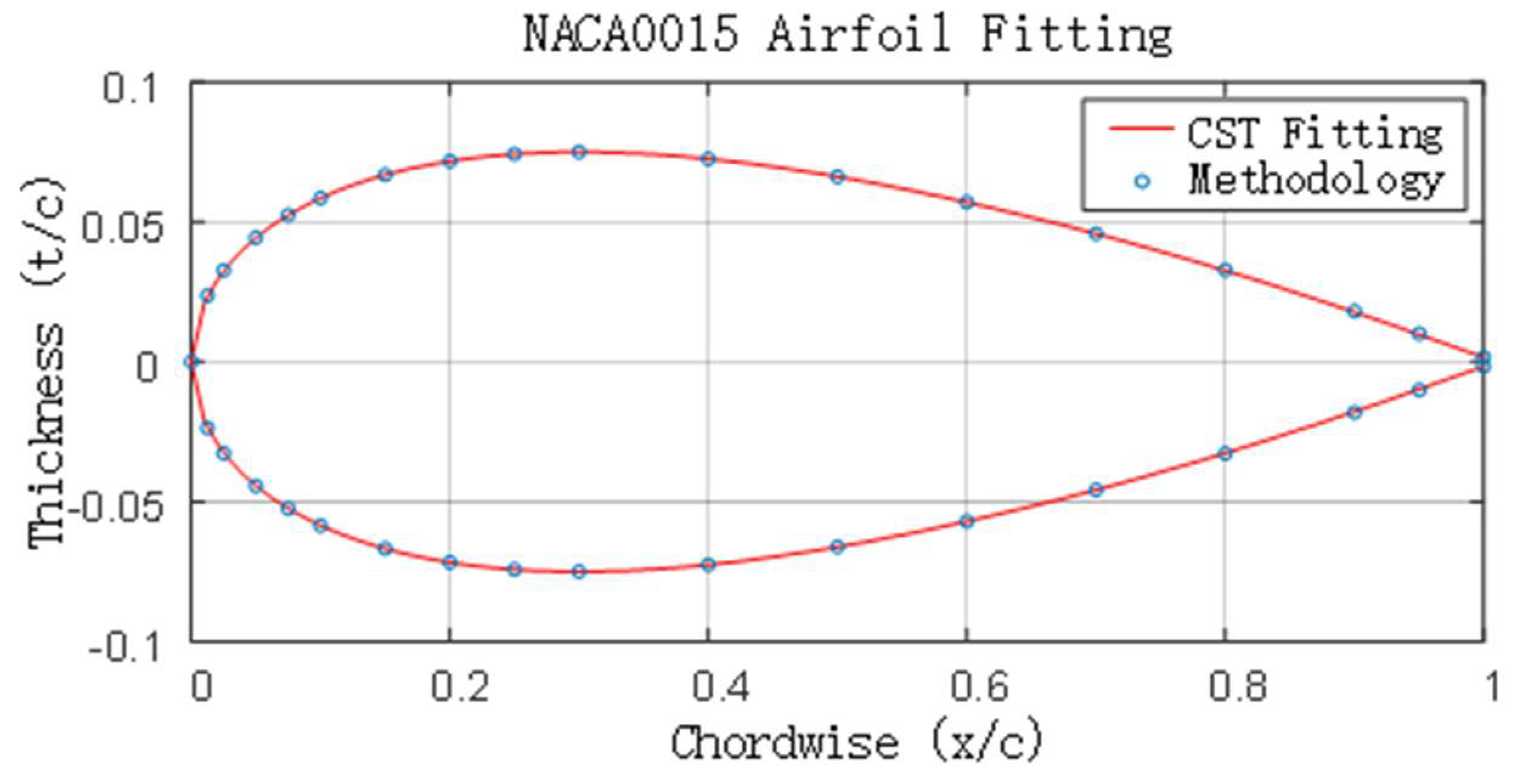
Figure 9.
Musgrove P test blade arrangement.
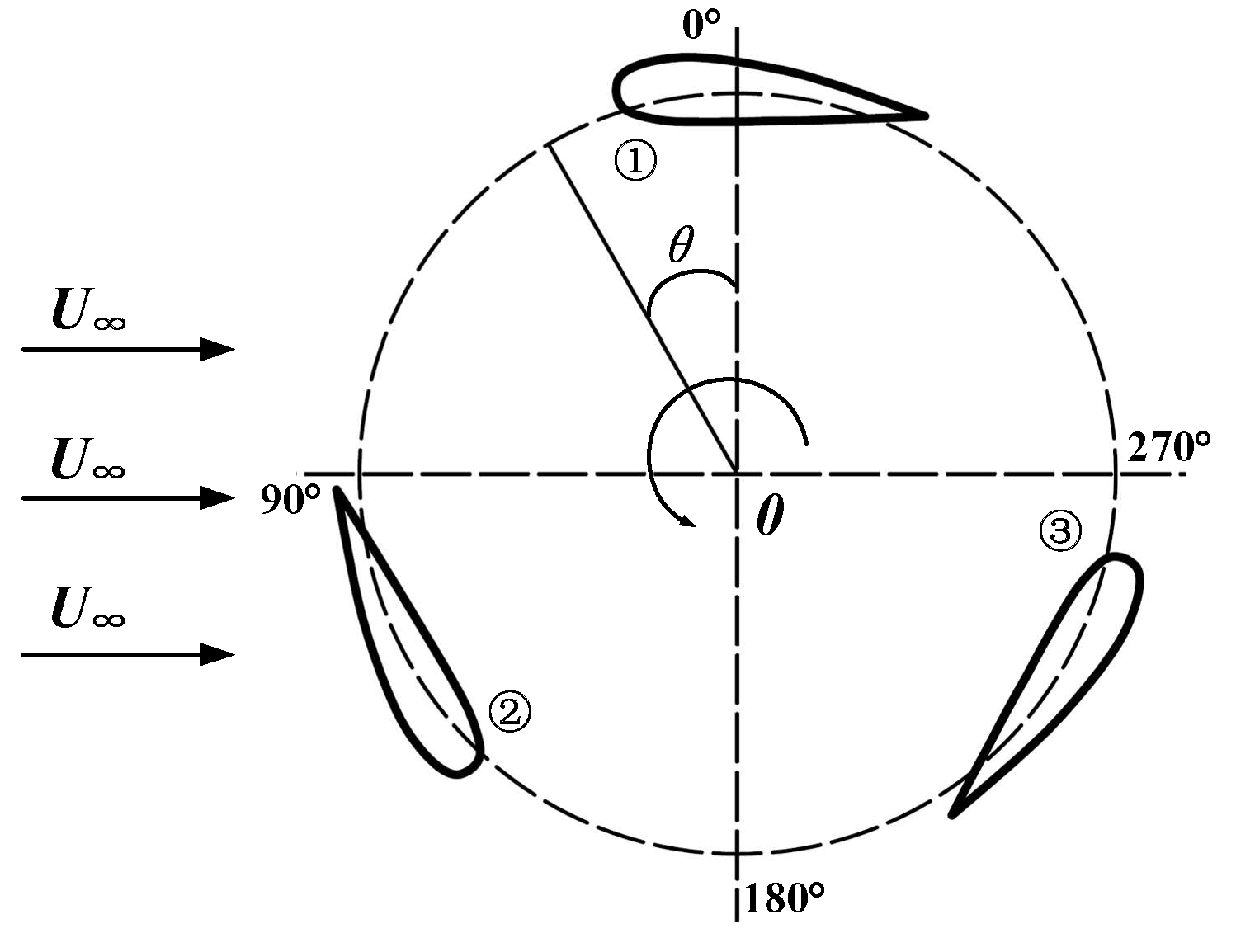
Figure 10.
VAWT schematic diagram of the flow field scale.

Figure 12.
Schematic diagram of a grid-independent verification grid.
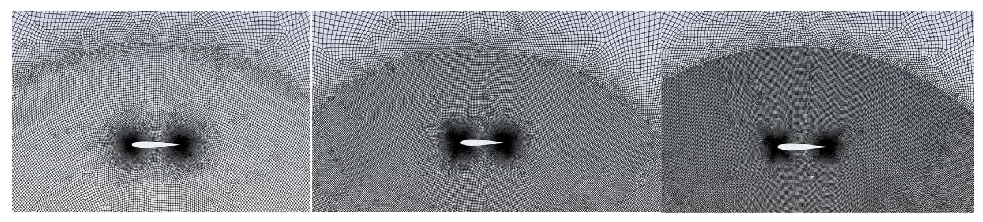
Figure 13.
Schematic comparison of moment coefficients for mesh-independence validation.
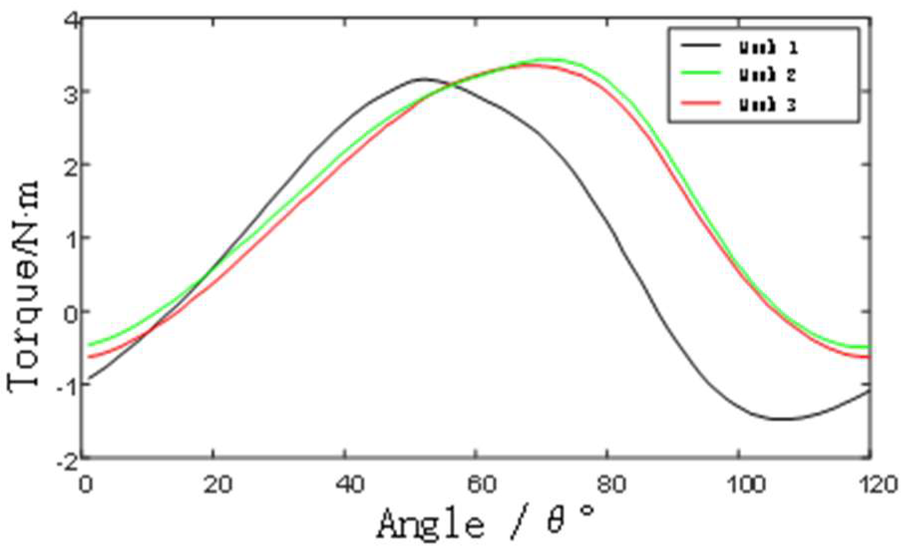
Figure 14.
Schematic comparison of moment coefficients for time-step independence validation.
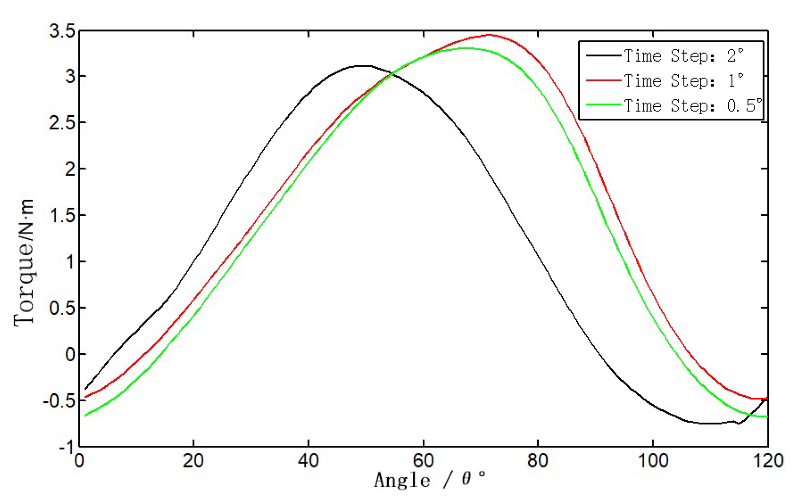
Figure 15.
Comparison of simulation results with tests.
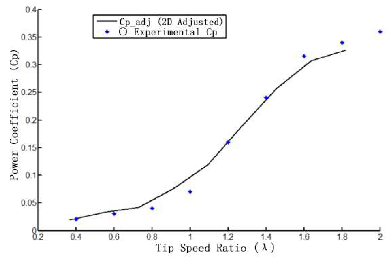
Figure 16.
Schematic diagram of comparison between simulated and experimental values after correction.
Figure 16.
Schematic diagram of comparison between simulated and experimental values after correction.
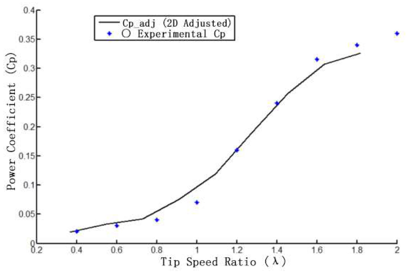
Figure 17.
MIGA and Agent Model Optimization Flowchart.
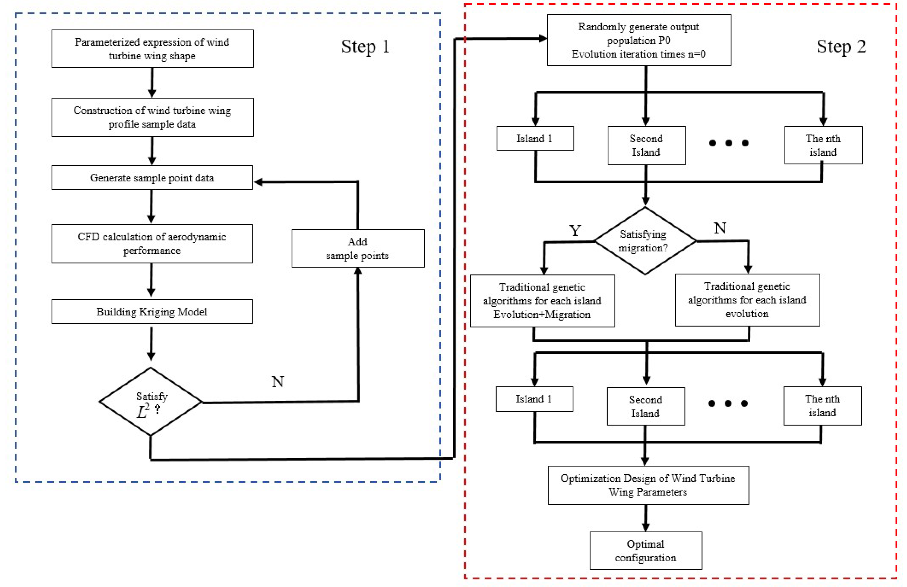
Figure 18.
Schematic of parameter sensitivity analysis.
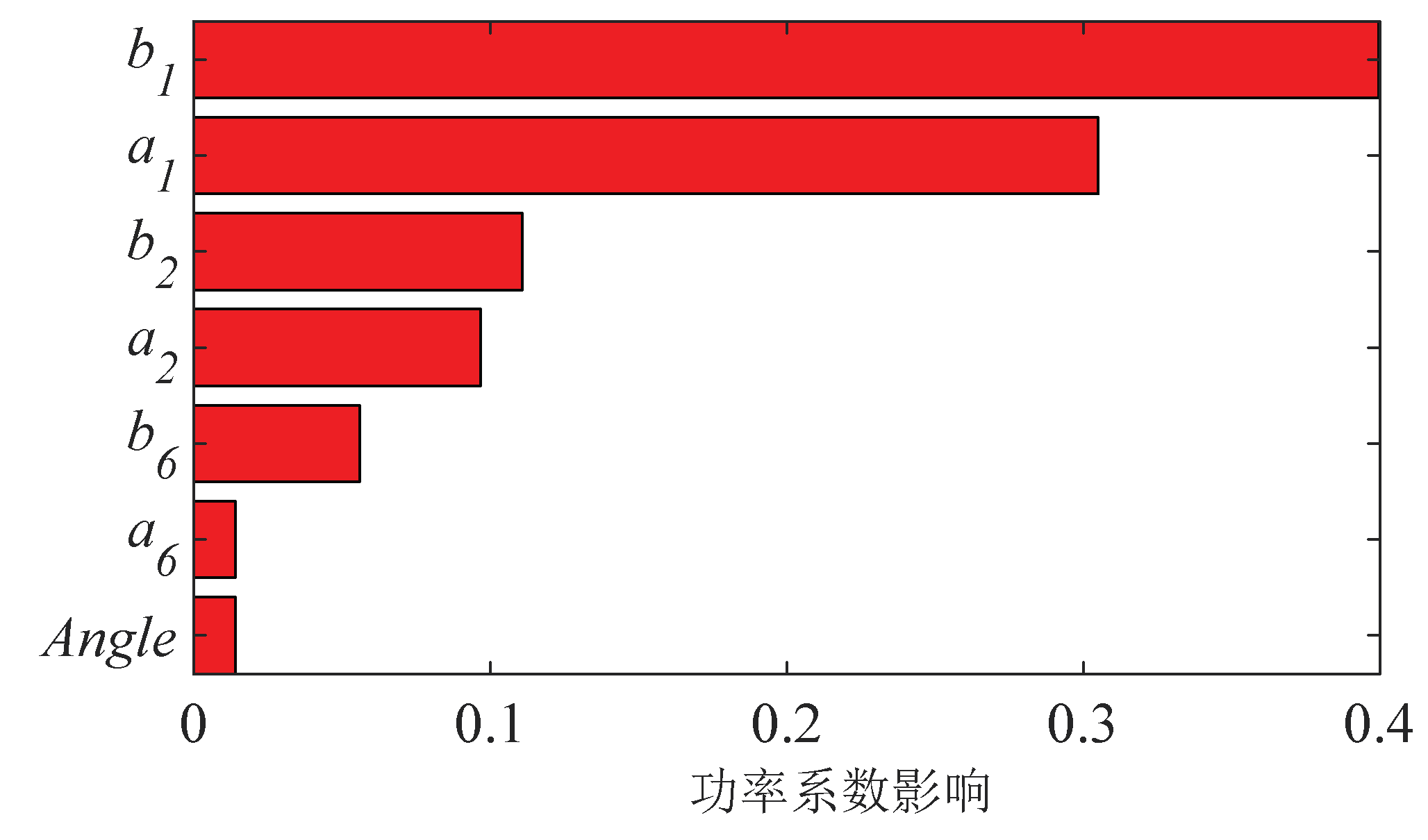
Figure 19.
Schematic diagram of the error analysis of the proxy model.
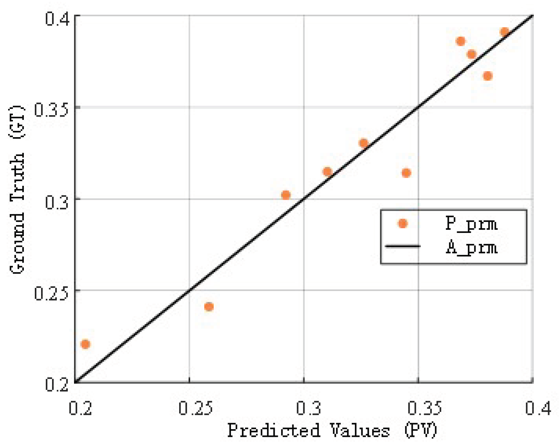
Figure 22.
Optimized configuration vs. original configuration.
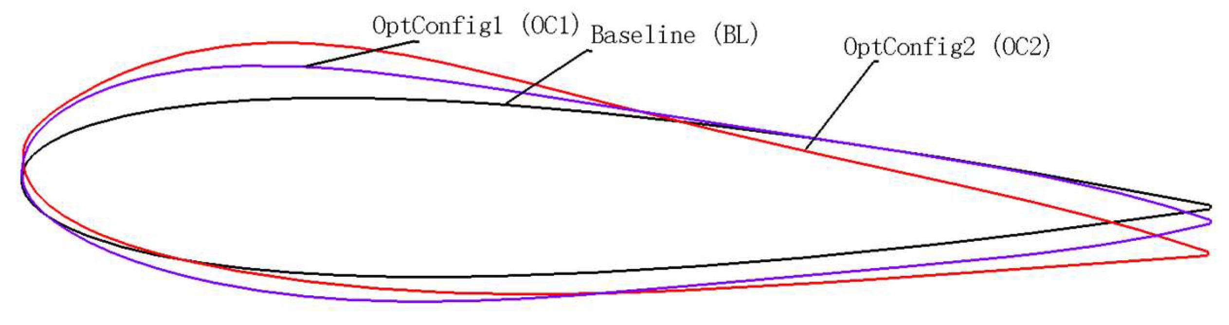
Figure 23.
Comparison of power extraction coefficient results between optimized and original configurations.
Figure 23.
Comparison of power extraction coefficient results between optimized and original configurations.
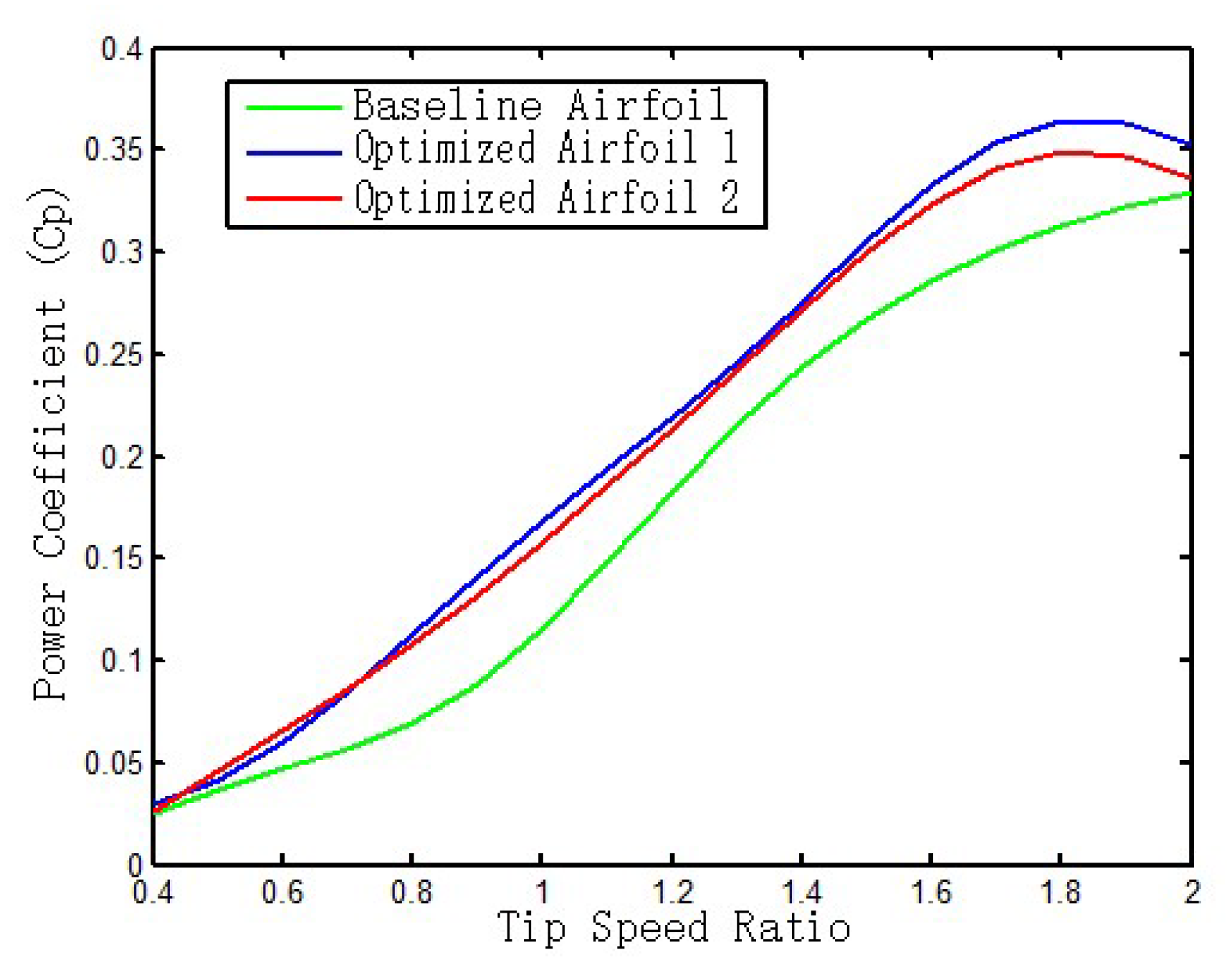
Figure 24.
Comparison of individual blade results between optimized and original configurations.
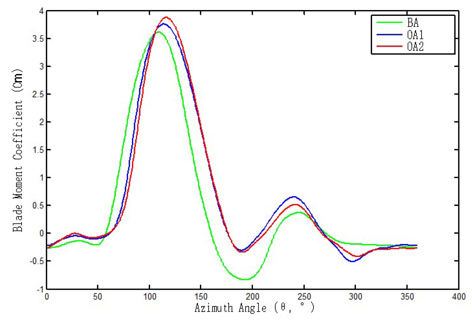
Figure 25.
Cloud map of pressure distribution at different azimuths.
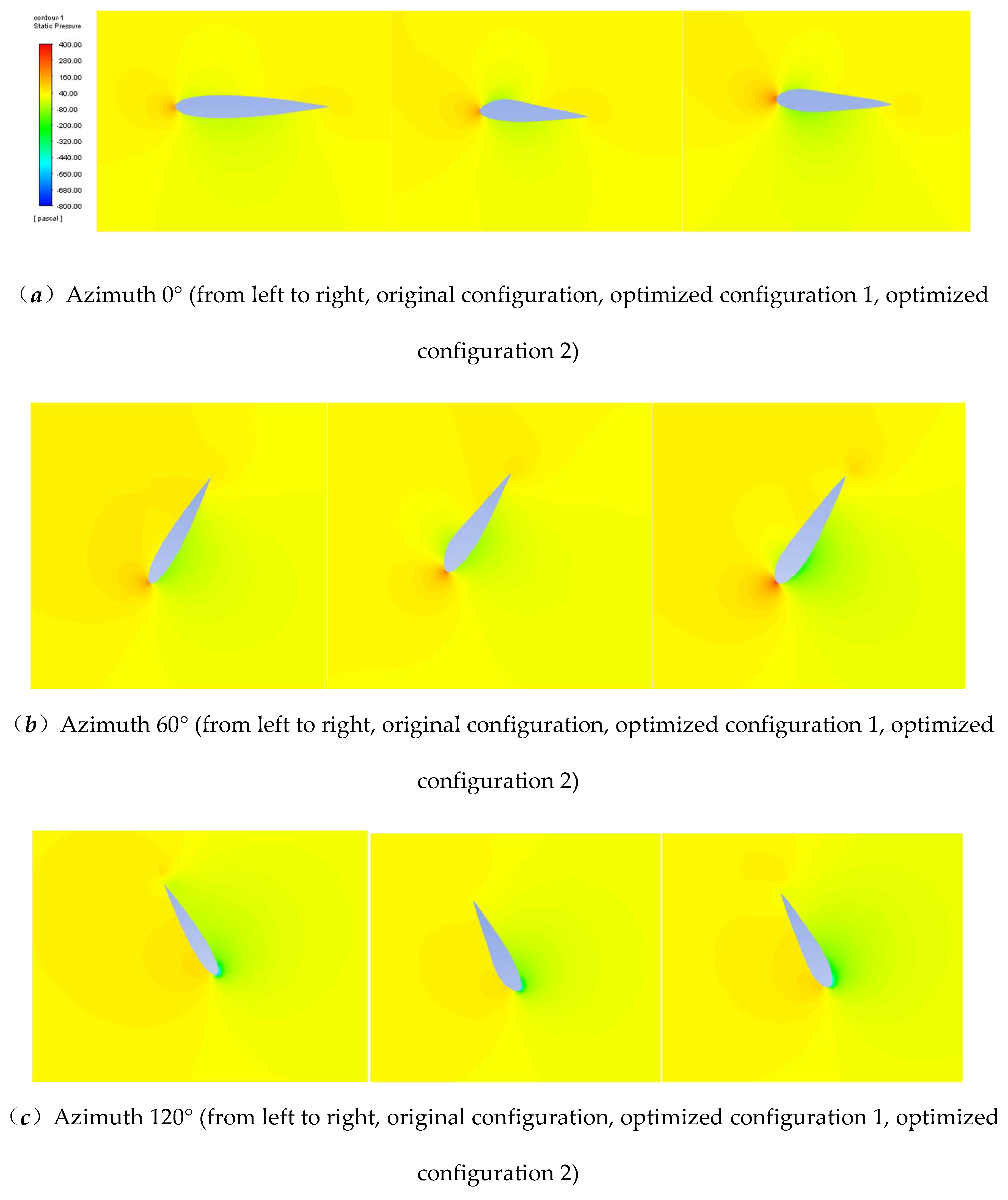
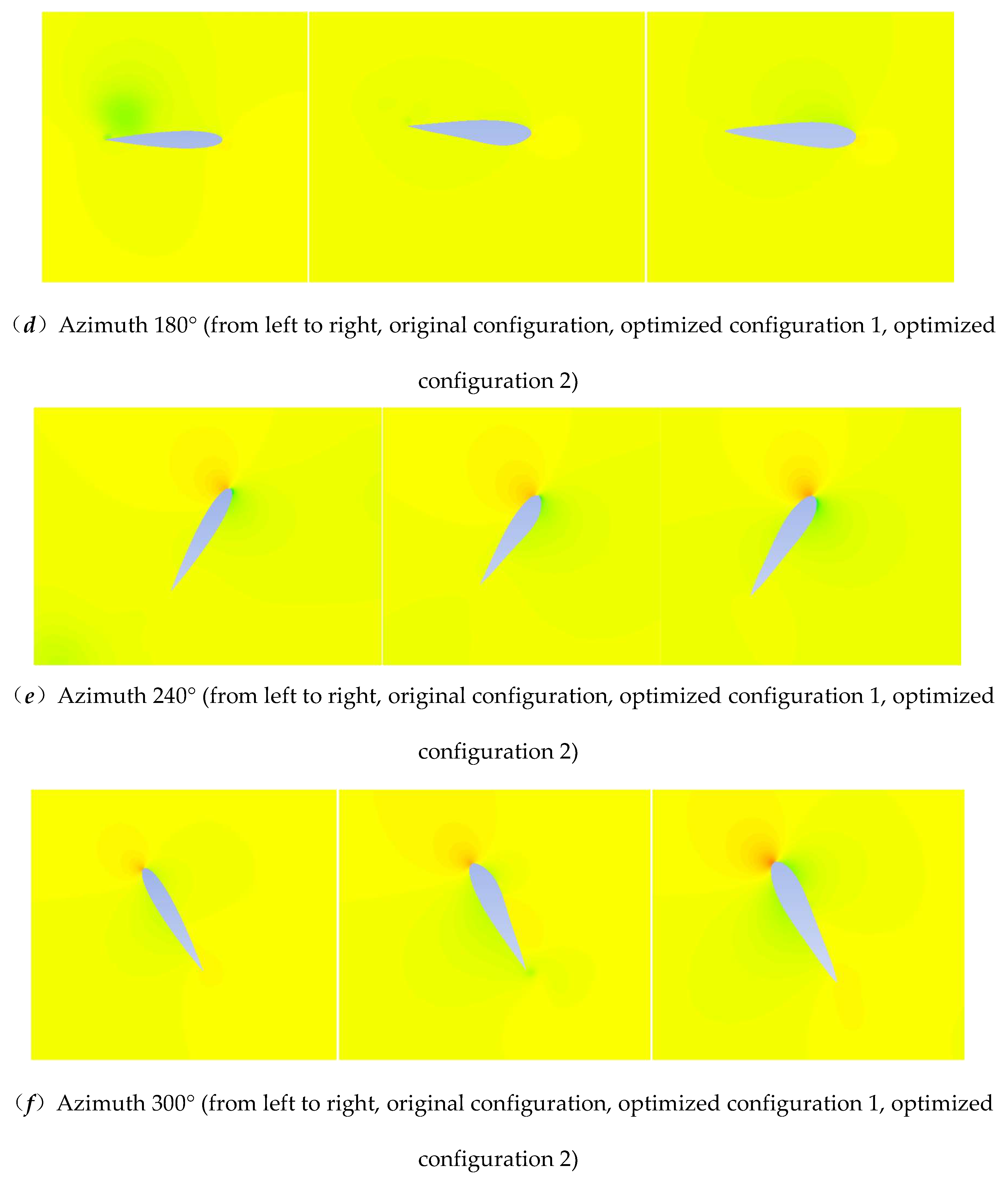
Figure 26.
Velocity clouds in different azimuths.
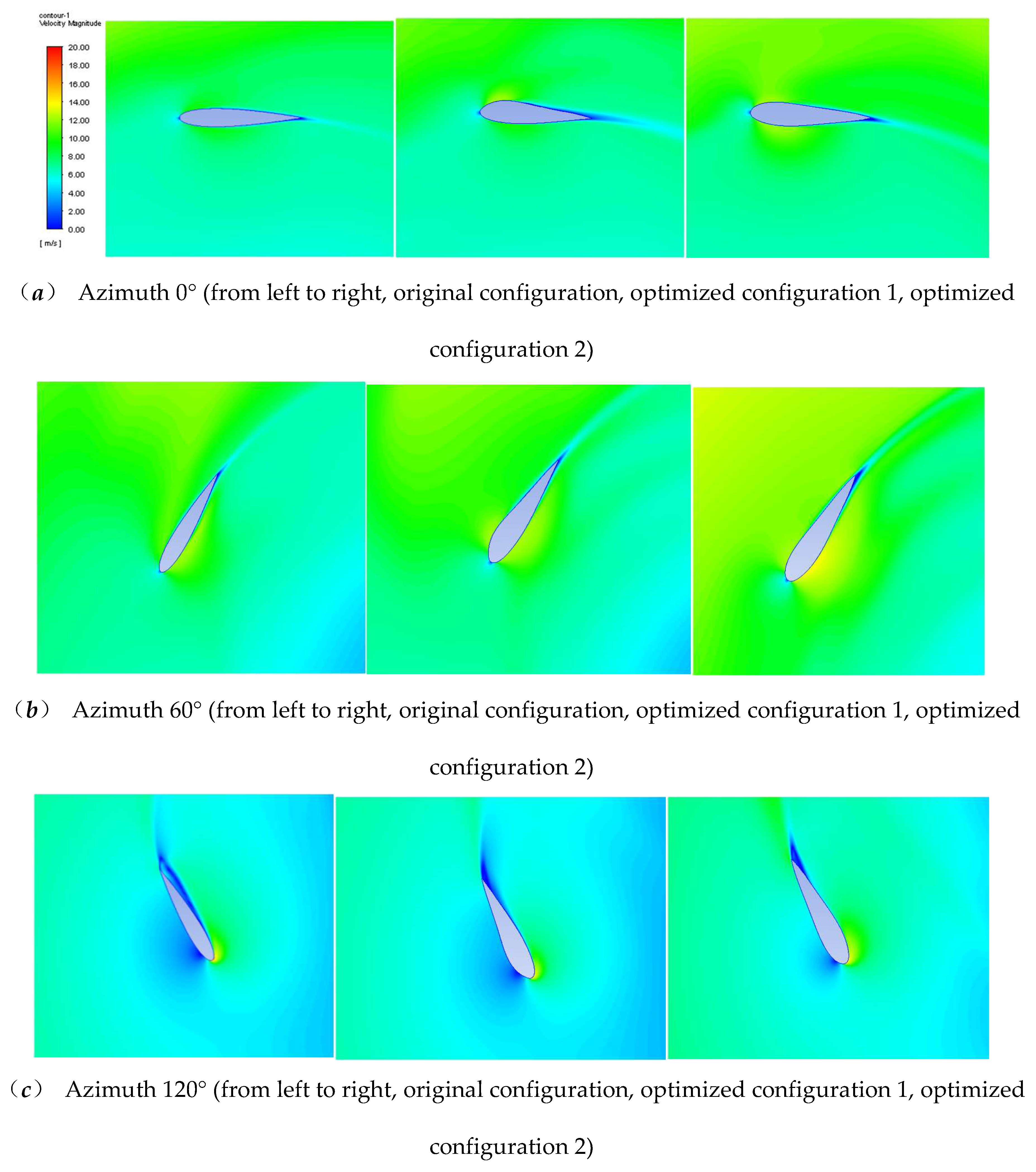
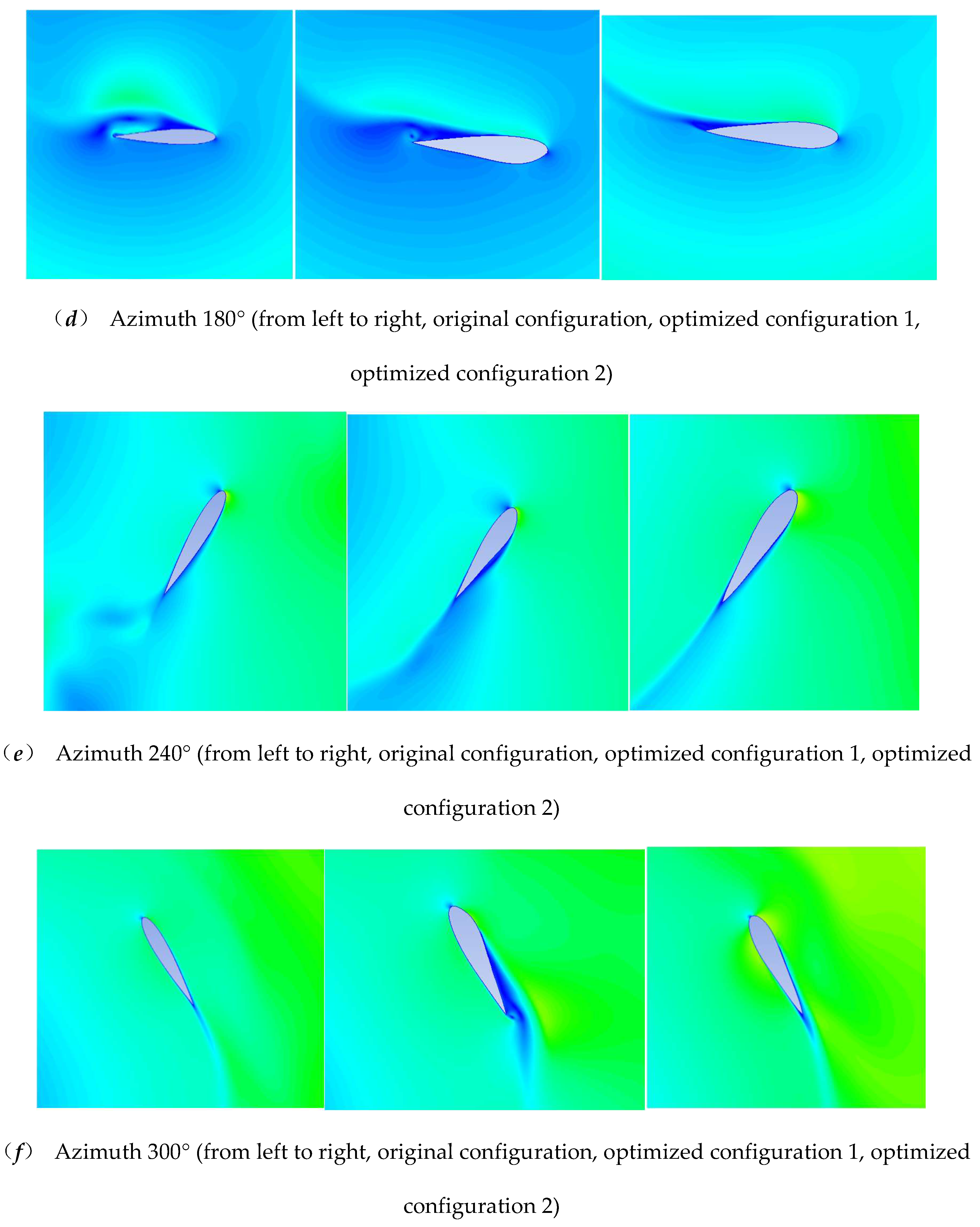

Table 2.
Time Step Irrelevance Verification Form.
| Degrees Of Rotation In A Single Step | Total Number of Steps | Total Number of Iterations | Time Step/s |
|---|---|---|---|
| 0.5° | 720 | 5760 | 0.0007272205 |
| 1° | 360 | 2880 | 0.001454441 |
| 2° | 180 | 1440 | 0.002908882 |
Table 3.
Optimized parameters for both configurations.
| Parameters | Original Configuration | Optimized Configuration 1 (Thickness Parameter Controlled Below 0.5) | Optimized Configuration 2 (Thickness Parameter Controlled Below 0.3) |
|---|---|---|---|
| a1 | 0.2117 | 0.2281 | 0.3 |
| a2 | 0.1963 | 0.44641 | 0.3 |
| a6 | 0.166 | 0.25401 | 0.29957 |
| b1 | -0.2117 | -0.27724 | -0.24763 |
| b2 | -0.1963 | -0.19033 | -0.26335 |
| b6 | -0.166 | -0.27971 | -0.29948 |
| mounting angle α | 0 | 3.5 | 1.1 |
| Power extraction factor Cp | 0.3127 | 0.3646 | 0.3491 |
Disclaimer/Publisher’s Note: The statements, opinions and data contained in all publications are solely those of the individual author(s) and contributor(s) and not of MDPI and/or the editor(s). MDPI and/or the editor(s) disclaim responsibility for any injury to people or property resulting from any ideas, methods, instructions or products referred to in the content. |
© 2025 by the authors. Licensee MDPI, Basel, Switzerland. This article is an open access article distributed under the terms and conditions of the Creative Commons Attribution (CC BY) license (http://creativecommons.org/licenses/by/4.0/).
Copyright: This open access article is published under a Creative Commons CC BY 4.0 license, which permit the free download, distribution, and reuse, provided that the author and preprint are cited in any reuse.


