
Submitted:
21 March 2025
Posted:
24 March 2025
You are already at the latest version
Abstract
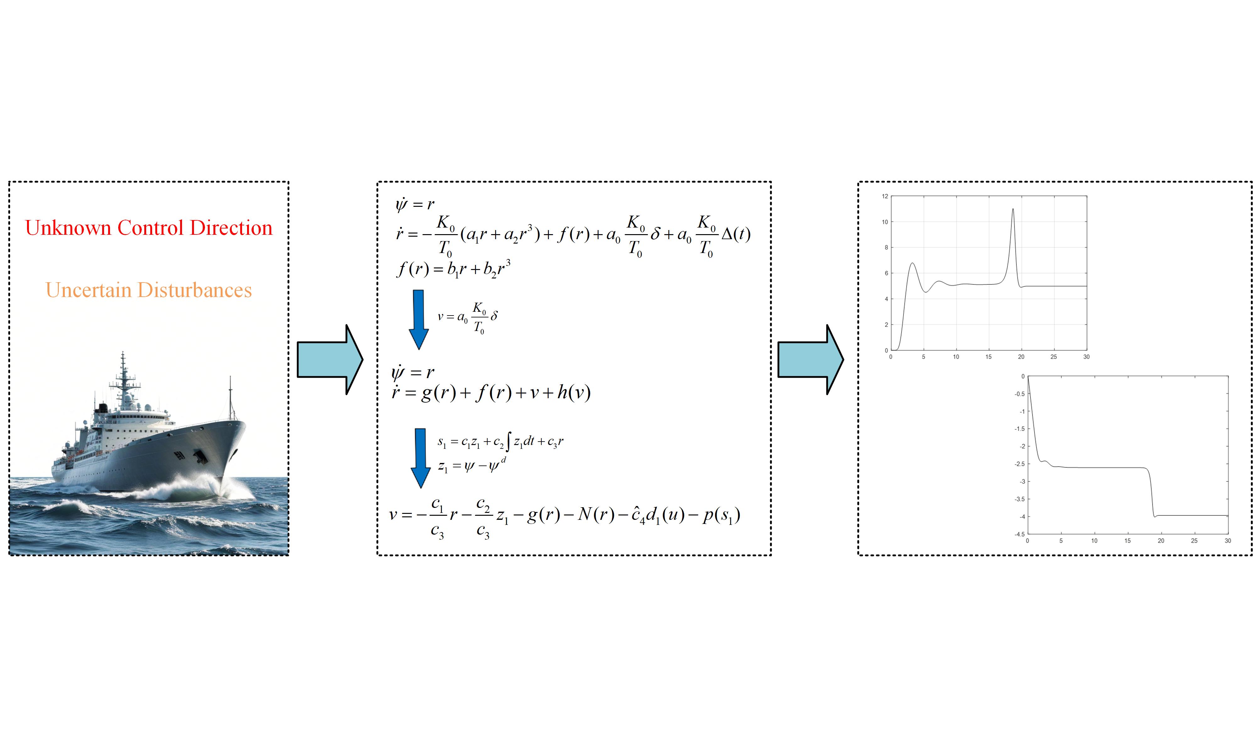
This paper focuses on the ship control system and studies the problem of unknown control direction. Considering that the traditional Nussbaum gain method has to consider the complex situation where the gain converges to both positive and negative infinity when proving the system stability, a unilateral Nussbaum function is defined in this paper. By constructing this function, the design and proof process of the adaptive Nussbaum gain method are simplified. Taking the ship course - keeping control system as the research object, a course angle tracking controller is designed by combining neural network, robust adaptive and sliding mode control techniques. A dual - input RBF single - output neural network is used to approximate the uncertain part of the system, and the robust adaptive control is adopted to deal with the unknown disturbance. The simulation results show that the proposed method can effectively cope with the problems of unknown control direction and its jump, keeping the system stable, which has great theoretical and engineering application value.
Keywords:
Nussbaum gain
; Sliding mode
; Ship Course keeping
; RBF network
; Unknown control direction
1. Introduction
In the field of control systems for complex dynamic systems, especially ship - related control, the design of controllers is a critical research area. The control direction [1,2] , which is a key factor, significantly affects the performance and stability of these systems.
For ship control systems, the ship course - keeping control system is a complex nonlinear system. It is influenced by multiple factors, including unknown control direction coefficients, uncertain parameters, and external disturbances. Traditional control methods often face challenges in achieving satisfactory control performance in such complex scenarios. Some early control strategies, although effective to a certain extent, failed to fully account for the complexity introduced by unknown control directions. For instance, they might have simplified the system model by assuming known control directions, which is far from the real - world situation where control directions can change due to various factors like sea conditions and ship - specific dynamics.
In the past two decades, the control problem of continuous nonlinear systems with unknown control directions has attracted the attention of many scholars. Currently, the main direction with numerous research achievements and breakthroughs is the Nussbaum gain adaptive control method [3,4]. The Nussbaum gain theory was first proposed by Nussbaum [5] in 1983, taking a simple first - order system as an example to illustrate that this theory can solve the control problem of systems with unknown high - frequency control coefficients.
There have been many studies on Nussbaum gain control for the problem of a single unknown control direction. For example, in 1998, Ye, X. [6] designed a controller for a lower - triangular system by combining backstepping design with the Nussbaum method. In 2003, Shuzhi Sam, G. [7] conducted research on adaptive control under the condition of insufficient prior knowledge of virtual control coefficients. In 2006, Zhou, Y. [8] designed a backstepping Nussbaum gain controller for systems with unknown high - frequency gain matrix signs. However, in the simulation, only the situation of unknown signs was considered, and the situation of high - frequency sign jumps was not taken into account. In 2009, Bechlioulis, C.P. [9] proposed a robust adaptive control algorithm for a class of uncertain nonlinear disturbed systems with virtual control gain functions of unknown signs. In 2012, Jin, K. [10] pointed out that when the control direction is unknown, the solution approach based on the Nussbaum function proposed by Nussbaum is of milestone significance in this field and remains the main method to solve the problem of unknown control directions to this day. In 2024, Liu, G.L. [11] a novel Nussbaum function design is proposed to address the coupling cancellation problem of traditional Nussbaum functions in multi unknown control direction stochastic systems, and the stability of the system is ensured through Lyapunov analysis. To reduce computational burden, an innovative combination of static composite event triggering mechanism (integrating tracking error and control signal triggering conditions) and intermittent feedback is proposed, and a dynamic composite triggering mechanism is further developed for optimization. The overall scheme significantly reduces the frequency of control updates while ensuring the boundedness of tracking errors.
However, the traditional Nussbaum gain method has its drawbacks. The traditional Nussbaum gain method has to consider the situation that the Nussbaum gain converge to both and , which is not very convinient for the proof of system stability. So in this paper we tries to constructed a new kind of Nussbaum function which maks it is easy to prove the stability of a control system.
The relationship between Mittag Leffler function and Nussbaum type function was discussed in [12]. It showed that the Mittag Leffler function can be turned into Nussbaum type function under some special conditions. The characteristics of Nussbaum type function were revealed and many new kinds of Nussbaum type functions were proposed. In this paper, a special Nussbaum type function, which is called unilateral Nussbaum function, is defined. It is used to design adaptive controller for nonlinear system, which can simplify the design and proof of adaptive Nussbaum gain method. It is necessary to analysis the situation that the Nussbaum gain converge to both and when the traditional Nussbaum gain method is used. But only the consideration of situation is necessary if the unilateral Nussbaum gain method is adopted. So it has better quality than traditional Nussbaum function.
When backstepping design method is applied to high-order systems, it is prone to the over-parameterization problem, which makes the design extremely complicated. Due to its excellent robustness and order reduction characteristics, sliding mode control [13,14] has been widely used in many engineering systems. In this paper, adaptive sliding mode control is also adopted to reduce the complexity of the controller design for high-order systems. Meanwhile, a method that combines sliding mode control with the Nussbaum gain is introduced to address the problem of unknown control direction. The over-parametirc problem was considered in [15], but the unknown control direction problem is neglected. So in this paper, the unilateral Nussbaum gain method is proposed and used in ship course keeping system with uncertainties and unknown control direction. Meanwhile, aiming at the special nonlinear problems of ship systems, a class of dedicated RBF neural networks [16,17,18,19] was designed. Sliding mode control was used to reduce the order of the system, and it was combined with the Nussbaum method to simplify the design and analysis process of traditional Nussbaum gain control. In this paper, we aim to address the research gaps in the existing literature.
We apply this new method to the ship course - keeping control system. Through theoretical analysis and simulations, we verify the effectiveness of the proposed method, offering a novel solution for ship control systems with unknown control directions in practical engineering applications. The innovative points of this article are as follows:
- Innovation point regarding neural network: Considering the special nonlinear and uncertain characteristics of the ship, a dedicated RBF nonlinear neural network has been designed. Its basis functions are a combination of linear and cubic terms, which can rapidly compensate for the uncertainties of the system.
- Innovation point regarding the unknown control direction: The large system with the problem of unknown control direction is decomposed into a two-dimensional situation. One dimension forms a new dynamic system with the sliding mode surface, while the other dimension is reserved for the stability analysis of the Nussbaum gain. The design for the problem of unknown control direction is divided into two steps, systematically constructing an analytical method for this type of problem, especially simplifying the proof.
2. Methodology
2.1. Unilateral Nussbaum Gain Control of Nonlinear System
To make the following introduction of a new Nussbaum gain method simple, we propose the definition of unilateral Nussbaum gain at first.
Definition 1:
A function is called a unilateral Nussbaum type function if it satisfies
Considering the traditional Nussbaum function, it is obvious that is not belonged to unilateral type Nussbaum function, and is belonged to unilateral type Nussbaum function.
The following lower triangular nonlinear system is used to illustrate the unilateral Nussbaum gain control method.
Considering the following N order SISO sysetem
where is the unknown control direction, , and define a new input variable as ,and design a sliding mode surface as
So the system can be rewritten as
Then the unknown control direction is not existed in the system equation.
Assumption 1:
There exist a control
and a Lyapunov function such that the above system satisfies and the system is stable.
Lemma 1:
For the above - mentioned system, if we design
and where is an unilateral Nussbaum gain function, then the above system is stable under the condition of unknown control direction.
The proof is as follows:
According to the Assumption 1, there exists a Lyapunov function
Solve the derivative of the Lyapunov function, we get
It also can be transformed as
Considering the control law , it is easy to get
Do the integral computation on both side of the inequality, we get
Design the adaptive regulation law as
We have
Then
Considering that , we get
Then use the below characteristic of unilateral Nussbaum gain function
And use apagoge ,we assume is unbounded, such as ,then we have
Then a contradiction appears and the above assumption does not satisfies and is bounded. It is easy to prove that all signals of the close system are bounded. With the help of Baralat lemma, we can prove that the system is stable.
2.2. Model of Ship Course Keeping Control System with Unknown Control Direction
The mathematical model of the ship course - keeping control system is as follows:
where is a unknown control direction coefficient, and are unknown coefficients, , , and are known coefficients of system . is unknown disturbance, which is bounded and , is the bounded function and it is known, is the yaw speed, is the heading angle. The control objective is to design rudder angle , such that to make the system stable and make the heading angle. Trace the desired value.
First, we design a new control variable as , then the above model can be rewritten as:
where , . At this point, there is no problem of unknown control direction in the system since is completely known, and the uncertainties of the model mainly focus on and . Next, the adaptive sliding mode control method is adopted to design to make the above system stable.
2.3. Nueral RBF Network and Sliding Mode Control for Ship Course - Keeping Control System Without Unknown Control Direction
Firstly, the ship course angle command is set as , and the course angle error variable is defined as
A proportional - integral - derivative (PID) type sliding mode surface is selected as
The derivative of the sliding mode surface is obtained as
Since the structure of the part is known, but only its parameters are uncertain, a special RBF neural network with a combination of cubic and linear terms is designed according to the characteristics of the above - mentioned model to approximate the uncertain part of the system. And robust adaptive control will be used to deal with .
The designed dual - input RBF single - output neural network is as follows
where and are the weights of the neural network, is the output of the neural network, and the basis functions of the neural network are defined as
The role of the basis functions is mainly to automatically adjust the influence of the weights according to the values of the sliding mode surface and the error, so as to achieve the approximation of the uncertain part ,,,, are parameters of RBF network.
According to the result of the derivative of the sliding mode surface, the control law is designed in a back - stepping manner as follows
where .
where is an odd integer and is a softening coefficient. It is not difficult to prove that
where , and are constant control parameters.
After further arrangement, we get
Substituting it into the derivative formula of the sliding mode surface, we get
Due to the approximation characteristics of the neural network, and because the structure of the neural network in this paper is consistent with the structure of the uncertain part of the system, there obviously exist optimal neural network weights and such that
where is an arbitrarily small positive number. In fact, when the following equations are satisfied
It can be obtained that the optimal neural network weights and will ensure that
At this time
The weight error of the neural network is defined as follows
Then
At this time
First, considering the derivative of the weight error of the neural network, due to the constant - value characteristics of the optimal neural network weightsand , we have
In order to use the neural network to eliminate the uncertainty , the weight adaptation law of the special RBF neural network with a combination of cubic and linear terms is designed as follows
At this time, if the Lyapunov function related to the neural network weights is selected as
The derivative of it is obtained as
After further arrangement, we get
Thus, we have
The above design mainly uses the neural network to eliminate the uncertain part . Next, a robust adaptive control is designed to deal with .
2.4. Robust Control for Uncertainties of Ship Course - Keeping Control System with Unknown Control Direction
Considering the uncetainties of ship course keeping control system that , we have
After further arrangement, we get
At this time, define
Define: ,At this time, its derivative is obtained as
Therefore, the adaptive parameter adjustment law can be designed as
The estimation error of the unknown parameter is defined as
At this time, the Lyapunov function related to the parameter is selected as
The derivative of it is obtained as
At this time, considering that the sign change only brings a momentary disturbance to the system, it is approximately considered that
The Lyapunov function related to the sliding mode surface is selected as
The derivative of it is obtained as
So far, the total Lyapunov function of the system is selected as
Using the control law designed as shown in the formula , its derivative is obtained as
According to the Lyapunov stability theory, it is not difficult to prove that the system is stable, all signals are bounded, and thus the sliding - mode surface variable converges to 0. Since the coefficients , and are positive and Hurwitz when the sliding - mode surface variable is selected as , it is not difficult to further prove that the error state is stable, that is, approaches 0, so as to achieve the control goal of tracking the heading angle.
According to the above lemma 1, we can directly design and , at this time, in Assumption 1 is set as . Then, based on the above lemma, it is not difficult to prove that the above design can ensure the stability of our ship course - keeping system and the tracking of the heading angle.
After establishing the theoretical framework, the following section presents an example and simulation to verify the effectiveness of the proposed method.
3. Results and Discussion
3.1. Example
For the above - mentioned model, the parameter selection is as follows: ,,,;The ship course angle command is selected as ,and design
And choose the unilateral Nussbaum gain function as
3.2. Simulation Results and Discussion
When the unknown control direction is not taken into account,the we set . At this time, the control effects are shown in Figure 1 and Figure 2 below. Figure 1 is the yaw angle response curve of the ship, and Figure 2 is the yaw angle rate response curve. As shown in Figure 1 and Figure 2, the system response is relatively smooth, and the overshoot is small. Since the unknown control direction is not considered, the magnitude of the control gain can be reasonably selected, enabling the response curve of the entire system to have excellent dynamic performance. However, when the control direction is unknown, especially when a jump occurs, the difficulty of control will increase sharply. In particular, due to the unknown jump of the control direction, which is an unmeasurable and unpredictable jump, the system is likely to switch from negative feedback to positive feedback, resulting in a transient divergence phenomenon, thereby increasing the difficulty of control.
However, considering the possible problem of unknown control direction in practical situations, we set ,As shown in Figure 6, the search jump situation of the Nussbaum gain at this time is shown in Figure 5. The yaw angle rate response curve under the condition of control direction jump is shown in Figure 4, and the yaw angle response curve is shown in Figure 3.It can be seen from Figure 5 that the jump of the Nussbaum gain can quickly search following the jump of the control direction. From Figure 3 and Figure 4, it can be observed that due to the drastic challenges brought to the system by the jump of the control direction, the control method proposed in this paper can automatically adjust, find the appropriate control gain direction for compensation again, so that the overall gain direction of the system remains unchanged, thus keeping the system stable.
From the simulation results, the rationality and effectiveness of the method proposed in this paper are verified. It can solve the huge challenges to the system stability caused by the sharp gain jumps in practical engineering, which endows the method proposed in this paper with high theoretical value and practical engineering value.
4. Conclusions
For the complex nonlinear dynamic model of the ship maneuvering system, a course angle tracking controller that combines neural networks, robust adaptive control, and sliding mode control has been designed. Moreover, the problem of unknown control direction has been taken into account, and a unilateral Nussbaum gain control function has been introduced to address it. The final simulation also demonstrates the effectiveness of the method proposed in this paper.
The main innovations and contributions of this paper are as follows. First, the large system with the problem of unknown control direction is decomposed into a two-dimensional situation. One dimension forms a new dynamic system with the sliding mode surface, while the other dimension is reserved for the stability analysis of the Nussbaum gain. Therefore, the design for the problem of unknown control direction is divided into two steps, systematically constructing an analytical method for this type of problem, especially simplifying the proof.Second, the unilateral Nussbaum gain method is combined with the sliding mode control method and applied to the control of the ship system. As a result, both the problem of unknown direction and the over-parameterization problem in the backstepping design are solved.Third, considering the special nonlinear and uncertain characteristics of the ship, a dedicated RBF nonlinear neural network has been designed. Its basis functions are a combination of linear and cubic terms, enabling rapid compensation for the uncertainties of the system.
Author Contributions
Guoxin Ma: Conceptualization, methodology, formal analysis, project man- agement, funding acquisition, paper framework; Dongliang Li: Methodology derivation, simulation experiments, paper writing and editing; Qiang Wei: Investigation, formal analysis, data organiza- tion, and funding acquisition; Lei Song: Paper verification and supervision.
Funding
This work is supported by the National Key R&D Program of China (Grant No. 2021YFE0111600).
Data Availability Statement
When using the data in this manuscript, readers can directly cite this manuscript or contact the authors for access.
Acknowledgments
This study would like to express special gratitude to the National Key Research and Development Program (2021YFE0111600) for its funding.
Conflicts of Interest
The authors declare no conflicts of interest.
References
- Feng, X.; Wang, C. Adaptive tracking control-based Nussbaum gain for a class of multi-input and multi-output nonlinear systems with time-varying state constraints. Proc. Inst. Mech. Eng. Part I-J Syst Control Eng. 2024, 238, 1153–1165. [Google Scholar]
- Mousavi, A.; Markazi, A.H.D. Adaptive fuzzy sliding-mode control of under-actuated systems with unknown input gain function. Proc. Inst. Mech. Eng. Part C-J. Eng. Mech. Eng. Sci. 2024, 238, 5455–5468. [Google Scholar]
- Ding, J.; He, X.; Wu, L.; Yu, Q. Nussbaum gain adaptive fuzzy control for switched nonlinear systems with predefined output and full time-varying states constraints. Asian J. Control 2023, 26, 175–189. [Google Scholar]
- Miao, B.; Li, S.; Liu, L. Nussbaum gain adaptive control for full-state constrained cyber-physical system under network attacks and actuator failures. Int. J. Robust Nonlinear Control 2023, 34, 2515–2531. [Google Scholar] [CrossRef]
- Nussbaum, R.D. Some remarks on a conjecture in parameter adaptive control. Syst. Control Lett. 1983, 3, 243–246. [Google Scholar] [CrossRef]
- Ye, X.; Jiang, J. Adaptive nonlinear design without a priori knowledge of control directions. IEEE Trans. Autom. Control 1998, 43, 1617–1621. [Google Scholar]
- Shuzhi Sam, G.; Wang, J. Robust adaptive tracking for time-varying uncertain nonlinear systems with unknown control coefficients. IEEE Trans. Autom. Control 2003, 48, 1463–1469. [Google Scholar] [CrossRef]
- Zhou, Y. Output - feedback adaptive control for MIMO uncertain nonlinear systems. Doctoral dissertation, Southeast University, Jiangsu, China, 2006.
- Bechlioulis, C.P.; Rovithakis, G.A. Adaptive control with guaranteed transient and steady state tracking error bounds for strict feedback systems. Automatica 2009, 45, 532–538. [Google Scholar]
- Jin, K.; Sun, M.X. Adaptive repetitive control for nonlinear systems with unknown control directions. Contr. Theory Appl. 2012, 29, 1176–1180. [Google Scholar]
- Liu, G.L.; Yang, Y.L.; Ding, D.W.; Li, Q. Adaptive Nussbaum design using composite triggering condition for stochastic nonlinear systems with multiple unknown control directions. Int. J. Robust Nonlinear Control 2024, 34, 11487–11512. [Google Scholar] [CrossRef]
- Li, Y.; Chen, Y. When is a Mittag–Leffler function a Nussbaum function? Automatica 2009, 45, 1957–1959. [Google Scholar] [CrossRef]
- Dang, S.T.; Dinh, X.M.; Kim, T.D.; Xuan, H.L.; Ha, M.H. Adaptive Backstepping Hierarchical Sliding Mode Control for 3-Wheeled Mobile Robots Based on RBF Neural Networks. Electronics 2023, 12, 2345. [Google Scholar] [CrossRef]
- Jiang, B.; Liu, D.; Karimi, H.R.; Li, B. RBF Neural Network Sliding Mode Control for Passification of Nonlinear Time-Varying Delay Systems with Application to Offshore Cranes. Sensors 2022, 22, 5253. [Google Scholar] [CrossRef] [PubMed]
- Kim, S.-H.; Kim, Y.-S.; Song, C. A robust adaptive nonlinear control approach to missile autopilot design. Control Eng. Practice 2004, 12, 149–154. [Google Scholar] [CrossRef]
- Zhou, Y.N.; Sun, Z.K. Control of stability in semi-passive robot based on RBF neural network. Chaos Solitons Fractals 2023, 173, 113623. [Google Scholar] [CrossRef]
- He, Y.; Zhou, Y.; Cai, Y.; Yuan, C.; Shen, J. DSC-based RBF neural network control for nonlinear time-delay systems with time-varying full state constraints. ISA Trans. 2022, 129, 79–90. [Google Scholar] [CrossRef] [PubMed]
- Li, T.S.; Duan, S.K.; Liu, J.; Wang, L.D. An improved design of RBF neural network control algorithm based on spintronic memristor crossbar array. Neural Comput. Appl. 2018, 30, 1939–1946. [Google Scholar]
- Addeh, A.; Khormali, A.; Golilarz, N.A. Control chart pattern recognition using RBF neural network with new training algorithm and practical features. ISA Trans. 2018, 79, 202–216. [Google Scholar] [CrossRef] [PubMed]
Figure 1.
Yaw angle response curve.
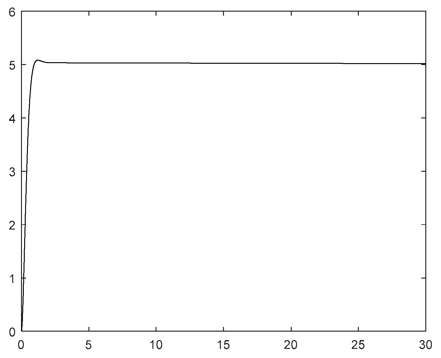
Figure 2.
Yaw angle rate response curve.
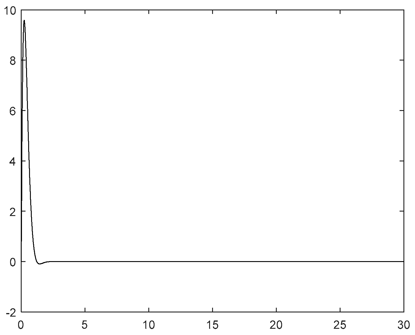
Figure 3.
The yaw angle response curve under the condition of control direction jump.
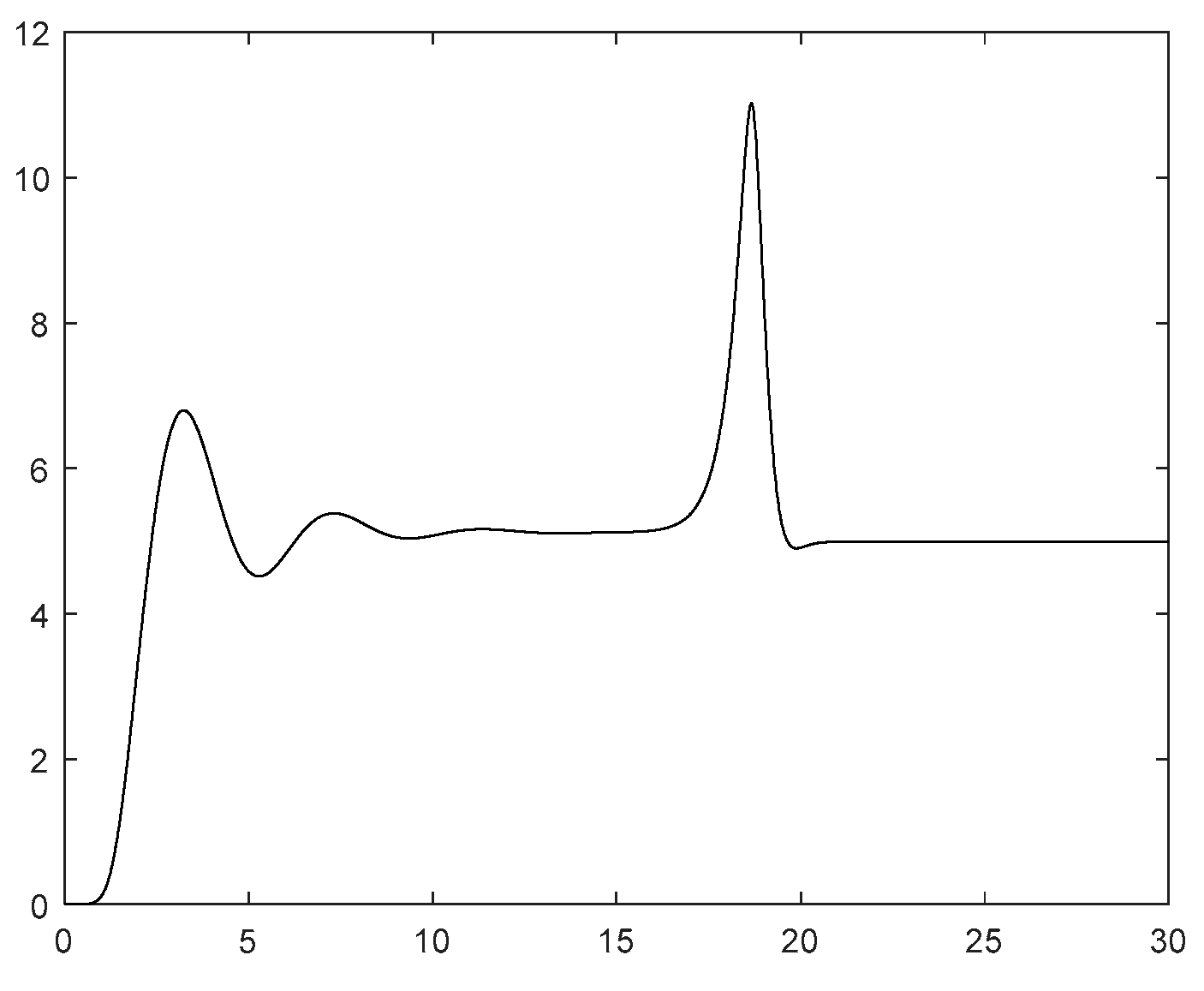
Figure 4.
The yaw angle rate response curve under the condition of control direction jump.
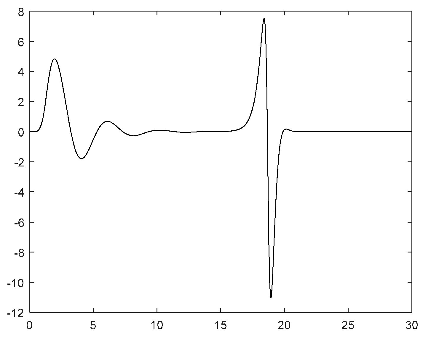
Figure 5.
The jump curve graph of the Nussbaum Gain.
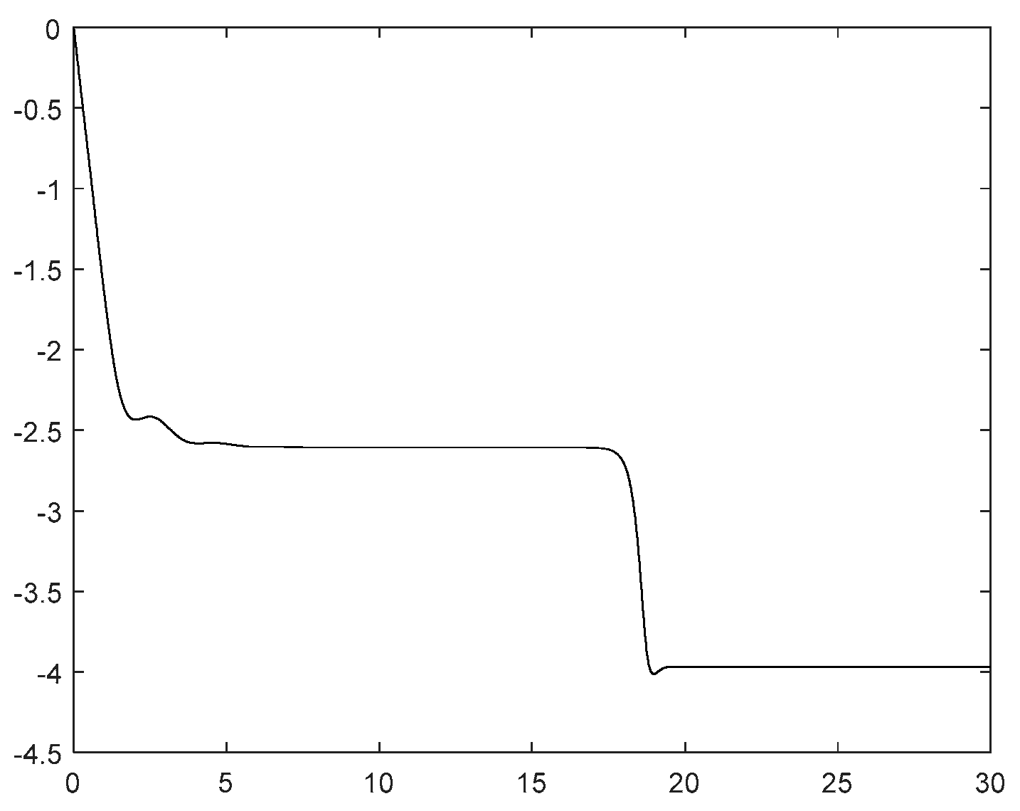
Figure 6.
The jump curve graph of the control direction.
Disclaimer/Publisher’s Note: The statements, opinions and data contained in all publications are solely those of the individual author(s) and contributor(s) and not of MDPI and/or the editor(s). MDPI and/or the editor(s) disclaim responsibility for any injury to people or property resulting from any ideas, methods, instructions or products referred to in the content. |
© 2025 by the authors. Licensee MDPI, Basel, Switzerland. This article is an open access article distributed under the terms and conditions of the Creative Commons Attribution (CC BY) license (http://creativecommons.org/licenses/by/4.0/).
Copyright: This open access article is published under a Creative Commons CC BY 4.0 license, which permit the free download, distribution, and reuse, provided that the author and preprint are cited in any reuse.


