Submitted:
20 March 2025
Posted:
21 March 2025
You are already at the latest version
Abstract
The heat transfer coefficient or the HTC is an industry-standard indicator of building energy performance. It has been predicated on an assumption that it is of a constant value, and several different methods have been developed to measure and calculate the HTC as a constant. Whilst there are limited variations of results obtained from these different methods, none of these methods consider a possibility that the HTC could be dynamically variable. Our experimental work shows that the HTC is not a constant. Experimental evidence base from our environmental chambers, which contain detached houses, and in which ambient air temperature can be controlled between -20 °C and +40 °C, with additional relative humidity control and with weather rigs that can introduce solar radiation, rain and snow, shows that the HTC is dynamically variable. Analysis of data from fully instrumented and monitored houses in a combination with calibrated simulation models and data processing scripts based on genetic algorithm optimization provide experimental evidence of dynamic variability of the HTC. This research increases the understanding of building physics properties and has a potential to change the way the heat transfer coefficient is used in building performance analysis.
Keywords:
Heat transfer coefficient (HTC)
; thermal diffusivity
; time constant
; energy performance
; dynamic variability
; experimental evidence
; building physics
; environmental chambers
; genetic algorithm
; machine learning
; simulation models
1. Introduction
The heat transfer coefficient (HTC) is an industry-standard indicator of building energy performance. International Standard ISO 13789 [1] defines the heat loss coefficient as the “Sum of transmission and ventilation heat loss coefficient”, where transmission heat loss coefficient is defined as “Heat flow rate from the heated space to the external environment by transmission divided by the temperature difference between internal and external environments” and ventilation heat loss coefficient is defined as “Heat flow rate from the heated space to the external environment by ventilation divided by the temperature difference between internal and external environments.”
Whilst the above definition provides the scope for dynamic variability, a widely adopted approach in industry is that the HTC is a constant, and several methods have been developed to measure it and calculate it as a constant. Although there are limited variations in the results from these methods, none consider the possibility that the HTC could be dynamically variable.
Our experimental work shows that the HTC is not a constant. We conducted experiments in Environmental Chamber of Energy House 2.0, with one of two detached houses, where we controlled ambient air temperature between -20 °C and +40 °C, relative humidity, and introduced weather conditions like solar radiation, rain, and snow. These experiments provided evidence of the HTC’s dynamic variability.
Analysis of data from a fully instrumented and monitored house, combined with calibrated simulation models and data processing scripts based on genetic algorithm optimization provides evidence that supports the dynamic variability of the HTC.
1.1. The Current State of the Research Field
In his doctoral thesis, Eastwood [2] investigated the HTC variability in dwellings influenced by the boundary conditions, including the measurement accuracy of indoor air temperature, outdoor air temperature, internal heat gains, wind speed and infiltration and ventilation heat loss, party wall heat transfer, ground floor heat transfer, loses to adjacent dwellings or unoccupied spaces and estimates of solar gains. The work aimed to improve the accuracy of measuring thermal performance of dwellings. Out of circa 30 dwellings measured, the HTC variation was between 202.5 W/K and 208.8 W/K for in-use HTC and between 197.5 W/K and 199.9 W/K for co-heating HTC. This variability is therefore attributed to measurement errors rather than to the variability of the HTC itself.
A limited variability of the HTC has been attributed to different measurement methods, such as in use HTC versus a co-heating HTC, as well as to the circumstances during the tests and instrumentation accuracy [3].
Sougkakis and co-authors [4] studied the suitability of a QUB (Quick U-value of Buildings) method to create ‘consistent and robust estimates’ of the HTC. In 147 tests of a detached house at the University of Nottingham, they found that over 95% of the results were within ±15% from the mean value. In other words, the intention was to demonstrate consistency with a constant value.
In a similar study of the QUB method, Ahmad and co-workers [5] found that a simulation of QUB experiments during the winter months were within ±15% of the steady state HTC.
Juric and co-authors studied the Sereine method, [6] a dynamic in-situ test method for determining a dwelling’s heat transfer coefficient (HTC) and transmission heat transfer rate (HTR). It applies a pseudo-random heating pattern to an unoccupied house, using external temperature and heating power as inputs to an RC model selected via the Bayesian Information Criterion. The method controls solar gains, seals ventilation, and accounts for external conditions through an equivalent temperature approach. Validation includes a field study at the French National Solar Energy Institute, where results aligned with a coheating test within uncertainty limits and EnergyPlus simulations across 21 French locations, showing seasonal variations and higher uncertainty for externally insulated buildings. Test durations range was from 24–96 hours, with a recommended minimum of 24–72 hours depending on archetype and climate.
Vighio and co-authors [7] worked on experimental measurement and theoretical validation of an ‘Overall Thermal Transfer Value’ or OTTV in W/m2, using and Eco-Home Case Study Building. They recorded daily fluctuation of the OTTV, approximately between -30 W/m2 and +180 W/m2 for 30 days in September 2023. They also developed an OTTV equation and found a strong linear correlation between the equation generated values and values generated by EQUEST simulation engine. The authors’ home country Malaysia, together with Pakistan, Sri Lanka, Hong Kong, Thailand, and Singapore, have incorporated the OTTV in their building regulations. Although the OTTV is different from the HTC, both are indicators of building energy performance, where the OTTV is a variable and the HTC is deemed to be constant.
Industry stakeholders recognize the challenge of accurately characterizing building performance, though commercial sensitivity limits available literature on in-use heat transfer coefficient (HTC) measurement methods. The SMETER TEST project provides the most comprehensive comparison of commercial methodologies, evaluating eight SMETER technologies in a 30-home UK field trial [8]. Among these, Build Test Solutions’ Smart HTC underwent validation against coheating tests, showing <1% deviation and <4% repeatability variation over a minimum 21-day monitoring period [9]. Some industry methods, such as HomeLink’s “Time to Lose 1°C” (TTL) [10], measure related heat loss characteristics rather than the HTC directly.
1.2. Measuring and Modelling the HTC
Fitton [11] reported significant variations in the HTC measurements carried out using the same experimental setups. Twelve methods have been developed to measure the HTC, including the Coheating test, QUB (quick U value of Buildings), ISABELE, PSTAR/STEM, and others, where all of these methods measure the HTC as a constant, with typical expected errors between 3% and 30% [11].
The HTC of domestic buildings is commonly measured using the coheating (aggregate heat loss) test method [12,13]. This test involves heating the internal spaces of an unoccupied building to an elevated, stable temperature (typically around 21 °C), while measuring the electrical heat input required to maintain this temperature over a set period (typically two to three weeks). By plotting the daily heat input against the internal and external temperature difference (ΔT), the total heat loss (fabric and infiltration) can be quantified. Marshall et al. applied coheating tests under controlled conditions, demonstrating precise HTC measurements and emphasizing the value of controlled testing to accurately assess building fabric performance [14]. Farmer et al. also used coheating tests to quantify incremental improvements in the HTC through staged retrofits of a solid-wall Victorian dwelling, highlighting the effectiveness of the method for evaluating thermal impacts of retrofit interventions [15]. Additionally, Jack et al. validated the reliability of coheating tests by demonstrating consistency (±10%) in the HTC measurements across multiple independent tests, confirming the robustness of this method [16].
The HTC predictions can also be modeled using steady-state methods such as the Standard Assessment Procedure (SAP), or dynamic thermal simulation (DTS) tools like DesignBuilder [17,18]. SAP employs a bottom-up approach, aggregating fabric and infiltration heat loss, whereas DTS tools simulate aggregate heat loss dynamically at hourly intervals. Johnston et al. presented empirical data from 38 coheating tests conducted on 25 distinct dwellings, all complying with the UK’s Building Regulations Part L1A 2006. The authors utilized these coheating tests to obtain measured HTC, providing valuable insights into the fabric performance of dwellings built to contemporary regulatory standards [19]. Parker et al. demonstrated the value of calibrating DTS models against the HTC data from coheating tests in retrofitted solid-wall dwellings, significantly improving model accuracy and enhancing retrofit decision making [20].
Fitton et al. evaluated rapid commercial methods for measuring the HTC against the traditional coheating test [21]. Saint-Gobain’s QUB [4,22] and the Veritherm method [23] both performed dynamic HTC measurements of unoccupied dwellings over a single night, considerably shorter than the duration typically required for coheating tests. Both methods involve a dynamic protocol comprising an initial stabilization period at constant internal temperature, followed by a heating period with constant power input, and ending with a free cooling phase. Each method relies on assumptions about fabric performance to estimate the required power input, and both utilize integrated hardware and software to control internal conditions, measure power input, and analyze the collected data. A key difference in equipment between the methods is that Veritherm uses air circulation fans during testing, whereas QUB does not. The results show that, when measurement uncertainty is considered, HTC values from these alternative methods generally align with those obtained from the coheating test. However, Veritherm’s measurement uncertainty is up to twice that of QUB. Additionally, the HTC measurements from QUB are approximately 15% lower than those from the coheating test, whereas the Veritherm results are about 6% lower. The results are summarized in Table 1 [21].
1.3. The Knowledge Gap
Whilst the above is by no means an exhaustive account of the state of the research field, a clear knowledge gap is beginning to emerge. The HTC is generally deemed to be constant, with limited variability due to specific test conditions and measurement uncertainties, as corroborated by the results in Table 1. It also appears that the HTC has always been calculated from carefully planned test data. In the remainder of the paper, we will explain how the HTC relates to fundamental physics properties of materials and introduce experimental evidence of its variability that is well beyond the measurement discrepancies and uncertainties. We will also demonstrate how the HTC can be ‘reverse-engineered’ from data from an ongoing monitoring of a building, without any preconditioning or other preparations of the building.
2. Materials and Methods
2.1. Linking the HTC to Dynamic Heat Transfer in a Building
In this section we will establish the link between the HTC and fundamental physics properties of a building.
The overall heat loss from a building is calculated as follows [24]:
where
Q—overall heat loss rate (W)
HTC—heat transfer coefficient (W/K
Ti—internal air temperature (K)
To—external air temperature (K).
The heat transfer coefficient consists of the following components
where
Hc—conductive heat loss coefficient (W/K)
Htb—thermal bridging heat loss coefficient (W/K)
Hv—ventilation and infiltration heat loss coefficient (W/K).
Each of the components of the HTC is defined further below. The conductive heat loss coefficient is defined as:
where
Hc—conductive heat loss coefficient (W/K)
Ui—thermal conductance of the i-th building element (W/(m²K))
Ai—surface area of the i-th building element (m²)
n—number of building elements.
The thermal bridging heat loss coefficient is defined as
where
Htb—thermal bridging heat loss coefficient (W/K)
Li—length of the i-th linear thermal bridge (m)
Ψi—linear thermal transmittance of the i-th thermal bridge (W/(m∙K))
The ventilation and infiltration heat loss coefficient is defined as
where
Hv—ventilation and infiltration heat loss coefficient (W/K)
N—volume air change per hour (h⁻¹)
V—building volume (m3).
The only building materials property is in Equation (3), contained in the transmittance of the wall (the U-value), is thermal conductivity:
where
d—wall thickness in meters (m)
k—thermal conductivity in W/(m∙K).
For a multilayered wall, resistances of all layers are added together to obtain the total resistance:
where
Ri—internal surface resistance
Ro—external surface resistance
R1, R2, R3…—resistances of individual construction layers
and thermal transmittance (the U-value) is then calculated as the inverse of thermal resistance for each individual building component:
Thermal conductivity is the only physics property in Equations (1-5). As thermal conductivity does not change, Equations (1-5) represent steady state building heat transfer.
However, the heat diffusion equation developed by Fourier [25,26] uses thermal diffusivity for dynamic heat transfer, instead of a single physics parameter for steady state heat transfer:
where
T—temperature (K)
—heat flux (W/m2)
k—thermal conductivity in W/(m∙K)
α—thermal diffusivity (m2/s)
t—time (s)
and where thermal diffusivity is defined as
where
k—thermal conductivity in W/(m∙K)
ρ—density (kg/m3)
c—specific heat (J/(kg∙K)).
Representation of building heat transfer using thermal diffusivity, with three physics properties of materials (conductivity, density and specific heat) corresponds much closer to the dynamic processes in buildings, instead of using a steady state approach with a single physics property of materials (conductivity) in Equations (1-5). But how can thermal diffusivity be used to represent heat transfer of a specific building?
This is explained using the approach developed on the basis of a simplified heat balance equation [24]:
where
C—effective thermal capacitance in MJ/K
Qloss—heat gain from solar radiation (W)
Qsol—heat gain from solar radiation (W)
Qint—internal heat gain in the building arising from heating or from casual gains (W).
Equation (11) can be rearranged as
where
Troom—difference between room temperature and the initial room temperature Tr—Tr,0
Tamb—difference between ambient air temperature and the initial room temperature Ta—Tr,0.
The solution of differential Equation (12) can be expressed as:
This can be rewritten as:
where time constant is defined as
The time constant represents the time it takes to go through 63% of the change from an initial event, such as heating on time, to the final equilibrium state. The effective thermal capacitance is:
where
m—mass (kg)
V—volume (m3)
c—specific heat (J/(kg∙K))
As the HTC is proportional to thermal conductivity k (HTC ∝ B k) where B is the proportionality constant, the time constant can be expressed as
where
α—thermal diffusivity (m2/s)
z—proportionality constant that represents the relationship B/V.
Equation (14) can now be rewritten as
that links thermal diffusivity α with a simple dynamic temperature equation for a building.
The material introduced in this section will facilitate our experimental investigation in the ‘Experiments and results’ section.
2.2. The Test Facility
This research is carried out under controlled conditions in Energy House 2.0 (Figure 1), and it uses experimental data from eHome2 (Figure 2) by Saint-Gobain Barratt constructed inside Environmental Chamber 1 in Energy House 2.0.
Energy House 2.0 is a globally unique building performance test facility. Constructed to allow for full-scale testing of structures under a controlled range of climatic conditions, the facility comprises two large chambers, capable of accommodating four family homes, two in each chamber. These chambers feature soil-filled pits, 1200 mm deep, isolated from the ground beneath and surrounding the pit by insulation. The walls and ceilings of each chamber are also insulated, providing isolation from the external climate and ensuring high levels of airtightness.
Each chamber is independently conditioned by a large heating, ventilation, and air conditioning (HVAC) system. Additionally, weather rigs are deployed to provide further climatic effects. These rigs control the climate within the chambers by manipulating various factors, such as temperature, humidity, and wind speed, as follows:
- Temperature: (-20 °C to 40 °C)
- Relative Humidity (20% to 90%)
- Wind (up to ~17 m/s)
- Rain (up to 200 mm/h)
- Solar Radiation (up to 1200 W/m2)
- Snow (up to 250 mm per day)
Temperature and relative humidity can be held at constant steady state or varied in seasonal or daily patterns.
2.3. The Test Building—eHome2
eHome2, by Saint-Gobain & Barratt Developments (Figure 2), is a 3-bedroom detached home built using closed panel timber frame construction, insulated with mineral wool. It is cladded externally with a proprietary brick slip system and render [21]. The house has an insulated concrete floor structure, double glazed windows and patio doors and a roof insulated with 400 mm of mineral wool insulation. The house is heated by a Valliant air source heat pump, which also supplies domestic hot water.
2.4. Simulation Models
A simulation model of eHome2 was initially created in DesignBuilder [18] (Figure 3) and exported into EnergyPlus [28] in order to enable the creation of a custom schedule for dynamic heating and cooling, with details in Figure 4
The meaning of the schedule in 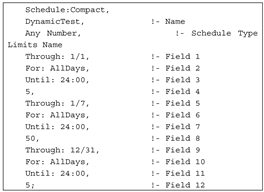 is that the building internal air temperature is kept at 5 °C over the first 24 hours of the simulation, where ‘1/1’ denotes ‘month/day’, and then for the next seven days, until day 7 of month 1 the target temperature is set to 50 °C, and after that it is set back to 5 °C again for the rest of the simulation year. The text after the exclamation symbol on every line represent comments.
is that the building internal air temperature is kept at 5 °C over the first 24 hours of the simulation, where ‘1/1’ denotes ‘month/day’, and then for the next seven days, until day 7 of month 1 the target temperature is set to 50 °C, and after that it is set back to 5 °C again for the rest of the simulation year. The text after the exclamation symbol on every line represent comments.2.3. Monitored Data
The following variables were monitored a one-minute time interval:
-
eHome2:
- Air temperature in seven points in each room
- Operative temperature in seven points in each room
- Relative humidity in the geometric center of each room
- Electrical energy consumption
- Heat meter output on ASHP primary flow and return
- Electrical energy consumption by circuit and by individual power outlet
-
Chamber:
- Air temperature at 36 points
- Relative humidity at 36 points
- Sub soil temperature under the center of each house
Chamber Sensor Locations are shown in Figure 5.
Whole house sensor locations and heat emitters in eHome2 are shown in Figure 6.
The experiments reported in this article are based on measurements obtained using the equipment listed in Table 4. Measurements were recorded at one-minute intervals by the Energy House 2.0 monitoring system.
2.5. Machine Learning of the HTC Using Measured Data
Machine learning of the HTC was carried out using the whole house temperature, the chamber temperature and the heat input from the heat input from the heating system. As there are 53 temperatures measured in the house, a simplified whole house temperature was calculated as follows:
where
Ti—middle shielded room temperature for each individual zone (°C)
Ai—floor area of each individual zone (m2)
i—individual zone index as in Table 5.
The machine learning of the HTC is based on a rearranged Equation (14):
As internal heat input Qint, solar input Qsol and temperature the outdoor-indoor temperature difference can influence the building slightly differently from their measured values, measurement scaling w1, w2 and w3 factors are introduced into Equation (20) as follows:
In this case, Qsol was set to zero, to correspond to the controlled conditions in Energy House 2.0 Environmental Chamber 1.
The machine learning of the HTC is based on setting up a fitness function as a root mean squared error between the internal room temperature calculated using Equation (21) and the measured internal room temperature calculated using Equation (19). The genetic algorithm was then used to evolve values of HTC, tc, w1, w2 and w3 to minimize the fitness function. This is done on a day-by-day basis, using the measured values recorded at one-minute interval and averaged to ten-minute intervals prior to starting the learning process.
The machine learning was implemented as a bespoke algorithm in Java programming language, where the input data stream consisted of monitored data and the output data stream consisted of the HTC and the RMSE. The elapsed time for processing of 140 days of data at ten-minute timestep lasted 0.23 seconds and of 12 days of data at ten-minute timestep lasted 0.13 seconds on an Apple MacBook Pro with Apple M3 Max processor.
3. Experiments and Results
The variability of the HTC will now be investigated in two steps. First, the variability during a dynamic heating and cooling down test will be investigated using a calibrated simulation model of eHome2. Second, the HTC will be calculated from an input data stream from a fully instrumented and monitored eHome2 under controlled conditions in Energy House 2.0 Environmental Chamber 1, containing internal and external air temperatures and heat input at ten-minute time step.
3.1. HTC During a Dynamic Heating and Cooling Down Test Simulation with a Calibrated Model
Let us first consider the changes of the HTC during a simulation of eHome2 using a calibrated EnergyPlus model introduced in Section 2.4. During the heating phase, the result of internal temperature change occurs as a consequence of a constant heat input of 3.5 kW between hours 24 to 168. After that time period, the heating is switched off and the building cools down until reaching the equilibrium by the hour 360.
As the HTC = Q/∆T, where Q is a constant heat input, and ∆T is the temperature difference between internal and external air temperatures, the HTC changes as follows:
where the HTC is a function of 1/∆T in Equation (22) and t(x) denotes time in hours.
As it can be seen from Figure 7, the HTC is greater than 1000 W/K at time t = 24 hours when the test starts, and it goes to a value of 86.7 W/K when steady state is reached at time t = 168 hours. Subsequently, it drops down to the HTC = 0 at time t=169, when heating is switched off and internal temperature is in a ‘free fall’ from the maximum temperature of T = 45 ˚C at time t = 168 hours, down to 5 ˚C at time t=360 hours. The time constant remained constant between heating and cooling at the value of 36.5 hours.
The simulation results in Figure 7 were subjected to curve-fitting, where the heated part was modelled with Equation (24) and the cooling down part was modelled with Equation (25):
where
Tr,fit—room air temperature curve-fitted to simulation temperature Tr,sim (˚C)
Ta—ambient air temperature kept constant throughout the simulation in the environmental chamber (˚C)
Tr,max—maximum room temperature achieved during the simulation
T—time (hours).
The root mean squared error between the simulated and fitted internal room air temperature shown in Figure 7 was
where N=349 was the total number of hours of the simulation.
This means that the time constant, the temperature differences between room air temperature and ambient air temperature, and the time, were sufficient for an accurate simplified model of a dynamic heat transfer in a building. It also means that the HTC depends on temperature difference between internal and external air temperatures.
As shown in Equation (17), time constant is inversely proportional to thermal diffusivity, and hence the curve-fitted model of the simulation in Equations (24-25) is based on thermal diffusivity as a fundamental building physics property. Therefore, models based on the time constant are effectively based on thermal diffusivity.
The results in this section represent the first step in creating experimental evidence of the HTC variability.
3.2. Machine Learning of Daily HTC Variations Using Measured Data
Based on Equation (21) and using a genetic algorithm (GA) to evolve building physics parameters while minimizing the RMSE fitness function, the first set of results obtained is shown in Figure 8.
As it can be seen from this figure, the HTC varies for each day over 140 days of a data set recorded in 2024, with RMSE reaching 1.7 ˚C. This was achieved while error tolerance for GA learning was set to RMSEMAX >= 2.0 ˚C. The error tolerance is used to force the GA algorithm to go into recursive learning until RMSEMAX becomes lower than the set value.
Could the reason for the magnitude of RMSE of 1.7 ˚C be caused by the data used? To investigate this, a new error tolerance of 1.2 ˚C was set on the same data set and the learning time become exceptionally long, so the process was terminated manually. In order to investigate lower error tolerances, a much shorter and cleaned up data set of 12 days was selected from 2023, and the GA learning was rerun, giving the results in Figure 9.
As it can be seen from this figure, RMSE does not exceed 0.5 ˚C in the shorter and cleaned up data set. Therefore, a better quality of data will increase the accuracy of results.
The results in Figure 8 and Figure 9show that the HTC depends on temperature differences between internal and external air temperatures, and that the accuracy of its calculation depends on the quality of data—the better the data, the lower the RMSE.
As the HTC does not appear to be constant, using a constant value as an indicator of building energy performance will lead to a performance gap between as-designed and as-built performance.
The results in this section represent the second step in creating experimental evidence of the HTC variability.
4. Discussion
The previous section presented evidence of variability of the HTC using dynamic heating and cooling performance analysis of a calibrated simulation model, as well as using machine learning of the HTC from measured building performance data over longer and shorter data sets. The HTC variation in the results from Figure 8 is in the range between 0 W/K and 99.7 W/K and in the results from Figure 9 the HTC is in the range between 42.7 W/K and 97.2 W/K. These results are significantly more variable than the HTC results in Table 1 obtained as constants under specific test conditions and variations due to measurement uncertainties.
But where does this HTC variability come from? While the HTC is widely considered to be of a constant value measured by different methods when reaching steady state, building heat transfer is highly dynamic and the steady state practically never occurs except in artificially created test conditions. The HTC represents a coefficient of heat transfer that occurs as result of thermal resistance of the building envelope, its inertia to lose or gain heat. That heat transfer slowdown is caused by thermal insulation, and by air tightness that works in the same direction as thermal insulation, as well as thermal diffusivity that effects the dynamics of heat transfer. Considering these heat transfer mechanisms, it becomes clearer that the HTC is not constant and cannot be constant.
Section 3.1 demonstrates that the HTC falls to zero when heat input is switched off and the building temperature is in a ‘free fall’, and therefore using a constant non-zero value of the HTC will lead to discrepancies between as-designed and as-built buildings.
The root mean squared error in Figure 8 shows variability of up to 1.7 °C. The RMSE magnitude could be caused by a few gaps in the monitored data revealed during data preparation for this analysis. These gaps occurred due to timing issues in the recording of data, so that some temperatures in Equation (19) were not available for all time steps. In such cases, all the temperatures from the timesteps where some temperatures were missing were deleted, and the resultant gap was then eliminated by ‘stitching up’ the data before and after the gap.
The root mean squared error in Figure 9 was much improved, with a maximum of 0.5 °C. In this much shorter data set, all temperatures and other parameters were carefully aligned for each timestep, so that no gaps occurred and no data ‘stitching up’ was required.
However, in both cases the root mean squared error is greater than zero. This can be due to a daily calculation of the HTC where dynamics of heat transfer throughout 24 hours has been represented with a single number.
The results in Section 3.2 demonstrate a ‘reverse-engineering’ of the HTC from an ongoing monitoring of a building, without any preconditioning or other preparations of a building.
5. Conclusions
The heat transfer coefficient (HTC), a standard indicator of building energy performance, is assumed by the industry to be a constant value with a limited variability due to test conditions, measurement methods and measurement errors. However, experimental evidence from this research shows that the HTC is dynamically variable.
the HTC, which stands for heat transfer coefficient, quantifies thermal resistance of a building envelope and its inertia to losing or gaining heat. This heat transfer slowdown is achieved through thermal insulation, airtightness that aligns with the direction of thermal insulation, and thermal diffusivity, which forms the foundation of dynamic heat transfer. Considering these heat transfer mechanisms, it becomes evident that the HTC is not a constant and generally it cannot be maintained as such. This variability challenges the traditional use of the HTC in building performance analysis and calls for a re-evaluation of its application.
The approach introduced in this article has demonstrated automated learning of the HTC by reading monitored data into a bespoke genetic algorithm developed in Java programming language. Effectively, the HTC was ‘reverse-engineered’ from data from an ongoing monitoring of a building, without any preconditioning or other preparations of that building.
Although this research is based on experimental data recorded at one-minute intervals and averaged to ten-minute intervals, the gaps in the data the error tolerances in the genetic algorithm chosen to enable timely completion of the learning process are believed to have caused RMSE errors of up to 1.7 °C. These errors were subsequently reduced to 0.5 °C in a shorter, cleaned up data set. However, the errors remain to be above zero, most likely because of daily calculation a of the HTC, representing coarse approximation of the underlying daily dynamics.
The future research will focus on reducing the RMSE from machine learning of the HTC on a day-by-day basis by using a higher resolution sub-daily approach, as well as a further cleaning of input data sets and reducing error tolerances.
Does the evidence of dynamic variability in the HTC mean that measuring the HTC as a constant has been fundamentally flawed? The findings presented in this article do not undermine the value of established methods for measuring the HTC as a constant, especially for comparing buildings under steady-state conditions on a ‘level playing field’. Instead, we propose distinguishing between two types of HTCs: the constant value, which can be referred to as a Test or Theoretical HTC (THTC), and the dynamically variable value introduced in this article, which can be referred to as an Operational HTC (OHTC).
THTC remains useful for standardized comparisons across buildings under controlled conditions. In contrast, OHTC provides new insights into real-world building performance by reflecting dynamic conditions. It is important to note, however, that relying solely on THTC for evaluating annual building performance will result in a performance gap between designed and actual performance. This limitation can be addressed by routinely using dynamic modelling and simulation instead of relying purely on steady-state parameters.
So, is the HTC a constant with limited variability, or is it dynamically variable? In practice, it is both—depending on the measurement context and the intended use. When measured under controlled, standardized conditions, the HTC serves as a constant (THTC). When derived from real-time monitored data using machine learning under naturally varying conditions, it becomes dynamically variable (OHTC).
Author Contributions
Conceptualization, L.J.; methodology, L.J.; software, L.J.; validation, R.F. and G.H.; formal analysis, L.J.; investigation, L.J.; resources, R.F. and W.S.; data curation, G.H., C.T. and X.Z.; writing—original draft preparation, L.J., G.H., and C.T.; writing—review and editing, L.J., R.F. and W.S. All authors have read and agreed to the published version of the manuscript.
Funding
This research was funded by Innovate UK, Grant Number 10054845.
Data Availability Statement
Data is available on request from the corresponding author.
Acknowledgments
Technical support with raw data retrieval and preparation by Anestis Sitmalidis and Jonathon Beavers of Energy House Labs at the University of Salford is gratefully acknowledged.
Conflicts of Interest
The authors declare no conflicts of interest.
Nomenclature
| ρ | density (kg/m3) |
| Ai | floor area of each individual zone (m2) |
| Ai | surface area of the i-th building element (m²) |
| B | proportionality constant in Equation (17) |
| C | effective thermal capacitance in MJ/K |
| c | specific heat (J/(kg∙K)) |
| d | wall thickness in meters (m) |
| GA | Genetic Algorithm |
| Hc | conductive heat loss coefficient (W/K) |
| Htb | thermal bridging heat loss coefficient (W/K) |
| HTC | heat transfer coefficient (W/K) |
| Hv | ventilation and infiltration heat loss coefficient (W/K) |
| i | individual zone index as in Table 5 |
| k | thermal conductivity in W/(m∙K) |
| Li | length of the i-th linear thermal bridge (m) |
| m | mass (kg) |
| n | number of building elements |
| N | volume air change per hour (h⁻¹) |
| OHTC | Operational HTC (W/K) |
| q̇ | heat flux (W/m2) |
| Q | overall heat loss rate (W) |
| Qint | internal heat gain in the building arising from heating or from casual gains (W). |
| Qloss | heat gain from solar radiation (W) |
| Qsol | heat gain from solar radiation (W) |
| R1, R2, R3… | resistances of individual construction layers (m2K/W) |
| Ri | internal surface resistance (m2K/W) |
| RMSE | root mean squared error (°C) |
| RMSEMAX | Error tolerance for GA learning (°C) |
| Ro | external surface resistance (m2K/W) |
| T | temperature (°C) |
| t | time (s) |
| Tamb | difference between ambient air temperature and the initial room temperature Ta—Tr,0. (°C) |
| THTC | Test or Theoretical HTC (W/K) |
| Ti | internal air temperature (K) |
| Ti | middle shielded room temperature for each individual zone (°C) |
| To | external air temperature (°C). |
| Troom | difference between room temperature and the initial room temperature Tr—Tr,0 (°C) |
| OTTV | Overall Thermal Transfer Value (W/m2) |
| QUB | Quick U-value of Buildings |
| Ui | thermal conductance of the i-th building element (W/(m²K)) |
| V | volume (m3) |
| z | proportionality constant that represents the relationship B/V in Equation (18). |
| α | thermal diffusivity (m2/s) |
| Ψi | linear thermal transmittance of the i-th thermal bridge (W/(m∙K)) |
References
- ISO. 13789:2017 Thermal Performance of Buildings — Transmission Heat Loss Coefficient — Calculation Method; ISO 13789:2017; Geneva.
- Eastwood, M. Variability in the Heat Transfer Coefficient of Dwellings. 2025, 80030983 Bytes. [CrossRef]
- Li, M. Thermal Performance of UK Dwellings: Assessment of Methods for Quantifying Whole-Dwelling Heat Loss in Occupied Homes. 2022, 12284773 Bytes. [CrossRef]
- Sougkakis, V.; Meulemans, J.; Wood, C.; Gillott, M.; Cox, T. Field Testing of the QUB Method for Assessing the Thermal Performance of Dwellings: In Situ Measurements of the Heat Transfer Coefficient of a circa 1950s Detached House in UK. Energy and Buildings 2021, 230, 110540. [CrossRef]
- Ahmad, N.; Ghiaus, C.; Qureshi, M. Error Analysis of QUB Method in Non-Ideal Conditions during the Experiment. Energies 2020, 13, 3398. [CrossRef]
- Juricic, S.; Rabouille, M.; Challansonnex, A.; Jay, A.; Thébault, S.; Rouchier, S.; Bouchié, R. The Sereine Test: Advances towards Short and Reproducible Measurements of a Whole Building Heat Transfer Coefficient. Energy and Buildings 2023, 299, 113585. [CrossRef]
- Vighio, A.A.; Zakaria, R.; Ahmad, F.; Aminuddin, E. Real-Time Monitoring and Development of a Localized OTTV Equation for Building Energy Performance. Civ Eng J 2025, 11, 544–564. [CrossRef]
- David Allinson Technical Evaluation of SMETER Technologies (TEST) Project; Department for Business, Energy & Industrial Strategy, 2022; p. 183;.
- 2023; 9. Build Test Solutions & SOAP Retrofit SmartHTC Validation Report; 2023;
- Aico Utilising IOT Technology To Validate Retrofit Interventions (No. HomeLINK; p. 9) Available online: https://www.aico.co.uk/wp-content/uploads/2024/08/Retrofit-Validation-Case-Study-Aico-x-CorkSol.pdf.
- Fitton, R. Building Energy Performance Assessment Based on In-Situ Measurements : Challenges and General Framework; IEA EBC Annex 71; KU Leuven, Belgium, 2021;
- Johnston, D.; Miles-Shenton, D.; Wingfield, J.; Farmer, D.; Bell, M. Whole House Heat Loss Test Method (Coheating); Leeds Metropolitan University: Leeds, UK, 2012;
- Fitton, R. BS EN 17887-1:2024 Thermal Performance of Buildings. In Situ Testing of Completed Buildings. Data Collection for Aggregate Heat Loss Test (Part 1); 2024.
- Marshall, A.; Fitton, R.; Swan, W.; Farmer, D.; Johnston, D.; Benjaber, M.; Ji, Y. Domestic Building Fabric Performance: Closing the Gap between the in Situ Measured and Modelled Performance. Energy and Buildings 2017, 150, 307–317. [CrossRef]
- Farmer, D.; Gorse, C.; Swan, W.; Fitton, R.; Brooke-Peat, M.; Miles-Shenton, D.; Johnston, D. Measuring Thermal Performance in Steady-State Conditions at Each Stage of a Full Fabric Retrofit to a Solid Wall Dwelling. Energy and Buildings 2017, 156, 404–414. [CrossRef]
- Jack, R.; Loveday, D.; Allinson, D.; Lomas, K. First Evidence for the Reliability of Building Co-Heating Tests. Building Research & Information 2018, 46, 383–401. [CrossRef]
- HM Government BEIS. SAP 10.2: The Government’s Standard Assessment Procedure for Energy Rating of Dwellings; BRE Garston, Watford, WD25 9XX, 2023.
- DesignBuilder Software Ltd. DesignBuilder 2024.
- Johnston, D.; Miles-Shenton, D.; Farmer, D. Quantifying the Domestic Building Fabric ‘Performance Gap.’ Building Services Engineering Research and Technology 2015, 36, 614–627. [CrossRef]
- Parker, J.; Farmer, D.; Johnston, D.; Fletcher, M.; Thomas, F.; Gorse, C.; Stenlund, S. Measuring and Modelling Retrofit Fabric Performance in Solid Wall Conjoined Dwellings. Energy and Buildings 2019, 185, 49–65. [CrossRef]
- Fitton, R.; Diaz Hernandez, H.; Farmer, D.; Henshaw, G.; Sitmalidis, A.; Swan, W. Saint Gobain & Barratt Developments “eHome2” Baseline Performance Report.; Salford: ERDF & Innovate UK, 2024;
- Alzetto, F.; Pandraud, G.; Fitton, R.; Heusler, I.; Sinnesbichler, H. QUB: A Fast Dynamic Method for in-Situ Measurement of the Whole Building Heat Loss. Energy and Buildings 2018, 174, 124–133. [CrossRef]
- Veritherm: Identifying Consumer Routes to Market for Thermal Testing. Energy Systems Catapult 2024.
- Jankovic, L. Designing Zero Carbon Buildings: Embodied and Operational Emissions in Achieving True Zero; Third edition.; Routledge/Taylor & Francis Group: Abingdon, Oxon ; New York, NY, 2024; ISBN 978-1-03-237871-8.
- Lienhard, J.H., V.; Lienhard, J.H., IV A Heat Transfer Textbook; 6th ed.; Phlogiston Press: Cambridge, MA, 2024;
- Fourier, J.B.J. The Analytical Theory of Heat; 1st ed.; Cambridge University Press, 2009; ISBN 978-1-108-00178-6.
- Tsang, C.; Fitton, R.; Zhang, X.; Henshaw, G.; Diaz Hernandez, H.; Farmer, D.; Allinson, D.; Sitmalidis, A.; Dgali, M.; Jankovic, L.; et al. Dataset for Article: “Calibration of Building Performance Simulations for Zero Carbon Ready Homes: Two Open Access Case Studies in Controlled Conditions” 2025.
- DOE EnergyPlus 2024.
Figure 1.
Energy House 2.0 research facility at the University of Salford.
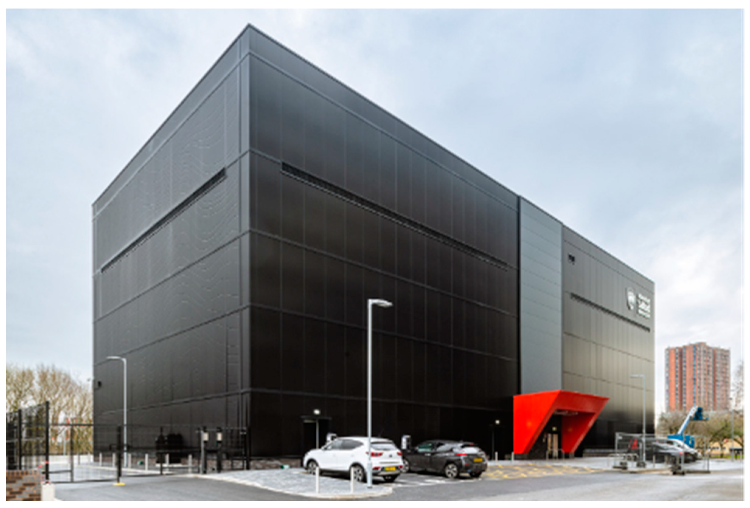
Figure 2.
eHome2 inside Environmental Chamber 1 in Energy House 2.0.
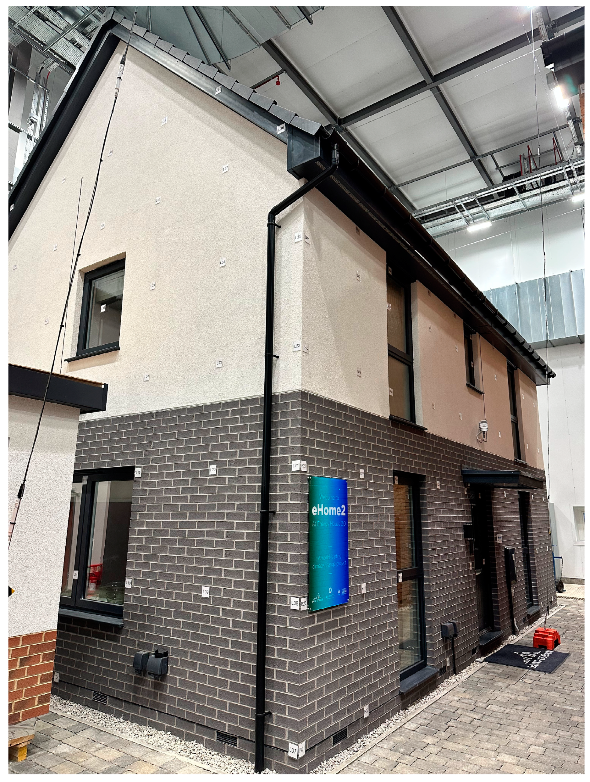
Figure 3.
Model of eHome2 in DesignBuilder.
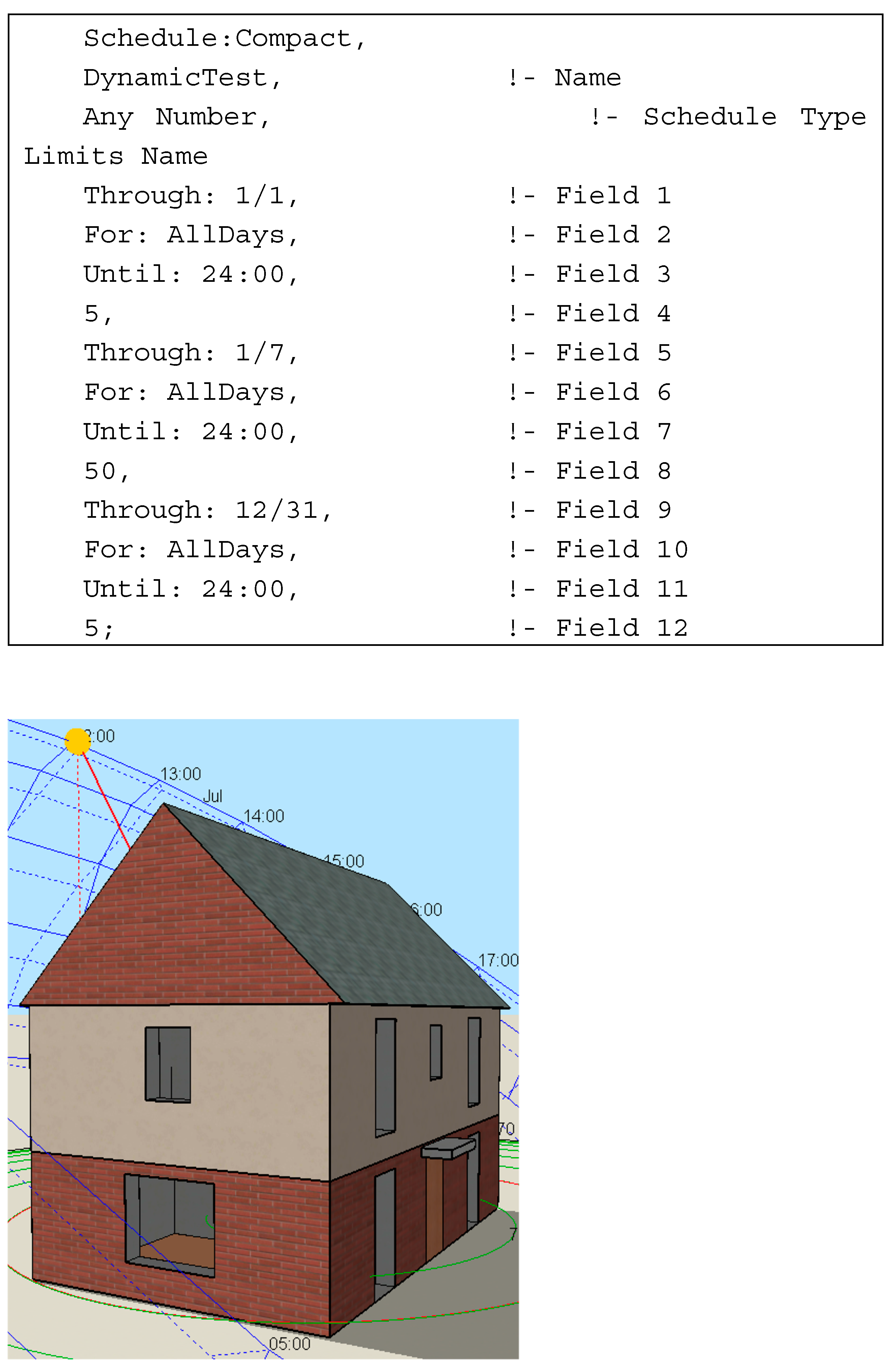
Figure 4.
Dynamic heating and cooling schedule in EnergyPlus.
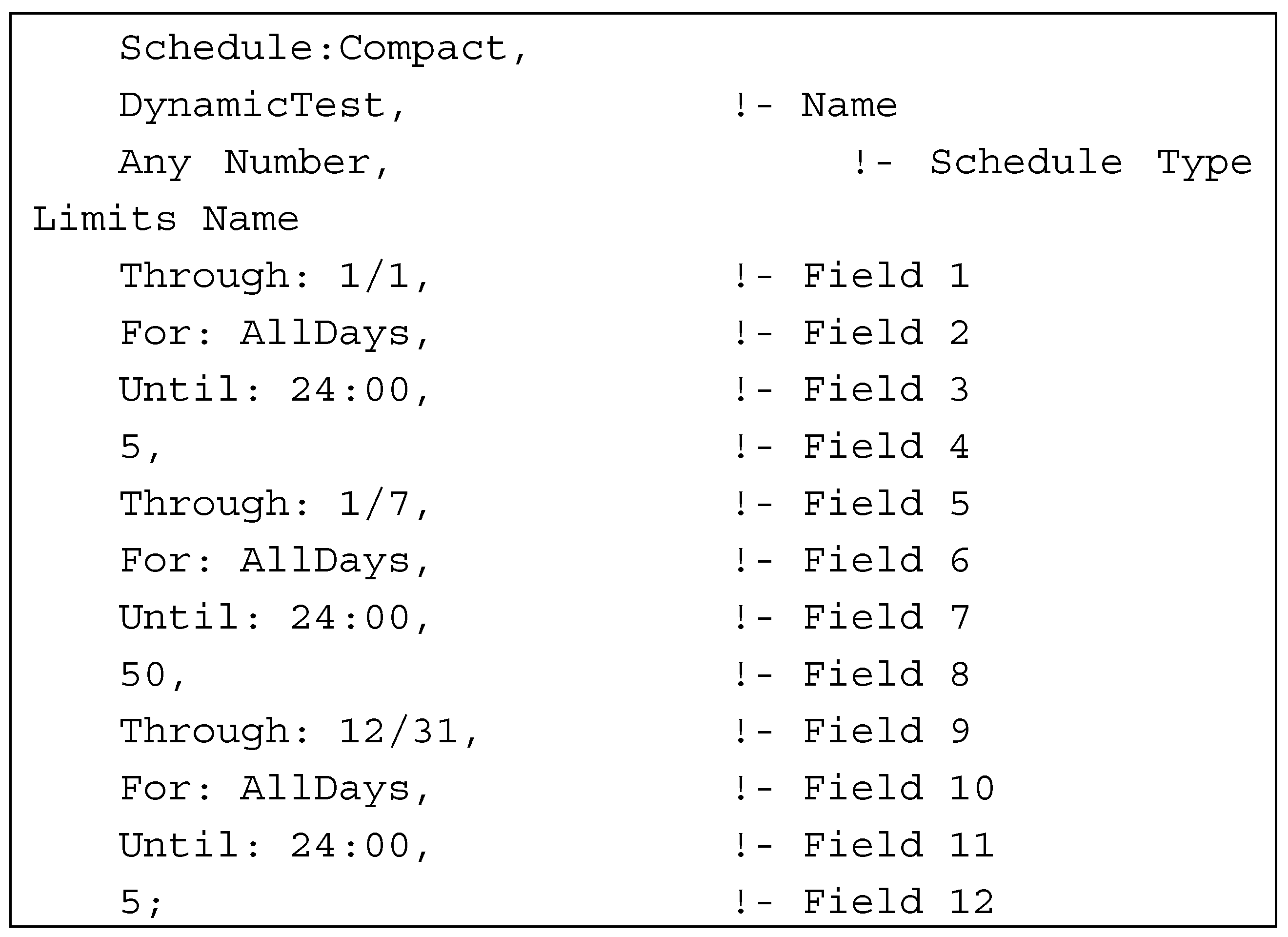
Figure 5.
Diagram of air temperature and humidity sensor locations within the chambers.
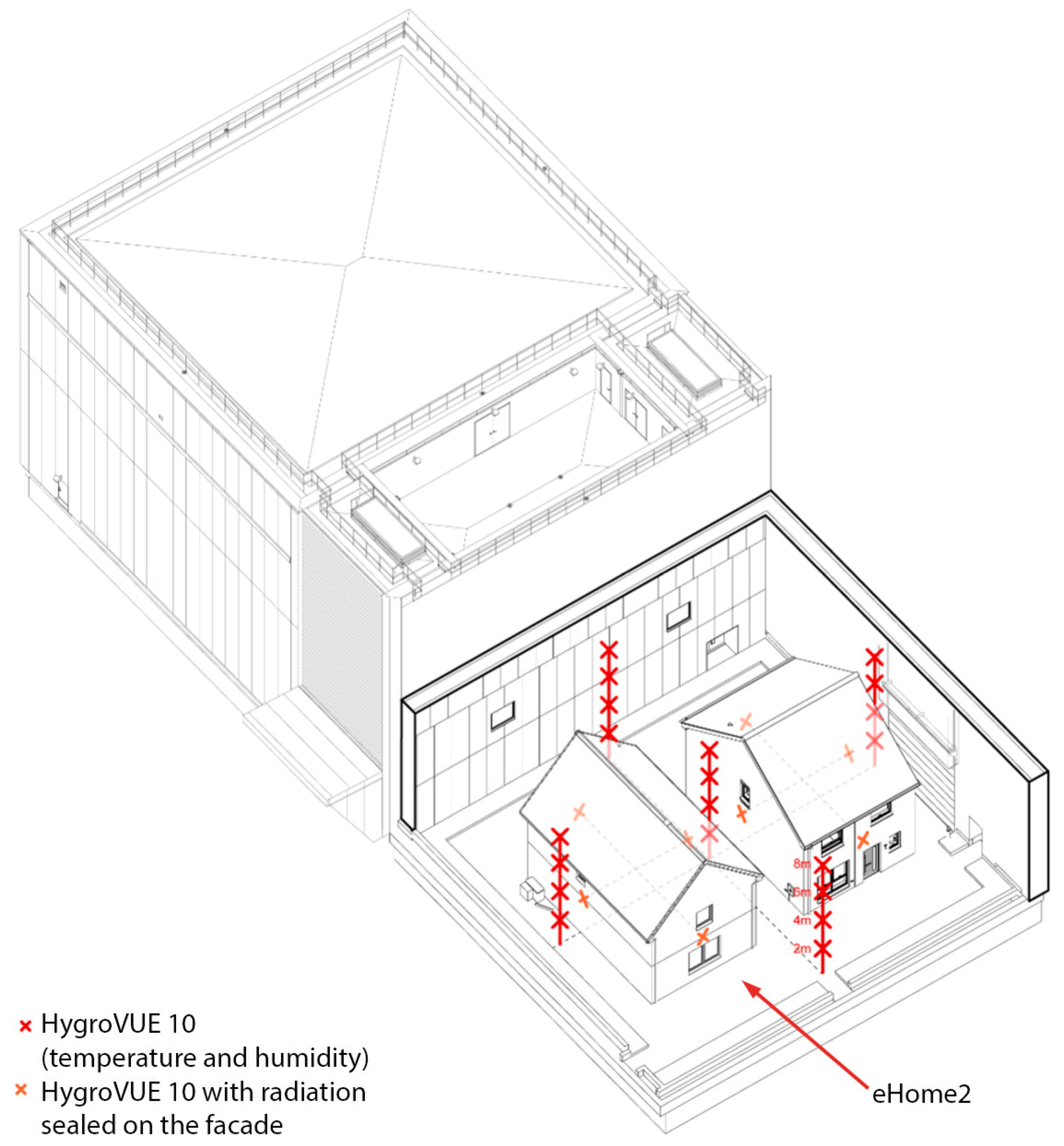
Figure 6.
Heating emitters and thermocouples in eHome2 downstairs (left) and upstairs (right).
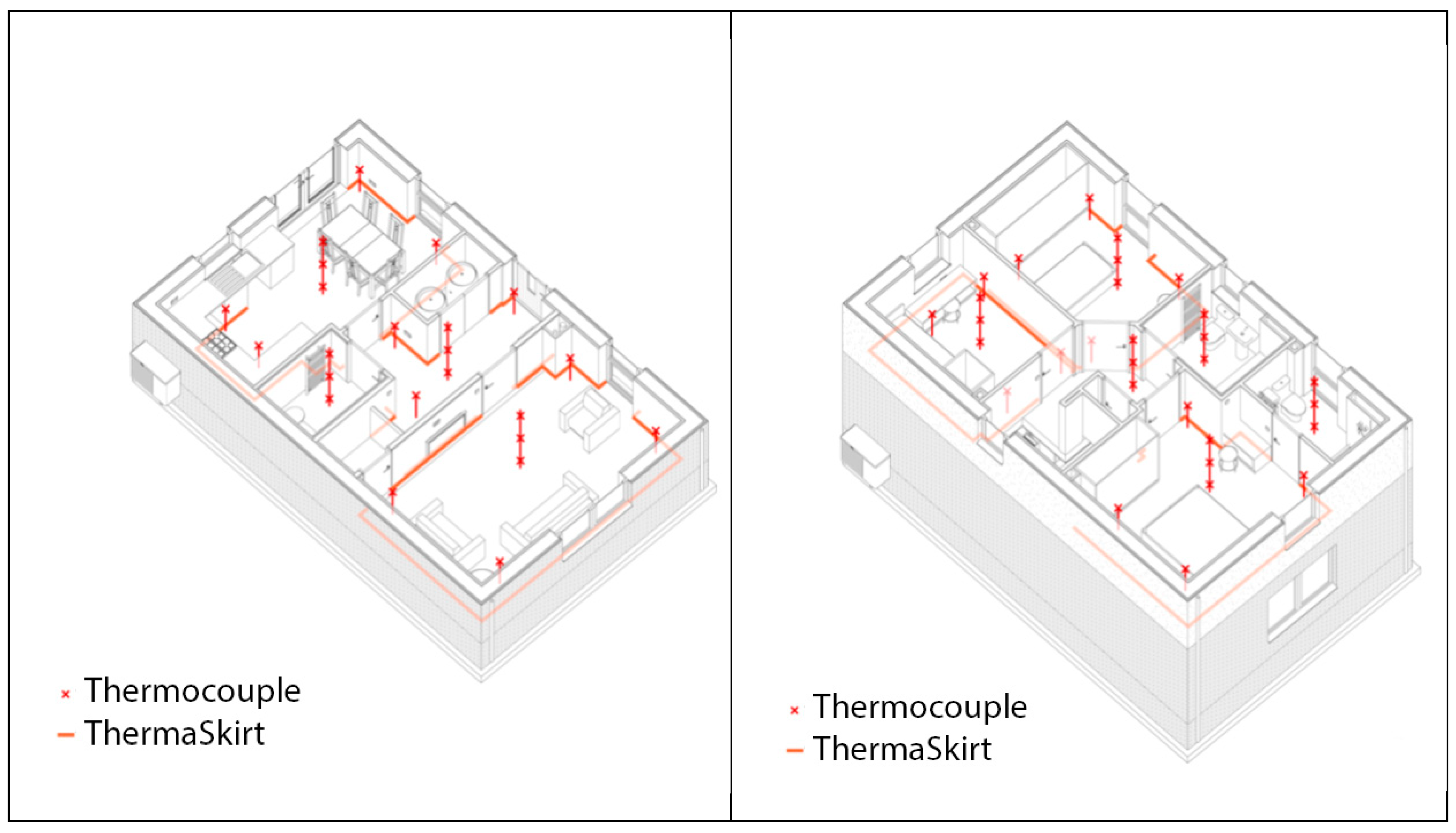
Figure 7.
Results of the dynamic heating and cooling simulation.
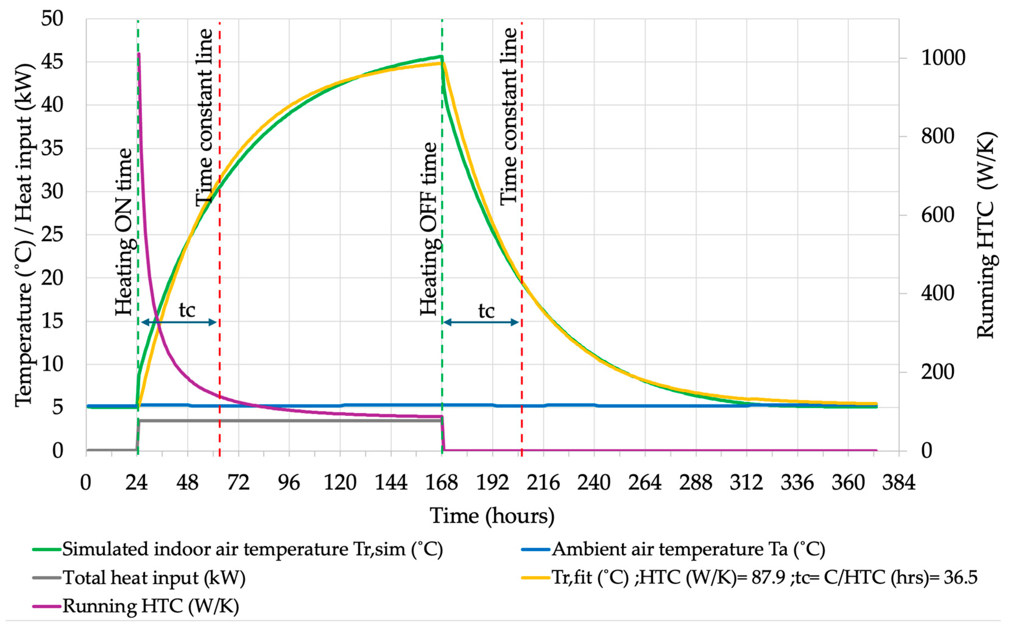
Figure 8.
HTC obtained through machine learning from measured data over a period of 140 days in 2024.
Figure 8.
HTC obtained through machine learning from measured data over a period of 140 days in 2024.
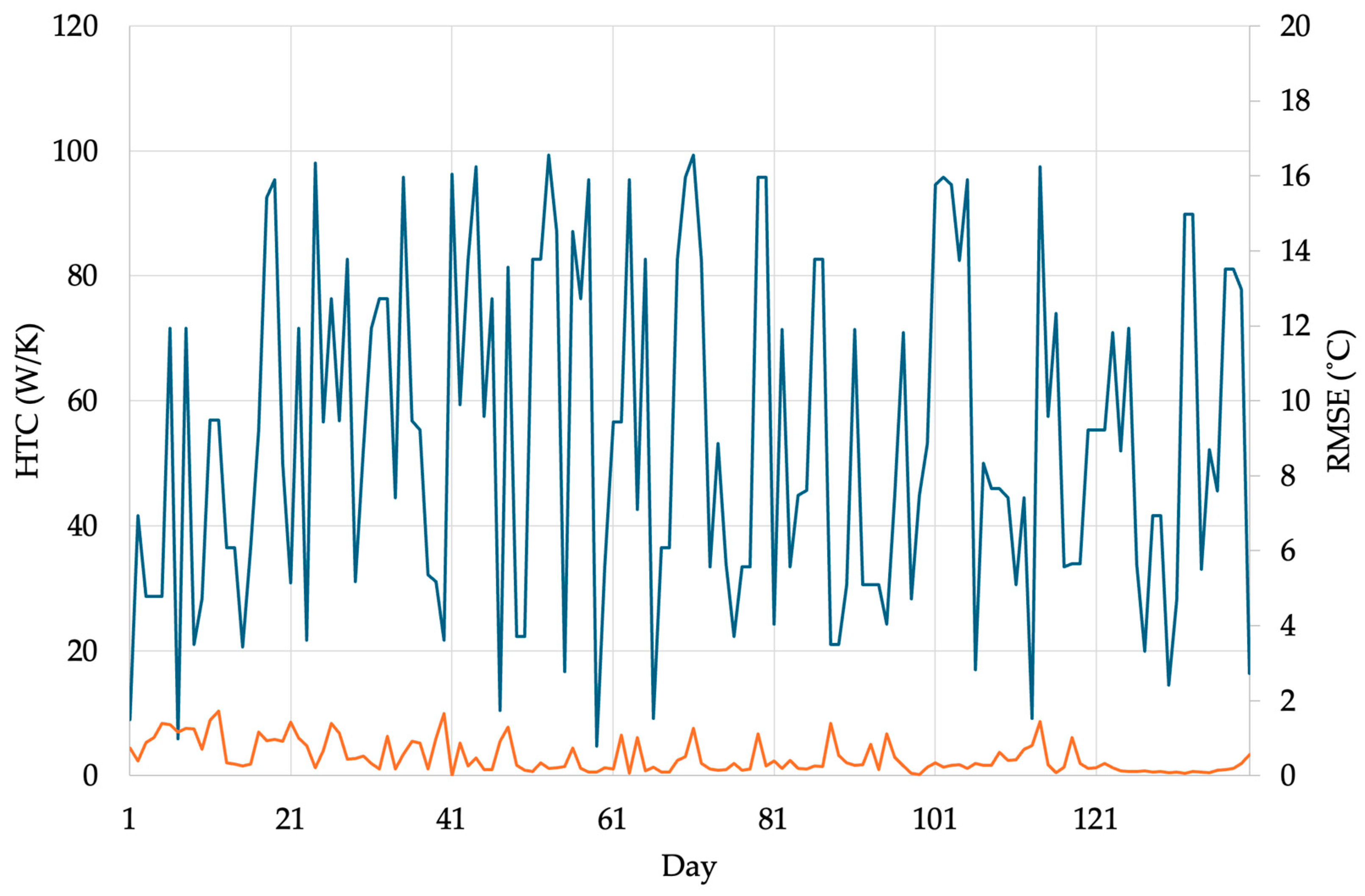
Figure 9.
HTC obtained through machine learning from measured data over a period of 12 days in 2023.
Figure 9.
HTC obtained through machine learning from measured data over a period of 12 days in 2023.
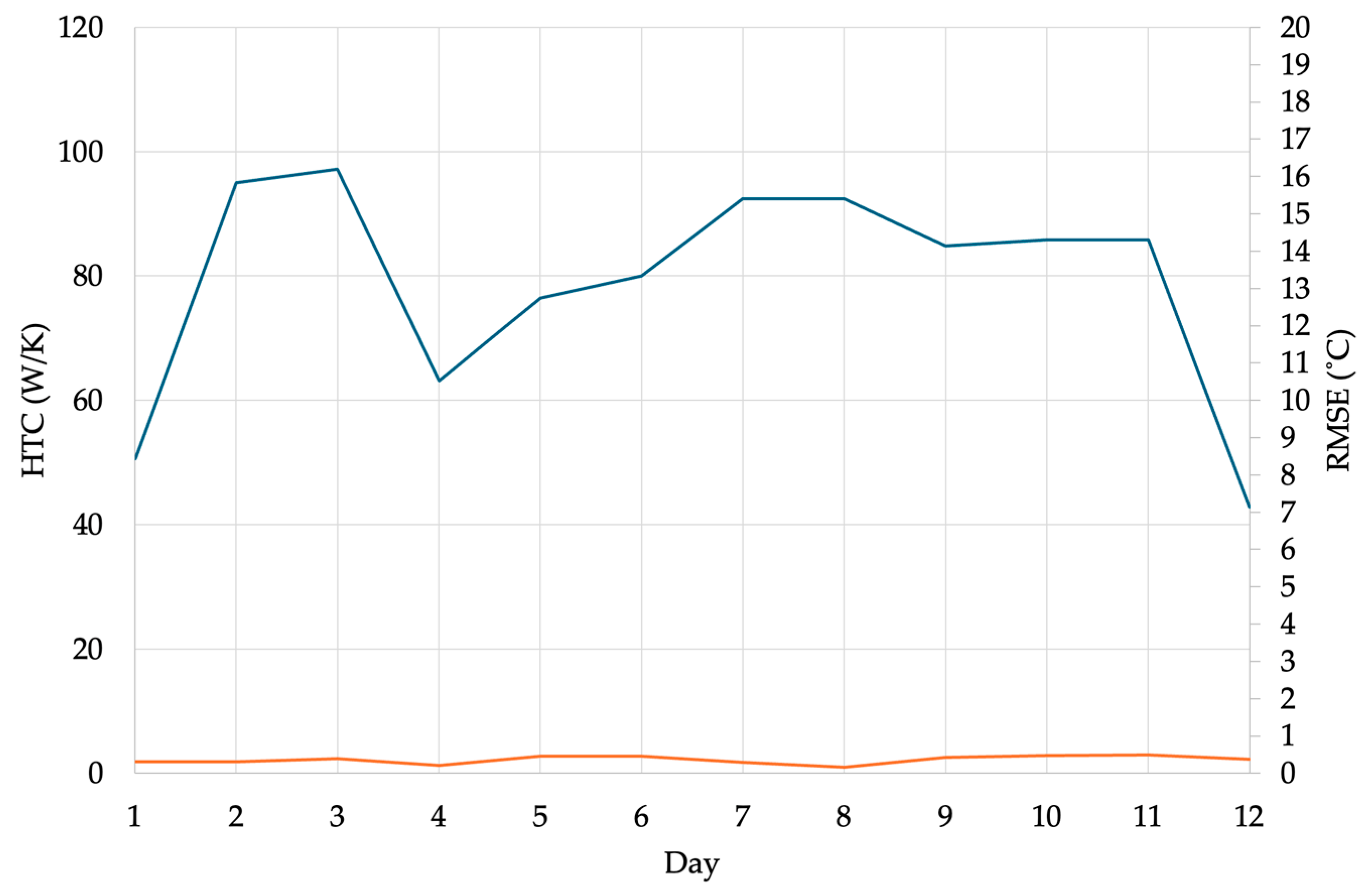

Table 1.
HTC measured using three different methods (Source: [21]).
Table 1.
HTC measured using three different methods (Source: [21]).
| HTC measurement method |
HTC value (W/K) |
Difference from coheating (%) |
| Coheating | 76.7±2.1 | |
| QUB | 65.1±5.6 | -15 |
| Veritherm | 71.9 | -6 |
Table 2.
eHome2 constructions (adapted from [27]).
Table 2.
eHome2 constructions (adapted from [27]).
| Layer | Material | Thickness (mm) | Conductivity (W/mK) |
Thermal resistance (m2K/W) |
| Brick external wall | ||||
| External finish | Weberwall brick slip finishing system | 15 | 0.72 | 0.021 |
| External board | BG glassroc x | 12.5 | 0.1865 | 0.067 |
| Cavity | Ventilated cavity | 25 | - | 0.71 |
| Sheathing | Oriented Strand Board | 9 | 0.13 | 0.069 |
| Outer Insulation | TFR35 Insulation, 8.8% bridging with flange (λ = 0.13) | 47 | 0.035 | 0.947 |
| Core insulation | TFR35 Insulation, 1.7% bridging with flange (λ = 0.13) | 151 | 0.035 | 3.831 |
| Inner insulation | TFR35 Insulation, 8.8% bridging with flange (λ = 0.13) | 47 | 0.035 | 0.947 |
| Additional sheathing | Oriented Strand Board | 9 | 0.13 | 0.069 |
| Service void | Service void with 8.8% bridging with wooden battens (λ = 0.13) | 35 | - | 0.518 |
| Internal Finish | Gyproc Wallboard | 15 | 0.19 | 0.079 |
| Rendered external wall | ||||
| External finish | Webersill TF finish coat and Weberend LCA rapid base coat | 7.5 | 0.72 | 0.0104 |
| External board | BG glassroc x | 12.5 | 0.1865 | 0.067 |
| Cavity | Ventilated cavity | 25 | - | 0.71 |
| Sheathing | Oriented Strand Board | 9 | 0.13 | 0.069 |
| Outer Insulation | TFR35 Insulation, 8.8% bridging with flange (λ = 0.13) | 47 | 0.035 | 0.947 |
| Core insulation | TFR35 Insulation, 1.7% bridging with flange (λ = 0.13) | 151 | 0.035 | 3.831 |
| Inner insulation | TFR35 Insulation, 8.8% bridging with flange (λ = 0.13) | 47 | 0.035 | 0.947 |
| Additional sheathing | Oriented Strand Board | 9 | 0.13 | 0.069 |
| Service void | Service void with 8.8% bridging with wooden battens (λ = 0.13) | 35 | - | 0.518 |
| Internal Finish | Gyproc Wallboard | 15 | 0.19 | 0.079 |
| Loft ceiling | ||||
| Primary insulation | Isover Spacesaver roof insulation | 300 | 0.044 | 6.818 |
| Secondary insulation | Isover Spacesaver roof insulation, 9% bridging with wooden batons (λ = 0.13) | 100 | 0.044 | 2.092 |
| Ceiling | Gyproc Wallboard | 15 | 0.19 | 0.079 |
| Pitched roof construction | ||||
| External | Concrete tiles (roofing) | 10 | 1.5 | 0.007 |
| Ventilation | Air gap | 10 | - | 0.15 |
| Underlayment | Roofing Felt | 5 | 0.19 | 0.026 |
| Internal partitions | ||||
| Surface 1 | Gypsum plasterboard | 15 | 0.19 | 0.079 |
| Air space | Air gap | 100 | - | 0.15 |
| Surface 2 | Gypsum plasterboard | 15 | 0.19 | 0.079 |
| Internal floor construction | ||||
| Floor surface | Caberdek chipboard floor | 22 | 0.13 | 0.169 |
| Sheathing | Oriented Strand Board | 15 | 0.13 | 0.115 |
| Air space | Air gap 254 mm | 254 | - | 0.230 |
| Ceiling | Gyproc wallboard | 15 | 0.19 | 0.079 |
| Ground floor construction | ||||
| Floor construction | 450 mm NUG375+75 mm Screed | 450 | 0.058 | 7.759 |
| External door construction | ||||
| Door | Painted Oak | 35 | 0.19 | 0.184 |
Table 3.
Calculated U-values of eHome2 (Source [27]).
Table 3.
Calculated U-values of eHome2 (Source [27]).
| Building component | U-Value (W/m2K) |
| Brick external wall U-value | 0.13 |
| Rendered external wall U-value | 0.13 |
| Loft ceiling U-value | 0.11 |
| Ground floor U-value | 0.11 |
| Windows U-value | 1.20 |
| French Door U-value | / |
| External Door U-value | 1.20 |
| Internal partition U-value | 1.89 |
| Internal floor U-value (W/m2K) | 1.16 |
| Internal door U-value (W/m2K) | 2.82 |
Table 4.
Measurement equipment used in eHome2 heating system tests.
| Measurement | Equipment | Uncertainty |
| ASHP energy and power output | Sharkey 775 heat meter | ± 1% |
| ASHP flow rate | Sharkey 775 ultrasonic flow meter | ± 1% |
| ASHP flow and return temperature | PT-100 RTD | ± 0.3 °C |
| Internal shielded air temperature | Type-T thermocouples (calibrated to ± 0.1 °C) | ± 0.1 °C |
| Mid-room shielded air temperatures | Campbell Scientific HygroVUE10(20 to 60 °C)2 | ±0.1 °C |
| Chamber air temperatures | Campbell Scientific HygroVUE10(–40 to 70 °C)2 | ±0.2 °C |
| Element surface temperatures | Type-T thermocouples (calibrated to ± 0.1 °C) | ± 0.1 °C |
| Relative humidity | Campbell Scientific HygroVUE10 | ± 1.5% |
| Black globe temperature | Type-T thermocouple in 40 mm diameter globe | ± 0.1 °C |
Table 5.
eHome2 floor areas (Source [27]).
Table 5.
eHome2 floor areas (Source [27]).
| Individual zone index i | Zone | Floor area (m2) | |
| Ground Floor | 1 | Living Room | 17.17 |
| 2 | Hall | 7.81 | |
| 3 | Kitchen + Dining | 7.77+6.35 | |
| 4 | WC | 2.79 | |
| - | Store 1 | 1.68 | |
| First Floor | 5 | Bedroom 1 | 12.29 |
| 6 | Bedroom 2 | 9.86 | |
| 7 | Bedroom 3 | 7.51 | |
| 8 | Landing | 6.09 | |
| 9 | Bathroom | 3.89 | |
| 10 | En-suite | 3.19 | |
| - | Store 2 | 0.44 |
Disclaimer/Publisher’s Note: The statements, opinions and data contained in all publications are solely those of the individual author(s) and contributor(s) and not of MDPI and/or the editor(s). MDPI and/or the editor(s) disclaim responsibility for any injury to people or property resulting from any ideas, methods, instructions or products referred to in the content. |
© 2025 by the authors. Licensee MDPI, Basel, Switzerland. This article is an open access article distributed under the terms and conditions of the Creative Commons Attribution (CC BY) license (http://creativecommons.org/licenses/by/4.0/).
Copyright: This open access article is published under a Creative Commons CC BY 4.0 license, which permit the free download, distribution, and reuse, provided that the author and preprint are cited in any reuse.


