
Submitted:
20 March 2025
Posted:
21 March 2025
You are already at the latest version
Abstract
This work proposes a hybrid deep learning-based framework to visual feedback control an eye-in-hand robotic system. The framework uses an early fusion approach in which real and synthetic images define the training data. The first layer of a ResNet-18 backbone is augmented to fuse interest-point maps with RGB channels, enabling the network to capture scene geometry better. A manipulator robot with an eye-in-hand configuration provides a reference image, while subsequent poses and images are generated synthetically, removing the need for extensive real data collection. The experimental results reveal that this enriched input representation significantly improves convergence accuracy and velocity smoothness compared to a baseline that processes real images alone. Specifically, including feature point maps allows the network to discriminate crucial elements in the scene, resulting in more precise velocity commands and stable end-effector trajectories. Thus, integrating additional, synthetically generated map data into convolutional architectures can enhance the robustness and performance of the visual servoing system, particularly when real-world data gathering is challenging.
Keywords:
visual servoing
; deep learning
; early fusion
; robot vision
1. Introduction
Visual servoing [1,2] is an advanced control technique that uses visual feedback to dynamically guide and adjust robot movements in real time. This technique utilizes data from cameras and visual sensors to provide feedback on the robot’s environment and object interaction, enabling precise and adaptive control. [3,4]. Numerous studies and advances in visual servoing have been conducted so far in domains such as end-effector pose control of a manipulator [5,6], grasping [7,8,9,10,11], robot navigation [12,13] or in medical applications [14,15,16]. The visual sensor can be positioned either on the robot itself, known as the "eye-in-hand" configuration, or elsewhere in the workspace, known as the "eye-to-hand" configuration. This paper will focus on examining the eye-in-hand configuration.
Visual servoing can be generally classified into two main types: Image-Based Visual Servoing (IBVS) and Position-Based Visual Servoing (PBVS). The first architecture, IBVS, operates directly in the image space using visual features extracted from camera images to control robot motion [17]. The primary advantage of IBVS is its robustness to camera calibration errors and environmental changes, as it does not rely on precise 3D models. Instead, IBVS adjusts the robot’s position based on real-time feedback from image features, making it suitable for dynamic and unpredictable environments. However, IBVS’s challenges are its sensitivity to local minima and the complexity of handling large displacements, which can lead to instability and inaccuracies. In contrast, PBVS uses the geometric relationship between the camera and the target object to calculate the robot’s pose in 3D space. [18] This method relies on an accurate camera calibration and a precise model of the environment to compute control commands. PBVS provides a global view of the task, allowing for more predictable and stable control than IBVS. However, its dependence on accurate models and calibration makes it less robust to environmental changes and errors in model estimation.
Recent advancements in deep learning have demonstrated significant potential for improving visual feedback control [8,9,10,11,19]. Unlike traditional methods that rely on manually crafted features, deep learning techniques enable systems to learn and extract features automatically from raw visual input. Convolutional Neural Networks (CNNs) have proven particularly effective when working with images because they can autonomously learn pertinent features specific to a given problem without predefined feature extraction techniques. For example, [19] presents a training procedure for a CNN to aproximate the unknown inverse dynamics of the robot’s inner-loop, allowing feedforward compensation to correct tracking error. The network is trained on data gathered from iterative learning control and then refined by transfer learning with real robot data to handle model discrepancies and improve performance.
To facilitate rapid training, numerous neural architectures have been developed based on CNNs pre-trained for classification tasks, such as AlexNet [20], VGG-16 [21], and FlowNet [22]. In [8], Saxena et al. used FlowNet to conduct visual servoing tasks across different environments without requiring prior knowledge of camera parameters or scene geometry. Their approach involved predicting the camera’s pose by entering concatenated images representing the current and the final desired scenes. Bateux et al. [9] presented neural architectures derived from AlexNet and VGG-16, designed to predict transformations in a camera using two images. These architectures were tailored for high-precision, robust, real-time six-degrees-of-freedom (DOF) positioning tasks utilizing visual feedback. They employed a synthetic training dataset to enhance learning efficacy and improve robustness against changes in lighting conditions. [10] introduced DEFINet, a Siamese neural architecture designed to extract features using two CNNs that share parameters. These features are then fed into a regression block to estimate the relative pose between the current and target images captured by an eye-to-hand camera. Ribeiro et al. [11] compared three CNN-based architectures for grasp detection, where the neural network provides a 3D pose using two input images depicting the initial and final scene layouts. The first architecture employs a single branch, where the images are concatenated along the depth dimension to form the input array, and a single regression block generates all six outputs. The second model uses the same input array but has two separate output branches for position and orientation. Conversely, the third CNN uses separate feature extractors for each input image, concatenates the extracted features, and then uses a single regression block. Experimental results indicated that the first model, which utilizes a single branch, delivered the best performance. A different approach is proposed in [23], where the authors propose a novel Mean Similarity Image Measurement Loss function that incorporates image similarity characterized by brightness, contrast, structural differences, and the L1 loss function. The methodology uses a convolutional neural network (CNN) based on the ResNet-152 architecture to predict 6-degree-of-freedom (DOF) pose information from monocular images. The training data is generated using a spherical projection data generator, which ensures uniform data distribution and efficient collection. Experimental results demonstrate that the proposed method achieves higher pose prediction accuracy and robustness against occlusion than traditional methods.
This work aims to design and evaluate a hybrid deep learning framework for visual servoing tasks. The proposed approach incorporates additional valuable information into the input layers and leverages transfer learning from a CNN pre-trained for image classification. The chosen architecture employs an early fusion approach, enabling the integration of supplementary data derived from traditional visual servoing methods. In particular, the supplementary data that extends the network’s input arrays is a set of point features.
The research introduces a visual servoing system (VS) designed to process visual feedback, which is fully trained and tested on a real dataset. The system operates without requiring any 3D model or camera parameter information. Given a desired image, the network predicts the most appropriate velocity commands for the camera. The main contributions of this work are:
- design of a VS framework utilizing an early fusion CNN-based method that employs feature points to access low-level pixel information. This design comprehensively describes the initial and final scenes for all neural inputs.
- construction of a large dataset for end-to-end VS control using a Universal Robot manipulator (UR5) and implementation of the network in a real robot as an extension of [24]
- implementation of the Deep Learning-based Visual Servoing control law in a real system using a UR5 robot
2. Hybrid Deep Learning Visual Servoing
To enable visual feedback control, camera-based visual information is used to determine the desired motion of a 6-DOF robot. The proposed approach incorporates features commonly suggested by traditional visual servoing methods and reconfigures them for direct integration into the neural network’s input layers. A key step in this process is converting the visual data into two-dimensional feature maps that match the size of the original RGB images. By leveraging these feature maps, differences between the initial and final scenes are highlighted, thereby guiding the CNN’s feature extractor to focus on regions most likely to yield valuable high-level features on the real-time visual servoing system.
2.1. Feature Points Maps
In previous work [24], three approaches to compute additional visual features were proposed, classified by offering different levels of details:
- feature points can be considered as low-level information, as they pinpoint exact regions in the image where one or more objects of interest appear
- segmented regions can be considered as mid-level information, offering a broader understanding of an object’s location and attributes by partitioning the image into distinct areas
- image moments can be considered high-level information by summarizing the distribution of pixel intensities within an image. This summary can estimate the object’s pose and separate linear from angular camera velocities.
The experimental results from [24] indicated that the best results were obtained with feature points and segmented regions. Therefore, for the real-time implementation, feature points are considered as additional information for the early fusion-based architecture.
Enhancing the input data to the convolutional neural network involves incorporating information derived from interest point operators. These operators are designed to identify key locations in an image while maintaining robustness to scale, rotation, and image quality variations. The resulting interest points, typically obtained from camera images, can compute the discrepancy between the robot’s current and desired positions relative to a target object or feature.
Previous studies have utilized various point detectors to extract distinctive image characteristics and estimate robotic motion. For instance, in [25], the authors present a visual servoing strategy based on SIFT feature points to track a moving object. This method employs a camera mounted on an anthropomorphic manipulator to preserve a specified relative pose between the camera and the objects of interest. Their findings demonstrate that SIFT features, invariant to scale and rotation, can reliably track an object along a trajectory. The remaining stable feature points enable the recovery of the camera’s motion through epipolar geometry, ultimately determining the robot’s joint angles via inverse kinematics. Another interesting technique is presented in [26], where the authors introduce an object-tracking technique utilizing SURF local feature points. Their visual servo controller extracts geometric features from the detected interest points, ensuring robustness against occlusion and changes in viewpoint. The effectiveness of this approach was validated using a robotic arm equipped with a monocular eye-in-hand camera operating in a cluttered environment.
The proposed approach examines the effect of early fusion on the performance of the SURF (Speed-Up Robust Features) [27] operator. SURF was selected for its demonstrated efficiency, robustness against noise, and rapid computation. Spatial information about object locations within the scene can be learned by employing a map of detected SURF points. SURF achieves this by approximating the Hessian matrix using integral images, facilitating fast and reliable feature detection. Incorporating these interest point variations from the initial to the final frame can provide additional context for a CNN, ultimately enhancing its ability to discern differences between frames and improving its overall performance.
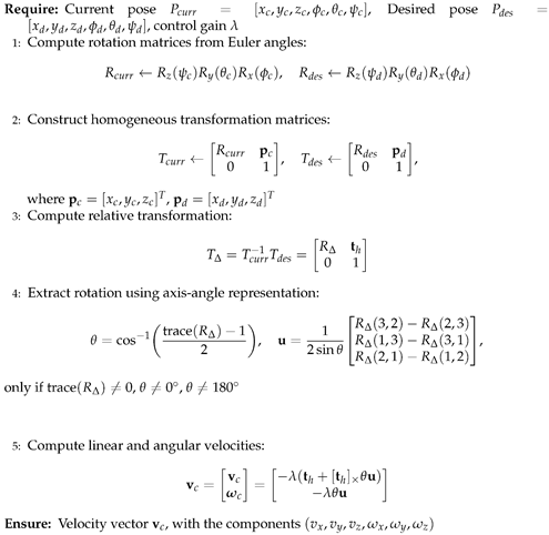
Algorithm 1 details the procedure for generating additional maps, where detected feature points are represented with higher grayscale values than the surrounding pixels. The process begins by converting the input RGB images to grayscale and applying a pre-existing SURF feature detection algorithm. The identified points are then transferred into a two-dimensional map that aligns with the early fusion template proposed in this work. Their neighborhoods are defined using a Gaussian filter with a size and a standard deviation of size . Finally, the resulting map is produced by combining the neighborhoods surrounding all the feature points. Figure 1 provides an example of SURF detections in a scene containing multiple objects. Here, the maps were generated with approximately 10% of the smallest dimension of the original images and . This augmented information helps guide the CNN to more effectively discern differences between the initial and final configurations, ultimately enhancing the accuracy of the regression task.
| Algorithm 1:Generation of Feature Point Maps Using SURF |
Require: An RGB image I (e.g., or )
|
2.2. CNN-Based Visual Servoing Control
Traditional approaches to visual feedback control often rely on precisely crafted features or geometric computations. In contrast, the proposed framework adopts an early fusion strategy that integrates SURF feature point maps with RGB images, overcoming the focus on standard visual inputs. This methodology enhances the contextual information available to the neural network, improving the robustness and accuracy for specific visual servoing applications. The key element of the proposed approach involves integrating additional contextual data directly with RGB data. By performing this integration early on, the model learns how visual information correlates with control commands, leading to a more unified and precise control mechanism.
The proposed network architecture is illustrated in Figure 2, where the input tensors are constructed by concatenating the following arrays along the depth dimension:
- , an RGB image representing the initial scene configuration.
- , an RGB image representing the desired scene configuration.
- and , each of size , which are additional feature maps derived from and , respectively. These maps provide supplementary information that can enhance the learning process.
Given that the additional information are feature points maps, the resulting array will be of size , because the concatenation is performed on depth. Therefore, each pixel in the final array will incorporate RGB values and the derived feature points. This direct concatenation allows a neural network to access visual and interest-point information simultaneously without needing separate input channels. This early fusion method also ensures against possible inaccuracies in detecting feature points since the original images and are retained in the input, allowing the CNN to glean essential information directly.
The expanded input tensors, which have a greater depth to accommodate the extra maps, then pass through a feature extraction module composed of convolutional and pooling layers. This module’s primary role is to generate a condensed representation of the input, facilitating the subsequent computation of linear and angular velocities. While the details of the feature extraction and fully connected layers can vary, they should be tailored to the input and output dimensions of the network. A common practice is to adopt a CNN trained initially for image classification, such as ResNet [28], and adapt its architecture for regression tasks. In this work, ResNet-18 is modified by adjusting its final layers to handle regression outputs and, depending on the type of additional maps, the first convolutional layer is revised to account for the increased number of input channels.
An advantage of the proposed framework lies in its promise for real-time functionality. The modifications introduced by the proposed framework do not substantially increase the complexity of the deep model but instead focus on altering the input arrays. The SURF-incorporated maps require two auxiliary maps to depict the initial and final scenes, each having dimensions and pixel intensities ranging from 0 to 255.
A further modification arises in the first convolutional layer since pre-trained networks assume RGB inputs and possess filters of size , where F is the filter dimension. These filters expand to in the proposed framework. While the original weights can be used as an initialization, it is essential to account for the relevance of the newly incorporated maps. Specifically, the channels associated with and can inherit . In contrast, the remaining two channels (whether segmentation or feature-point maps) are initialized through a grayscale conversion of the pre-trained RGB weights
where represents the updated filter obtained by merging the red (), green (), and blue () channels of . These parameters are further fine-tuned during training to align with the regression objective.
All layers from the pre-trained model can be retained within the fully connected block except for the final layer, which should consist of six neurons—one for each camera velocity to be estimated. Additionally, the activation function in the last layer must permit both positive and negative outputs, thus excluding certain nonlinearities such as ReLU. By way of illustration, ResNet-18 layers are incorporated into the architecture shown in Figure 2, which results in an SURF feature maps-based early fusion architecture.
3. Dataset Configuration
For the actual system to effectively perform the visual servoing task, it is essential to construct a dataset that accurately reflects the environmental characteristics in which the robot will operate. This dataset must address the task’s requirements and demonstrate enough variability to ensure strong generalization. The data collection scenario employs a UR5 collaborative robot fitted with an “eye-in-hand” setup based on a ZED Mini stereo camera. Figure 3 presents the real-time application setup used for this work.
Figure 4 shows how this robotic system’s physical and computational layers are unified through ROS (Robot Operating System). The physical layer comprises a ZED Mini camera and a UR5 robot observed in Figure 3, linked by motion dependency so that any robot movement directly affects the captured visual data. The camera acquires images and sends them through USB to the camera node in the computational layer. At the same time, the robot concurrently transmits its pose data to the robot node via Ethernet.
Within the ROS-based computation layer, the application node operates as the primary central unit, utilizing GPU acceleration to handle image and pose data efficiently. Using this information, it calculates velocity commands and relays them to the robot node, thereby directing the UR5 robot’s real-time movements. This integrated design ensures precise data acquisition and processing, forming the backbone for robust visual servoing and broader generalization.
To create the dataset, a strategy inspired by [9] was adopted, in which an entire dataset is synthetically generated from a single reference RGB image and its corresponding pose. Figure 5 presents the reference pose used in this work which was acquired with the camera at the pose (m, m, m, rad, rad, rad).
One effective strategy for generating additional camera views around a known reference pose is introducing slight perturbations in translation and rotation. Specifically, the translation components and rotation components are drawn from a Gaussian distribution
where centers the distribution at the reference pose, and determines the variations of the poses. This approach naturally clusters samples around the reference due to the Gaussian peak at zero offset and maintains a smooth distribution over the six dimensions of rigid motion.
To ensure realistic camera movement, the Gaussian parameters must be carefully set. In particular, translational offsets are sampled with a standard deviation [m], while rotational offsets use for and , and for . These values keep the new poses within small but meaningful deviations from the reference. Moreover, incorporating bounds for both translation (e.g., ) and rotation guards against implausibly significant shifts while promoting diversity in the synthesized dataset.
Even though these offsets arise from a Gaussian, some poses may still be unrealistic for a specific application. One can impose bounding rules on each newly sampled pose to address this. After a perturbation is drawn, the camera’s 3D position and rotation angles are examined to ensure they remain within fixed limits, for instance radians for rotation or meters for translation. This validation step ensures that synthetic viewpoints stay within a feasible range, filtering out outliers with excessive displacement or rotation.
Once a sampled pose is obtained, it is checked against specific thresholds. For instance, allowable shifts in the x and y directions might be set to meters, with meters permitted in z. Likewise, rotational changes could be limited at relative to the original orientation. Any pose outside these bounds is discarded and resampled. This mechanism maintains a balanced spread of valid viewpoints without straying into physically unrealistic regions achieved by the UR5 robot.
When the camera encounters a minor alteration in pose while observing a planar region of the scene, the connection between the original and new images can be described by a homography [29]. In computer vision, a homography is a projective mapping that takes points from one image of a planar surface to their counterparts in another image captured under a pinhole camera model. This concept underpins key operations, such as image registration and rectification, that align images from differing viewpoints [30,31]. Formally, if and represent the homogeneous coordinates of corresponding points in the first and second images, respectively, they are related by
where ≈ indicates equality up to a scale factor, consistent with the nature of homogeneous coordinates.
Consider a plane specified by , where is the normal and d is the distance from the camera. The homography for a planar surface in 3D can be written as
where and denote the rotation and translation between the two viewpoints. Including the camera intrinsic matrix yields the final 2D projective transformation,
which fully describes how to warp the original image to approximate the new viewpoint.
The matrix encodes the camera’s internal parameters: horizontal and vertical focal lengths and the principal point . Incorporating ensures consistent projection into the image plane for both the reference and transformed poses. Since variations in focal length or principal point placement can greatly alter how transformations appear in pixel coordinates, applying and on either side of the homography is crucial for accurate image warping.
During homographic transformation, some regions in the warped output may lack corresponding pixels in the source image. To fill these missing points, a background color is estimated using a k-means clustering approach. The reference image is reshaped into a set of pixel-value vectors, and k-means is run (with a small number of clusters, selected empirically) to identify the dominant color. The cluster containing the largest number of pixels is assumed to represent the background, and its centroid is used for filling. This ensures newly exposed areas match the overall appearance of the scene.
One can generate numerous new images from a single reference by iteratively sampling random perturbations, checking them against spatial and rotational bounds, and computing the resulting homographies. Each warped image corresponds to a distinct but still constrained viewpoint in proximity to the original pose. Such synthetic datasets are highly valuable for algorithm development in fields like feature tracking, camera calibration, or visual odometry, where coverage of various positions and orientations is beneficial. Algorithm 2 summarizes the main steps explained earlier.
| Algorithm 2:Synthetic Dataset Generation |
|
An example of using Algorithm 2 is illustrated next. Starting from a reference image depicted in Figure 5, two randomly generated images are shown in Figure 6. The image on the left was synthetically generated at the pose (m, m, m, rad, rad, rad), while the image on the right was synthetically generated at the pose (m, m, m, rad, rad, rad)
As Figure 2 shows, the early fusion-based CNN architecture predicts velocities, so a conversion from poses to velocities is necessary to train the network. The velocities were computed by converting the difference between the current and desired robot poses into velocity commands. Specifically, given the initial and desired robot poses represented by Euler angles and positions, homogeneous transformation matrices are first constructed. The relative transformation between these two poses is computed, and the rotational component is extracted using axis-angle representation. Finally, a proportional control law is applied to determine linear and angular velocities, employing a control gain parameter . Algorithm 3 succinctly summarizes this process, illustrating how the velocity vector is derived directly from pose information, thus enabling efficient and precise visual servoing control.
The experimental results are detailed in the following section.
| Algorithm 3 Pose-to-Velocity Computation |
 |
4. Experimental Results
This section highlights the significance of extra input-level information in a neural architecture through an experimental analysis conducted for the previously introduced approach. Using Resnet-18 as baseline, the architecture was modified following Figure 2, with the input array defined for input images of size .
4.1. Training Setup
Using the method described in Section 3, 600 synthetic images were generated. To create all the pairs from this set, a binomial coefficient was considered, which represents the number of ways to choose k items from n options, mathematically expressed as:
For each pair , reversed order was also included, effectively doubling the final count of pairs to 359400 sampling data. This procedure results in a comprehensive sampling of relative poses between any two images in the dataset, a sampling being represented by the triplet [, , ]. These triplets were divided into three groups for training, validation, and testing. Specifically, 70%
Table 1 presents the key hyperparameters and computational settings used during training. The Adam optimizer is used with a piecewise learning rate schedule and an initial rate of . A mini-batch size 256 per GPU is employed to leverage the parallel processing capabilities of three NVIDIA A100 Tensor Core GPUs, each equipped with 40 GB of memory. To mitigate overfitting, an L2 regularization term of is applied. Training progresses for 100 epochs, and the validation process is triggered once per epoch, after every iterations, with a patience of 10 for early stopping. The loss function is defined as the root mean squared error (RMSE), which is well-suited for the regression objective of this work.
4.2. Offline Results
To evaluate the performance of the trained neural models, the mean squared output error (MSE) is adopted for testing samples. Being a recognized metric in regression tasks, the MSE measures the average squared difference between the predicted and actual velocity values. By examining the MSE across the various datasets, one can infer the model’s ability to generalize and its effectiveness in accurately estimating the target velocity vectors. The MSE over all output channels for a particular dataset is defined in (6)
where S denotes the number of samples in the dataset, is the ground truth, and represents the network’s output for the channel of the sample.
Table 2 presents the MSE computed for the testing dataset, where stands for the model which takes ResNet-18 as baseline and does not include the early fusion approach at the neural input level, while the second model stands for the model designed by the architecture proposed in Figure 2 with SURF feature points as additional data.
The experiment demonstrates that additional maps assist CNNs in concentrating on significant details. Consequently, the early fusion model achieves more precise approximations, indicating the value of the extra input data for the visual servoing task.
4.3. Online Results
Figure 7 presents the online testing scenario that was considered, with the corresponding desired configuration (left) and initial configuration (right). The desired image was acquired at the pose (m, m, m, rad, rad, rad), while the image on the right was acquired at the pose (m, m, m, rad, rad, rad).
Figure 8 and Figure 9 provide a comprehensive visualization of the real-time evolution of velocity commands during online testing of the two visual servoing strategies based on Deep Learning. In these experiments, a comparison is made between the ResNet approach without early fusion and the ResNet architecture with early fusion. For the considered scenario, was set at 0.25. The real-time result can be found online at https://www.youtube.com/watch?v=_Voi6tL2Xcs.
In Figure 8, linear and angular velocities decline gradually, showing minimal oscillations across all components. This gradual decay indicates that error compensation is happening in a more controlled manner, with fewer abrupt compensatory adjustments as the camera nears the target view. The additional SURF feature maps guide the network toward more reliable identification of scene discrepancies, allowing it to issue velocity updates that consistently reduce error. Building on this observation, one can see that each velocity component in Figure 8 peaks early on and then consistently decreases gradually without large secondary spikes. For instance, the velocity along the camera’s axis, which typically shows the most substantial influence on image rotation, stabilizes near zero faster than in the non-fusion approach. This suggests that the integrated features give the network a more direct handle on rotational misalignment, thus minimizing the likelihood of repeated corrective “twists” over time.
In contrast, Figure 9 displays more noticeable fluctuations in velocity commands. While these trends decrease over time, the oscillations suggest that the system occasionally overcorrects before readjusting its course, causing extra velocity cycles to increase and decrease. In practical terms, these fluctuations may extend convergence or create unstable movement. Consequently, the early fusion strategy, which merges raw RGB data with SURF-based feature maps, demonstrates a more direct route to alignment between current and desired images, delivering smoother control signals and a quicker approach to near-zero velocities in both linear and angular coordinates. Notably, this less stable convergence pattern implies that the network may struggle to discern minor yet critical discrepancies between the current and desired views without explicit feature map guidance. As a result, it can inadvertently apply larger corrective commands than necessary, followed by counter-corrections to compensate for these excesses. Consequently, repeated overshoots in the velocity curves suggest that the servoing loop deals with insufficient or ambiguous visual feedback, prompting corrective commands that exceed the ideal target.
Figure 10 presents the pixel-level mean squared error for the two earlier analyzed architectures. The MSE between a reference (desired) image A and each current image that is acquired from the robot, I, is defined by
where H, W, and C denote the image’s height, width, and number of color channels, respectively.
As observed, the architecture based on the early fusion approach demonstrates the lowest overall error, which most effectively minimizes the pixel-level discrepancy between the reference image and each newly acquired view during the robot’s motion. The Mean Squared Error (MSE) values of 1000 and 2000 correspond to the pixel-level squared errors between images obtained from the early fusion and non-early fusion approaches, respectively. Since MSE is expressed in squared pixel units, the average pixel error is determined by taking the square root. Therefore, an MSE of 1000 for the early fusion method translates to an average pixel error of approximately pixel intensity values per RGB channel. The non-early fusion method, with an MSE of 2000, results in a significantly higher average pixel error of approximately . Considering an image, this notable difference underscores the superiority of the early fusion approach, providing images substantially closer to the reference or desired configuration.
From the neural architecture point of view, by combining additional feature descriptors like SURF points with the raw RGB data, this architecture utilizes more comprehensive visual information, which leads to more precise image-space alignment as the robot converges to the target pose. Meanwhile, the ResNet architecture without early fusion yields the highest error, indicating that relying exclusively on RGB data for velocity prediction lacks the essential details required for accurate pixel-level alignment. Overall, these pixel-level MSE results confirm that the early fusion strategy provides superior performance in matching the current camera view to the desired reference image.
5. Conclusions
This paper presents a novel hybrid deep learning approach to visual servoing control systems. As a main contribution, the approach integrates raw RGB image data with feature point maps using an early fusion architecture. This innovative methodology offers several key advantages over traditional visual servoing techniques, paving the way for more robust and efficient robotic control in dynamic environments. The seamless integration of diverse data sources is a crucial element of this work, improving performance metrics across various aspects of the visual servoing pipeline.
A contribution of this research is the creation of a comprehensive dataset combining real-world data captured using a UR5 robotic arm in an eye-in-hand configuration and a synthetically generated dataset. This dual approach addresses the limitations of relying solely on real or synthetic data. Real-world data captures the complexities and nuances of real-world scenarios, including lighting variations, occlusions, and unforeseen disturbances. However, collecting sufficient real-world data can be time-consuming, expensive, and potentially dangerous. Synthetic data, on the other hand, allows for generating vast amounts of labeled data under controlled conditions, addressing the limitations of real-world data acquisition. Combining both datasets provides a rich and diverse training ground for the deep learning models, leading to improved generalization and robustness.
Two distinct neural network architectures based on the robust ResNet framework were designed and trained using this combined dataset. One architecture directly incorporated additional feature maps into the input layer, while the other processed the RGB and feature map data separately before fusion. A comparative analysis of these architectures demonstrated the superior performance of the early fusion approach, which combines the raw RGB images and feature point maps at the earliest stage of the network’s processing. This early fusion strategy proved particularly effective in enhancing offline prediction accuracy and the convergence speed of the online servoing process. The results indicate the benefits of integrating diverse data sources to achieve superior performance in visual servoing tasks.
Looking ahead, some promising directions exist for extending this work. First, investigating alternative real-time representations, such as optical flow or depth-based maps, may provide more accurate contextual information for the neural architecture. Another interesting aspect of future work may involve refining the network to predict not just the velocity commands but also the 3D pose of the robot or camera in space.
Author Contributions
Conceptualization, A.-P.B. and A.B.; methodology, A.-P.B. and A.B.; software, A.-P.B. and A.-I.I.; validation, all; formal analysis, A.-P.B.; investigation, A.-P.B.; resources, all; data curation, A.-P.B.; writing—original draft preparation, A.-P.B.; writing—review and editing, all; visualization, all; supervision, A.B.; project administration, A.B.; All authors have read and agreed to the published version of the manuscript.
Funding
This research is supported by the project “Romanian Hub for Artificial Intelligence - HRIA”, Smart Growth, Digitization and Financial Instruments Program, 2021-2027, MySMIS no. 334906.
Institutional Review Board Statement
Not applicable.
Data Availability Statement
The data used to support the findings of this study are available from the corresponding author upon request.
Conflicts of Interest
The authors declare no conflicts of interest.
References
- Hutchinson, S.; Hager, G.D.; Corke, P.I. A tutorial on visual servo control. IEEE transactions on robotics and automation 1996, 12, 651–670. [Google Scholar] [CrossRef]
- Chaumette, F.; Hutchinson, S. Visual servo control Part I: Basic approaches. IEEE Robotics & Automation Magazine 2006, 13, 82–90. [Google Scholar]
- Chaumette, F.; Hutchinson, S. Visual servo controlPart II: Advanced approaches. IEEE Robotics & Automation Magazine 2007, 14, 109–118. [Google Scholar]
- Chaumette, F.; Hutchinson, S.; Corke, P. Visual Servoing. In Handbook of Robotics; Springer; pp. 841–867.
- Wilson, W.J.; Hulls, C.W.; Bell, G.S. Relative end-effector control using cartesian position based visual servoing. IEEE Transactions on Robotics and Automation 1996, 12, 684–696. [Google Scholar] [CrossRef]
- Kelly, R. Robust asymptotically stable visual servoing of planar robots. IEEE Transactions on Robotics and Automation 1996, 12, 759–766. [Google Scholar] [CrossRef]
- Haviland, J.; Dayoub, F.; Corke, P. Control of the final-phase of closed-loop visual grasping using image-based visual servoing. arXiv 2020, arXiv:2001.05650. [Google Scholar]
- Saxena, A., Pandya; Kumar, G., Gaud. Exploring convolutional networks for end-to-end visual servoing. In Proceedings of the Proc. IEEE International Conference on Robotics and Automation, Singapore; 2017; pp. 3817–3823. [Google Scholar]
- Bateux, Q.; Marchand, E.; Leitner, J.; Chaumette, F.; Corke, P. Training deep neural networks for visual servoing. In Proceedings of the Proc. IEEE International Conference on Robotics and Automation, Brisbane; 2018; pp. 1–8. [Google Scholar]
- Tokuda, F.; Arai, S.; Kosuge, K. Convolutional neural network based visual servoing for eye-to-hand manipulator. IEEE Access 2021, 9, 91820–91835. [Google Scholar] [CrossRef]
- Ribeiro, E.; Mendes, R.; Grassi, V. Real-time deep learning approach to visual servo control and grasp detection for autonomous robotic manipulation. Elsevier’s Robotics and Autonomous Systems 2021, 139, 103757. [Google Scholar] [CrossRef]
- Mateus, A.; Tahri, O.; Miraldo, P. Active structure-from-motion for 3d straight lines. In Proceedings of the 2018 IEEE/RSJ International Conference on Intelligent Robots and Systems (IROS). IEEE; 2018; pp. 5819–5825. [Google Scholar]
- Bista, S.R.; Giordano, P.R.; Chaumette, F. Combining line segments and points for appearance-based indoor navigation by image based visual servoing. In Proceedings of the 2017 IEEE/RSJ International Conference on Intelligent Robots and Systems (IROS). IEEE; 2017; pp. 2960–2967. [Google Scholar]
- Azizian, M.; Khoshnam, M.; Najmaei, N.; Patel, R.V. Visual servoing in medical robotics: a survey. Part I: endoscopic and direct vision imaging–techniques and applications. The international journal of medical robotics and computer assisted surgery 2014, 10, 263–274. [Google Scholar] [CrossRef] [PubMed]
- Mathiassen, K.; Glette, K.; Elle, O.J. Visual servoing of a medical ultrasound probe for needle insertion. In Proceedings of the 2016 IEEE International Conference on Robotics and Automation (ICRA). IEEE; 2016; pp. 3426–3433. [Google Scholar]
- Zettinig, O.; Frisch, B.; Virga, S.; Esposito, M.; Rienmüller, A.; Meyer, B.; Hennersperger, C.; Ryang, Y.M.; Navab, N. 3D ultrasound registration-based visual servoing for neurosurgical navigation. International journal of computer assisted radiology and surgery 2017, 12, 1607–1619. [Google Scholar] [CrossRef] [PubMed]
- Hashimoto, K.; Kimoto, T.; Ebine, T.; Kimura, H. Manipulator control with image-based visual servo. In Proceedings of the Proceedings. 1991 IEEE International Conference on Robotics and Automation. IEEE Computer Society; 1991; pp. 2267–2268. [Google Scholar]
- Thuilot, B.; Martinet, P.; Cordesses, L.; Gallice, J. Position based visual servoing: keeping the object in the field of vision. In Proceedings of the Proceedings 2002 IEEE International Conference on Robotics and Automation (Cat. No. 02CH37292). IEEE, Vol. 2; 2002; pp. 1624–1629. [Google Scholar]
- Chen, S.; Wen, J.T. Industrial robot trajectory tracking control using multi-layer neural networks trained by iterative learning control. Robotics 2021, 10, 50. [Google Scholar] [CrossRef]
- A.Krizhevsky.; I.Sutskever.; G.E.Hinton. ImageNet Classification with Deep Convolutional Neural Networks. Advances in neural information processing systems 2012, pp. 1097–1105.
- Simonyan, K.; Zisserman, A. Very deep convolutional networks for large-scale image recognition. International Conference on Learning Representations 2015. [Google Scholar]
- Dosovitsky, A.; Fischery, P.; Ilg, E.; Hazirbas, C.; Golkov, V.; van der Smagt, P.; Cremers, D.; Brox, T. Flownet: Learning optical flow with convolutional networks. International Conference on Computer Vision 2015, 2758–2766. [Google Scholar]
- He, Y.; Gao, J.; Chen, Y. Deep learning-based pose prediction for visual servoing of robotic manipulators using image similarity. Neurocomputing 2022, 491, 343–352. [Google Scholar] [CrossRef]
- Botezatu, A.P.; Ferariu, L.E.; Burlacu, A. Enhancing Visual Feedback Control through Early Fusion Deep Learning. Entropy 2023, 25, 1378. [Google Scholar] [CrossRef] [PubMed]
- Shademan, A.; Janabi-Sharifi, F. Using scale-invariant feature points in visual servoing. In Proceedings of the Machine Vision and its Optomechatronic Applications. SPIE, 2004, Vol. 5603, pp. 63–70.
- La Anh, T.; Song, J.B. Robotic grasping based on efficient tracking and visual servoing using local feature descriptors. International Journal of Precision Engineering and Manufacturing 2012, 13, 387–393. [Google Scholar] [CrossRef]
- Bay, H.; Ess, A.; Tuytelaars, T.; Gool, L.V. SURF: Speeded Up Robust Features. In Proceedings of the Computer Vision and Image Understanding Journal, 2008.
- He, K.; Zhang, X.; Ren, S.; Sun, J. Deep residual learning for image recognition. In Proceedings of the Proceedings of the IEEE conference on computer vision and pattern recognition, 2016, pp. 770–778.
- Dubrofsky, E. Homography estimation. Diplomová práce. Vancouver: Univerzita Britské Kolumbie 2009, 5. [Google Scholar]
- Agarwal, A.; Jawahar, C.; Narayanan, P. A survey of planar homography estimation techniques. Centre for Visual Information Technology, Tech. Rep. IIIT/TR/2005/12 2005. [Google Scholar]
- DeTone, D.; Malisiewicz, T.; Rabinovich, A. Deep image homography estimation. arXiv 2016, arXiv:1606.03798. [Google Scholar]
Figure 1.
Example of original images (left) and their corresponding points of interest maps (right).
Figure 1.
Example of original images (left) and their corresponding points of interest maps (right).
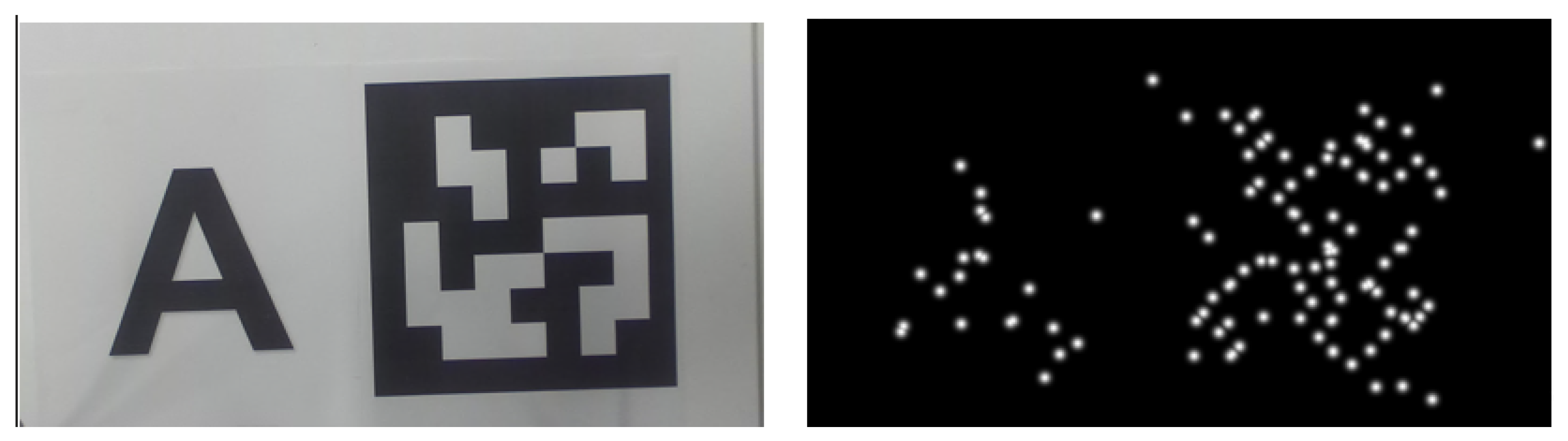
Figure 2.
Hybrid deep learning framework.
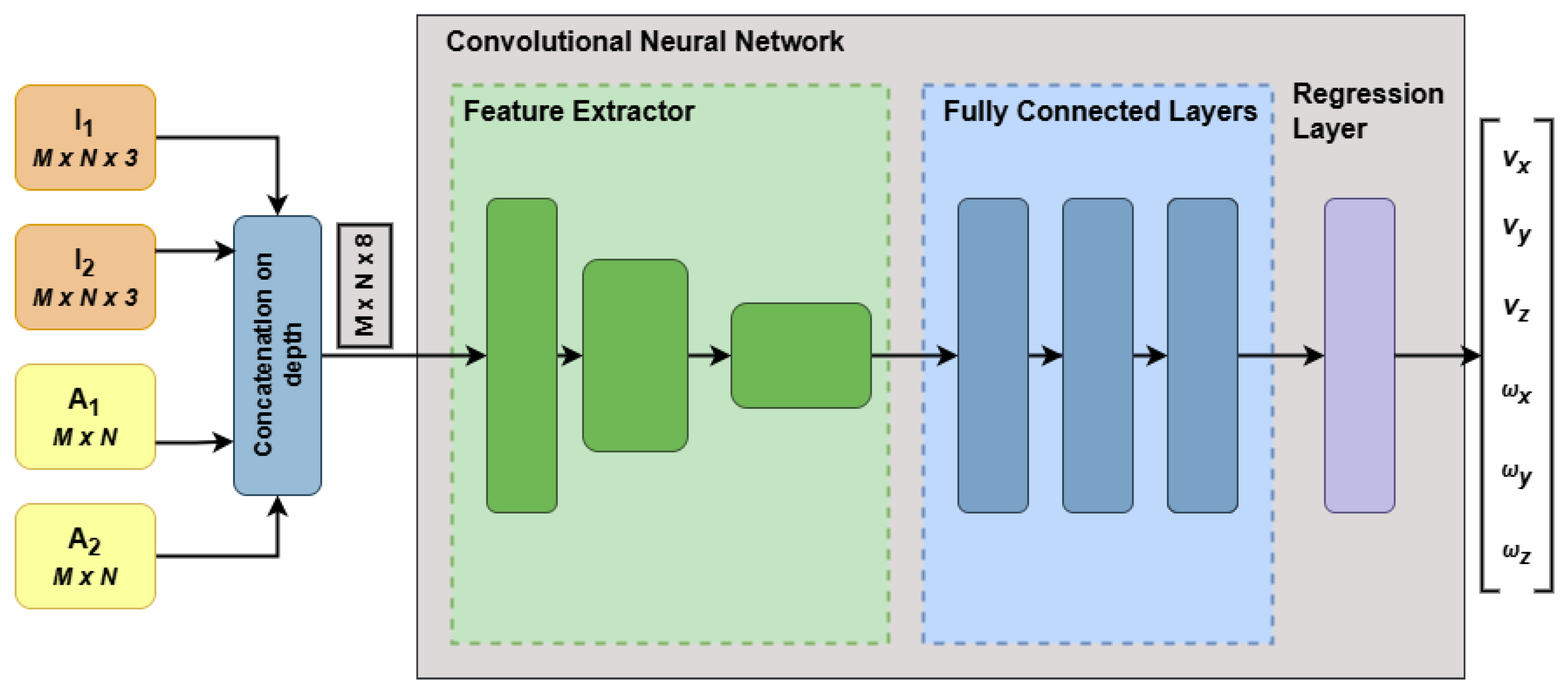
Figure 3.
Real-time application setup.
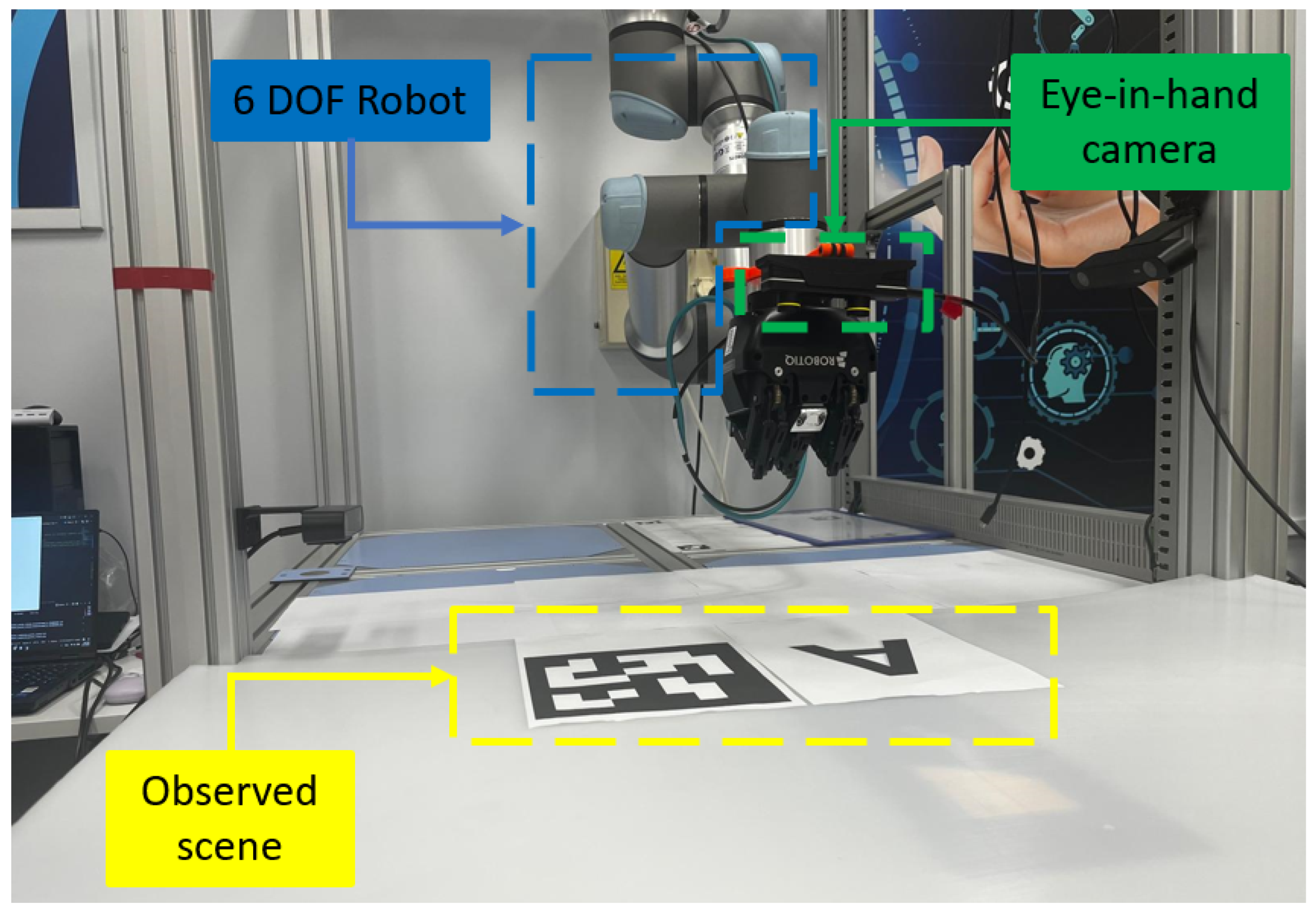
Figure 4.
System Architecture for Visual Servoing Using ROS.
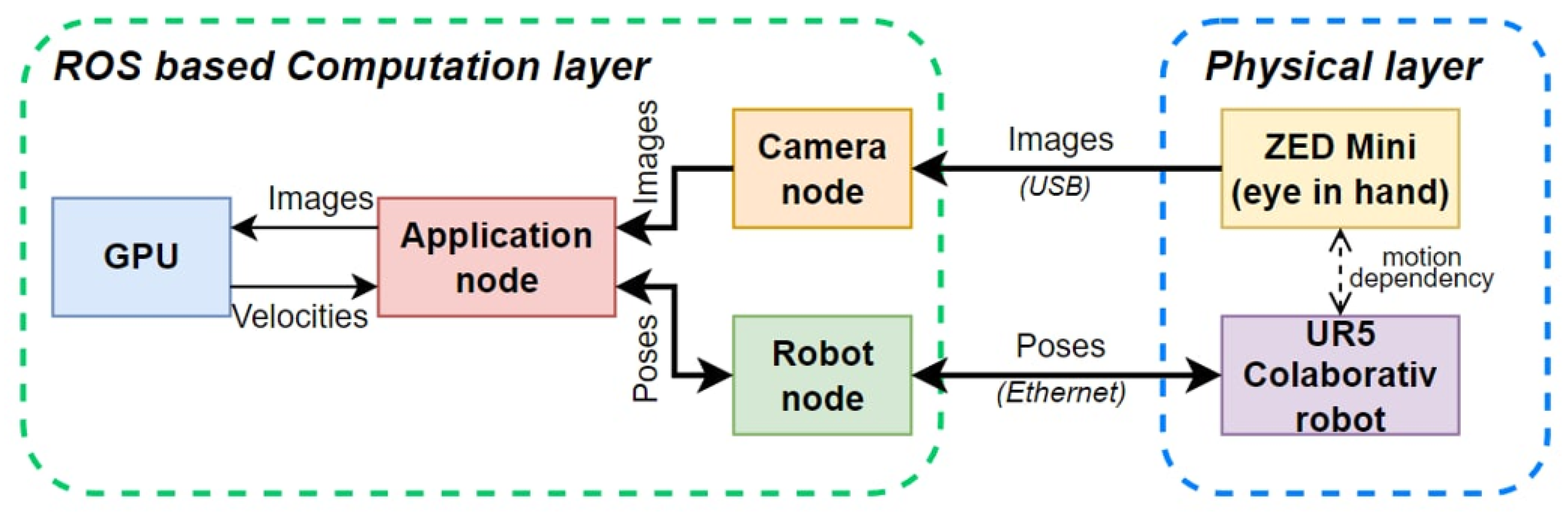
Figure 5.
Example of reference image used for synthetic generation.
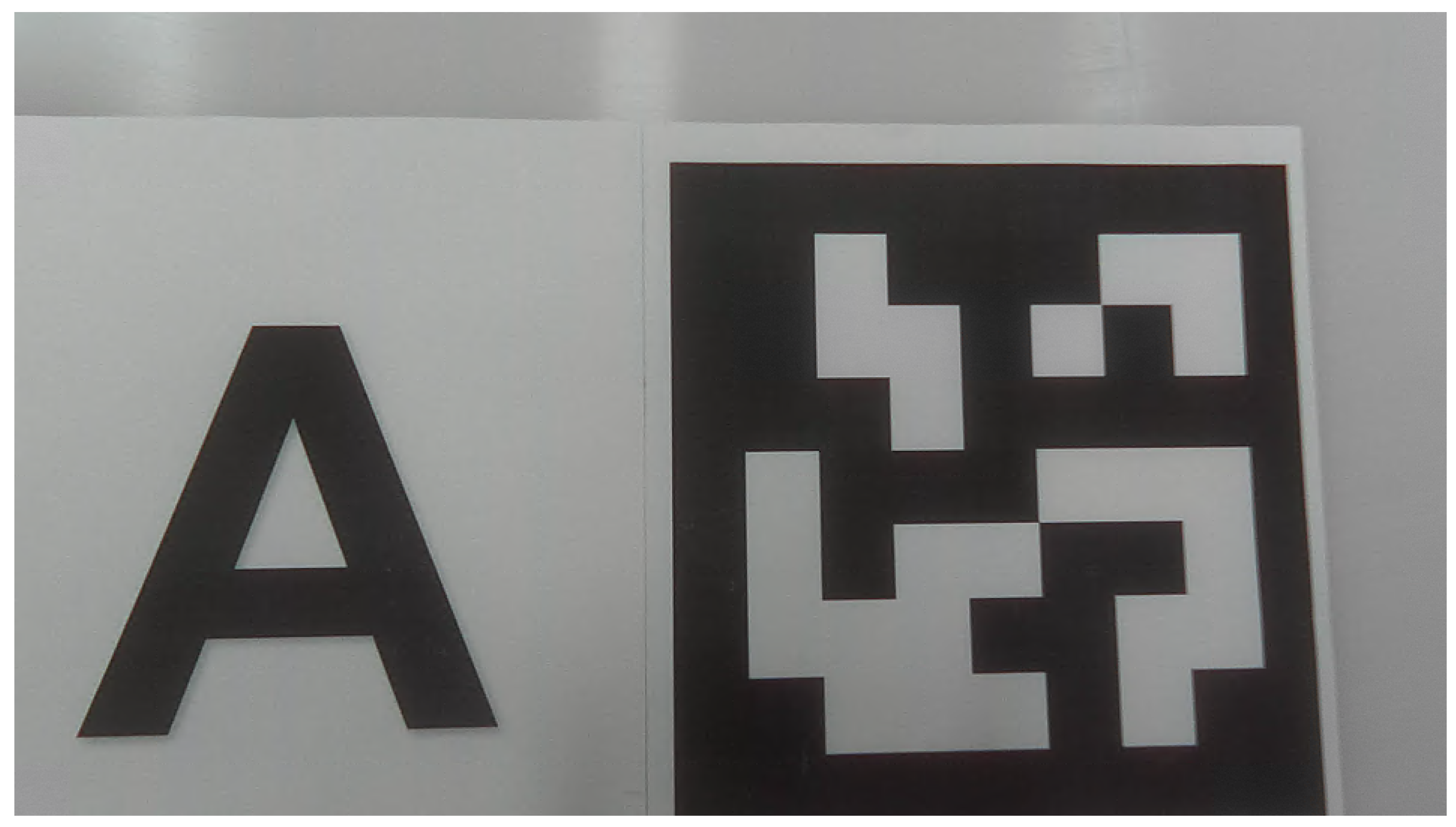
Figure 6.
Illustration of synthetic viewpoint generation using homography-based warping.
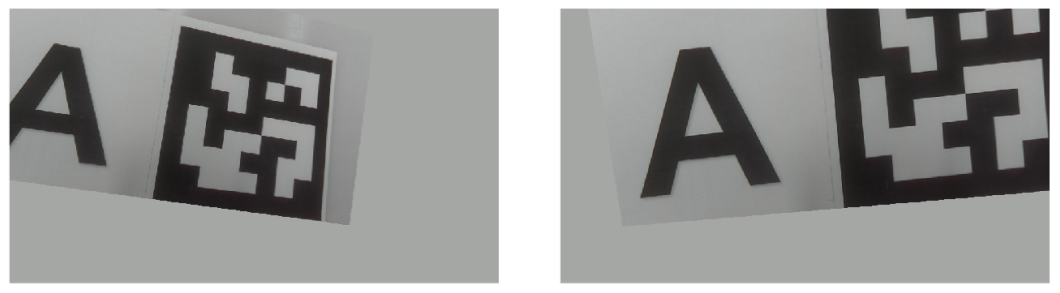
Figure 7.
An online testing scenario considered for the VS task.
Figure 8.
Velocities analysis for ResNet with early fusion.
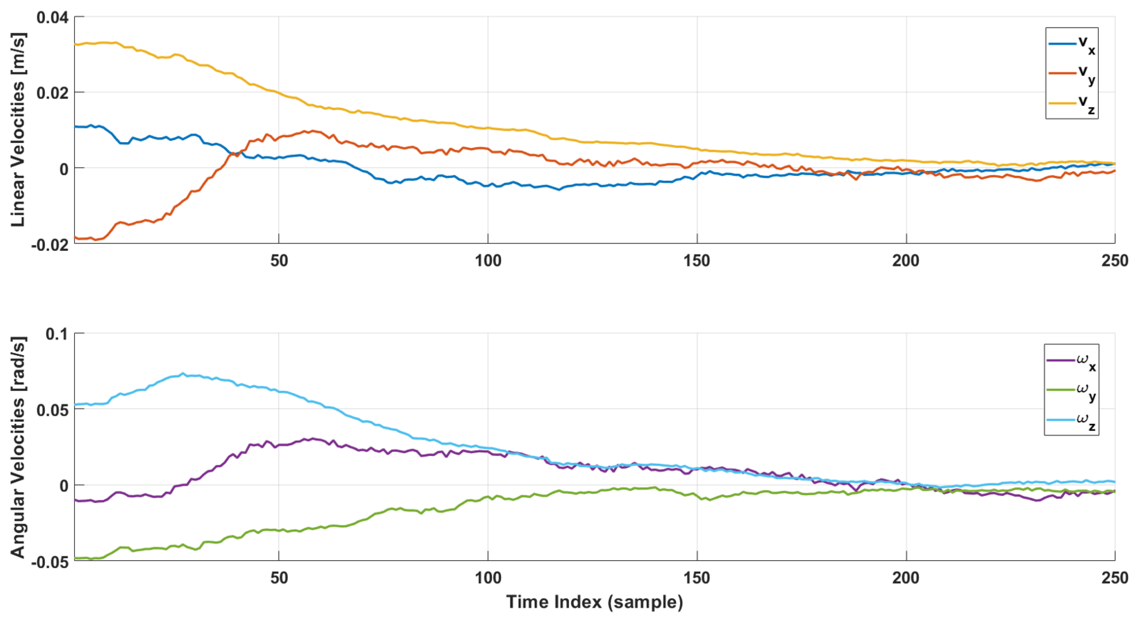
Figure 9.
Velocities analysis for ResNet without early fusion.
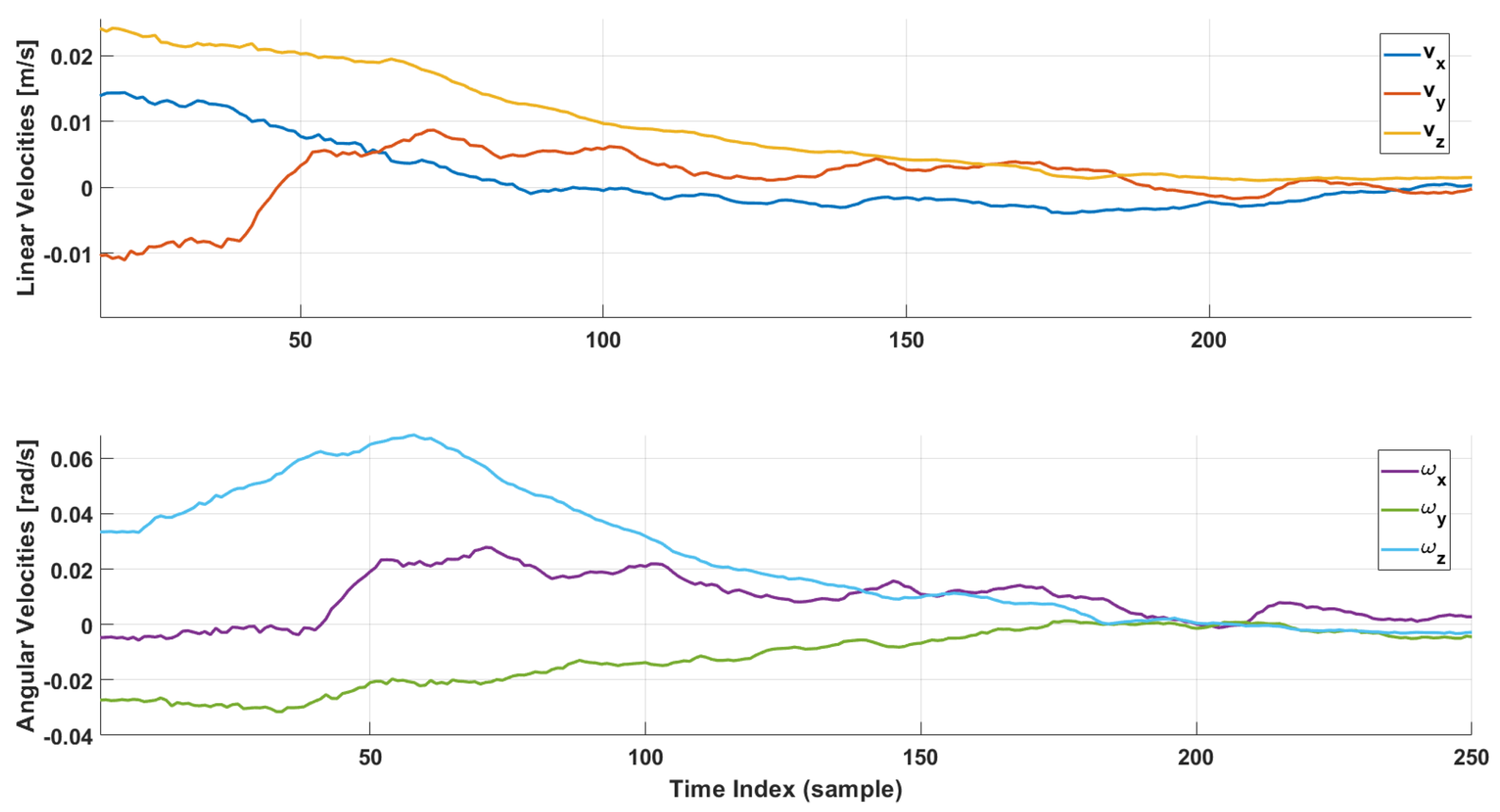
Figure 10.
Early fusion vs non-early fusion MSE comparison.
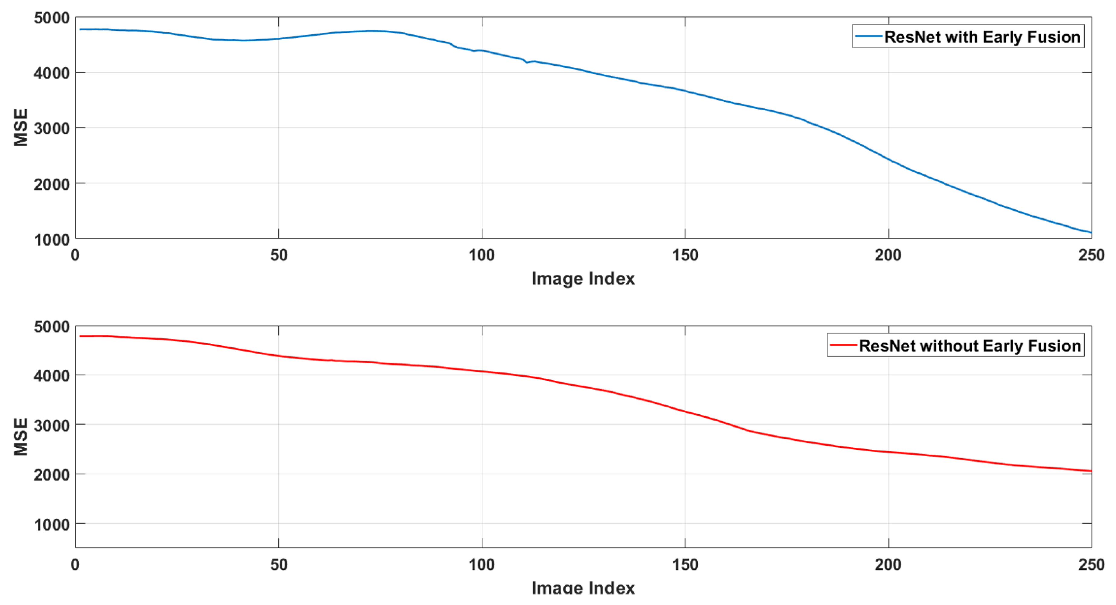

Table 1.
Summary of Training Parameters.
| Parameter | Value and Information |
|---|---|
| Training optimizer | Adam |
| Mini-Batch Size | 256 ×number of GPUs |
| GPU Setup | 3 x NVIDIA A100 Tensor Core GPU with 40 GB |
| Number of Epochs | 100 |
| Initial Learning Rate | |
| L2 Regularization | |
| Learning Rate Schedule | Piecewise |
| Learning Rate Drop Factor | 0.1 |
| Learning Rate Drop Period | 30 |
| Validation Frequency | |
| Validation Patience | 10 |
| Loss function | Root Mean Squared Error |
Table 2.
MSE for Offline testing dataset ().
| CNN | [m/s ] | [m/s ] | [m/s ] | [rad/s ] | [rad/s ] | [rad/s ] |
|---|---|---|---|---|---|---|
| Testing | ||||||
Disclaimer/Publisher’s Note: The statements, opinions and data contained in all publications are solely those of the individual author(s) and contributor(s) and not of MDPI and/or the editor(s). MDPI and/or the editor(s) disclaim responsibility for any injury to people or property resulting from any ideas, methods, instructions or products referred to in the content. |
© 2025 by the authors. Licensee MDPI, Basel, Switzerland. This article is an open access article distributed under the terms and conditions of the Creative Commons Attribution (CC BY) license (http://creativecommons.org/licenses/by/4.0/).
Copyright: This open access article is published under a Creative Commons CC BY 4.0 license, which permit the free download, distribution, and reuse, provided that the author and preprint are cited in any reuse.


