Submitted:
20 March 2025
Posted:
20 March 2025
You are already at the latest version
Abstract
We present a model of an evolving spherically symmetric dissipative self-gravitating fluid distribution which tends asymptotically to a ghost star, meaning that the end state of such a system corresponds to a static fluid distribution with vanishing total mass, and energy-density distribution which is negative in some regions of the fluid. The model is inspired in a solution representing a fluid evolving quasi-homologously and with vanishing complexity factor. However in order to satisfy the asymptotic behavior mentioned above, the starting solution has to be modified, as a consequence of which the resulting model only satisfies the two previously mentioned conditions, asymptotically. Additionally a condition on the variation of the infinitesimal proper radial distance between two neighboring points per unit of proper time is imposed, which implies the presence of a cavity surrounding the center. Putting together all these conditions we are able to obtain an analytical model depicting the emergence of a ghost star. Some potential observational consequences of this phenomenon are briefly discussed at the last section.
Keywords:
relativistic fluids
; interior solutions
; spherically symmetric sources
1. Introduction
In a recent paper [1] the concept of ghost star was introduced and studied in detail. Such a concept, inspired in early ideas by Zeldovich [2,3], describes fluid distributions which do not produce gravitational field outside its boundary surface (i.e. its total mass vanishes). In order to achieve the vanishing of the total mass (for a non-trivial fluid distribution) one must assume the existence of some regions within the fluid sphere endowed with negative energy-density. Some examples of this kind of fluid distribution may be found in [1,4,5] (see also [6] for more recent developments).
More recently we have studied solutions which, either correspond to the adiabatic evolution of a ghost star, or describe the evolution of fluid distributions which attain the ghost star status momentarily at some point of their lives, abandoning such state immediately afterward [7].
However neither of the models exhibited in the references above describe solutions leading asymptotically (as ) to a ghost star.
It is the purpose of this work to present a model of an evolving fluid distribution describing the emergence of a ghost star, as the end point of its evolution.
In order to obtain our model we have initially started by imposing three conditions
- Quasi-homologous evolution (QH)[10]
- The variation of the infinitesimal proper radial distance between two neighboring points per unit of proper time vanishes [11].
The first two conditions have been shown to be useful in the description of the structure and evolution of self–gravitating fluids. The second one represents a generalization of the well known homologous evolution in Newtonian hydrodynamics [12,13,14].
The third condition implies the existence of a cavity surrounding the center, and therefore appears to be a useful tool for the modeling of cosmic voids [15,16].
Notwithstanding, we have resorted to the above conditions for purely heuristic reasons, its physical interest being, in the context of this work, a fact of secondary relevance.
The solution obtained under the three conditions above (hereafter referred to as “primeval solution”) does not satisfy the asymptotic conditions required to obtain a static ghost star as the end point of the evolution. Accordingly we have modified this solution in order to satisfy the conditions ensuring the formation of a ghost star.
The final solution matches smoothly on the external boundary surface with the Minkowski space-time as . Instead, matching conditions are not satisfied on the boundary surface delimiting the fluid distribution from the inside (not even asymptotically), accordingly we have a thin shell on that surface.
The physical properties of the model will be analyzed in detail and the characteristics of the ghost star appearing at the end of the evolution will be discussed.
2. The General Setup of the Problem: Notation, Variables and Equations
We consider a spherically symmetric distribution of fluid, which is bounded from the outside by a spherical surface and, since we shall assume a cavity surrounding the center, the fluid is also bounded from inside by a spherical surface . The matter content consists in a locally anisotropic fluid (principal stresses unequal) undergoing dissipation in the form of heat flow (diffusion approximation).
Thus, in comoving coordinates, the general line element may be written as
where the functions depend on t and r.
The energy–momentum tensor takes the form
where is the energy density, the radial pressure, the tangential pressure, the heat flux, the four velocity of the fluid, and a unit four vector along the radial direction. These quantities satisfy
It will be convenient to express the energy momentum tensor (2) in the equivalent (canonical) form
with
Since we are considering comoving observers, we have
It is worth noticing that we do not add explicitly bulk or shear viscosity to the system because they can be trivially absorbed into the radial and tangential pressures, and , of the collapsing fluid (in ). Also we do not explicitly introduce dissipation in the free streaming approximation since it can be absorbed in and q.
2.1. Einstein Equations
Einstein’s field equations for the interior spacetime (1) are given by
2.2. Kinematical Variables and the Mass Function
The three non-vanishing kinematical variables are the four–acceleration , the expansion scalar and the shear tensor . The corresponding expressions follow at once from their definitions.
Thus
producing
with .
The expansion is given by
and for the shear tensor we have
with only one non–vanishing independent component.
2.3. The Mass Function
To study the dynamical properties of the system, let us introduce, following Misner and Sharp the proper time derivative given by
and the proper radial derivative ,
2.4. The Junction Conditions
Outside we have the Vaidya spacetime (or Schwarzschild in the dissipationless case), described by
where denotes the total mass, and v is the retarded time. The matching of the non-adiabatic sphere to the Vaidya spacetime, on the surface constant, in the absence of thin shells (Darmois conditions [19], see also [20]), implies the continuity of the first and the second fundamental forms through the matching hypersurface, producing
and
In the case when a cavity forms we also have to match the solution to the Minkowski spacetime on the boundary surface delimiting the empty cavity (). In this case the matching conditions imply
As we shall see below, in our model the Darmois conditions cannot be satisfied on , in which case we must allow the presence of thin shells on , implying discontinuities in the mass function [21].
On the other hand Darmois conditions are satisfied on but only asymptotically (as ). In other words a thin shell is present on during the evolution, disappearing as the ghost star forms.
2.5. The Transport Equation
In the diffusion approximation we shall need a transport equation to evaluate the temperature and its evolution within the fluid distribution. Here we shall resort to a transport equation derived from a causal dissipative theory ( e.g. the Israel-Stewart second order phenomenological theory for dissipative fluids [22,23,24]).
Thus the corresponding transport equation for the heat flux reads
where denotes the thermal conductivity, and T and denote temperature and relaxation time respectively. Observe that, due to the symmetry of the problem, equation (30) only has one independent component, which may be written as
In the case we recover the Eckart–Landau equation [25,26], and in the Newtonian limit we recover the Cattaneo equation [27,28,29]
3. Three Conditions Leading to Our Model
As mentioned before we shall start the building up of our model by imposing three conditions on the fluid distribution, these are: the vanishing complexity factor condition, the quasi–homologous condition and a kinematical condition on the variation of the infinitesimal proper radial distance between two neighboring points per unit of proper time. In what follows we shall briefly describe these conditions.
3.1. The Vanishing Complexity Factor Condition
The complexity factor is a scalar function that has been proposed in order to measure the degree of complexity of a given fluid distribution [8,9].
The complexity factor is identified with the scalar function which defines the trace–free part of the electric Riemann tensor (see [9] for details).
It can be expressed in terms of physical variables as
or in terms of the metric functions
We shall impose the vanishing of the complexity factor in order to find an analytical solution, however as we shall see below, such a solution does not satisfy the required asymptotic behavior. In order to obtain a model with the appropriate asymptotic behavior we shall modify this primeval solution, as a consequence of which the resulting model will satisfy the vanishing complexity factor condition only asymptotically.
3.2. The Quasi-Homologous Condition
The QH condition is a generalization of the homologous condition (H) which has been assumed in [9] to represent the simplest mode of evolution of the fluid distribution. However this last condition appears to be too stringent thereby excluding many potential interesting scenarios. Therefore in [10] we have proposed to relax (H), and replaced it by what we called the “quasi–homologous” condition (QH).
More specifically, the H condition implies that
and
where and denote the areal radii of two concentric shells () described by , and , respectively.
These relationships are characteristic of the homologous evolution in Newtonian hydrodynamics [12,13,14]. More so, in this latter case (36) implies (37). However in the relativistic case both (36) and (37) are in general independent, and the former implies the latter only in very special cases.
On the other hand QH only requires (36), which using the field equations may also be written as (see [10] for details)
As already mentioned we shall start the building up of our model by assuming that the evolution of the fluid distribution proceeds in the quasi-homologous regime (QH). Since such a condition leads to an asymptotic behavior which is incompatible with the formation of a ghost star, we should modify the primeval solution. As a consequence of this modification the final solution will not satisfy the (QH) except in the static limit , when it is trivially satisfied.
3.3. A Kinematical Restriction
In order to obtain our primeval model, besides the condition of the vanishing complexity factor and the quasi–homologous evolution, we shall impose a condition on a kinematical variable. For doing that let us first introduce another concept of velocity, different from U, which measures the variation of the infinitesimal proper radial distance between two neighboring points () per unit of proper time, i.e. . Thus, it can be shown that (see [11,31] for details)
or,
As an additional restriction we shall assume , in which case , from which a reparametrization of the coordinate r allows us to write without loss of generality implying , and as it follows from (13) and (16)
Since the center of symmetry () does not move all along the evolution, it appears evident that any evolving fluid satisfying the condition cannot fill the central region. Therefore we shall assume the center to be surrounded by a void cavity with boundary surface , whose areal radius changes in such a way that for all fluid elements.
In the next section we shall build up a model leading to a ghost star.
4. Building up The Model
We shall now proceed to find a model giving rise to a ghost star. This will be achieved in three steps. First we shall find a primeval solution satisfying the three conditions: , (38) and . In a second step we shall modify this primeval solution in order to satisfy the desired asymptotic behavior. Finally, in the third step we shall make a specific choice of some arbitrary functions and constants to fully determine the model. This final model satisfies the condition , but conditions and (38) are satisfied only asymptotically.
4.1. The primeval solution
Let us start by considering a model satisfying the constraint . This model is endowed with a cavity surrounding the center, accordingly we should not worry about regularity conditions at the center.
In this case the physical variables read
and for the kinematical variables we have
Next, imposing the quasi–homologous condition, we obtain
In other words, the QH condition implies that in this case only depends on t.
On the other hand the condition produces
Thus, the conditions of vanishing complexity factor, and quasi–homologous evolution read
and
respectively, with .
In order to solve the above system of equations it would be useful to introduce the intermediate variables ,
in terms of which (50) and (51), become
In what follows we shall impose an additional restriction to solve the above system, specifically we shall assume that X is a separable function, i.e.
Then feeding back (55) into (53), and taking t-derivative we obtain
Likewise, feeding back (55) into (54) and taking the r-derivative we obtain
The combination of (56) and (57) produces
where is a constant.
Then, from the integration of (58) we have
where is a constant of integration.
Thus, the metric functions become
where and are two arbitrary functions of their arguments. This a generalized version of the solution exhibited in Sec.7.2.1 in [10].
However, functions and are not completely arbitrary. Indeed, taking the t derivative of (61) and feeding it back into (51) we obtain
producing
where is an arbitrary constant.
The above result implies that in the static limit (when ), , leading to in that limit.
Still worse from the above and (61) it follows that
Thus if we want our system to be static in the limit , we should demand as . But such a condition would imply because of (60) that as , which of course in unacceptable.
On the other hand using (60) and (61), the vanishing complexity factor condition (50) reads
implying . However, as we shall see below, we shall need in order to satisfy matching conditions.
In other words the metric functions (60), (61), obtained from the QH and the vanishing complexity factor condition are incompatible with the condition that the system tends asymptotically (as ) to a static regime. On the other hand, in the case the QH condition implies that the shear scalar is function of t only, and therefore in order to obtain the static asymptotic behavior, should be function of both t and r.
4.2. The Asymptotic Conditions
In order to obtain the expected asymptotic behavior we shall assume the same form of metric functions (60), (61), but replacing by an arbitrary function of t (say ), such that in the limit
besides g is not a constant.
4.3. The Matching Conditions
So far our model is determined up to three functions . The form of these functions will be suggested by the asymptotic conditions as and a condition to avoid shell crossing singularities ().
We are looking for a model which asymptotically (as ), approaches the state of a static ghost star .
As mentioned before, for the required asymptotic behavior of the model, we must demand that in the limit , conditions (66) are satisfied.
Let us now consider the matching of this model on . We shall demand the matching conditions (21) and (27) to be satisfied asymptotically (as ), when a ghost star is expected to form Thus we shall demand
On the other hand, as it can be seen from (72) and (66), in the limit , we obtain as expected from the static limit, therefore we also must demand
To specify further our model we shall assume for the function and the constant
where is dimensionless constant.
Then condition (76) becomes
On the other hand condition (74) reads
where (66), and have been used. Feeding back (77) into (79) we obtain
which is exactly (78). Thus the above choice of constants ensure the asymptotic fulfillment of matching conditions on , of our fluid distribution with Minkowski space-time.
It is worth mentioning that for this choice of g and the matching condition are not satisfied on . Therefore this model has a thin shell on this surface and is a free parameter.
4.4. The Model
Finally, in order to fully describe our model we have to specify the two functions F and f which must satisfy the asymptotic conditions (66).
For the sake of simplicity we choose
With the above choice, and (77) and (80), the metric functions A and R read
where changing in the interval , with being a positive constant, and changing in the interval .
In order to ensure the positivity of A we must assume .
The temperature for this model may be calculated using (33), (82), and (86), however the resulting expression is cumbersome and not very illuminating. Suffice is to say that asymptotically the temperature tends to a constant as expected from a static distribution in thermal equilibrium (as we shall see below the “thermal inertial term” [32] vanishes asymptotically in this model).
We shall now illustrate the formation of the ghost star as for the model described so far. For doing that we need to evaluate the energy-density in the limit . Using (66), (77) and (80) in (69) we obtain
where , whose values are within the interval .
With the choice above the expressions for and read
and
where .
The three curves in Figure 1 illustrate the emergence of the ghost star. The first curve depicts the radial distribution of energy-density as , which shows a region of negative values of this variable, which ensures the vanishing of the total mass, as illustrated by the third curve. Finally the second curve shows the tendency to the static situation.
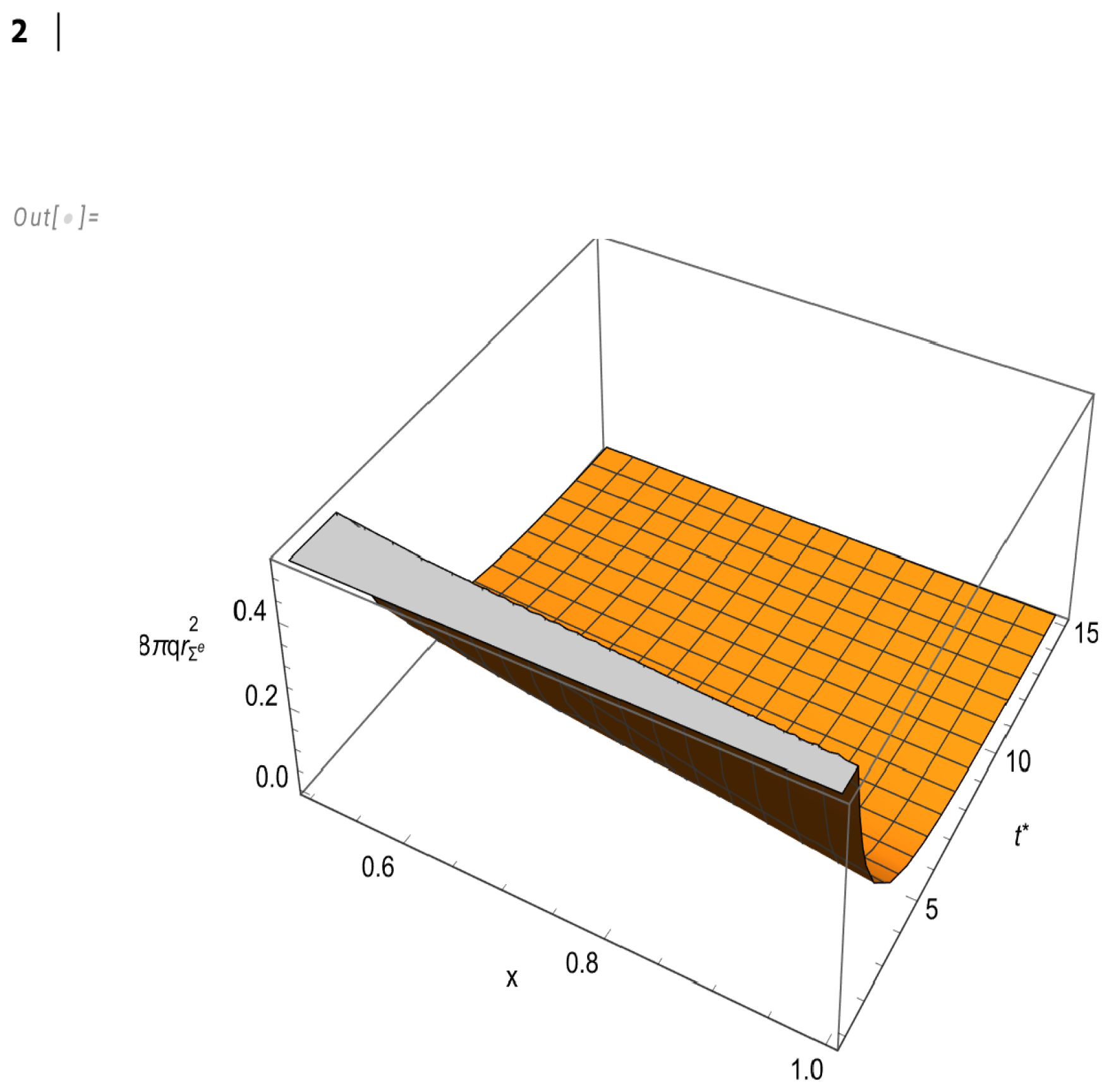
The behavior of the physical variables is depicted in Figure 2 and Figure 3. The graphics for and q have been drawn for the variables and x in the intervals and respectively. Instead, for we have chosen the intervals and in order to better illustrate the appearance of the region of negative energy-density. The fast convergence of the system to the static regime is well illustrated in Figure 3.
5. Discussion
The main purpose of this work has been to exhibit the viability of the formation of a ghost star as the end point of the evolution of a self–gravitating fluid distribution. To achieve this goal we have presented an analytical model of a dissipative spherically symmetric fluid distribution evolving toward a ghost star.
We have initially found a primeval solution satisfying the vanishing complexity factor condition, the quasi–homologous evolution and . This primeval solution was next modified to satisfy the required asymptotic conditions (66). Finally we have chosen the remaining arbitrary functions to fully specify our model. This final model represents and expanding fluid distribution endowed with a cavity surrounding the center, tending to a static configuration. The endpoint of the evolution of this model is a ghost star as illustrated by Figure 1.
Furthermore, in the limit we have , implying, because of (12), the vanishing of the four-acceleration of the fluid forming the ghost star (which explains the vanishing of the “thermal inertial term” mentioned before). This implies in its turn, according to (A1), that the gravitational term in the dynamic equation (A2) (the Tolman mass [33]) vanishes, and the equilibrium is reached by the balance between the radial pressure gradient and the anisotropic factor. A particular model of a ghost star with vanishing complexity factor and vanishing Tolman mass has been considered in [1].
The model satisfies asymptotically Darmois conditions on the external boundary surface, whereas on the inner boundary surface such conditions are not satisfied indicating thereby the appearance of shells on this hypersurface. The presence of these thin shells are likely to be produced by the simplicity of the model. More involved analytical models, or numerical models could avoid these “drawbacks”.
We should recall that the very existence of ghost stars relies on the assumption of the existence of regions of the fluid distribution endowed with negative energy-density. In this respect it should be mentioned that negative energy-density (or negative mass) is a subject extensively considered in the literature (see [34,35,36,37,38,39,40,41,42,43,44,45,46,47,48,49] and references therein). Particularly relevant are those references relating the appearance of negative energy-density with quantum effects.
It is worth mentioning the relevance of the observational aspects of the ghost stars, in general and of our model in particular. On the one hand it is evident that the shadow of such kind of object should differ from the one produced by a self-gravitating star with non-vanishing total mass. In the particular case of the model here considered one should be able to detect the variation of the shadow as the system approaches the state of ghost star. We ignore if the ongoing observations of this kind [50,51,52,53] are able to do that, but this is an important issue to consider. A research endeavor pointing in a similar direction has been recently published in [54].
On the other hand, it is worth noticing that ghost stars are a sort of reservoirs of dark mass produced by the appearance of negative energy-density is some regions of the fluid distribution. It remain to be seen if the general problem of dark matter could be, at least partially, be explained in terms of ghost stars [55].
We would also like to mention that an important piece of theoretical evidence behind the concept of ghost star is still missing. We have in mind a microscopic theory accounting for the appearance of negative energy-density. Research in this direction could provide further support to the astrophysical relevance of ghost stars.
Finally, let us mention two natural extensions of the work here presented
- We have resorted to GR to describe the gravitational interaction. It would be interesting to consider the same problem within the context of one of the extended gravitational theories [60].
Author Contributions
All authors contributed equally to this work. All authors have read and agreed to the published version of the manuscript. Conceptualization, L.H.; methodology, L.H., A.D.P.; J.O. ; software, J. O.; formal analysis, L.H., A.D. P.; J. O.; writing—original draft preparation, L. H. writing—review and editing, L. H:; A.D. P.; J. O.; funding acquisition, L. H.; J.O.; All authors have read and agreed to the published version of the manuscript.
Funding
This work was partially supported by the Grant PID2021-122938NB-I00 funded by MCIN/AEI/ 10.13039/501100011033 and by ERDF A way of making Europe, as well as the Consejería de Educación of the Junta de Castilla y León under the Research Project Grupo de Excelencia Ref.:SA097P24 (Fondos Feder y en línea con objetivos RIS3).
Institutional Review Board Statement
Not applicable.
Informed Consent Statement
Not applicable.
Data Availability Statement
Not applicable.
Conflicts of Interest
The authors declare no conflict of interest. The funders had no role in the design of the study; in the collection, analyses, or interpretation of data; in the writing of the manuscript, or in the decision to publish the results.
Appendix A Dynamical Equation
which allows to write the dynamical equation following from the Bianchi identities as (see [9] for details)
References
- Herrera, L.; Di Prisco, A.; Ospino, J. Ghost stars in general relativity. Symmetry 2024, 16, 562. [Google Scholar] [CrossRef]
- Zeldovich, Ya.B.; Novikov, I.D. Relativistic Astrophysics. Vol I. Stars and Relativity; University of Chicago Press: Chicago, Illinois. USA, 1971. [Google Scholar]
- Zeldovich, Ya.B. The Collapse of a Small Mass in the General Theory of Relativity. Sov. Phys. JETP 1962, 15, 446. [Google Scholar]
- Herrera,L. ; Ponce de Leon, J. Confined gravitational fields produced by anisotropic spheres. J. Math. Phys. 1985, 26, 2847–2849. [Google Scholar] [CrossRef]
- Herrera, L.; Di Prisco, A.; Ospino, J. Non-static fluid spheres admitting a conformal Killing vector: Exact solutions. Universe 2022, 8, 296. [Google Scholar] [CrossRef]
- Naseer, T.; Hassan, K.; Sharif, M. Possible existence of ghost stars in the context of electromagnetic field. Chin. J. P. 2025, 94, 594. [Google Scholar] [CrossRef]
- Herrera, L.; Di Prisco, A.; Ospino, J. Evolution of Self-Gravitating Fluid Spheres Involving Ghost Stars. Symmetry 2024, 16, 1422. [Google Scholar] [CrossRef]
- Herrera, L. New definition of complexity for self–gravitating fluid distributions: The spherically symmetric static case. Phys. Rev. D 2018, 97, 044010. [Google Scholar] [CrossRef]
- Herrera, L.; Di Prisco, A.; Ospino, J. Definition of complexity for dynamical spherically symmetric dissipative self–gravitating fluid distributions. Phys. Rev. D 2018, 98, 104059. [Google Scholar] [CrossRef]
- Herrera, L.; Di Prisco, A.; Ospino, J. Quasi–homologous evolution of self–gravitating systems with vanishing complexity factor. Eur. Phys. J. C 2020, 80, 631. [Google Scholar] [CrossRef]
- L. Herrera, G. L. Herrera, G. Le Denmat and N.O. Santos. Cavity evolution in relativistic self–gravitating fluids. Class. Quantum Grav. 2010. [Google Scholar]
- Schwarzschild, M. Structure and Evolution of the Stars; Dover: New York, NY, USA, 1958. [Google Scholar]
- Hansen, C.; Kawaler, S. Stellar Interiors: Physical Principles, Structure and Evolution; Springer: Berlin/Heidelberg, Germany, 1994. [Google Scholar]
- Kippenhahn, R.; Weigert, A. Stellar Structure and Evolution; Springer: Berlin/Heidelberg, Germany, 1990. [Google Scholar]
- Liddle, A. R.; Wands, D. Microwave background constraints on extended inflation voids. Mon. Not. R. Astron. Soc. 1991, 253, 637. [Google Scholar] [CrossRef]
- Peebles, P. J. E. The Void Phenomenon. Astrophys. J. 2001, 557, 445. [Google Scholar] [CrossRef]
- Misner, C.; Sharp, D. Relativistic Equations for Adiabatic, Spherically Symmetric Gravitational Collapse. Phys. Rev. 1964, 136, B571. [Google Scholar] [CrossRef]
- Cahill, M.; McVittie, G. Spherical Symmetry and Mass-Energy in General Relativity. I. General Theory. J. Math. Phys. 1970, 11, 1382. [Google Scholar] [CrossRef]
- Darmois, G. Memorial des Sciences Mathematiques; Gauthier-Villars: Paris, France, (1927); p. 25.
- Chan, R. Collapse of a radiating star with shear. Mon. Not. R. Astron. Soc. 1997, 288, 589–595. [Google Scholar] [CrossRef]
- Israel,W. Singular hypersurfaces and thin shells in general relativity. Il Nuovo Cimento B 1966, 10, 1. [Google Scholar]
- Israel, W. Nonstationary irreversible thermodynamic: A causal relativistic theory. Ann. Phys. (NY) 1976, 100, 310–331. [Google Scholar] [CrossRef]
- Israel, W.; Stewart, J. Thermodynamic of nonstationary and transient effects in a relativistic gas. Phys. Lett. A 1976, 58, 213–215. [Google Scholar] [CrossRef]
- Israel, W.; Stewart, J. Transient relativistic thermodynamics and kinetic theory. Ann. Phys. (NY) 1979, 118, 341–372. [Google Scholar] [CrossRef]
- Eckart, C. The Thermodynamics of Irreversible Processes. III. Relativistic Theory of the Simple Fluid. Phys. Rev. 1940, 58, 919. [Google Scholar] [CrossRef]
- Landau, L.; Lifshitz, E. Fluid Mechanics, Pergamon Press: London, U. K. 1959.
- Cattaneo, C. Sulla conduzione del calore. Atti Sem. Mat. Fiz. Univ. Modena 1948, 3, 83–101. [Google Scholar]
- Cattaneo, C. Sur une forme de l’equation de la chaleur eliminant le paradoxe d’une propagation instantanee. Compt. R. Acad. Sci. Paris 1958, 247, 431–433. [Google Scholar]
- Vernotte, P. Les paradoxes de la theorie continue de l’equation de la chaleur. Compt. R. Acad. Sci. Paris 1958, 246, 3154–3155. [Google Scholar]
- Triginer, J.; Pavon, D. On the thermodynamics of tilted and collisionless gases in Friedmann–Robertson–Walker spacetimes. Class. Quantum Grav. 1995, 12, 199. [Google Scholar] [CrossRef]
- M. K. ( 1985.
- Tolman, R. On the weight of heat and thermal equilibrium in general relativity. Phys. Rev 1930, 35, 904. [Google Scholar] [CrossRef]
- Tolman, R. On the use of the energy-momentum principle in general relativity. Phys. Rev 1930, 35, 875. [Google Scholar] [CrossRef]
- Bondi, H. Negative Mass in General Relativity. Rev. Mod. Phys. 1957, 29, 423–428. [Google Scholar] [CrossRef]
- Cooperstock, F.I.; Rosen, N. A nonlinear gauge-invariant field theory of leptons. Int. J. Theor. Phys. 1989, 28, 423–440. [Google Scholar] [CrossRef]
- Bonnor, W.B.; Cooperstock, F.I. Does the electron contain negative mass? Phys. Lett. A. 1989, 139, 442–444. [Google Scholar] [CrossRef]
- Papapetrou, A. Lectures on General Relativity; D. Reidel, Dordrecht-Holland: Boston. USA, 1974. [Google Scholar]
- Herrera, L.; Varela, V. Negative energy density and classical electron models. Physics Letters A, 1994, 189, 11–14. [Google Scholar] [CrossRef]
- Najera, S.; Gamboa, A.; Aguilar-Nieto, A.; Escamilla-Rivera, C. On Negative Mass Cosmology in General Relativity. arXiv: 2105.110041v1, arXiv:2105.110041v1 2021.
- Farnes, J.S. A unifying theory of dark energy and dark matter: Negative masses and matter creation within a modified λ cdm framework. Astron. Astrophys. 2018, 620, A92. [Google Scholar] [CrossRef]
- Maciel, A.; Delliou, M.L.; Mimoso, J.P. New perspectives on the TOV equilibrium from a dual null approach. Class. Quantum Gravity 2020, 37, 125005. [Google Scholar] [CrossRef]
- Herrera, L. Nonstatic hyperbolically symmetric fluids. Int. J. Mod. Phys. D 2022, 31, 2240001. [Google Scholar] [CrossRef]
- Capozziello, S.; Lobo, F.S.N.; Mimoso, J.P. Energy conditions in modified gravity. Phys. Lett. B 2014, 730, 280–283. [Google Scholar] [CrossRef]
- Capozziello, S.; Lobo, F.S.N.; Mimoso, J.P. Generalized energy conditions in extended theories of gravity. Phys. Rev. D 2015, 91, 124019. [Google Scholar] [CrossRef]
- Barcelo, C.; Visser, M. Twilight for the Energy Conditions? Int. J. Mod. Phys. D 2002, 11, 1553–1560. [Google Scholar] [CrossRef]
- Kontou, E.A.; Sanders, K. Energy conditions in general relativity and quantum field theory. Class. Quantum Gravity 2020, 37, 193001. [Google Scholar] [CrossRef]
- Pavsic, M. On negative energies, strings, branes, and braneworlds: A review of novel approaches. Int. J. Mod. Phys. A 2020, 35, 2030020. [Google Scholar] [CrossRef]
- Chen-Hao Hao etal. Emergence of negative mass in general relativity. Eur. Phys. J. C 2024, 84, 878. [Google Scholar] [CrossRef]
- Bormashenko, E. The effect of negative mass in gravitating systems. Pramana J. P. 2023, 97, 199. [Google Scholar] [CrossRef]
- Akiyama, K. et al. (Event Horizon Telescope Collaboration). First M87 Event Horizon Telescope Results. I. The Shadow of the Supermassive Black Hole. Astrophys. J. Lett. 2019, 875, L1. [Google Scholar]
- Akiyama, K. et al. (Event Horizon Telescope Collaboration). First Sagittarius A Event Horizon Telescope Results. I. The Shadow of the Supermassive Black Hole in the Center of the Milky Way. Astrophys. J. Lett. 2022, 930, L12. [Google Scholar]
- Psaltis, D. Testing general relativity with the Event Horizon Telescope. Gen. Relativ. Gravit. 2019, 51, 137. [Google Scholar] [CrossRef]
- Gralla, S. E. Can the EHT M87 results be used to test general relativity? Phys. Rev. D 2021, 103, 024023. [Google Scholar] [CrossRef]
- Nalui, S.; Bhattacharya, S. Herrera complexity and shadows of spherically symmetric compact objects. Phys. Lettt. B 2025, 861, 139261. [Google Scholar] [CrossRef]
- Croon, D.; Sevillano Munoz. , S. Repository for extended dark matter object constraints. Eur.Phys J. C 2025, 85, 8. [Google Scholar] [CrossRef] [PubMed]
- Thirukkanesh, S; Maharaj, S. D. Radiating relativistic matter in geodesic motion. J. Math. Phys. 2009, 50, 022502. [Google Scholar] [CrossRef]
- Thirukkanesh, S.; Maharaj, S. D. Mixed potentials in radiative stellar collapse. J. Math. Phys. 2010, 51, 072502. [Google Scholar] [CrossRef]
- Ivanov, B. All solutions for geodesic anisotropic spherical collapse with shear and heat radiation. Astrophys. Space Sci. 2016, 361, 18. [Google Scholar] [CrossRef]
- Ivanov, B. A different approach to anisotropic spherical collapse with shear and heat radiation. Int. J. Mod. Phys. D 2016, 25, 1650049. [Google Scholar] [CrossRef]
- Capozziello, S.; Laurentis, M.D. Extended theories of gravity. Phys. Rep. 2011, 509, 167. [Google Scholar] [CrossRef]
Figure 1.
, evaluated at , as function of x in the interval ; and as functions of .
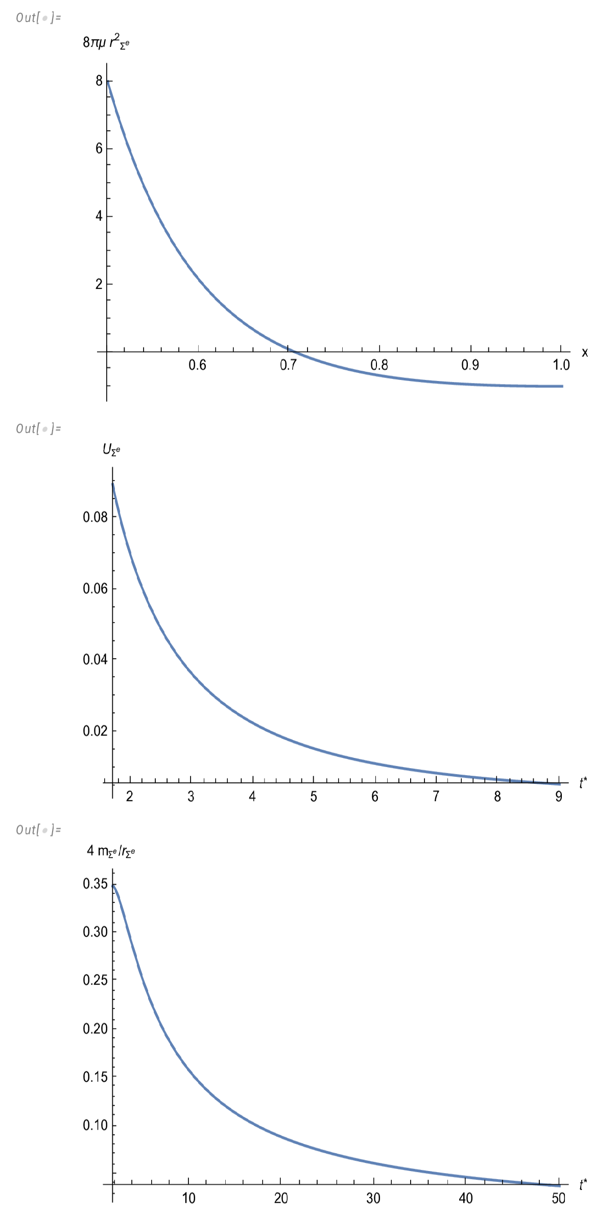
Figure 2.
, and as functions of x and .
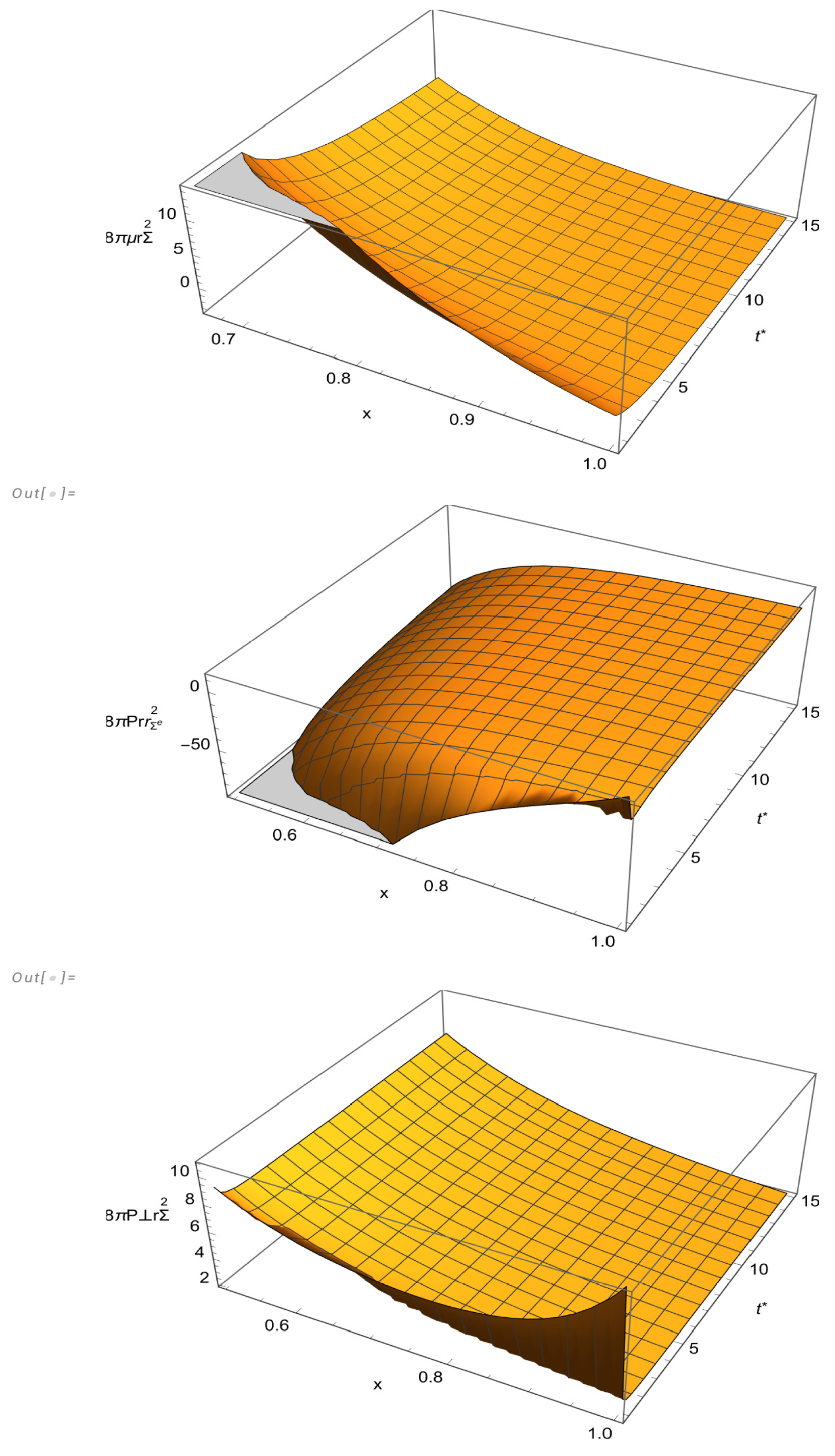
Figure 3.
as function of x and .
Disclaimer/Publisher’s Note: The statements, opinions and data contained in all publications are solely those of the individual author(s) and contributor(s) and not of MDPI and/or the editor(s). MDPI and/or the editor(s) disclaim responsibility for any injury to people or property resulting from any ideas, methods, instructions or products referred to in the content. |
© 2025 by the authors. Licensee MDPI, Basel, Switzerland. This article is an open access article distributed under the terms and conditions of the Creative Commons Attribution (CC BY) license (http://creativecommons.org/licenses/by/4.0/).
Copyright: This open access article is published under a Creative Commons CC BY 4.0 license, which permit the free download, distribution, and reuse, provided that the author and preprint are cited in any reuse.


