
Submitted:
18 September 2024
Posted:
18 September 2024
You are already at the latest version
Abstract
We present some exact analytical solutions describing, either the evolution of fluid distributions corresponding to a ghost star (vanishing total mass), or describing the evolution of fluid distributions which attain the ghost star status at some point of their lives. The first two solutions correspond to the former case, they admit a conformal Killing vector (CKV) and describe the adiabatic evolution of a ghost star. Other two solutions corresponding to the latter case are found, which describe evolving fluid sphere absorbing energy from the outside, leading to a vanishing total mass at some point of their evolution. In this case the fluid is assumed to be expansion–free. In all four solutions the condition of vanishing complexity factor was imposed. A discussion of the physical implications of the results, is presented.
Keywords:
Relativistic fluids
; interior solutions
; spherically symmetric sources
1. Introduction
In a recent paper [1] we have explored the possibility of finding fluid distributions of anisotropic fluids whose total mass is zero [2,3,4]. Such configurations which we named ghost stars, are characterized by negative energy-density in some regions of the distribution, producing a vanishing total mass. The solutions presented in [1] are static, and may be regarded as either the final or the initial state of a dynamical process.
In this work we endeavor to describe the evolution of fluid distributions describing the following possible scenarios
- The adiabatic evolution of a ghost star. The total mass remains zero all along the evolution.
- The non–adiabatic evolution of fluid distribution reaching at some point a zero total mass (with non–vanishing energy density).
For the first scenario we obtain two solutions admitting a CKV. One of them corresponds to a CKV orthogonal to the four–velocity vector of the fluid, whereas the other admits a CKV parallel to the four–velocity.
The motivation behind the admittance of CKV is provided by the fact that it generalizes the well known concept of self–similarity, which play a very important role in classical hydrodynamics [5,6,7].
Indeed, self-similarity is to be expected whenever the system under consideration possesses no characteristic length scale [8]. This includes the study of systems close to the critical point, where the correlation length becomes infinite, allowing the coexistence of different phases of the fluid (e.g., liquid–vapor), the phase boundaries vanish and density fluctuations occur at all length scales. Also it has been proved to be useful in the study of strong explosions and thermal waves [9,10,11,12].
This explains the great interest aroused by this kind of symmetry since the pioneering work by Cahill and Taub [13], for further developments in the last decade see, for example, [14,15,16,17,18,19,20,21,22,23,24,25,26,27,28,29,30,31,32,33,34,35,36,37,38,39,40,41,42] and references therein.
This first couple of solutions represents fluid distributions contracting from arbitrarily large areal radius to compact fluid distribution with finite areal radius, or fluid distributions expanding from some finite value of the areal radius to infinity, always satisfying the vanishing total mass condition. The Darmois conditions at the boundary are satisfied, and as expected the energy density is negative in some regions of the fluid distribution.
In the second scenario both solutions satisfy the vanishing expansion scalar condition. The interest generated by such a condition stems from the fact that it implies the appearance of a cavity around the center, thereby bringing out its potential relevance in the modeling, among other phenomena, of voids observed at cosmological scales [43,44]. The study of expansion–free fluids started with the paper by V. Skripkin, describing the evolution of a spherically symmetric distribution of incompressible non–dissipative fluid, following a central explosion [45] (see also [46]).
Later on, a general study on shearing expansion-free spherical fluid evolution (including pressure anisotropy) was carried out in [47], where the unavoidable appearance of a cavity surrounding the center in expansion–free solutions was explained as consequence of the fact that the condition requires that the innermost shell of fluid should be away from the centre, initiating therefrom the formation of a cavity.
Newest results (in the last decade or so) regarding expansion–free fluids may be found in [48,49,50,51,52,53,54,55,56,57,58,59,60,61,62,63,64,65] and references therein.
The two solutions satisfying the expansion–free condition represent fluid distribution contracting from arbitrarily large configurations to a singularity. They evolve absorbing energy from the outside, and at some point of their evolutions their total mass vanishes. Thus the solutions pass through a ghost star state.
All solutions will be found by imposing additional restrictions allowing the full integration of field equations. Some of these restrictions are endowed with a distinct physical meaning, while others concern specific choices of the parameters. Among the former stand out the vanishing complexity factor condition as defined in [66,67] and the quasi–homologous evolution [68]. A discussion on all the presented models is brought out in the last section.
2. The Relevant Equations and Variables
The system we are dealing with consists in a spherically symmetric distribution of collapsing fluid, bounded by a spherical surface . The fluid is assumed to be locally anisotropic (principal stresses unequal) and undergoing dissipation in the form of heat flow (diffusion approximation). We shall proceed now to summarize the definitions and main equations required for describing spherically symmetric dissipative fluids. A detailed description may be found in [68].
2.1. The Metric, the Energy–Momentum Tensor, the Kinematic Variables and the Mass Function
Choosing comoving coordinates, the general interior metric can be written as
where A, B and R are functions of t and r and are assumed positive. We number the coordinates , , and . Observe that A and B are dimensionless, whereas R has the same dimension as r.
The energy momentum tensor in the canonical form, reads
with
where is the energy density, the radial pressure, the tangential pressure, the heat flux, the four–velocity of the fluid, and a unit four–vector along the radial direction. For comoving observers, we have
satisfying
Both bulk and shear viscosity, as well as dissipation in the free streaming approximation can be trivially absorbed in , and q.
The acceleration and the expansion of the fluid are given by
and its shear by
From the equations above we have for the four–acceleration and its scalar a,
and for the expansion
while for the shear we obtain
where
in the above prime stands for r differentiation and the dot stands for differentiation with respect to t.
Introducing the proper time derivative given by
we can define the velocity U of the collapsing fluid as the variation of the areal radius with respect to proper time, i.e.
where R defines the areal radius of a spherical surface inside the fluid distribution (as measured from its area).
Then (11) can be rewritten as
An, alternative expression for m may be found using field equations, it reads
satisfying the regular condition .
From the above equation it follows that, since in order to avoid shell crossing singularities, the vanishing total mass condition () requires that the “effective energy- density” () should be either zero (the trivial case), or changes its sign within the fluid distribution (ghost star).
2.2. The Complexity Factor
The solutions exhibited in the next section satisfy the condition of vanishing complexity factor. This is a scalar function intended to measure the degree of complexity of a given fluid distribution [66,67], and is related to the so called structure scalars [71].
As shown in [66,67] the complexity factor is identified with the scalar function which defines the trace–free part of the electric Riemann tensor (see [71] for details).
Then after lengthy but simple calculations, using field equations we obtain [72]
It is worth noticing that due to a different signature, the sign of in the above equation differs from the sign of the used in [66] for the static case.
In terms of the metric functions the scalar reads
2.3. The Homologous and Quasi–Homologous Conditions
In the dynamic case, the discussion about the complexity of a fluid distribution involves not only the complexity factor which describes the complexity of the structure of the fluid, but also the complexity of the pattern of evolution.
Following previous works [67,68] we shall consider two specific modes of evolution as the most suitable candidates to describe the simplest pattern of evolution. These are, the homologous evolution (H) [67] characterized by
and
where and denote the areal radii of two concentric shells () described by , and , respectively.
2.4. The exterior spacetime and junction conditions
Since our fluid distribution is bounded we assume that outside the space–time is described by Vaidya metric which reads.
where denotes the total mass, and v is the retarded time.
The smooth matching of the full nonadiabatic sphere to the Vaidya spacetime, on the surface constant, requires the fulfillment of the Darmois conditions, i.e. the continuity of the first and second fundamental forms across (see [73] and references therein for details), which implies
and
where means that both sides of the equation are evaluated on .
If the above conditions are not satisfied then we have to assume the presence of a thin shell on the boundary surface.
2.5. The Transport Equation
In the case of non–adiabatic evolution we have to resort to some transport equation to describe the evolution and spatial distribution of the temperature. Thus for example within the context of the Israel– Stewart theory [74,75,76] the transport equation for the heat flux reads
where denotes the thermal conductivity, and T and denote temperature and relaxation time respectively.
In the spherically symmetric case under consideration, the transport equation has only one independent component which may be obtained from (24) by contracting with the unit spacelike vector , we get
3. Exact Solutions
We shall now proceed to present exact analytical solutions describing two different scenarios,
- the evolution of a ghost star keeping its nature () all along its evolution
- the evolution of a compact object (not a ghost star) attaining the ghost star condition at some moment of its life.
We shall consider, both, the non–dissipative and the dissipative case.
In order to specify our models we need to impose some further restrictions. In this work such restriction will be
-
The admittance of a conformal killing vector (CKV),or
- The expansion–free condition.
In some cases the above conditions have to be complemented with additional restrictions such as
- The vanishing complexity factor condition.
- The homologous or the quasi–homologous approximation.
3.1. Solutions admitting a CKV
In this subsection we shall consider spacetimes satisfying the equation
where denotes the Lie derivative with respect to the vector field , which unless specified otherwise, has the general form
and in principle is a function of t and r. The case corresponds to a homothetic Killing vector (HKV). The solutions described here are particular cases of solutions found in [27].
We shall consider two possible subclasses, both of which describe non–dissipative evolution
- orthogonal to ,
- parallel to .
In the first case ( orthogonal to ), we shall obtain from the matching conditions, the QH condition and the vanishing complexity factor condition, with , solution I.
In the second case ( parallel to ), we shall obtain from the matching conditions and the vanishing complexity factor condition, solution .
Let us start by considering the case orthogonal to , and .
3.1.1. Solution I:
In this case we obtain from (27) (see [27] for details)
where f and g are two arbitrary functions of their arguments and is a unit constant with dimensions of .
Thus any model is determined up to three arbitrary functions , in terms of which the field equations read
Since (33) is just the first integral of (34), boundary conditions provide only one additional equation.
In order to specify a solution we still need to impose two additional conditions.
One of these conditions will be the quasi–homologous condition which implies because of (20) that the fluid is shear–free (), implying in its turn
Thus the metric functions become
In order to determine , we shall further impose the vanishing complexity factor condition (), producing
with , and is another integration constant.
Thus, the corresponding physical variables read
The graphics of these physical variables for the solution I are given in Figure 1.
Solution I describes an expanding sphere, whose initial boundary areal radius grows from at , to infinity as , and a contracting sphere whose boundary areal radius decreases from infinity at to at . This picture repeating each time interval , for any positive real integer n.
In order to determine the regions of the fluid distribution where the energy density is negative (required to have a vanishing total mass) we shall write the condition from (40) in the form
whose solution reads
with and .
The curve in Figure 2 is formed by all points in the plane where the energy-density vanishes. The curve divides the plane in two regions, corresponding to negative and positive values of . As is apparent from the graphic of in Figure 1, these regions are denoted by A and B respectively, in Figure 2.
3.1.2. Solution II:
We shall next analyze the case when the CKV is parallel to the four–velocity vector in the absence of dissipation. In this case the equation (27) produces
where is an arbitrary function of its argument and . It is worth noticing that in this case the fluid is necessarily shear–free, implying thereby that it evolves in QH regime.
Thus the line element may be written as
Next, using (45) and the field equations, the condition reads (see [27] for details)
whose solution is
implying
where g and f are two arbitrary functions of their argument.
Thus the metric is defined up to three arbitrary functions ().
Indeed, evaluating the mass function at the boundary surface we obtain from (22) and (48)
where
and
with .
Thus assuming , equation (50) becomes
Solutions to the above equation in terms of elementary functions may be obtained by assuming , in which case a possible solution to (54) is
which exhibits the same time dependence as in solution I.
Thus, as in the previous model, solution describes an expanding sphere, whose initial boundary areal radius grows from at , to infinity as , and a contracting sphere whose boundary areal radius decreases from infinity at to at . This picture repeating each time interval , for any positive real integer n.
Imposing further the vanishing complexity factor condition, then functions are given by
The physical variables corresponding to this solution read
The behavior of these physical variables is depicted in Figure 3.
From the definition of the mass function (11), using (48), (49) (55) and (56), the condition implies
The above equation is satisfied for any value of t if and , which, as expected, are the same relationships which follow from (51) and (56).
In oder to determine the regions of the fluid distribution where the energy density is negative (required to have a vanishing total mass) we shall write the condition from (57) in the form
whose solution reads
where , .
The graphic of z as function of y is plotted in Figure 4. The curve contains all the points of the plane where the energy-density vanishes, and divides the plane in two regions (A and B) corresponding to negative and positive energy-density respectively.
3.2. Expansion–Free Models
We shall now present two models satisfying the vanishing expansion condition.
We recall that under such a condition the line element may be written as (see [65] for details)
where is a unit constant with dimensions .
Besides, as is known, the expansion-free models present an internal vacuum cavity surrounding the center, implying that we have not to worry about regularity conditions of the solution at the center of symmetry.
These solutions will be found by imposing additional restrictions allowing the full integration of the field equations, among which the vanishing complexity factor condition and the quasi-homologous evolution are the most relevant.
3.2.1. Solution III: , ,
For this model, we shall complement the expansion–free condition with the vanishing complexity factor condition , and we shall assume that A only depends on the radial coordinate, and R is a separable function (i.e., ).
From all these conditions the general form of the metric variables read (see [65] for details)
where and are dimensionless constants and and are constants with dimensions and , respectively.
Let us choose for our model
Then the expression for the mass function evaluated at the boundary surface and the areal radius of the boundary surface become
and
where and we have put .
From (68) it follows that the total mass vanishes at .
The physical variables for this model read
where the expression above for the temperature has been obtained using the truncated transport equation (26), and .
The “effective energy–density” appearing in the definition of the mass function (15) evaluated at reads
Figure 5 and Figure 6 depict the behavior of physical variables, the radial distribution of the “effective energy–density” at , when the total mass vanishes, and the evolution of the total mass.
The model represents a contracting sphere with initial negative mass absorbing energy through the boundary surface. At the total mass vanishes becoming positive afterward.
It is worth mentioning that although the total mass tends to zero as , the fluid distribution does not characterize a ghost star in that limit, since in such a case the total mass tends to zero due to the fact that the integrand in (15) tends to zero as , and not because of change of sign of the effective energy-density as is the case for a ghost star.
3.2.2. ,
We shall now consider geodesic fluids, for which we have
the above condition together with the expansion-free condition
plus the condition , produces
where is an arbitrary function of its argument with dimensions .
For our model we shall choose
producing
where
and the mass function becomes
From (82) evaluated at we see that at , being negative before that time and becoming positive afterward.
For this metric, the physical variables and the shear read as follows:
where, as in the previous case, the temperature has been calculated using the truncated transport equation (26).
Figure 7 and Figure 8 depict the behavior of physical variables, the radial distribution of the “effective energy–density” at , when the total mass vanishes, and the evolution of the total mass.
The model represents a contracting sphere with initial negative mass absorbing energy through the boundary surface. At the total mass vanishes becoming positive afterward. From the above it follows that
Evaluating the above expression at we see that it changes of sign within the fluid distribution, thereby explaining the vanishing of the total mass at (see Figure 8).
4. Discussion
We have presented a set of solutions of fluid spheres whose evolution involves ghost stars.
The first two solutions represent the adiabatic evolution of a ghost star, they admit a CKV which may be either orthogonal or parallel to the four-velocity vector. These solutions (I and ) describe either an expanding sphere, with an initial boundary areal radius growing from some finite value to infinity, or a contracting sphere whose boundary areal radius decreases from infinity to some finite final value. In both cases at all times and the energy–density is negative in some regions of the fluid distributions (see Figure 2 and 4). The full description of these models is provided by equations (38-42), and (55-60) for models I and respectively. Their behavior is depicted in Figure 1, 2, 3, 4.
In both cases the vanishing complexity factor condition applies and the solutions match smoothly to the Minkowski space-time on the boundary surface of the fluid distribution.
The second couple of solutions satisfies the expansion-free condition and the vanishing complexity factor condition. In one case (solution ), these last conditions are complemented with the assumption that and R is a separable function. In the last case (solution ) we assume the fluid to be geodesic.
The full description of model is provided by Equations (64–75) and illustrated in Figure 5 and 6. It describes a collapsing fluid whose total mass evolves from negative values to positive ones by absorbing radiation. At some point of the evolution () the total mass vanishes becoming positive afterward. At the effective energy–density is negative in some regions of the fluid distributions as shown in Figure 6.
This rather unusual scenario (compact object absorbing radiation), has been invoked in the past to explain the origin of gas in quasars [78]. A semi-numerical example for such a model is described in [79].
Finally, the last model is geodesic (solution IV) and satisfies, besides the expansion–free condition, the vanishing complexity factor condition. It is described by Equations (80–88). This solution depicts a collapsing fluid for which as , the energy density and the radial pressure diverge and satisfy the equation of the state , whereas the heat flux vector and the tangential pressure vanish, and the temperature tends toward . As it happens in Solution , at some point of its evolution the total mass vanishes, and as expected the effective energy–density is negative in some regions of the fluid distributions as shown in Figure 8.
Unlike solutions , solutions do not satisfy Darmois conditions on the boundary surface, implying that these surfaces are thin shells.
It is worth recalling that the very existence of ghost stars relies on the presence of negative energy–density (the effective energy–density in the non–adiabatic case). Negative energy-density (mass) has a long and a venerable history in general relativity, both at classical level as well as in the quantum level (see [80,81,82,83,84,85,86,87,88,89,90,91,92,93,94] and references therein).
An issue requiring much more research work concerns the possibility to observe a ghost star. We have in mind either a “permanent” ghost star as the case described by solutions I and , or a compact object attaining momentarily the ghost star status, as the two models described by solutions and .
At present we contemplate two possible ways to establish (or dismiss) the very existence of a ghost star. On the one hand, by observing the shadow of such objects following the line of research open by the Event Horizon Telescope (EHT) Collaboration (see [95,96,97,98] and references therein). On the other hand the formation of a ghost star, even if for a short time interval, involves radiating processes whose observation could help to identify a ghost star.
In relationship with this last point it would be very helpful to find an evolving model , with a positive energy flux at the boundary surface, leading asymptotically to a ghost star. Unfortunately, neither of the solutions presented here satisfy such a condition.
Author Contributions
All authors contributed equally to this work. All authors have read and agreed to the published version of the manuscript. Conceptualization, L.H.; methodology, L.H., A.D.P.; J.O. ; software, J. O.; formal analysis, L.H., A.D. P.; J. O.; writing—original draft preparation, L. H. writing—review and editing, L. H:; A.D. P.; J. O.; funding acquisition, L. H.; J.O.; All authors have read and agreed to the published version of the manuscript.
Funding
This work was partially supported by the Spanish Ministerio de Ciencia, Innovación, under Research Project No. PID2021-122938NB-I00.
Institutional Review Board Statement
Not applicable.
Informed Consent Statement
Not applicable.
Data Availability Statement
Not applicable.
Conflicts of Interest
The authors declare no conflict of interest. The funders had no role in the design of the study; in the collection, analyses, or interpretation of data; in the writing of the manuscript, or in the decision to publish the results.
Appendix A. Einstein equations
Einstein’s field equations for the interior spacetime (1) are given by
and its non zero components read
References
- Herrera, L.; Di Prisco, A.; Ospino, J. Ghost stars in general relativity. Symmetry 2024, 16, 562. [Google Scholar] [CrossRef]
- Zeldovich, Ya.B.; Novikov, I.D. Relativistic Astrophysics. Vol I. Stars and Relativity; University of Chicago Press: Chicago, IL, USA, 1971. [Google Scholar]
- Zeldovich, Ya.B. The Collapse of a Small Mass in the General Theory of Relativity. Sov. Phys. JETP 1962, 15, 446. [Google Scholar]
- Herrera, L; Ponce de Leon, J. Confined gravitational fields produced by anisotropic spheres. J. Math. Phys. 1985, 26, 2847–2849. [Google Scholar] [CrossRef]
- Schwarzschild, M. Structure and Evolution of the Stars; Dover: New York, NY, USA, 1958. [Google Scholar]
- Hansen, C.; Kawaler, S. Stellar Interiors: Physical Principles, Structure and Evolution; Springer: Berlin/Heidelberg, Germany, 1994. [Google Scholar]
- Kippenhahn, R.; Weigert, A. Stellar Structure and Evolution; Springer: Berlin/Heidelberg, Germany, 1990. [Google Scholar]
- Barenblatt, G.I.; Zeldovich, Ya.B. Self-Similar Solutions as Intermediate Asymptotics. Ann. Rev. Fluid. Mech. 1972, 4, 285–312. [Google Scholar] [CrossRef]
- Sedov, L. I. Propagation of strong shock waves. J. Appl. Math. Mech. 1946, 10, 241–250. [Google Scholar]
- Sedov, L. I. Similarity and Dimensional Methods in Mechanics; Academic. New York, USA, 1967.
- Taylor, G.I. The Formation of a Blast Wave by a Very Intense Explosion. II. The Atomic Explosion of 1945. Proc. Roy. Soc. 1950, 201, 175–186. [Google Scholar]
- Zeldovich, Ya.B.; Raizer, Yu.P. Physics of Shock Waves and High Temperature; Academic. New York, USA, 1963.
- Cahill, M.E.; Taub, A.H. Spherically symmetric similarity solutions of the Einstein field equations for a perfect fluid. Commun. Math. Phys. 1971, 21, 1–40. [Google Scholar] [CrossRef]
- Bhar, P. Vaydya–Tikekar–type superdense star admitting conformal motion in presence of quintessence field. Eur. Phys. J. C 2015, 75, 123. [Google Scholar] [CrossRef]
- Apostolopoulos, P.S. Spatially inhomogeneous and irrotational geometries admitting intrinsic conformal symmetries. Phys. Rev. D 2016, 94, 124052. [Google Scholar] [CrossRef]
- Shee, D.; Rahaman, F.; Guha, B.K.; Ray, S. Anisotropic stars with non–static conformal symmetry. Astr. Space Sci. 2016, 361, 167. [Google Scholar] [CrossRef]
- Majonjo, A.; Maharaj, S.D.; Moopanar, S. Conformal vectors and stellar models. Eur. Phys. J. Plus 2017, 132, 62. [Google Scholar] [CrossRef]
- Newton Singh, K.; Murad, M.; Pant, N. A 4D spacetime embedded in a 5D pseudo–Euclidean space describing interior compact stars. Eur. Phys. J. A 2017, 53, 21. [Google Scholar] [CrossRef]
- Shee, D.; Deb, D.; Ghosh, S.; Guha, B.K.; Ray, S. On the features of Matese–Whitman mass fucntion. arXiv 2017, arXiv:1706.00674. [Google Scholar]
- Herrera, L.; Di Prisco, A. Self–similarity in static axially symmetric relativistic fluid. Int. J. Mod. Phys. D 2018, 27, 1750176. [Google Scholar] [CrossRef]
- Ojako, S.; Goswami, R.; Maharaj, S.D. New class of solutions in conformally symmetric massless scalar field collapse. Gen. Relativ. Gravit. 2021, 53, 13. [Google Scholar] [CrossRef]
- Shobhane, P.; Deo, S. Spherically symmetric distributions of wet dark fluid admitting conformal motions. Adv. Appl. Math. Sci. 2021, 20, 1591–1598. [Google Scholar]
- Jape, J.; Maharaj, S.D.; Sunzu, J.; Mkenyeleye, J. Generalized compact star models with conformal symmetry. Eur. Phys. J. C 2021, 81, 2150121. [Google Scholar] [CrossRef]
- Ivanov, B. Generating solutions for charged stellar models in general relativity. Eur. Phys. J. C 2021, 81, 227. [Google Scholar] [CrossRef]
- Sherif, A.; Dunsby, P.; Goswami, R.; Maharaj, S.D. On homothetic Killing vectors in stationary axisymmetric vacuum spacetimes. Int. J. Geom. Meth. Mod. Phys. 2021, 18, 21550121. [Google Scholar] [CrossRef]
- Matondo, D.; Maharaj, S.D. A Tolman–like Compact Model with Conformal Geometry. Entropy 2021, 23, 1406. [Google Scholar] [CrossRef]
- Herrera, L.; Di Prisco, A.; Ospino, J. Non–static fluid spheres admitting a conformal Killing vector: Exact solutions’. Universe 2022, 8, 296. [Google Scholar] [CrossRef]
- Bhar, P.; Rej, P. Stable and self–consistent charged gravastar model within the framework of f(R,T) gravity. Eur. Phys. J. C 2021, 81, 763. [Google Scholar] [CrossRef]
- Sharif, M.; Ismat Fatima, H. Static spherically symmetric solutions in f(G) gravity. Int. J. Mod. Phys. D 2016, 25, 1650083. [Google Scholar] [CrossRef]
- Sefiedgar, A.S.; Haghani, Z.; Sepangi, H.R. Brane f(R) gravity and dark matter. Phy. Rev. D 2012, 85, 064012. [Google Scholar] [CrossRef]
- Bhar, P. Higher dimensional charged gravastar admitting conformal motion. Astrophys. Space Sci. 2014, 354, 457–462. [Google Scholar] [CrossRef]
- Turkoglu, M.; Dogru, M. Conformal cylindrically symmetric spacetimes in modified gravity. Mod. Phys. Lett. A 2015, 30, 1550202. [Google Scholar] [CrossRef]
- Das, A.; Rahaman, F.; Guha, B.K.; Ray, S. Relativistic compact stars in f(T) gravity admitting conformal motion. Astrophys. Space Sci. 2015, 358, 36. [Google Scholar] [CrossRef]
- Sert, O. Radiation fluid stars in the non–minimally coupled Y(R)F2 gravity. arXiv: 1611.03821v1 2016.
- Zubair, M.; Sardar, L.H.; Rahaman, F.; Abbas, G. Interior solutions for fluid spheres in f(R,T) gravity admitting conformal killing vectors. Astrophys. Space Sci. 2016, 361, 238. [Google Scholar] [CrossRef]
- Das, A.; Rahaman, F.; Guha, B.K.; Ray, S. Compact stars in f(R,T) gravity. Eur. Phys. J. C 2016, 76, 654. [Google Scholar] [CrossRef]
- Sharif, M.; Naz, S. Stable charged gravastar model in f(R,T2) gravity with conformal motion. Eur. Phys. J. P. 2022, 137, 421. [Google Scholar] [CrossRef]
- Rahaman, F.; Ray, S.; Khadekar, G.; Kuhfittig, P.; Karakar, I. Int. J. Theor. Phys. 2015, 54, 699.
- Kuhfittig, P. Wormholes admitting conformal Killing vectors and supported by generalized Chaplygin gas. Eur. Phys. J. C 2015, 75, 357. [Google Scholar] [CrossRef]
- Sharif, M.; Ismat Fatima, H. Conformally symmetric traversable wormhole in f(G) gravity. Gen. Relativ. Gravit. 2016, 48, 148. [Google Scholar] [CrossRef]
- Kar, S. Curious variant of the Bronnikov–Ellis spacetime. Phys. Rev. D 2022, 105, 024013. [Google Scholar] [CrossRef]
- Mustafa, G.; Hassan, Z.; Sahoo, P.K. Traversable wormhole inspired by non–commutative geometries in f(Q) gravity with conformal symmetry. Ann. Phys. 2022, 437, 168751. [Google Scholar] [CrossRef]
- Liddle, A. R.; Wands, D. Microwave background constraints on extended inflation voids. Mon. Not. R. Astron. Soc. 1991, 253, 637. [Google Scholar] [CrossRef]
- Peebles, P. J. E. The Void Phenomenon. Astrophys. J. 2001, 557, 495. [Google Scholar] [CrossRef]
- Skripkin, V. A. Point explosion in an ideal incompressible fluid in the general theory of relativity. Sov.-Phys.-Dokl. 1960, 135, 1072. [Google Scholar]
- Stephani, H.; Kramer, D.; MacCallum, M.; Honselaers, C.; Herlt, E. Exact Solutions to Einsteins Field Equations, 2nd ed.; Cambridge University Press: Cambridge, UK, 2003. [Google Scholar]
- Herrera, L.; Santos, N.O.; Wang, A. Shearing expansion-free spherical anisotropic fluid evolution. Phys. Rev. D 2008, 78, 084026–10. [Google Scholar] [CrossRef]
- Sherif, A.; Goswami, R.; Maharaj, S. Nonexistence of expansion-free dynamical stars with rotation and spatial twist. Phys. Rev. D 2020, 101, 104015. [Google Scholar] [CrossRef]
- Sherif, A.; Goswami, R.; Maharaj, S. Properties of expansion-free dynamical stars. Phys. Rev. D 2019, 100, 044039. [Google Scholar] [CrossRef]
- Zubair, M.; Asmat, H.; Noureen, I. Anisotropic stellar filaments evolving under expansion-free condition in f(R,T) gravity. Int. J. Mod. Phys. D 2018, 27, 1850047. [Google Scholar] [CrossRef]
- Manzoor, R.; Mumtaz, S.; Intizar, D. Dynamics of evolving cavity in cluster of stars. Eur. Phys. J. C. 2022, 82, 739. [Google Scholar] [CrossRef]
- Manzoor, R.; Ramzan, K.; Farooq, M. A. Evolution of expansion-free massive stellar object in f(R,T) gravity. Eur. Phys. J. Plus 2023, 138, 134. [Google Scholar] [CrossRef]
- Sharif, M.; Yousaf, Z. Stability analysis of cylindrically symmetric self-gravitating systems in R+ϵR2 gravity. Mon. Not. R. Astron. Soc. 2014, 440, 3479. [Google Scholar] [CrossRef]
- Noureen, I.; Zubair, M. Dynamical instability and expansion-free condition in f(R,T) gravity. Eur. Phys. J. C 2015, 75, 62. [Google Scholar] [CrossRef]
- Sharif, M.; Ul Haq Bhatti, M. Z. Role of adiabatic index on the evolution of spherical gravitational collapse in Palatini f(R) gravity. Astrophys. Space Sci. 2015, 355, 317. [Google Scholar] [CrossRef]
- Yousaf, Z.; Ul Haq Bhatti, M. Z. Cavity evolution and instability constraints of relativistic interiors. Eur. Phys. J. C 2016, 76, 267. [Google Scholar] [CrossRef]
- Tahir, M.; Abbas, G. Instability of collapsing source under expansion-free condition in Einstein-Gauss-Bonnet gravity. Chin. J. Phys. 2019, 61, 8. [Google Scholar] [CrossRef]
- Sharif, M.; Yousaf, Z. Stability analysis of expansion-free charged planar geometry. Astrophys. Space Sci. 2015, 355, 389. [Google Scholar] [CrossRef]
- Sharif, M.; Nasir, Z. Evolution of Dissipative Anisotropic Expansion-Free Axial Fluids. Commun. Theor. Phys. 2015, 64, 139. [Google Scholar] [CrossRef]
- Yousaf, Z. Spherical relativistic vacuum core models in a Λ dominated era. Eur. Phys. J. Plus 2017, 132, 71. [Google Scholar] [CrossRef]
- Yousaf, Z. Stellar filaments with Minkowskian core in the Einstein-Λ gravity. Eur. Phys. J. Plus 2017, 132, 276. [Google Scholar] [CrossRef]
- Kumar, R.; Srivastava, S. Evolution of expansion-free spherically symmetric self-gravitating non-dissipative fluids and some analytical solutions. Int. J. Geom. Methods Mod. Phys. 2018, 15, 1850058. [Google Scholar] [CrossRef]
- Kumar, R.; Srivastava, S. Expansion-free self-gravitating dust dissipative fluids. Gen. Relativ. Gravit. 2018, 50, 95. [Google Scholar] [CrossRef]
- Kumar, R.; Srivastava, S. Dynamics of an Expansion-Free Spherically Symmetric Radiating Star. Gravit. Cosmol. 2021, 27, 163. [Google Scholar] [CrossRef]
- Herrera, L.; Di Prisco, A.; Ospino, J. Expansion–free dissipative fluid spheres: Analytical models. Symmetry 2023, 15, 754. [Google Scholar] [CrossRef]
- Herrera, L. New definition of complexity for self–gravitating fluid distributions: The spherically symmetric static case. Phys. Rev. D 2018, 97, 044010. [Google Scholar] [CrossRef]
- Herrera, L.; Di Prisco, A.; Ospino, J. Definition of complexity for dynamical spherically symmetric dissipative self–gravitating fluid distributions. Phys. Rev. D 2018, 98, 104059. [Google Scholar] [CrossRef]
- Herrera, L.; Di Prisco, A.; Ospino, J. Quasi–homologous evolution of self–gravitating systems with vanishing complexity factor. Eur. Phys. J. C 2020, 80. [Google Scholar] [CrossRef]
- Misner, C.; Sharp, D. Relativistic Equations for Adiabatic, Spherically Symmetric Gravitational Collapse. Phys. Rev. 1964, 136, B571. [Google Scholar] [CrossRef]
- Cahill, M.; McVittie, G. Spherical Symmetry and Mass-Energy in General Relativity. I. General Theory. J. Math. Phys. 1970, 11, 1382. [Google Scholar] [CrossRef]
- Herrera, L.; Ospino, J.; Di Prisco, A.; Fuenmayor, E.; Troconis, O. Structure and evolution of self–gravitating objects and the orthogonal splitting of the Riemann tensor. Phys. Rev. D 2009, 79, 064025. [Google Scholar] [CrossRef]
- Herrera, L.; Di Prisco, A.; Ibáñez, J. Tilted Lemaitre–Tolman–Bondi spacetimes: Hydrodynamic and thermodynamic properties. Phys. Rev. D 2011, 84, 064036. [Google Scholar] [CrossRef]
- Chan, R. Collapse of a radiating star with shear. Mon. Not. R. Astron. Soc. 1997, 288, 589–595. [Google Scholar] [CrossRef]
- Israel, W. Nonstationary irreversible thermodynamics: A causal relativistic theory. Ann. Phys. (NY) 1976, 100, 310–331. [Google Scholar] [CrossRef]
- Israel, W.; Stewart, J. Thermodynamic of nonstationary and transient effects in a relativistic gas. Phys. Lett. A 1976, 58, 213–215. [Google Scholar] [CrossRef]
- Israel, W.; Stewart, J. Transient relativistic thermodynamics and kinetic theory. Ann. Phys. (NY) 1979, 118, 341–372. [Google Scholar] [CrossRef]
- Triginer, J.; Pavon, D. On the thermodynamics of tilted and collisionless gases in Friedmann–Robertson–Walker spacetimes. Class. Quantum Grav. 1995, 12, 199. [Google Scholar] [CrossRef]
- Mathews, W.G. Reverse stellar evolution, stellar ablation, and the origin of gas in quasars. Astrophys. J. 1983, 272, 390–399. [Google Scholar] [CrossRef]
- Esculpi, M.; Herrera, L. Conformally symmetric radiating spheres in general relativity. J. Math. Phys. 1986, 27, 2087–2096. [Google Scholar] [CrossRef]
- Bondi, H. Negative Mass in General Relativity. Rev. Mod. Phys. 1957, 29, 423–428. [Google Scholar] [CrossRef]
- Cooperstock, F.I.; Rosen, N. A nonlinear gauge-invariant field theory of leptons. Int. J. Theor. Phys. 1989, 28, 423–440. [Google Scholar] [CrossRef]
- Bonnor, W.B.; Cooperstock, F.I. Does the electron contain negative mass? Phys. Lett. A. 1989, 139, 442–444. [Google Scholar] [CrossRef]
- Papapetrou, A. Lectures on General Relativity; D. Reidel, Dordrecht-Holland: Boston, USA, 1974. [Google Scholar]
- Herrera, L.; Varela, V. Negative energy density and classical electron models. Physics Letters A, 1994, 189, 11–14. [Google Scholar] [CrossRef]
- Najera, S.; Gamboa, A.; Aguilar-Nieto, A.; Escamilla-Rivera, C. On Negative Mass Cosmology in General Relativity. arXiv: 2105.110041v1 2021.
- Farnes, J.S. A unifying theory of dark energy and dark matter: Negative masses and matter creation within a modified λ cdm framework. Astron. Astrophys. 2018, 620, A92. [Google Scholar] [CrossRef]
- Maciel, A.; Delliou, M.L.; Mimoso, J.P. New perspectives on the TOV equilibrium from a dual null approach. Class. Quantum Gravity 2020, 37, 125005. [Google Scholar] [CrossRef]
- Herrera, L. Nonstatic hyperbolically symmetric fluids. Int. J. Mod. Phys. D 2022, 31, 2240001. [Google Scholar] [CrossRef]
- Capozziello, S.; Lobo, F.S.N.; Mimoso, J.P. Energy conditions in modified gravity. Phys. Lett. B 2014, 730, 280–283. [Google Scholar] [CrossRef]
- Capozziello, S.; Lobo, F.S.N.; Mimoso, J.P. Generalized energy conditions in extended theories of gravity. Phys. Rev. D 2015, 91, 124019. [Google Scholar] [CrossRef]
- Barcelo, C.; Visser, M. Twilight for the Energy Conditions? Int. J. Mod. Phys. D 2002, 11, 1553–1560. [Google Scholar] [CrossRef]
- Kontou, E.A.; Sanders, K. Energy conditions in general relativity and quantum field theory. Class. Quantum Gravity 2020, 37, 193001. [Google Scholar] [CrossRef]
- Pavsic, M. On negative energies, strings, branes, and braneworlds: A review of novel approaches. Int. J. Mod. Phys. A 2020, 35, 2030020. [Google Scholar] [CrossRef]
- Chen-Hao, Hao; et al. Emergence of negative mass in general relativity. Eur. Phys. J. C 2024, 84, 878. [Google Scholar]
- Akiyama, K.; et al. (Event Horizon Telescope Collaboration). First M87 Event Horizon Telescope Results. I. The Shadow of the Supermassive Black Hole. Astrophys. J. Lett. 2019, 875, L1. [Google Scholar]
- Akiyama, K.; et al. (Event Horizon Telescope Collaboration). First Sagittarius A Event Horizon Telescope Results. I. The Shadow of the Supermassive Black Hole in the Center of the Milky Way. Astrophys. J. Lett. 2022, 930, L12. [Google Scholar]
- Psaltis, D. Testing general relativity with the Event Horizon Telescope. Gen. Relativ. Gravit. 2019, 51, 137. [Google Scholar] [CrossRef]
- Gralla, S. E. Can the EHT M87 results be used to test general relativity? Phys. Rev. D 2021, 103, 024023. [Google Scholar] [CrossRef]
Figure 1.
, and, as functions ofandfor solution I.
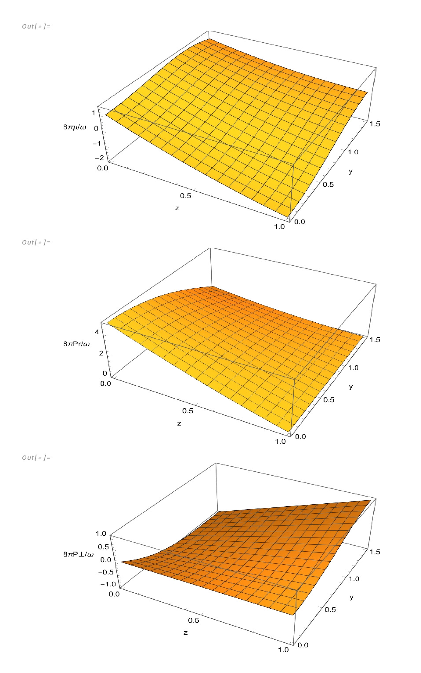
Figure 2.
as function offor the condition. Regions A and B correspond to negative and positive values ofrespectively, for solution I.
Figure 2.
as function offor the condition. Regions A and B correspond to negative and positive values ofrespectively, for solution I.
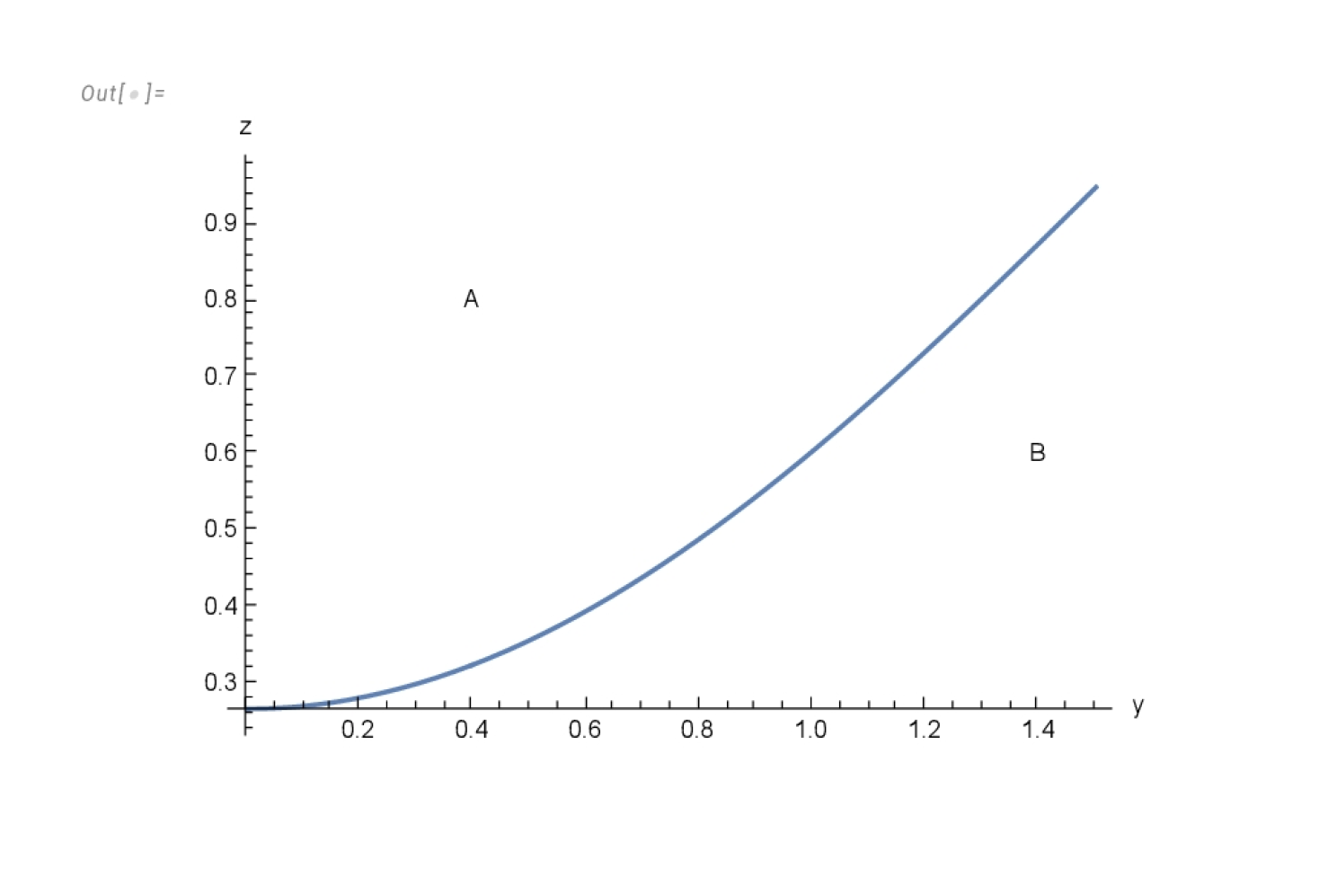
Figure 3.
, and, as functions ofandfor solution II.
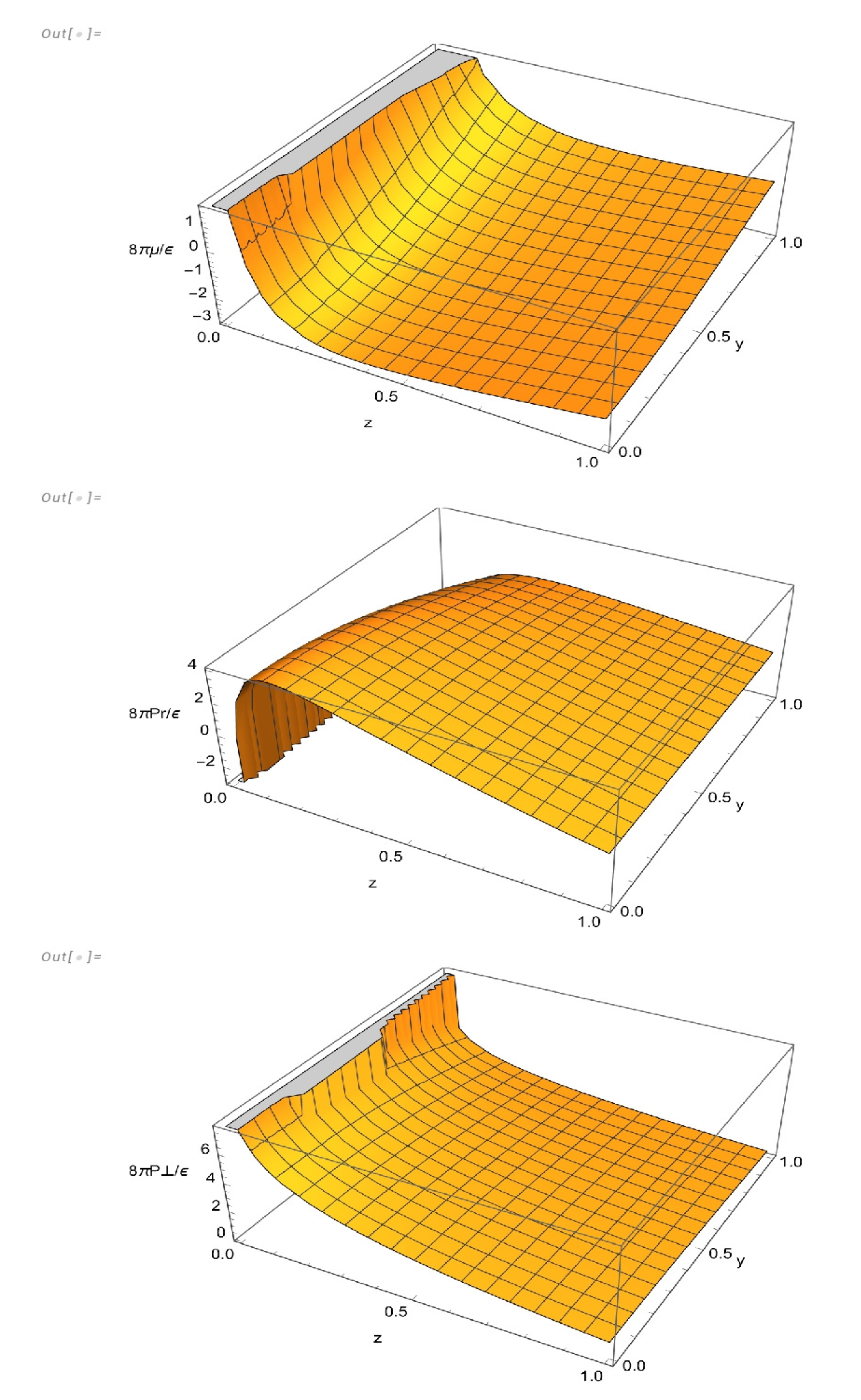
Figure 4.
as function offor the condition. Regions A and B correspond to negative and positive values ofrespectively, for solution II.
Figure 4.
as function offor the condition. Regions A and B correspond to negative and positive values ofrespectively, for solution II.
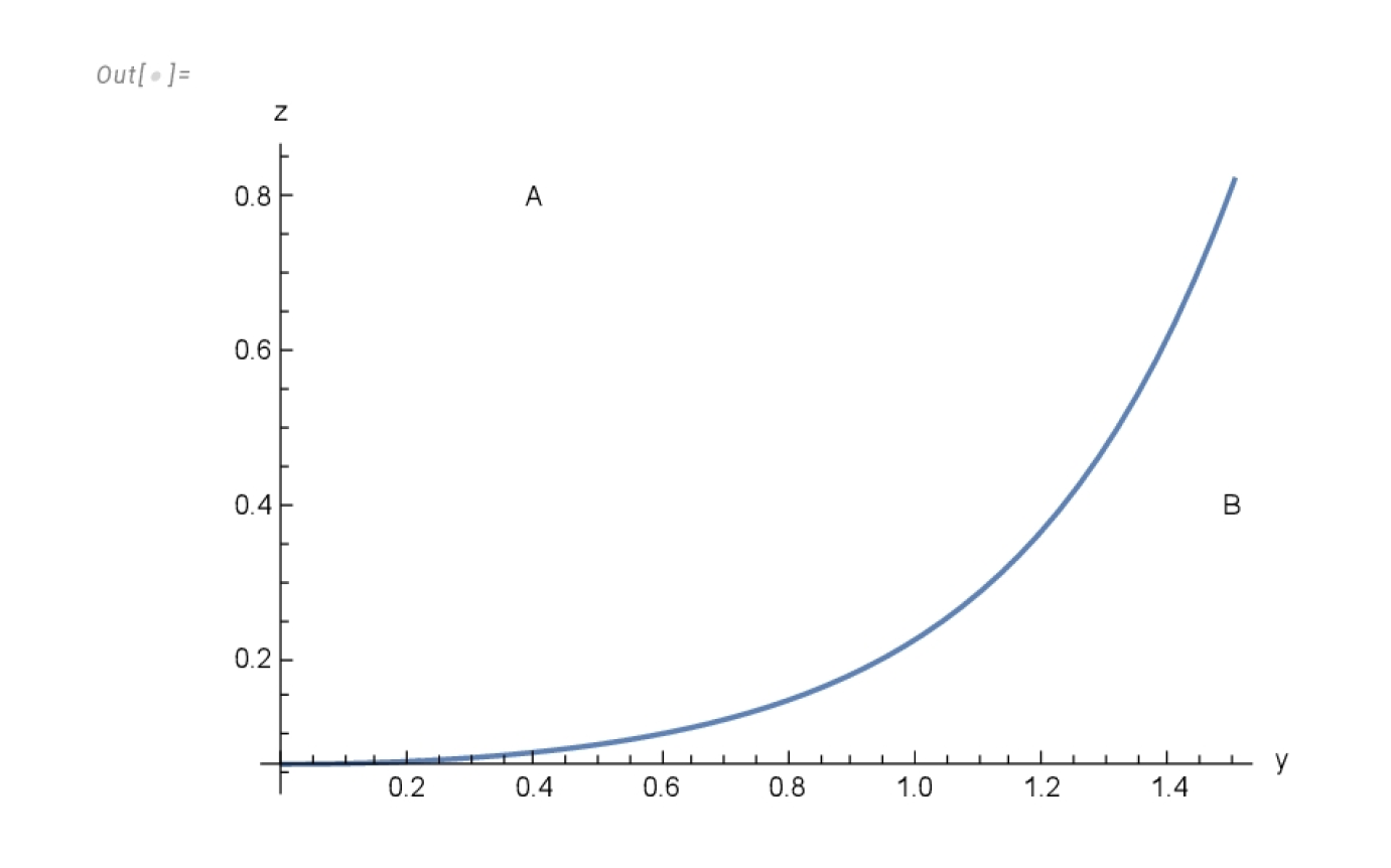
Figure 5.
, and, as functions ofandfor solution III.
Figure 6.
as function ofand; as function of; , evaluated at, as function of x, for solution III.
Figure 7.
, and, as functions ofandfor solution IV.
Figure 8.
as function ofand; as function of; , evaluated at, as function of x, for solution IV.
Disclaimer/Publisher’s Note: The statements, opinions and data contained in all publications are solely those of the individual author(s) and contributor(s) and not of MDPI and/or the editor(s). MDPI and/or the editor(s) disclaim responsibility for any injury to people or property resulting from any ideas, methods, instructions or products referred to in the content. |
© 2024 by the authors. Licensee MDPI, Basel, Switzerland. This article is an open access article distributed under the terms and conditions of the Creative Commons Attribution (CC BY) license (http://creativecommons.org/licenses/by/4.0/).
Copyright: This open access article is published under a Creative Commons CC BY 4.0 license, which permit the free download, distribution, and reuse, provided that the author and preprint are cited in any reuse.


