Submitted:
19 March 2025
Posted:
20 March 2025
You are already at the latest version
Abstract
The rapid advancement in computing power, coupled with the ability to collect vast amounts of data, has created new opportunities for industrial applications. While time-domain industrial signals typically do not allow for direct stability assessment or the detection of abnormal situations, alternative representations can reveal hidden features. This paper introduces a simple algorithm that is not directly linked to contemporary machine learning methods, designed to analyze industrial data from a standard automation system. The algorithm generates clear graphical representations to aid in controlling the production process. Specifically, we propose using time-shifted maps derived from data series collected by an acceleration sensor mounted on a robot base. Furthermore, we numerically simulated three distinct anomalous scenarios and presented their corresponding graphical representations.
Keywords:
industrial data analysis
; monitoring of industrial processes
; predictive maintenance
; production in a robotic cell
1. Introduction
The rapid development of Big Data processing technologies has revolutionized various industries by enabling the collection, storage, and analysis of vast amounts of data. This transformation is particularly evident in industrial settings, where data-driven approaches are increasingly employed to optimize processes, enhance efficiency, and ensure product quality. The integration of Artificial Intelligence (AI) and machine learning (ML) with Big Data has opened new ways for predictive analytics, anomaly detection, and process optimization, marking a shift toward smarter and more adapt-able industrial systems [1,2,3]. However, leveraging Big Data in industrial contexts is not without challenges. The complexity arises from the dynamic nature of manufacturing systems, variability in operational conditions, and the need to balance efficiency, quality, and cost [4]. Moreover, industrial data often originate from heterogeneous sources, such as sensors, logs, and machine controllers, and are characterized by high dimensionality, noise, and variability [5,6]. An essential aspect of industrial data analysis is anomaly detection, which plays a critical role in maintaining system reliability and production continuity. Various methods, including supervised and unsupervised machine learning, have been applied to detect anomalies in complex systems [7,8,9,10,11]. Despite their effectiveness, these methods often require significant computational re-sources, specialized expertise, and large labeled datasets, which can limit their accessibility for small and medium-sized enterprises (SMEs) [12,13,14]. However, this remains a complex challenge, depending on data scalability, real-time data processing, predictive analytics, the industrial sector, and data visualization [15,16,17,18,19,20,21,22,23,24,25,26,27,28,29].
In this study, we propose an approach evaluated under realistic industrial conditions. Specifically, we analyze data from an acceleration sensor mounted on the mechanical base of a robot, using Time-Shifted Mapping (TSM). This technique, often applied in deterministic chaos studies [30,31], explores relationships between position and velocity or velocity and acceleration to identify periodicities or anomalies in nonlinear physical system dynamics. Here, the TSM approach is used to detect periodicity and repeatability in the robot's operation within its cell. Additionally, by superimposing artificial perturbations on the signals, we examined the following anomalies: increasing random fluctuations, linear decay, and a rapid, temporary decrease in amplitude (a "time well"). These anomalies mimic scenarios such as increased random vibration due to loosening or broken connections in the robot cell, gradual loss of actuator movement from a power supply drop, or abrupt movement interruptions caused by mechanical or power failures. The paper provides details on the data origin, introduces the TSM approach, analyzes the data, and presents final remarks. The goal is to propose a simple, user-friendly graphical method for industrial data analysis to enhance production quality.
2. Theoretical Foundations
2.1. Deterministic Chaos as Example of Complex Behavior of Mechanical Systems
To understand more In many fields of science and technology, particularly in dynamic systems where operating parameters vary over time, it is possible to analyze a selected parameter using appropriate spectral analysis methods. Among the wide variety of signals, two extreme cases can be distinguished: signals with well-defined periodicity, for which classical Fourier analysis is highly effective, and completely aperiodic, random signals, for which wavelet analysis can be a suitable method.
The periodicity of the signal can be expressed as:
where is the time period. For signals exhibiting multiple frequencies simultaneously, (, additional secondary frequencies appear, and also the resulting complex signal spectrum can depend on the amplitude of the individual components. For example, for signals with two primary frequencies, and , the resulting signal may include frequencies corresponding to their sum and difference, i.e., and respectively. Additionally, higher-order frequency components such as , , , , and other multiples of sums and differences may also appear, though usually with vanishingly small amplitudes.
A crucial issue in industrial signals, which has practical significance, is whether periodicity is synonymous with defect occurrence. This question is directly related to the concept of deterministic chaos, i.e., the possibility of a physical system predictably transitioning into aperiodic behavior.
For dynamical systems governed by deterministic chaos, several well-established analytical methods are used, often with convenient graphical representations of system variability. These include phase diagrams, Poincaré sections, and bifurcation diagrams. In this work, we do not strictly apply deterministic chaos methods but instead focus on the analysis of two-dimensional phase diagrams applied to time-varying acceleration signals measured at selected points in a robotic cell, e.g., using a sensor attached to the base of a welding robot.
A phase diagram, in its basic form, represents the relationship between the rate of change of a time-varying signal and the signal itself, . For a perfect sinusoidal signal its first time derivative is . The phase diagram, i.e., the plot of as a function of , can form an elliptical shape (comp. Fig. 4c). In the following section, we will show that the phase diagram ( vs. ) is equivalent to the diagram ( vs. ), where is the time shift. This concept is named time-shifted mapping (TSM) of signals. By selecting an appropriate time shift, it is possible to distinguish between normal and abnormal conditions. In the actual paper, the analysis was performed using real process signals recorded from a working welding robot in a robotic cell. Failure scenarios were simulated to represent extreme conditions.
From a practical perspective in an industrial setting, real signals are often perturbed and can be represented as:
where, in general, the phase disturbance function can be periodic, aperiodic, or even random. Similarly, the signal amplitude may undergo random or, less frequently, periodic variations. For an idealized process, it can be assumed and .
In a typical industrial process, such as cyclically repeated welding in serial production, periodic variations in technological parameters naturally occur. A potential monitoring parameter, treated as a time-varying signal following the production cycle, could be the acceleration measured at various locations in the robotic cell by a point sensor.
Returning to the example of simple sinusoidal signals, and , the problem of graphical representation of periodicity reduces to finding the relation . Eliminating the explicit time dependence leads to squaring the signals and using the trigonometric identity , yielding:
Similarly, for a perturbed signal of the form , we have:
However, experimental results in the field of deterministic chaos show that the topology of phase diagrams can differ significantly from those generated by simple trigonometric functions. Analysis presented in the paper, partially overlaps with the studies of deterministic chaos, which can have practical applications in the analysis of real mechanical systems. As a concrete example of a system with more complex behavior than a simple harmonic oscillator (Eq. 3), we present phase diagrams for a driven, damped physical pendulum. This approach is discussed in detail in Baker and Golub's book [32], based on which we developed a simple numerical simulator to illustrate these results. The equation of motion for the pendulum is given by:
where is gravitation factor, is the damping factor, is the amplitude of the externally applied moment of force, which is applied periodically with the frequency , and is the moment of inertia. The equation in its normalized form () can be written as follows:
In the following we will refer to different values of the ’ amplitude (1.0, 1.07, 1.35, 1.45, 1.47, 1.50) to illustrate some results, assuming and . Thus, the behavior of the pendulum is governed by three key parameters (as a minimum of three parameters is required for chaotic behavior): the damping coefficient , the excitation frequency of the external driving force, and the amplitude of the external driving force . By selecting appropriate parameter values, different dynamic behaviors can be observed. These include cyclic motion with a single dominant frequency (Figure 1a,c)—visible in the phase diagram as a single oval, topologically similar to a perfect ellipse (Figure 1a) — as well as more complex cases, such as period-doubling bifurcations (two-cycle behavior) (Figure 1b,d), quasi-chaotic state (Figure 1e) or fully chaotic case (Figure 1f).
(Eq. 6) : single frequency case, (a), doubled frequency case, (b), single frequency case, for larger amplitude (c), doubled frequency case, (d), quasi-chaotic state, (e), fully chaotic state, (f).
The focus of this article is the presentation of such diagrams, derived from real industrial data. For visualization, we employ time-shifted diagrams, where a time-shifted signal is used to approximate the rate of change of the original signal. The key conclusion drawn from these findings is that in dynamic systems influenced by multiple factors (parameters), phase diagrams can exhibit highly complex topologies.
2.2. The Concept of Time-Shifted Mapping (TSM)
To understand more deeply the concept of time-shifted maps, let us consider two simple sinusoidal functions: single function (Figure 2a) with period, and the sum of and two-times more frequent function. In the next step, we can prepare the vs. plot, where represents the phase shift. By comparing Figure 2c-e, with phase shift of , , , respectively, we observe that for a phase shift equal to ¼ of the period, the graphical representation in the form of single oval indicates a single-period signal (Figure 2c). Similarly, for the function with double the frequency, the shift clearly reveals a single-period signal with twice the frequency (Figure 2f). Next, by applying the same approach with to the combination , we obtain a map with two loops, indicating two types of periodicities (Figure 2g). Furthermore, by superimposing random values (noise) onto the two-cycled signal, the periodicities of the pure signals can still be recognized (Figure 2f).
These simple examples provide, of course, only an approximation of industrial situations. Nevertheless, as will be shown below, analyzing time-collected acceleration data offers new insights into the nature of signals. Thus, it is easy to envision scenarios where the periodic nature of the data is either unknown or not immediately apparent, especially when the collected time series are not represented by simple trigonometric functions. As will be demonstrated below, time-shifted maps exhibit a significant resolution capability across various cases, including unpredictable and undesirable ones.
As mentioned above, in chaotic deterministic systems, analyzing the relationships between dynamical variables (e.g., generalized positions) and their velocities is a common practice [23]. The relationships can be presented as two-dimensional figures. From a numerical perspective, in the simplest case, the relationship between position at a later time and the position at an earlier time can be expressed as
where is the time-step value, and is the proportionality factor. After some straightforward derivations, it can be shown that
with a time-dependent proportionality factor , this means the velocity-position diagram (related to Eq. 7) can be used interchangeably with appropriately time-shifted position data (related Eq. 8) to obtain an adequate graphical representation of the dynamics of the system under analysis. It is worth noting that the maps can be created using different values of the time shift .
3. Experiment and Analysis of Data
The automation system developed for the experiment was divided into three interconnected layers: control, visualization with HMI (Human-Machine Interface), and SCADA (Supervisory Control and Data Acquisition). The main component of the control layer was the PLC, which managed the operation of all actuators and measuring devices, enabling the process to run in automatic mode. The Siemens S7-1500 controller used in the experiment had been programmed in the TIA Portal environment. The visualization layer consisted of a screen and touch panel integrated with an industrial PC. Visualization and control of the system were implemented using Zenon 8.2 software from COPA-DATA. This software employed a communication plug-in mechanism to connect with Siemens controllers in various ways, with a focus on the OPC-UA (Open Platform Communication - Unified Architecture) communication protocol, which was one of the most promising technologies within the Industry 4.0 framework. The SCADA system fulfilled several roles. Primarily, it acted as a central hub for data collected from the control layer. This data was analyzed for diagnostics, optimization, failure prediction, and production status reporting. The analysis results were displayed within the HMI layer. Given the cell's ability to function in both stand-alone and collaborative modes, the SCADA system had been divided into two subsystems: a local subsystem tied to the PLC and a global subsystem supporting the operation of multiple robot cells. The current experiment utilized the local subsystem.
The data were collected using an acceleration sensor (Baluff BCM0001) [33] mounted on the mechanical base of the robot (Figure 3). The Kuka KR 270 robot [34] was installed inside a fully enclosed robotic cell measuring approximately 3 m × 3 m × 3 m. The walls of the cell consisted of uniform, flat steel sheets mounted on a frame and connected to a ground frame made of T-bars, which also supported the robot base. All components of the cell enclosure were securely fastened with bolted or welded joints. This setup ensured that vibrations generated by the robot propagated throughout the structure, particularly to the robot’s base and walls of the robotic cell.
The robot performed repetitive movements related to the welding process of small metallic parts secured to a rotary table. The entire experiment lasted 2,700 seconds, with acceleration and velocity measured at 0.25-second intervals. The stored values represented the root mean square (RMS) of the peak-to-peak acceleration amplitudes. Since acceleration is proportional to the rate of change of velocity and both quantities exhibited the same frequency characteristics, the peak-to-peak acceleration amplitude was chosen for further analysis as a sufficiently representative signal. Throughout the article, acceleration values are expressed in g (Earth’s gravitational acceleration).
Figure 4 shows an example of several robotic work steps recorded by the acceleration sensor, highlighting characteristic time periods relevant to the TSM methodology. Figure 5a presents the data collected over 2,700 seconds, while Figure 5b-d illustrate numerically introduced disturbances to the original signal. These cases are analyzed in detail below. Before proceeding, we introduce the TSM concept, which involves time-shifting a data series relative to the original to generate 2D representations.
3.1. Experimental Data Analysis
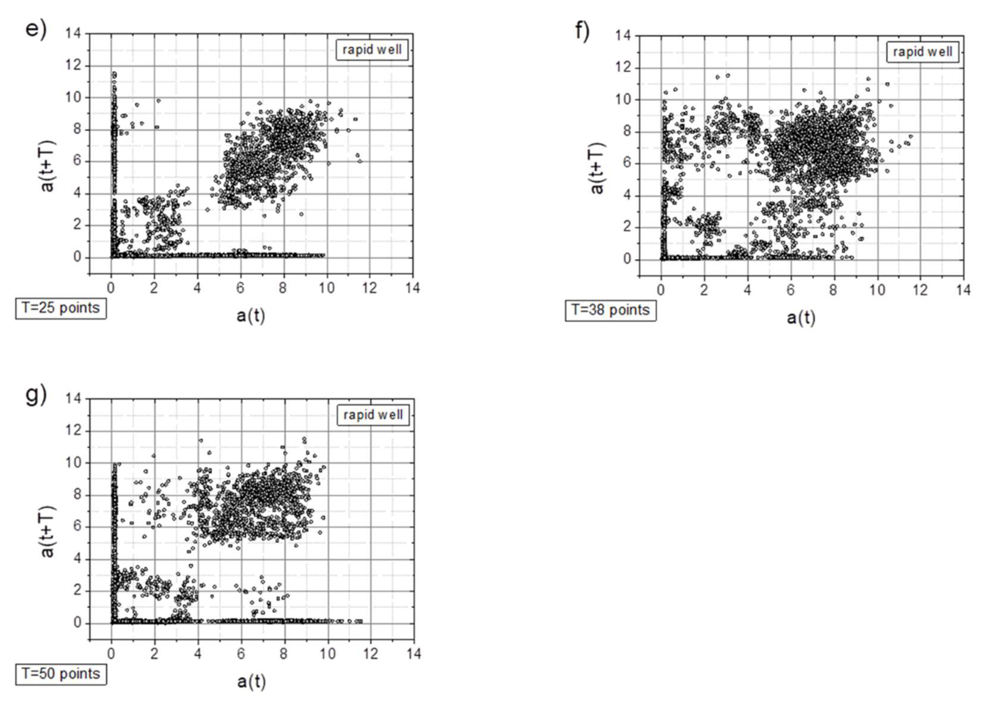
Below, we present the TSM results for the originally registered data (Figure 6), data with artificially added noise (Figure 7), data with a linear signal drop lasting from the beginning to the end of the collection period (Figure 8), and data with a rapid drop (a "well") in the signal (Figure 9). The maps were generated using different time shifts, expressed in “points” (time steps), where a single step corresponds to 0.25 s, as mentioned above. Since the periods shown in Figure 4 are 3.25 s, 6.25 s, 9.5 s, and 12.5 s, the corresponding values in “points” are 13, 25, 38, and 50, respectively. Similarly, considering the optimal choice of time shift (phase shift) as ¼ of the period, the respective values are 3, 6, 10, and 13 points. However, after evaluating various options, we present results below for time-shift values (in points) of 3, 6, 9, 12, 25, 38, and 50, as these are most useful for characterizing the data.
As can be seen from the figures above, there is an unambiguous link between the existing production situation and the spatial distribution of measurement points. These distributions can be easily classified using appropriate image analysis methods, which is beyond the scope of the current article.
4. Discussion and Conclusions
A closer look at the obtained results reveals the following observations:
- In general, all charts, except those with a time shift of T=6 points, proved to be effective for analyzing the registered signals.
- Adding a random factor to the signal disrupts its periodicity: on a map with a time shift of T=9 points (cf. Figure 7a and 7c), the map completely changes its character.
- The linear decay of the signal results in the appearance of new collinear sets of points on the chart (e.g., Figure 8c).
- Along with the observed periodicities, areas of high randomness are clearly visible—cf. maps for T=25 points, particularly for accelerations exceeding 5g (depending on the signal type).
The graphical data presentation method proposed in this paper, the approach related to deterministic chaos methods, demonstrates sensitivity to the nature of the collected data, effectively distinguishing between two dominant components: periodic and stochastic. By applying various modifications to the original signals, the TSM method has proven to be both representative and selective for the cases presented in this analysis.
A significant advantage of the two-dimensional TSM graph is its ability to allow production process supervisors to observe and draw preliminary conclusions. Furthermore, the resulting maps, which reflect modifications caused by changes in technological parameters, are highly suitable for precise and unambiguous analysis, such as employing unsupervised machine learning clustering techniques. This area of application remains underexplored and will be the focus of future research on industrial data obtained from operational robotic systems.
Author Contributions
Conceptualization, all authors; methodology, T.B.,A.D. and Sz.B.; software, T.B. and A.D.; vali-dation, T.B., J.W., S.B. and Sz.B.; formal analysis, T.B and Z.S.; investigation, T.B., S.B. and Sz.B.; resources, J.W. and Z.S.; writing—original draft preparation, T.B. and A.D.; writing—review and editing, all authors; visualization, T.B.; supervision, all authors; funding acquisition, Z.S. All authors have read and agreed to the published version of the manuscript.
Funding
This research was funded by The National Centre for Research and Development, Poland, grant “Development of energy-efficient, adaptive robotic cells with Industry 4.0 features, dedicated to the creation of a modular, freely complex and interconnected set of production machines or stand-alone operation” No. POIR.01.01.01-00-1032/19.
Institutional Review Board Statement
Not applicable.
Informed Consent Statement
Not applicable.
Data Availability Statement
The original contributions presented in the study are included in the article, further inquiries can be directed at the corresponding author.
Conflicts of Interest
The authors declare no conflicts of interest. The funders had no role in the design of the study; in the collection, analyses, or interpretation of data; in the writing of the manuscript; or in the decision to publish the results.
References
- Ding, H.; Tian, J.; Yu, W.; Wilson, D.I.; Young, B.R.; Cui, X.; Xin, X.; Wang, Z.; Li, W. The Application of Artificial Intelligence and Big Data in the Food Industry. Foods 2023, 12, 4511. [Google Scholar] [CrossRef]
- Sorger, M.; Ralph, B.J.; Hartl, K.; Woschank, M.; Stockinger, M. Big Data in the Metal Processing Value Chain: A Systematic Digitalization Approach under Special Consideration of Standardization and SMEs. Applied Sciences 2021, 11, 9021. [Google Scholar] [CrossRef]
- Kurnia Putri, R.; Athoillah, M. Artificial Intelligence and Machine Learning in Digital Transformation: Exploring the Role of AI and ML in Reshaping Businesses and Information Systems. In Advances in Digital Transformation - Rise of Ultra-Smart Fully Automated Cyberspace; IntechOpen, 2024.
- Raska, P.; Ulrych, Z.; Malaga, M. Data Reduction of Digital Twin Simulation Experiments Using Different Optimisation Methods. Applied Sciences 2021, 11, 7315. [Google Scholar] [CrossRef]
- Al-Abassi, A.; Karimipour, H.; HaddadPajouh, H.; Dehghantanha, A.; Parizi, R.M. Industrial Big Data Analytics: Challenges and Opportunities. In Handbook of Big Data Privacy; Springer International Publishing: Cham, 2020; pp. 37–61. [Google Scholar]
- Wang, J.; Zhang, W.; Shi, Y.; Duan, S.; Liu, J. Industrial Big Data Analytics: Challenges, Methodologies, and Applications. 2018.
- Panza, M.A.; Pota, M.; Esposito, M. Anomaly Detection Methods for Industrial Applications: A Comparative Study. Electronics (Basel) 2023, 12, 3971. [Google Scholar] [CrossRef]
- Grunova, D.; Bakratsi, V.; Vrochidou, E.; Papakostas, G.A. Machine Learning for Anomaly Detection in Industrial Environments. In Proceedings of the EEPES 2024; MDPI: Basel Switzerland, August 7, 2024; p. 25. [Google Scholar]
- Serradilla, O.; Zugasti, E.; Ramirez de Okariz, J.; Rodriguez, J.; Zurutuza, U. Adaptable and Explainable Predictive Maintenance: Semi-Supervised Deep Learning for Anomaly Detection and Diagnosis in Press Machine Data. Applied Sciences 2021, 11, 7376. [Google Scholar] [CrossRef]
- Mishra, A.; Dasgupta, A. Supervised and Unsupervised Machine Learning Algorithms for Forecasting the Fracture Location in Dissimilar Friction-Stir-Welded Joints. Forecasting 2022, 4, 787–797. [Google Scholar] [CrossRef]
- Wu, B.; Wang, X. Industrial Image Anomaly Detection via Self-Supervised Learning with Feature Enhancement Assistance. Applied Sciences 2024, 14, 7301. [Google Scholar] [CrossRef]
- Kannan, S.; Gambetta, N. Technology-Driven Sustainability in Small and Medium-Sized Enterprises: A Systematic Literature Review. Journal of Small Business Strategy 2025, 35. [Google Scholar] [CrossRef]
- Rupeika-Apoga, R.; Petrovska, K. Barriers to Sustainable Digital Transformation in Micro-, Small-, and Medium-Sized Enterprises. Sustainability 2022, 14, 13558. [Google Scholar] [CrossRef]
- Díaz-Arancibia, J.; Hochstetter-Diez, J.; Bustamante-Mora, A.; Sepúlveda-Cuevas, S.; Albayay, I.; Arango-López, J. Navigating Digital Transformation and Technology Adoption: A Literature Review from Small and Medium-Sized Enterprises in Developing Countries. Sustainability 2024, 16, 5946. [Google Scholar] [CrossRef]
- Theodorakopoulos, L.; Theodoropoulou, A.; Stamatiou, Y. A State-of-the-Art Review in Big Data Management Engineering: Real-Life Case Studies, Challenges, and Future Research Directions. Eng 2024, 5, 1266–1297. [Google Scholar] [CrossRef]
- Andronie, M.; Lăzăroiu, G.; Iatagan, M.; Hurloiu, I.; Ștefănescu, R.; Dijmărescu, A.; Dijmărescu, I. Big Data Management Algorithms, Deep Learning-Based Object Detection Technologies, and Geospatial Simulation and Sensor Fusion Tools in the Internet of Robotic Things. ISPRS Int J Geoinf 2023, 12, 35. [Google Scholar] [CrossRef]
- Andronie, M.; Lăzăroiu, G.; Karabolevski, O.L.; Ștefănescu, R.; Hurloiu, I.; Dijmărescu, A.; Dijmărescu, I. Remote Big Data Management Tools, Sensing and Computing Technologies, and Visual Perception and Environment Mapping Algorithms in the Internet of Robotic Things. Electronics (Basel) 2022, 12, 22. [Google Scholar] [CrossRef]
- Song, Q.; Zhao, Q. Recent Advances in Robotics and Intelligent Robots Applications. Applied Sciences 2024, 14, 4279. [Google Scholar] [CrossRef]
- Zabala-Vargas, S.; Jaimes-Quintanilla, M.; Jimenez-Barrera, M.H. Big Data, Data Science, and Artificial Intelligence for Project Management in the Architecture, Engineering, and Construction Industry: A Systematic Review. Buildings 2023, 13, 2944. [Google Scholar] [CrossRef]
- Licardo, J.T.; Domjan, M.; Orehovački, T. Intelligent Robotics—A Systematic Review of Emerging Technologies and Trends. Electronics (Basel) 2024, 13, 542. [Google Scholar] [CrossRef]
- Skėrė, S.; Žvironienė, A.; Juzėnas, K.; Petraitienė, S. Decision Support Method for Dynamic Production Planning. Machines 2022, 10, 994. [Google Scholar] [CrossRef]
- Rosin, F.; Forget, P.; Lamouri, S.; Pellerin, R. Enhancing the Decision-Making Process through Industry 4.0 Technologies. Sustainability 2022, 14, 461. [Google Scholar] [CrossRef]
- Gaworski, M.; Borowski, P.F.; Kozioł, Ł. Supporting Decision-Making in the Technical Equipment Selection Process by the Method of Contradictory Evaluations. Sustainability 2022, 14, 7911. [Google Scholar] [CrossRef]
- Liu, S.-F.; Wang, S.-Y.; Tung, H.-H. A Comprehensive Decision-Making Approach for Strategic Product Module Planning in Mass Customization. Mathematics 2024, 12, 1745. [Google Scholar] [CrossRef]
- Ulewicz, R.; Siwiec, D.; Pacana, A. A New Model of Pro-Quality Decision Making in Terms of Products’ Improvement Considering Customer Requirements. Energies (Basel) 2023, 16, 4378. [Google Scholar] [CrossRef]
- Krajčovič, M.; Bastiuchenko, V.; Furmannová, B.; Botka, M.; Komačka, D. New Approach to the Analysis of Manufacturing Processes with the Support of Data Science. Processes 2024, 12, 449. [Google Scholar] [CrossRef]
- Yang, Q.; Guo, R. An Unsupervised Method for Industrial Image Anomaly Detection with Vision Transformer-Based Autoencoder. Sensors 2024, 24, 2440. [Google Scholar] [CrossRef]
- Panza, M.A.; Pota, M.; Esposito, M. Anomaly Detection Methods for Industrial Applications: A Comparative Study. Electronics (Basel) 2023, 12, 3971. [Google Scholar] [CrossRef]
- Song, G.; Hong, S.H.; Kyzer, T.; Wang, Y. U-TFF: A U-Net-Based Anomaly Detection Framework for Robotic Manipulator Energy Consumption Auditing Using Fast Fourier Transform. Applied Sciences 2024, 14, 6202. [Google Scholar] [CrossRef]
- Dong, C. Dynamics, Periodic Orbit Analysis, and Circuit Implementation of a New Chaotic System with Hidden Attractor. Fractal and Fractional 2022, 6, 190. [Google Scholar] [CrossRef]
- Askar, S.S.; Al-Khedhairi, A. Further Discussions of the Complex Dynamics of a 2D Logistic Map: Basins of Attraction and Fractal Dimensions. Symmetry (Basel) 2020, 12, 2001. [Google Scholar] [CrossRef]
- Baker, G.L.; Gollub, J.P. Chaotic Dynamic: an Introduction. Cambridge University Press, 1996.
- BCM0001 Sensor Specification. Available online: https://www.balluff.com/en-my/products/BCM0001. (accessed on 7 January 2025).
- KR 270 R3100 Ultra K-F ROBOT. Available online: https://my.kuka.com/s/product/kr-270-r3100-ultra-kf/01t58000002hninAAA?language=pl (accessed on 7 January 2025).
Figure 1.
Phase diagrams of damped driven physical pendulum for different driving moment of force amplitude
Figure 1.
Phase diagrams of damped driven physical pendulum for different driving moment of force amplitude
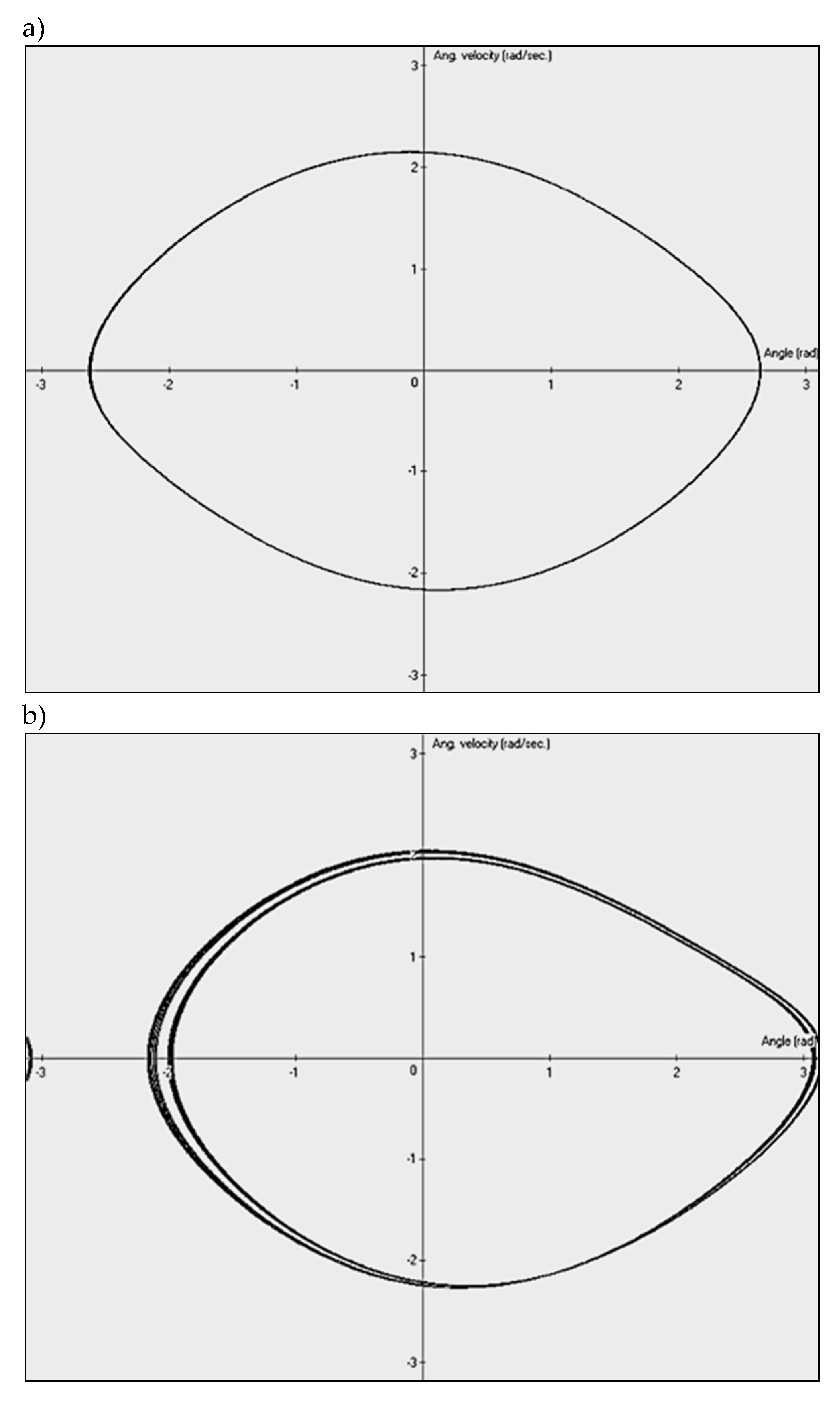
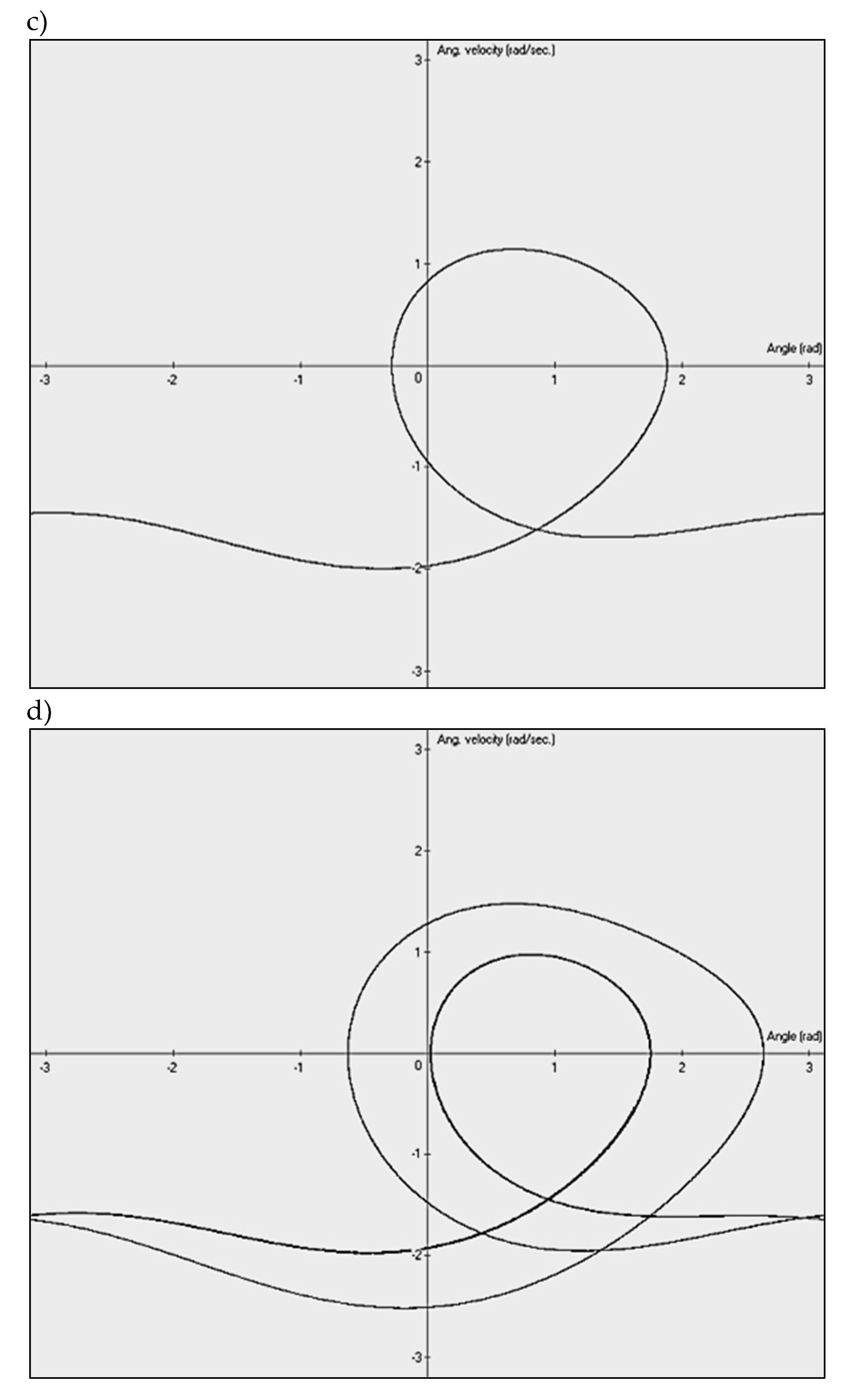

Figure 2.
The concept of time-shifted maps for examining periodicity in industrial signals. Numerical values were calculated with a resolution of 0.1 rad. (a) The basic sin(α) data series; (b) the two-times more frequent signal sin(2α); (c) the sin(α+ф) vs. sin(α) dependence with ф=0.50π rad; (d) the sin(α+ф) vs. sin(α) dependence with ф=0.25π rad; (e) the sin(α+ф) vs. sin(α) dependence with ф=2.04π rad; (f) the sin[2(α+ф)] vs. sin(2α) dependence with ф=0.25π rad; (g) the sin(2α)+sin[2(α+ф)] vs. sin(α)+sin(2α) dependence with ф=0.25π rad; and (h) the sin(2α)+sin[2(α+ф)] vs. sin(α)+sin(2α) dependence, with ф=0.25π rad along the imposed random noise.
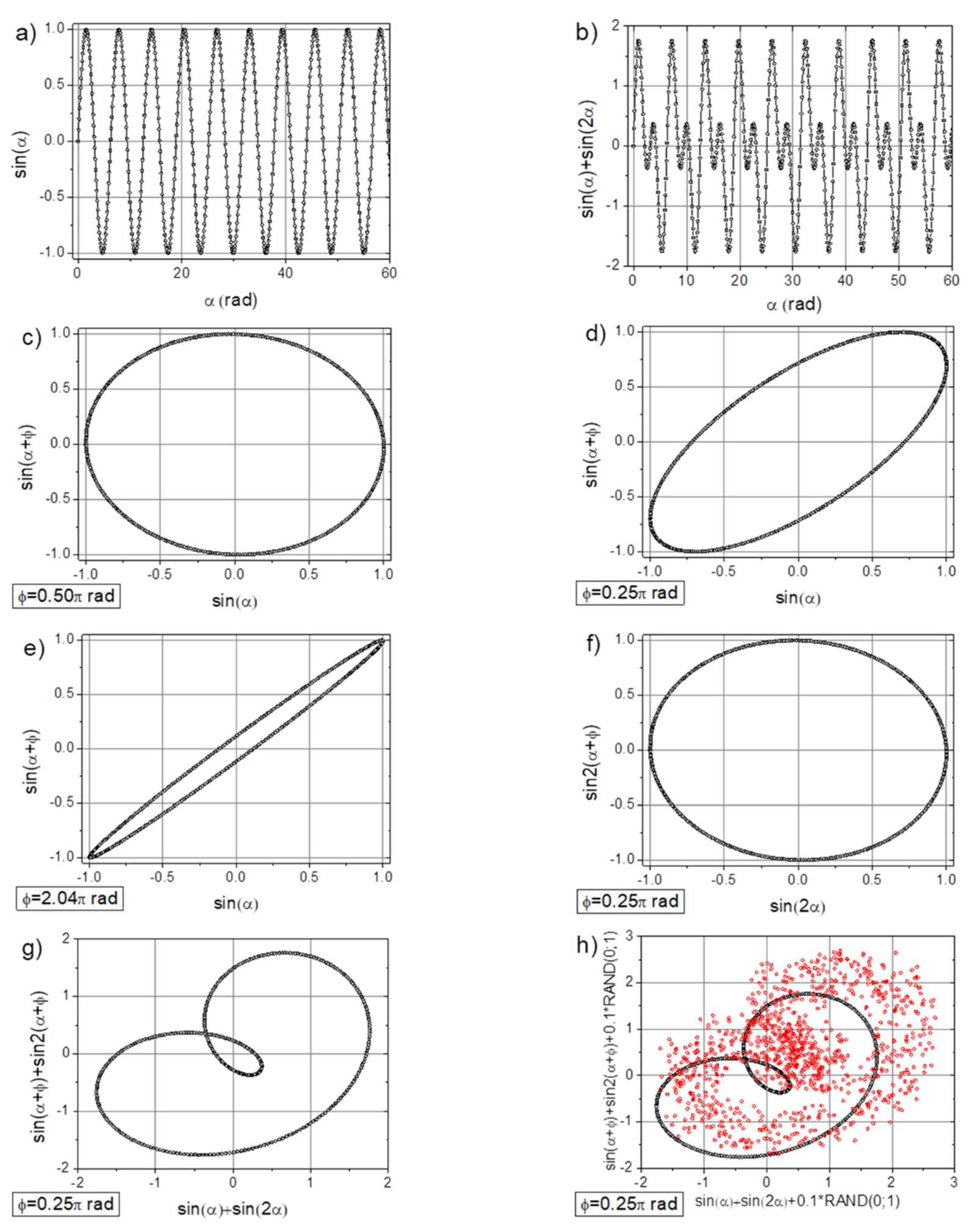
Figure 3.
An acceleration sensor (highlighted by the red oval) is mounted on the base of the robot.
Figure 4.
The registered acceleration RMS peak-to-peak magnitude values were recorded over time. The data revealed four distinct types of recognized time periodicities.
Figure 4.
The registered acceleration RMS peak-to-peak magnitude values were recorded over time. The data revealed four distinct types of recognized time periodicities.
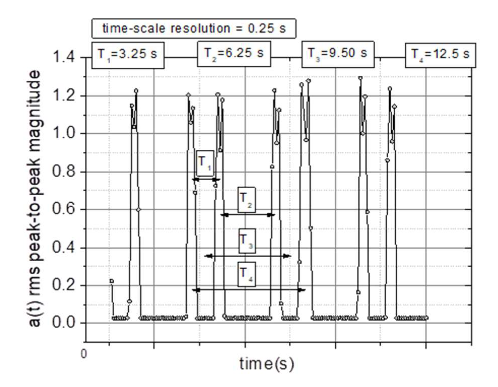
Figure 5.
Time-dependent signals from the vibration sensor (averaged acceleration peak-to-peak values): (a) original signal, (b) signal with numerical modifications to mimic potential undesired disturbances, such as random instabilities, (c) signal with a linear decline, and (d) signal showing a sudden interruption (a "well") in the working system.
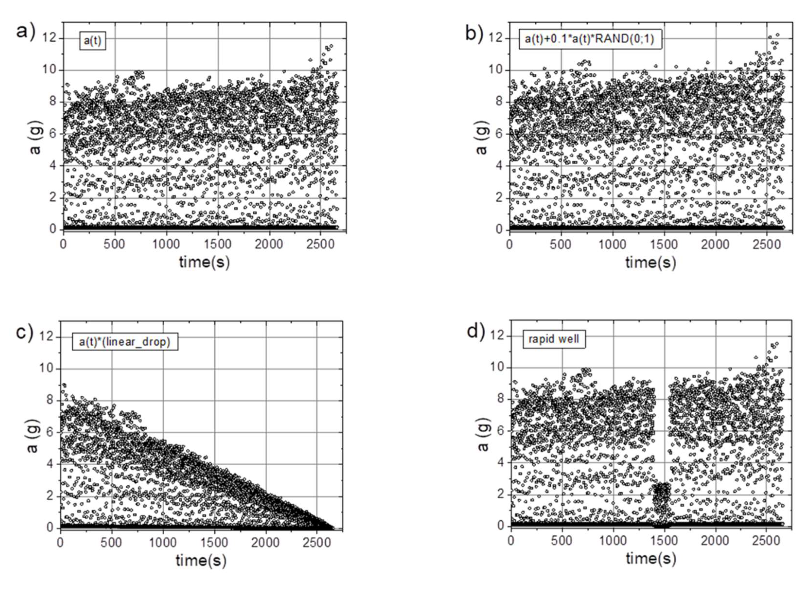
Figure 6.
The TSM results for the originally collected acceleration signal.
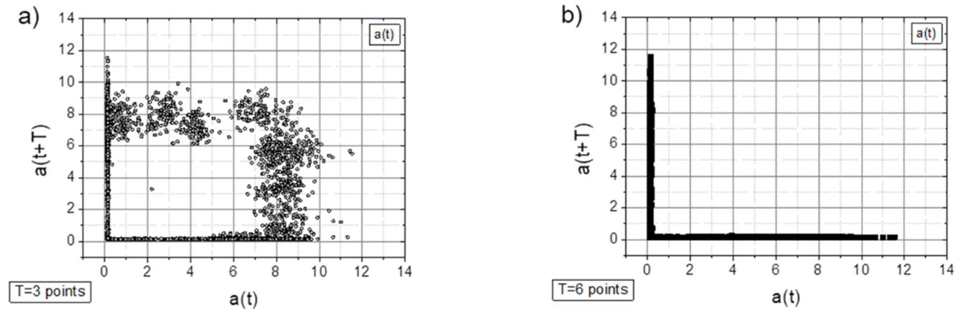
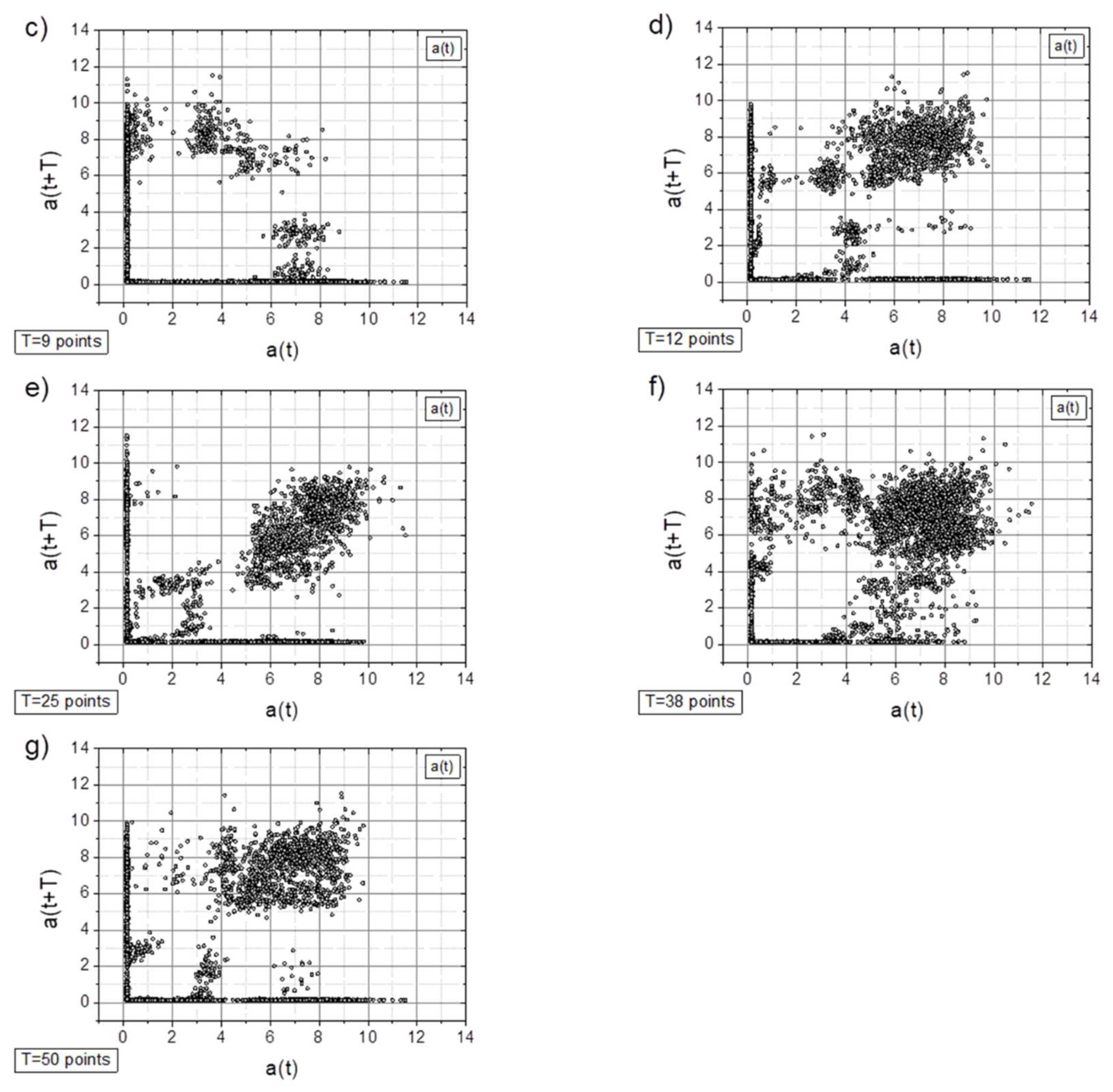
Figure 7.
The TSM results for the originally collected acceleration signal with added random values (10% of the original values multiplied by a random value taken from the [0;1] range) – cf. Figure 5b.
Figure 7.
The TSM results for the originally collected acceleration signal with added random values (10% of the original values multiplied by a random value taken from the [0;1] range) – cf. Figure 5b.
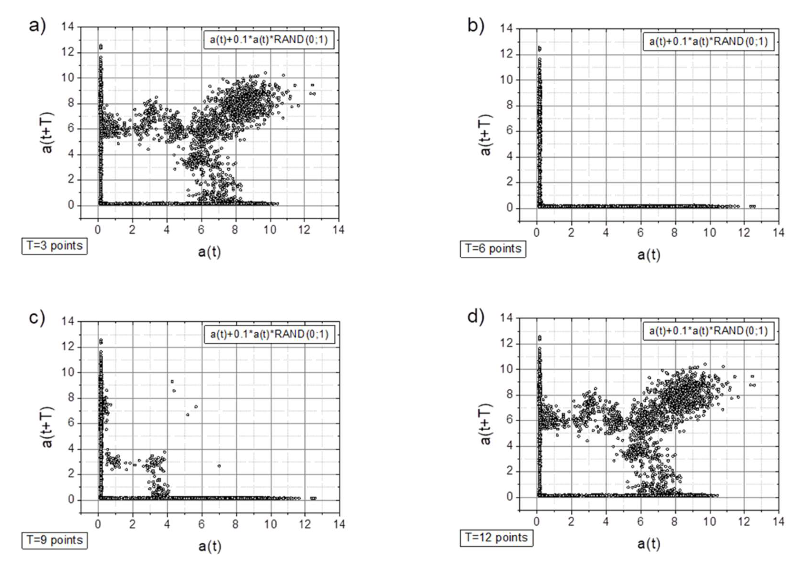
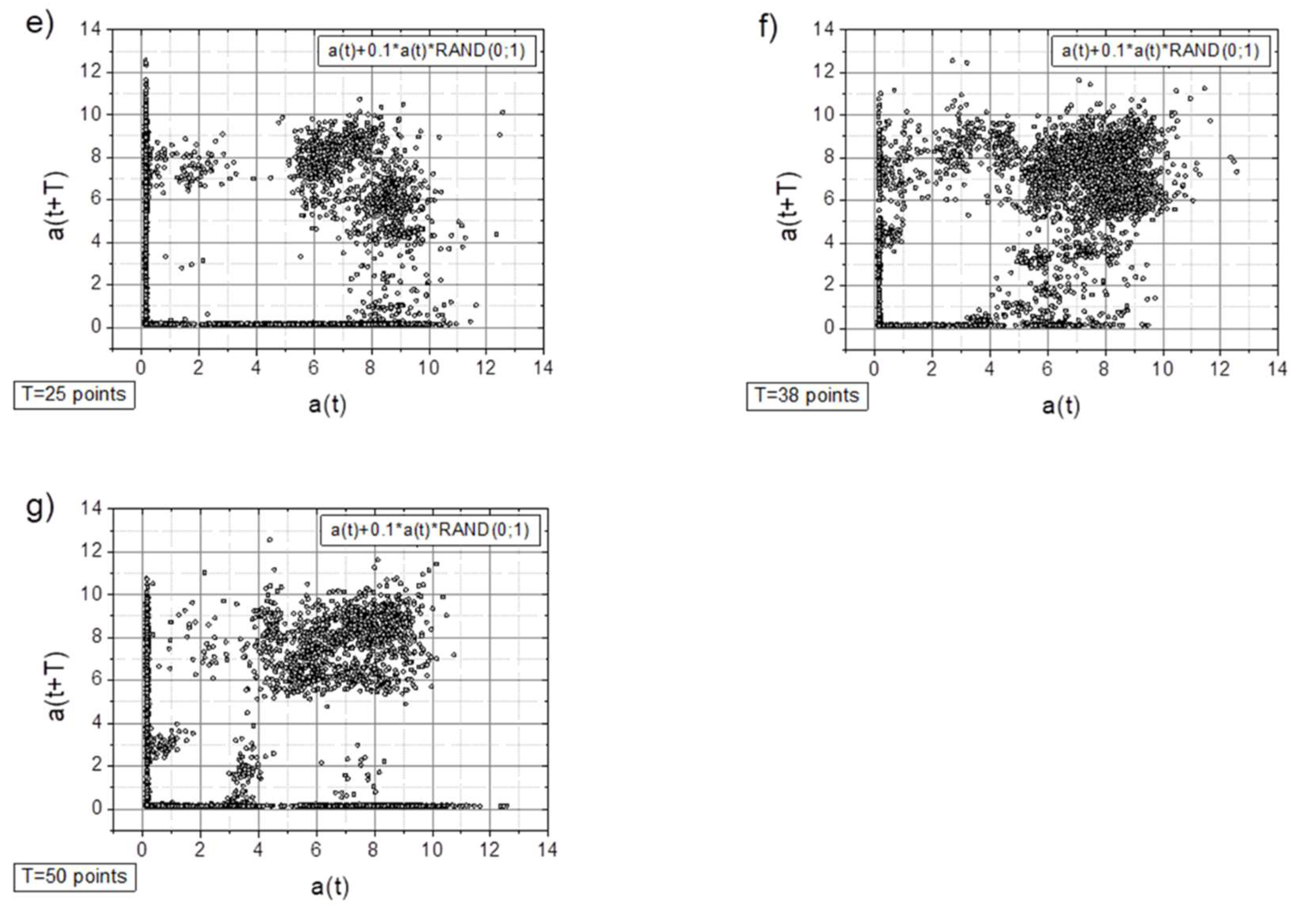
Figure 8.
The TSM results for the originally collected acceleration signal with an imposed linear drop (cf. Figure 5c).
Figure 8.
The TSM results for the originally collected acceleration signal with an imposed linear drop (cf. Figure 5c).
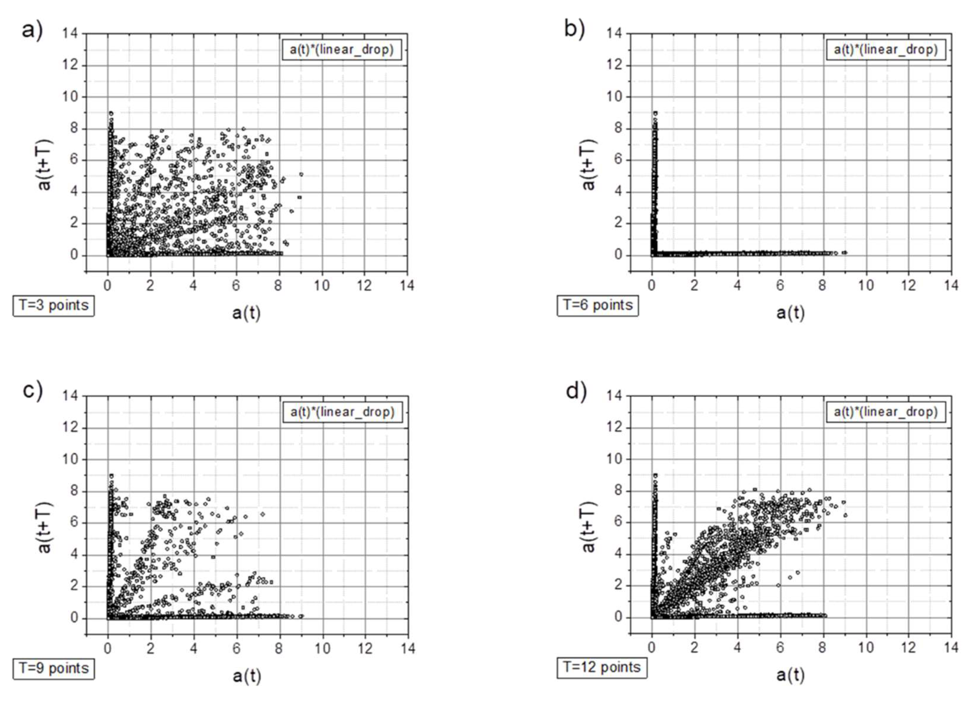
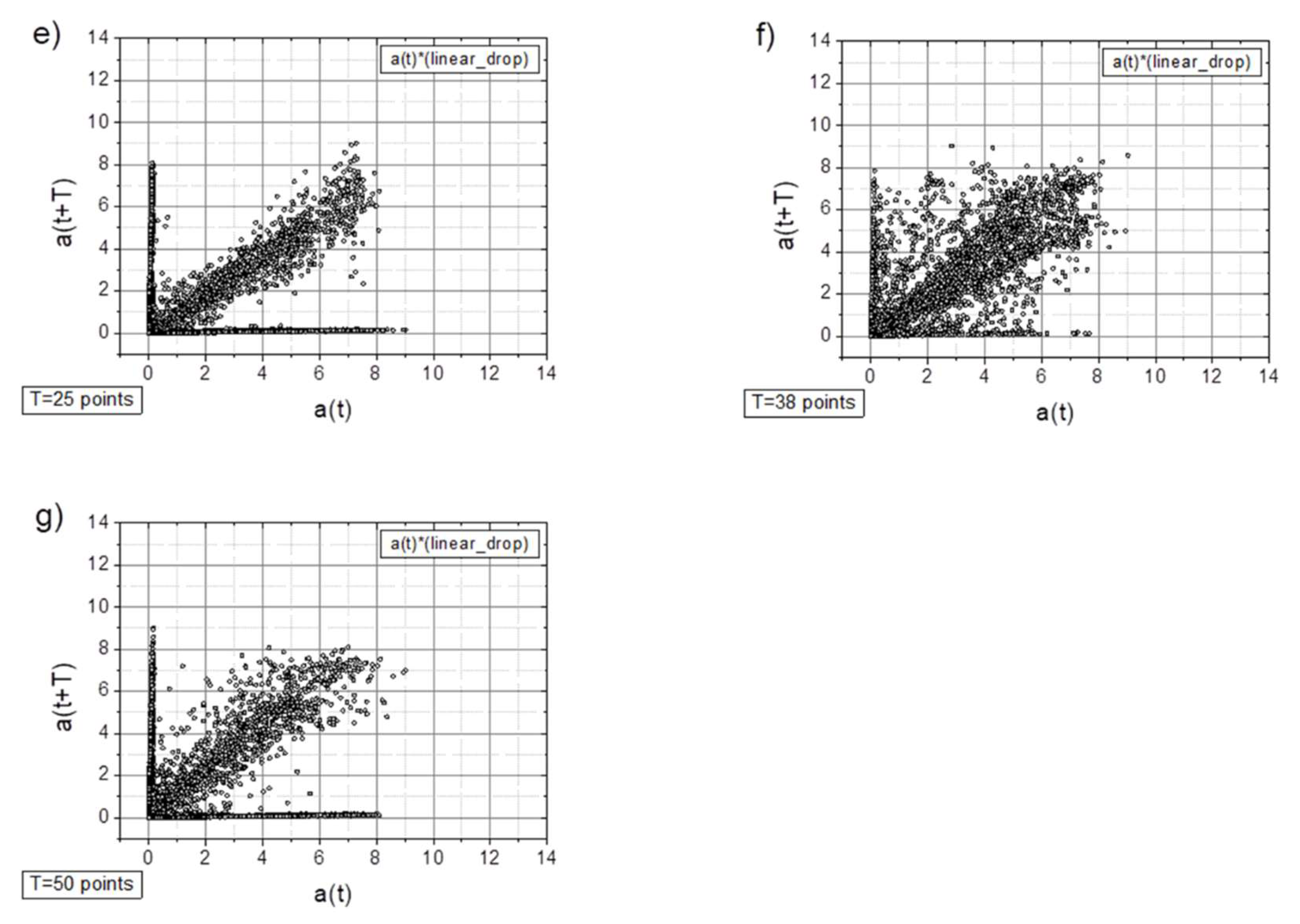
Figure 9.
The TSM results for the originally collected acceleration signal with a sudden signal break (comp. Figure 5d).
Figure 9.
The TSM results for the originally collected acceleration signal with a sudden signal break (comp. Figure 5d).

Disclaimer/Publisher’s Note: The statements, opinions and data contained in all publications are solely those of the individual author(s) and contributor(s) and not of MDPI and/or the editor(s). MDPI and/or the editor(s) disclaim responsibility for any injury to people or property resulting from any ideas, methods, instructions or products referred to in the content. |
© 2025 by the authors. Licensee MDPI, Basel, Switzerland. This article is an open access article distributed under the terms and conditions of the Creative Commons Attribution (CC BY) license (http://creativecommons.org/licenses/by/4.0/).
Copyright: This open access article is published under a Creative Commons CC BY 4.0 license, which permit the free download, distribution, and reuse, provided that the author and preprint are cited in any reuse.


