
Submitted:
29 November 2024
Posted:
29 November 2024
You are already at the latest version
Abstract
The application of modern machine learning methods in industrial conditions is a relatively new challenge and is still in the early stages of development. The currently available computing power of computers makes it possible to process a huge number of production parameters in real time. The article presents, from the practical perspective, the analysis of the manufacturing process associated with welding in a robotic cell using the unsupervised DBSCAN and specifically HDBSCAN machine learning algorithms, while showing its usefulness and advantages from the k-means algorithm. The paper also discusses the problem of predicting and monitoring undesirable situations and proposes the usage of the first derivative of the time-dependent signal of noised data to support the problem solution.
Keywords:
machine learning
; monitoring of industrial processes
; predictive maintenance
; industry 4.0
; HDBSCAN algorithm
; welding in a robotic cell
1. Introduction
The growing popularity of artificial intelligence (AI) methods, especially the methods of machine learning, found application in many branches of science and technology [1,2,3,4,5,6,7]. However, the application of machine learning methods in real industrial processes is not so widely disseminated. Many commercial devices have been equipped with controllers, like e.g. PLC (Programmable Logic Controllers) for many years, however sensorics of physical quantities in the industrial environment are underdeveloped. The main aim of this paper is to report the implementation of HDBSCAN (Hierarchical Density-Based Spatial Clustering of Applications with Noise) algorithm [8] to analyze data with the goal to anticipate undesirable situations, including those that may lead to a complete breakdown, stopping the production process, here the process based on welding technology.
The paper is organized as follows. Firstly, the real data in the time domain is presented. Next, the k-means unsupervised machine learning approach [9,10], as well as the Density Based Spatial Clustering of Application with Noise (DBSCAN) algorithm [11,12], are reviewed in order to finally justify the practical advantages of the HDBSCAN implementation [13,14]. The algorithms were tested for their effectiveness in determining the two distinct situations, namely; the well working system and, on the contrary, the system revealing some instabilities during welding. In addition, the visual information was evaluated from a practical perspective, specifically in terms of what type of graphics is better perceived by the operator who oversees the production process. Numerical analysis was performed with the use of Scikit-learn Python package [15].
Major industry players are capable of measuring many parameters in real-time, generating large amounts of data (the so-called big data), however their processing to solve practical problems is not so frequently met. Among dominating applications, we can mention geoscience [16,17,18], monitoring of transport in urban areas [19,20,21,22,23], and numerical data evaluation in data-base applications [24,25,26]. From the machine industry standpoint of view, we can meet some process optimization approaches with the use of k-means algorithm [27], including anomaly detection in automotive industry [28]. Also, the HDBSCAN method was implemented in hydropower unit monitoring [29]. Fault detection was reported in few works, for example in [30,31], while the good review of the Industry 4.0 approach, which relies on big data collection, can be found in [32].
2. Collecting Industrial Data and Samples
The subject of the presented analysis is related to data obtained during the real welding process, in a robotic cell, using a Fronius® welding system. The data were recorded over a period of 78 minutes, during which the robot cyclically repeated several types of welds, which differed in length and the shape of its welding path. Data storing has been realized at the constant rate of 4.2 seconds. During operation, the following parameters were recorded: electric current intensity (A), electric power (W), electric voltage of the welding system power supply (V), welding time (s), wire feed speed (WFS) (m/min), and the system energy consumption (kJ). The applied welding method was the MIG/MAG (the gas metal arc welding). As samples for experiments the heat exchangers suitable for domestic applications, made of ordinary carbon steel, were used (Figure 1). The typical length of the weld paths ranged from about 60 mm to 80 mm, namely there were six welds mounting the tubes around their circumferences and the eight straight welds mounting the front squared surfaces. A typical weld process, for these paths, were splitted into single events of different time duration, while a single event was no longer than 6 s.
3. Analysis of Results
The collected industrial signals are presented below in time domain (Figure 2). As can be seen, the recorded data are grouped into dominant areas, while some abnormal data, that can potentially be treated as undesirable ones, appear outside the dominant regions. For example, in Figure 1a there are five dominating areas (islands) of data, shown in detail in zoomed Figure 1b. Also, in the figure, there are two significant regions; around initial moment of registration (Time=0) – there are non-zero values of current, and zero-valued currents below the islands, registered for Time >70000. Hence, the other points reveal random behavior (abnormal data).
A more in-depth look at the behavior of the measured parameters can give a study with the omission of the time domain, which, as is widely known, is a typical preliminary step for data clustering analysis. These modified results are given in Figure 3. It is obvious that other combinations of data sets are also possible, however the relations provided are sufficiently representative for further analysis. Nevertheless, the data presented in this way does not provide the full picture, that is, the possibility to deeply recognize faults and realize the eventual corrections of the technological process.
In the following analysis, we will discuss in detail the relationship seen in Figure 3a, that is, the dependence of energy on current.
3.1. K-Means Algorithm
The classical k-means data clustering method consists of dividing data into sub-areas, for which a specific number of clusters, along with attraction centers, are determined, so that the sum of distances of individual points, measured from the cluster centers, are at minimum. In the method, the number of centers and the method of counting distances should be specified by a user. There are several possibilities. For the presented data analysis, the Euclidean quadratic distance between the actual (i-th) measured-point position and the center of the k-th cluster was used. It can be defined as
and the sum of distances, within a given cluster, and for all k-clusters, falls to a minimum
An equivalent example of the k-means clustered relationship between normalized data of energy and current, is shown in Figure 4 (on the left). Normalization is not necessary, although it is a common approach, especially met in the analysis of data belonging to completely unrelated subject areas. In the right panel of Figure 4 we justify why the existence of 4 clusters was assumed. In order to do so, we applied the so-called overall Silhouette value (SV) parameter, which states how well the data were separated to form clusters. Thus, by looking for a minimum for each i-th data point, taken from an overall N points data set, we have the following individual Silhouette values
where is the averaged distance of a given data point (i) to all N points, that is including other cluster members, and is the averaged distance between i-th point and the other points within the k-th cluster. Thus, for the N data points the overall SV parameter equals
In the presented analysis we usually looked after the first minimum in the dependence between the overall SV and the assumed number of clusters.
The optimized number of clusters has straightforward interpretation, in the case of our data, if to analyze results from the perspective of different welding times (Figure 5). Obtained clusters clearly indicate a clear relationship between the consumed energy, applied currents, and the duration of the welding process.
While the k-means analysis provides sharp boundaries between obtained areas (Figure 4) - which can be seen as an advantage of the method - then this type of graphical presentation does not deliver sufficient and fast information about undesirable situations to the operator. From the practical point of view, however, observation of the cluster-centers positions can provide some hints to the production process quality. On the other hand, such observations might not be fully objective, relying on human recognition and decisions.
3.2. DBSCAN Algorithm
In the next step forward, testing first of all, the effectiveness of monitoring the production process, we used algorithm which tried to exclude some outstanding results from clusters, the results treated as undesirable noise indicating onto non-demanding situations. The DBSCAN approach is an example of such a solution. The algorithm gives an opportunity to declare a minimum number of data points - for the assumed distance of attraction (impact range - epsylon) - in order to classify its coordinates as belonging to a given clustered region. Figure 6 shows four cases, for the assumed minimum number cluster members equal to: 5, 10, 25, and 50, again based on the same exemplary energy-current data series, in order to determine the optimum value of the impact range (epsylon range). In this way we are able to predict the expected number of clusters as well as possible number of noise points.
Comparing the previous k-means analysis, we can conclude that epsylon=10 along with minimum number of samples creating a cluster between 25 and 50 (lower panels in Figure 6) are good choices. Too small value of this parameter generates numerical instabilities, while too large one limits the number of clusters, i.e. loses information. Proper selection of these two parameters (epsylon, minimum number of points) determines the unambiguous distinction between desired data and noise, and consequently the possibility to control the stability of production process. In Figure 7 the clusterization of data is shown for different epsylon values (eps=5, 10, 15, 25) and for the same minimum number of cluster-members equal to 50.
Obtained results (comp. Figure 4 with Figure 7), especially for eps=10, identify very well, reasonably, the relevant areas of the device's operation from the point of view of the welding process. While DBSCAN algorithm has this basic advantage, the possibility to recognize outstanding data from the dominating ones, the very similar method, the HDBSCAM approach, is capable of identifying the variable density of local clusters. The variable density means the possibility to inform operator about overlapping, repeated points. This improved method will be discussed below.
3.3. HDBSCAN Algorithm
Identification the variable density of cluster members can be graphically presented as e.g. circles of variable diameter being proportional to number of samples possessing the same coordinates. The algorithm, similarly, to DBSCAN, assumes the measure of separation from one cluster to another. This measure is named cut distance, equivalent to the epsylon parameter of the DBSCAN approach. Also, in the HDBSCAN method the minimum number of data points, forming the nucleus of cluster, is the adjustable parameter. In Figure 8 several cases of the minimum data points, 15, 20, 25, 30, 40, and 80, are given (from left to right, and up to down). The cut distance has been fixed to 0.1 for further analysis.
The choice of 30 minimum samples gives an opportunity to recognize the two clusters at zero-valued current, what might be significant information about the resting mode of operation. Hence, the other relationships, between different data series, are shown in Figure 9. The data points of enhanced density are represented by larger circles, while there are no significant differences between their sizes, what means density of overlapping data points is, more or less, uniform within the process of welding.
While the HDBSCAN information is more accurate, in comparison to previously described methods, the practical observation of variable production process, thus, the observation of the above graphics is not unambiguous until the end. This is why other characteristics have been proposed. There are – registered in time – the variable number of clusters and the variable number of noised points (Figure 10). The figures given were obtained for the minimum number of samples to create a cluster equal to 30. In the figure it is easy to recognize the initial phase, after which the first two clusters have been created and, at the same time, the number of noise points have dropped down. After that moment, the production process evolved into 4-clusters state, while the number of noised point grown linearly possessing a relatively small slope (the growth rate) equal to about 0.015 points/time_step – excluding the almost final step of production, in where sudden increase in the level of noise was registered.
In order to simulate a hypothetically more inappropriate production situation, using the same kind of graphical representation, we reduced the number of samples needed to form a cluster to the value of 15. The results are shown in Figure 11.
We can therefore conclude, the number of clusters and the number of noise points reveal instabilities, e.g. for time moment equal to about 600. Another instability is seen for 660 value, when the system rapidly evolved from 4 to 6 clusters via intermediate 5-clusters state. This case is more clearly seen in the noise data figure (right panel of Figure 11), and the noise signal changes in a non-linear manner in comparison to results given in Figure 10. However, it can be said that from a practical point of view, the welded parts had no shortcomings. Consideration of the case shown in Figure 11 is only a simulation of a hypothetical, undesirable situation. Thus, returning to the main assumptions of the analyzed results, that is, the case when the minimum number of points forming a cluster is 30, in the next figure (Figure 12) we show the real-time recorded noise dependencies for other data series. The conclusion drawn from these observations is that one should not be limited to observing only one set of data. For example, for the energy-power relationship, some instabilities in the welding process are observed around Time=600, which are not visible for other sets of data series.
In order to provide even more detailed insight into the observed effect, is the usage of the 1st derivate from noise signal. These results are presented in Figure 13.
From that perspective, the two dominating, significant instabilities were detected; the first one around time-moment of 620 (seen clearly at Figure 13b) and the second situation nearly close to the production process, for time-moments above 1000 (most visible at Figure 13a,b). These two uncertain situations can be recognized in direct dependencies analysis, especially in the energy vs. power dependencies (Figure 14 and Figure 15). Both figures show the states before the abrupt change in the noise level (on the left) and during the increased level of noise (on the right).
In both cases, the registered noise level jumps reflect the system's scattered energy consumption values (0-15 kJ), for the power falls in a fuzzy range around the 3500 W value. Thus, the data has not been classified as members of clusters.
4. Discussion and Conclusions
In the paper we showed the practical implementation of unsupervised machine learning methods in the welding process of heat-exchanger samples. We provided the adequate graphical representation of production process for HDBSCAN algorithm along with comparison of its usefulness, from the perspective of the classical k-means and DBSCAN approaches, in order to classify uncertain production moments. By the use of the proposed first derivative of the registered in-time noise signal, it was possible to recognize instability in energy and power supply. Hence, the visual information, in the form of number clusters and noise level, was evaluated from a practical point of view, namely from the perspective of the technological operator who oversees the production process. We can indicate that such graphical characteristics should be observed for a few selected combinations of data series. In future work we will focus on the implementation of supervised methods, in where labeling of data is the next challenging task, especially for multidimensional results.
Author Contributions
Conceptualization, T.B. J.W. and Z.S.; methodology, T.B. and M.B.; software, T.B. and M.B.; validation, T.B and J.W.; formal analysis, T.B and Z.S..; investigation, T.B. and M.B.; resources, J.W. and Z.S.; writing—original draft preparation, T.B.; writing—review and editing, all authors; visualization, T.B.; supervision, all authors; funding acquisition, Z.S. All authors have read and agreed to the published version of the manuscript.
Funding
This research was funded by The National Centre for Research and Development, Poland, grant “Development of energy-efficient, adaptive robotic cells with Industry 4.0 features, dedicated to the creation of a modular, freely complex and interconnected set of production machines or stand-alone operation”No. POIR.01.01.01-00-1032/19.
Institutional Review Board Statement
Not applicable.
Informed Consent Statement
Not applicable.
Data Availability Statement
The original contributions presented in the study are included in the article, further inquiries can be directed at the corresponding author.
Conflicts of Interest
The authors declare no conflicts of interest. The funders had no role in the design of the study; in the collection, analyses, or interpretation of data; in the writing of the manuscript; or in the decision to publish the results.
References
- Shalev-Shwartz, S.; Ben-David, S. Understanding Machine Learning: From Theory to Algorithms; Cambridge University Press, 2014.
- Goodfellow, I.; Bengio, Y.; Courville, A. Deep Learning; MIT Press, 2016.
- Aggarwal, C. C.; Reddy, C. K. (Eds.). Data Clustering: Algorithms and Applications; CRC Press, 2013.
- Azzalini, A., & Torelli, N. (2007). Clustering via nonparametric density estimation. Statistics and Computing, 17(1), 71–80. [CrossRef]
- Kriegel, H. P., Kröger, P., Sander, J., & Zimek, A. (2009). Density-based clustering. Wiley Interdisciplinary Reviews: Data Mining and Knowledge Discovery, 1(3), 231–240.
- Campello, R. J. G. B., Hruschka, E. R., & Sander, J. (2015). Clustering based on density measures and automated cluster extraction. Data Mining and Knowledge Discovery, 29(3), 802–830.
- Campello, R. J., Moulavi, D., Zimek, A., & Sander, J. (2013). Density-based clustering based on hierarchical density estimates. In Pacific-Asia Conference on Knowledge Discovery and Data Mining (pp. 160–172). Springer.
- McInnes, L., Healy, J., & Astels, S. (2017). HDBSCAN: Hierarchical density-based clustering. Journal of Open Source Software, 2(11), 205. [CrossRef]
- Hartigan, J. A., & Wong, M. A. (1979). A K-means clustering algorithm. Applied Statistics, 28(1), 100–108.
- Jain, A. K. Data clustering: 50 years beyond K-means. Patt. Recogn. Lett. 2010, 31, 651–666. [CrossRef]
- Schubert, E., Sander, J., Ester, M., Kriegel, H. P., & Xu, X. (2017). DBSCAN revisited, revisited: Why and how you should (still) use DBSCAN. ACM Transactions on Database Systems, 42(3), 19.
- Retiti Diop Emane, C.; Song, S.; Lee, H.; Choi, D.; Lim, J.; Bok, K.; Yoo, J. Anomaly Detection Based on GCNs and DBSCAN in a Large-Scale Graph. Electronics 2024, 13, 2625. [CrossRef]
- Emmons, S., Kobourov, S., Gallant, M., & Börner, K. (2016). Analysis of network clustering algorithms and cluster quality metrics at scale. PLOS ONE, 11(7), e0159161. [CrossRef]
- Xu, R., & Wunsch, D. (2005). Survey of clustering algorithms. IEEE Transactions on Neural Networks, 16(3), 645–678.
- https://scikit-learn.org/.
- Ackermann, M. R., Blömer, J., & Sohler, C. (2010). Clustering for metric and non-metric distance measures. ACM Transactions on Algorithms, 6(4), 1–26.
- Schubert, E., Sander, J., Ester, M., Kriegel, H. P., & Xu, X. (2017). DBSCAN revisited, revisited: Why and how you should (still) use DBSCAN. ACM Transactions on Database Systems, 42(3), 19.
- Hasan, M.M.U.; Hasan, T.; Shahidi, R.; James, L.; Peters, D.; Gosine, R. Lithofacies Identification from Wire-Line Logs Using an Unsupervised Data Clustering Algorithm. Energies 2023, 16, 8116. [CrossRef]
- Han, X.; Armenakis, C.; Jadidi, M. Modeling Vessel Behaviours by Clustering AIS Data Using Optimized DBSCAN. Sustainability 2021, 13, 8162. [CrossRef]
- Munguía Mondragón, J.C.; Rendón Lara, E.; Alejo Eleuterio, R.; Granda Gutirrez, E.E.; Del Razo López, F. Density-Based Clustering to Deal with Highly Imbalanced Data in Multi-Class Problems. Mathematics 2023, 11, 4008. [CrossRef]
- Yun, K.; Yun, H.; Lee, S.; Oh, J.; Kim, M.; Lim, M.; Lee, J.; Kim, C.; Seo, J.; Choi, J. A Study on Machine Learning-Enhanced Roadside Unit-Based Detection of Abnormal Driving in Autonomous Vehicles. Electronics 2024, 13, 288. [CrossRef]
- DeMedeiros, K.; Koh, C.Y.; Hendawi, A. Clustering on the Chicago Array of Things: Spotting Anomalies in the Internet of Things Records. Future Internet 2024, 16, 28. [CrossRef]
- edersen, K.; Jensen, R.R.; Hall, L.K.; Cutler, M.C.; Transtrum, M.K.; Gee, K.L.; Lympany, S.V. K-Means Clustering of 51 Geospatial Layers Identified for Use in Continental-Scale Modeling of Outdoor Acoustic Environments. Appl. Sci. 2023, 13, 8123. [CrossRef]
- Cesario, E.; Lindia, P.; Vinci, A. Detecting Multi-Density Urban Hotspots in a Smart City: Approaches, Challenges and Applications. Big Data Cogn. Comput. 2023, 7, 29. [CrossRef]
- Gadal, S.; Mokhtar, R.; Abdelhaq, M.; Alsaqour, R.; Ali, E.S.; Saeed, R. Machine Learning-Based Anomaly Detection Using K-Mean Array and Sequential Minimal Optimization. Electronics 2022, 11, 2158. [CrossRef]
- Guerreiro, M.T.; Guerreiro, E.M.A.; Barchi, T.M.; Biluca, J.; Alves, T.A.; de Souza Tadano, Y.; Trojan, F.; Siqueira, H.V. Anomaly Detection in Automotive Industry Using Clustering Methods—A Case Study. Appl. Sci. 2021, 11, 9868. [CrossRef]
- Choi, W.-H.; Kim, J. Unsupervised Learning Approach for Anomaly Detection in Industrial Control Systems. Appl. Syst. Innov. 2024, 7, 18. [CrossRef]
- Barrera, J.M., Reina, A., Mate, A. et al. Fault detection and diagnosis for industrial processes based on clustering and autoencoders: a case of gas turbines. Int. J. Mach. Learn. & Cyber. 13, 3113–3129 (2022). [CrossRef]
- Nelson, W.; Culp, C. Machine Learning Methods for Automated Fault Detection and Diagnostics in Building Systems—A Review. Energies 2022, 15, 5534. [CrossRef]
- Vijayan, D.; Aziz, I. Adaptive Hierarchical Density-Based Spatial Clustering Algorithm for Streaming Applications. Telecom 2023, 4, 1-14. [CrossRef]
- Mazzei, D.; Ramjattan, R. Machine Learning for Industry 4.0: A Systematic Review Using Deep Learning-Based Topic Modelling. Sensors 2022, 22, 8641. [CrossRef]
- Zhang, F.; Guo, J.; Yuan, F.; Qiu, Y.; Wang, P.; Cheng, F.; Gu, Y. Enhancement Methods of Hydropower Unit Monitoring Data Quality Based on the Hierarchical Density-Based Spatial Clustering of Applications with a Noise–Wasserstein Slim Generative Adversarial Imputation Network with a Gradient Penalty. Sensors 2024, 24, 118. [CrossRef]
Figure 1.
The heat exchanger used in the industrial experiment. The total length of the sample equals 385 mm, while its main squared cross section is 60 mm x 60 mm.
Figure 1.
The heat exchanger used in the industrial experiment. The total length of the sample equals 385 mm, while its main squared cross section is 60 mm x 60 mm.
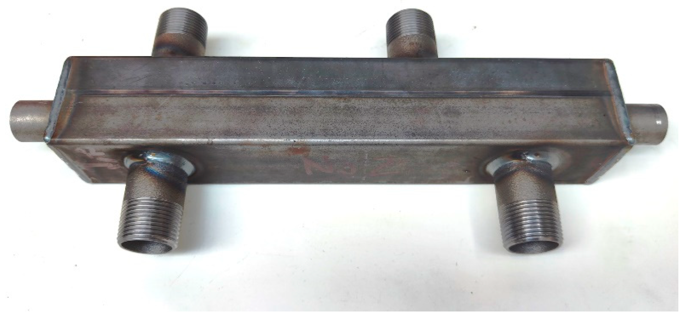
Figure 2.
The registered data in time-domain: current (a), current with initial phase excluded (b), power (c), voltage (d), welding time (e), and the wire feed speed (WFS) (f).
Figure 2.
The registered data in time-domain: current (a), current with initial phase excluded (b), power (c), voltage (d), welding time (e), and the wire feed speed (WFS) (f).
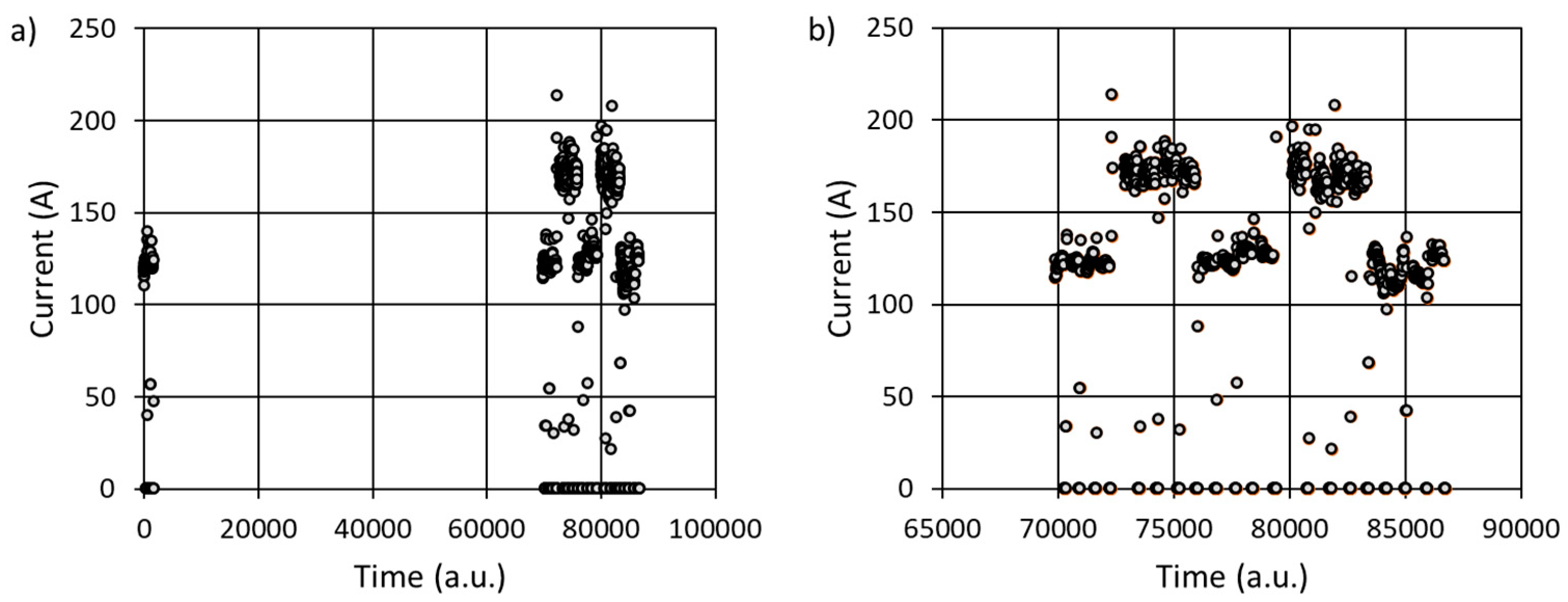
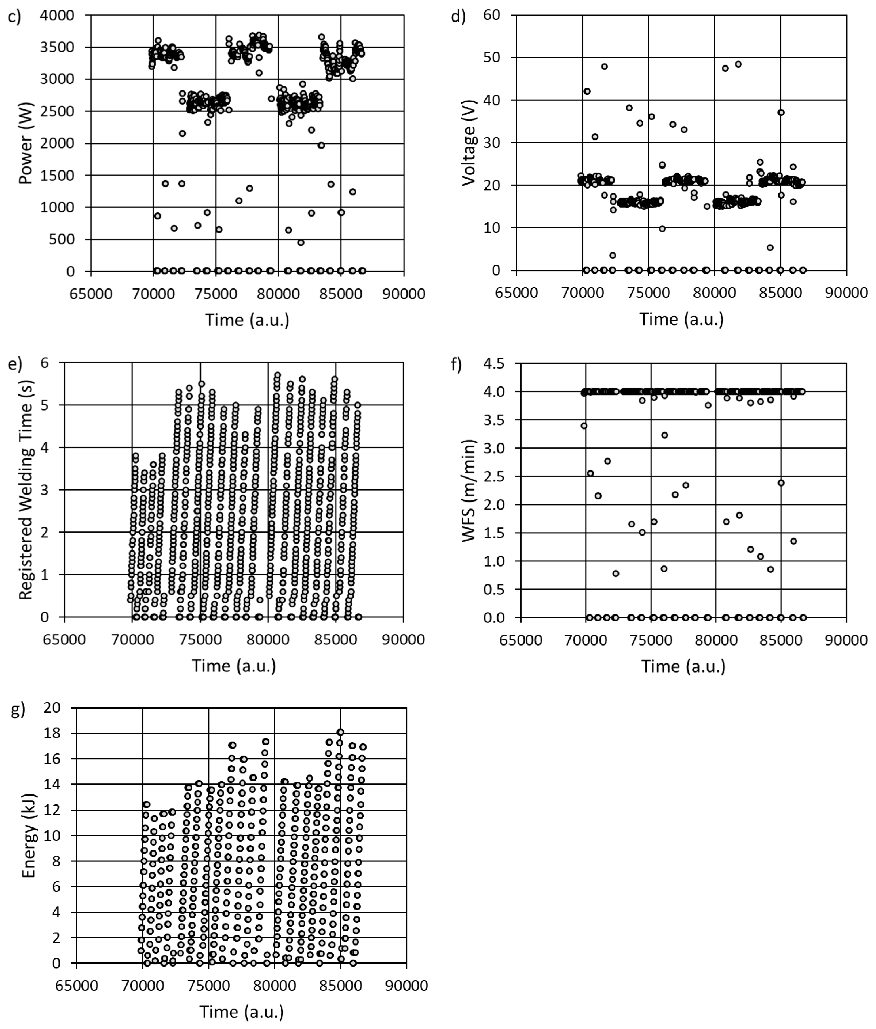
Figure 3.
Data for clusterization - different combinations of data series with time-domain excluded: power vs. current (a), voltage vs. current (b), welding time vs. current (c), WFS vs. current (d), energy vs. current (e), and energy vs. welding time (f).
Figure 3.
Data for clusterization - different combinations of data series with time-domain excluded: power vs. current (a), voltage vs. current (b), welding time vs. current (c), WFS vs. current (d), energy vs. current (e), and energy vs. welding time (f).
Figure 4.
Clusterization of data with the use of the k-means algorithm. The dependence between normalized energy and normalized current (left panel) and the dependence between overall Silhouette Value (SV) and the assumed number of clusters.
Figure 4.
Clusterization of data with the use of the k-means algorithm. The dependence between normalized energy and normalized current (left panel) and the dependence between overall Silhouette Value (SV) and the assumed number of clusters.
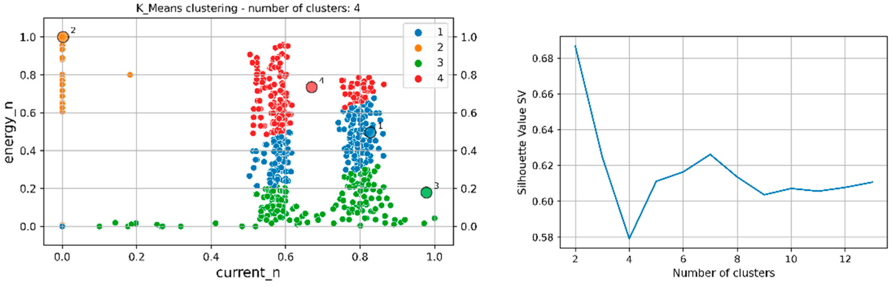
Figure 5.
Analysis of data without clustering. The relation between the normalized energy and normalized current is presented from the perspective of different welding times.
Figure 5.
Analysis of data without clustering. The relation between the normalized energy and normalized current is presented from the perspective of different welding times.
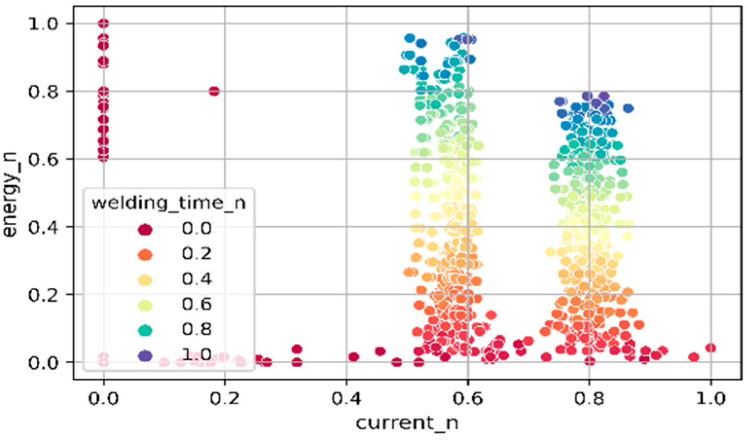
Figure 6.
Tuning of the DBSCAN algorithm – results for different minimum number of samples constituting a cluster – the choice of the region of attraction size, the epsylon range at horizontal axis.
Figure 6.
Tuning of the DBSCAN algorithm – results for different minimum number of samples constituting a cluster – the choice of the region of attraction size, the epsylon range at horizontal axis.
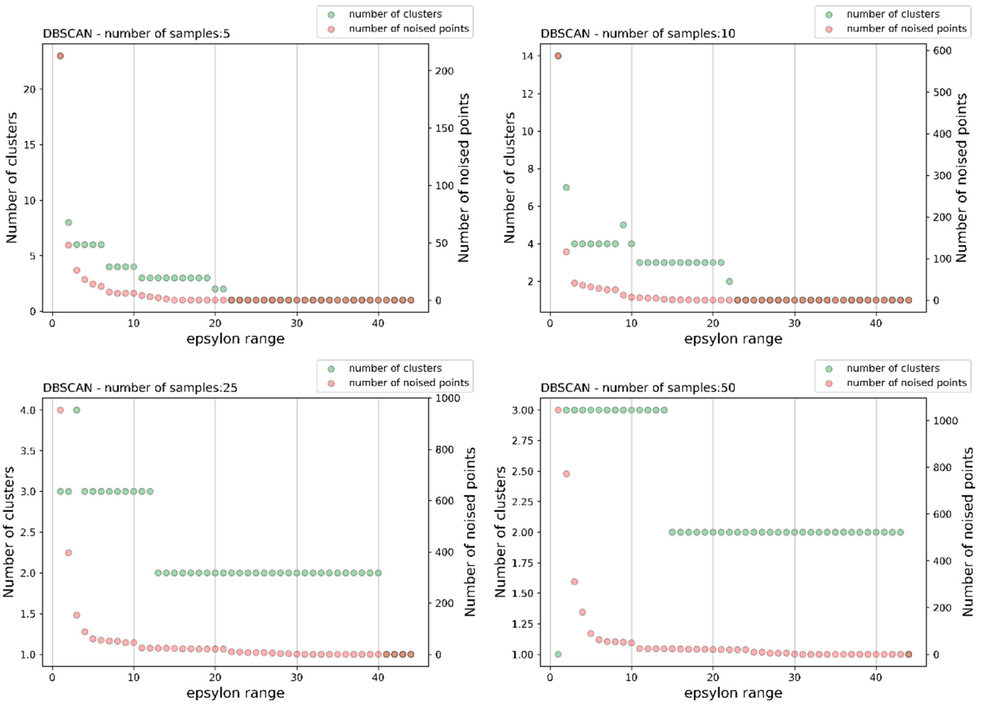
Figure 7.
Exemplary results for the DBSCAN algorithm – results for the different epsylon values (eps) equal to 5, 10, 15, 25.
Figure 7.
Exemplary results for the DBSCAN algorithm – results for the different epsylon values (eps) equal to 5, 10, 15, 25.
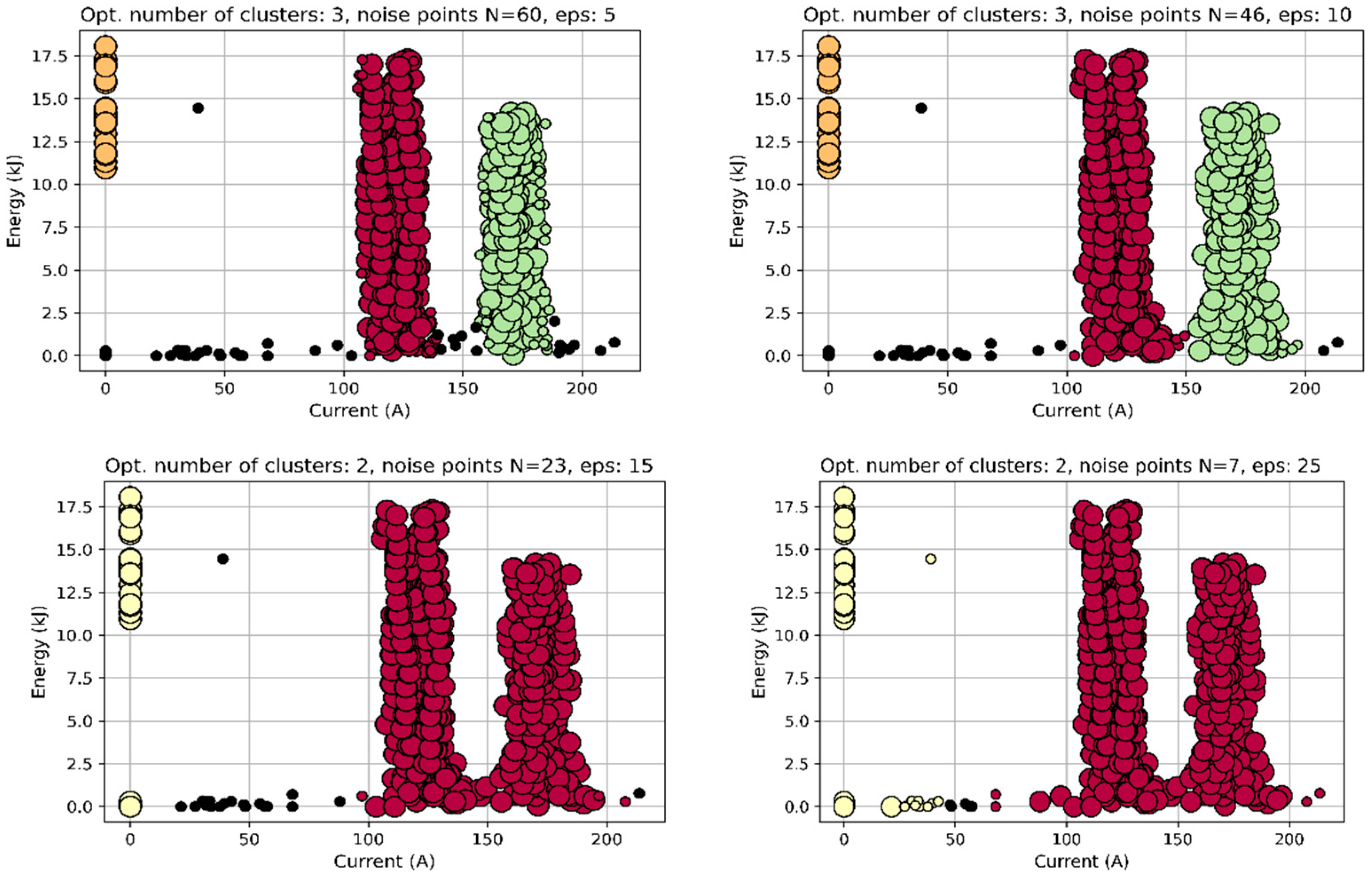
Figure 8.
Exemplary results for the HBSCAN algorithm – results for different minimum number of samples constituting a cluster – from left to right, and up to down - 15, 20, 25, 30, 40, and 80. For further evaluations the 30 samples case was chosen (marked by red frame). The graphs refer to the situation at the end of the welding process. The parameter Ns, seen above each figure, gives the number of recorded noise type points.
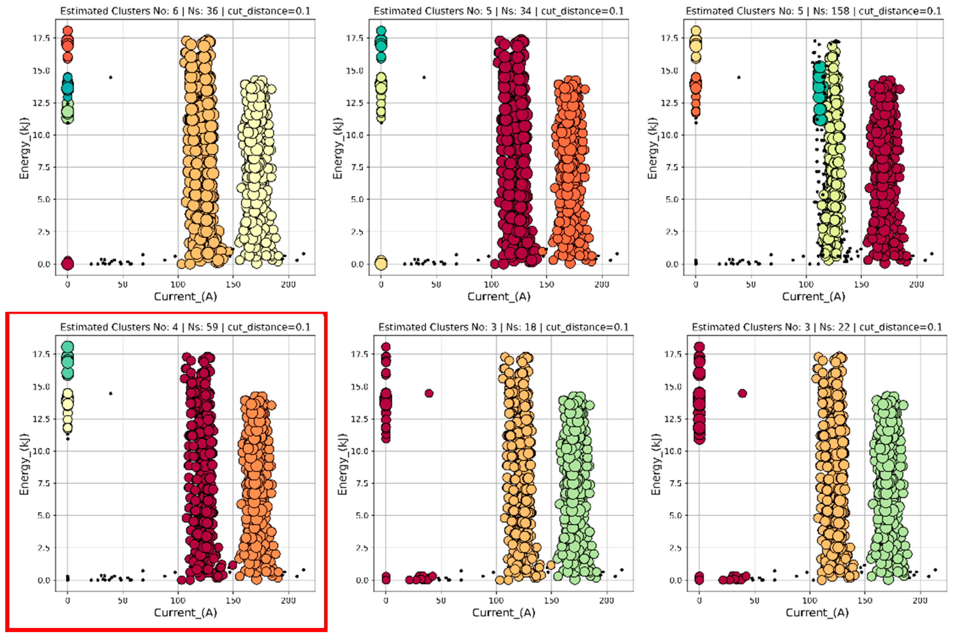
Figure 9.
Results for the HBSCAN algorithm – minimum number of samples constituting a cluster equals 30. The obtained number of clusters equals 3, 4, or 5, depending on the data series types. The figures contain all the production history, that is, they correspond to the final stage of the welding process.
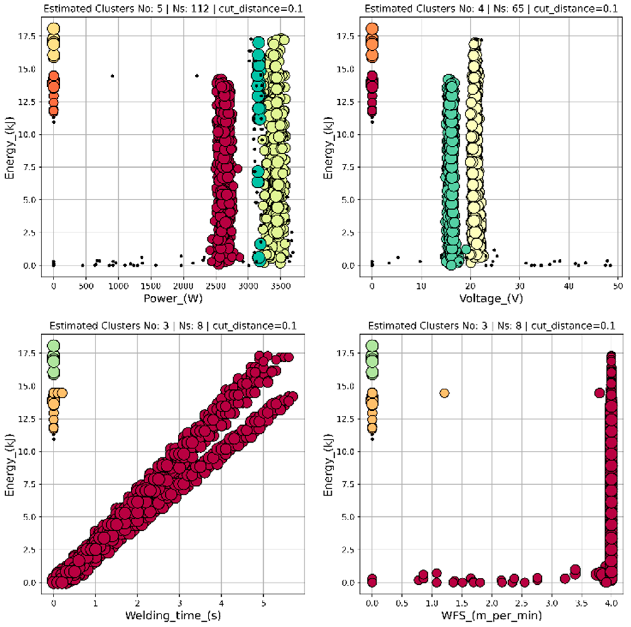
Figure 10.
Results for the HBSCAN algorithm – dynamical registration (in time) of the number of cluster and the noised points. Minimum number of samples creating a cluster equals 30. The cut distance was set to 0.1.
Figure 10.
Results for the HBSCAN algorithm – dynamical registration (in time) of the number of cluster and the noised points. Minimum number of samples creating a cluster equals 30. The cut distance was set to 0.1.
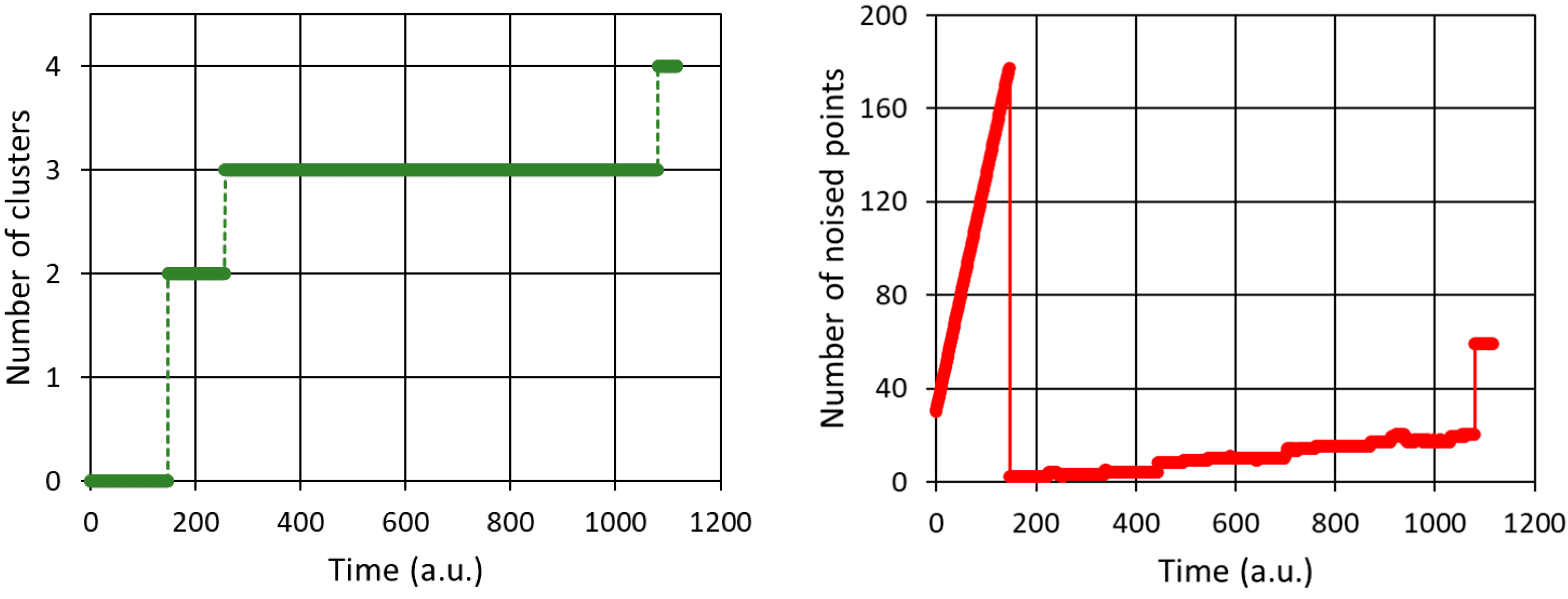
Figure 11.
Results for the HBSCAN algorithm – dynamical registration (in time) of the number of cluster and the noised points - simulation of a potential more unstable production process in comparison to results of Figure 10. The number of samples creating a cluster equals 15. The cut distance was set to 0.1.
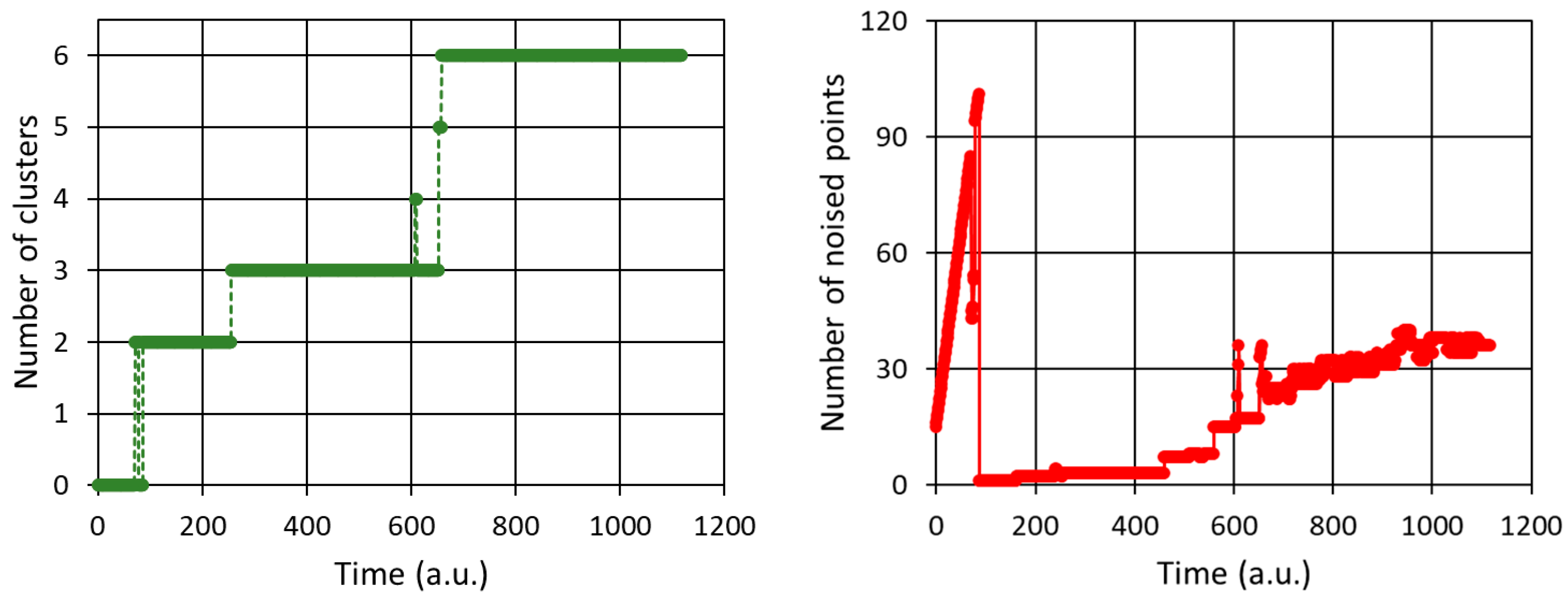
Figure 12.
Results for the HBSCAN algorithm – dynamical registration (in time) of the noised points, for different data series combinations. The number of samples creating a cluster equals 30.
Figure 12.
Results for the HBSCAN algorithm – dynamical registration (in time) of the noised points, for different data series combinations. The number of samples creating a cluster equals 30.
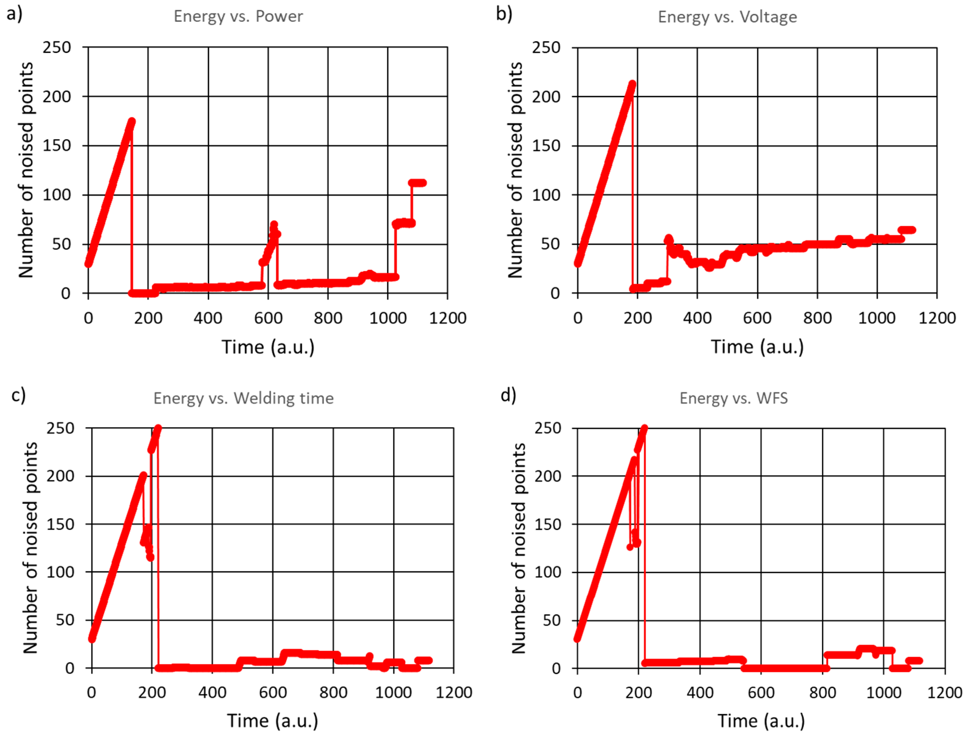
Figure 13.
1st derivative of the noise signal captured from the welding process for 30 samples to be treated as the beginning of cluster.
Figure 13.
1st derivative of the noise signal captured from the welding process for 30 samples to be treated as the beginning of cluster.
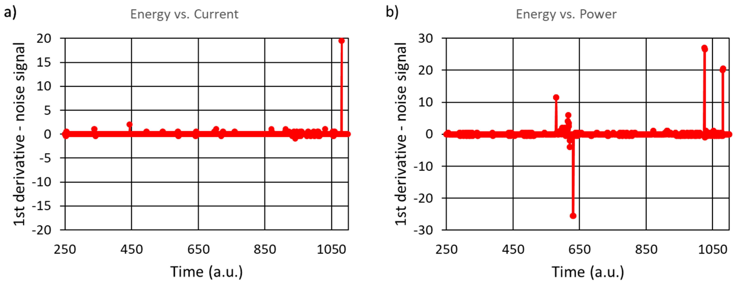
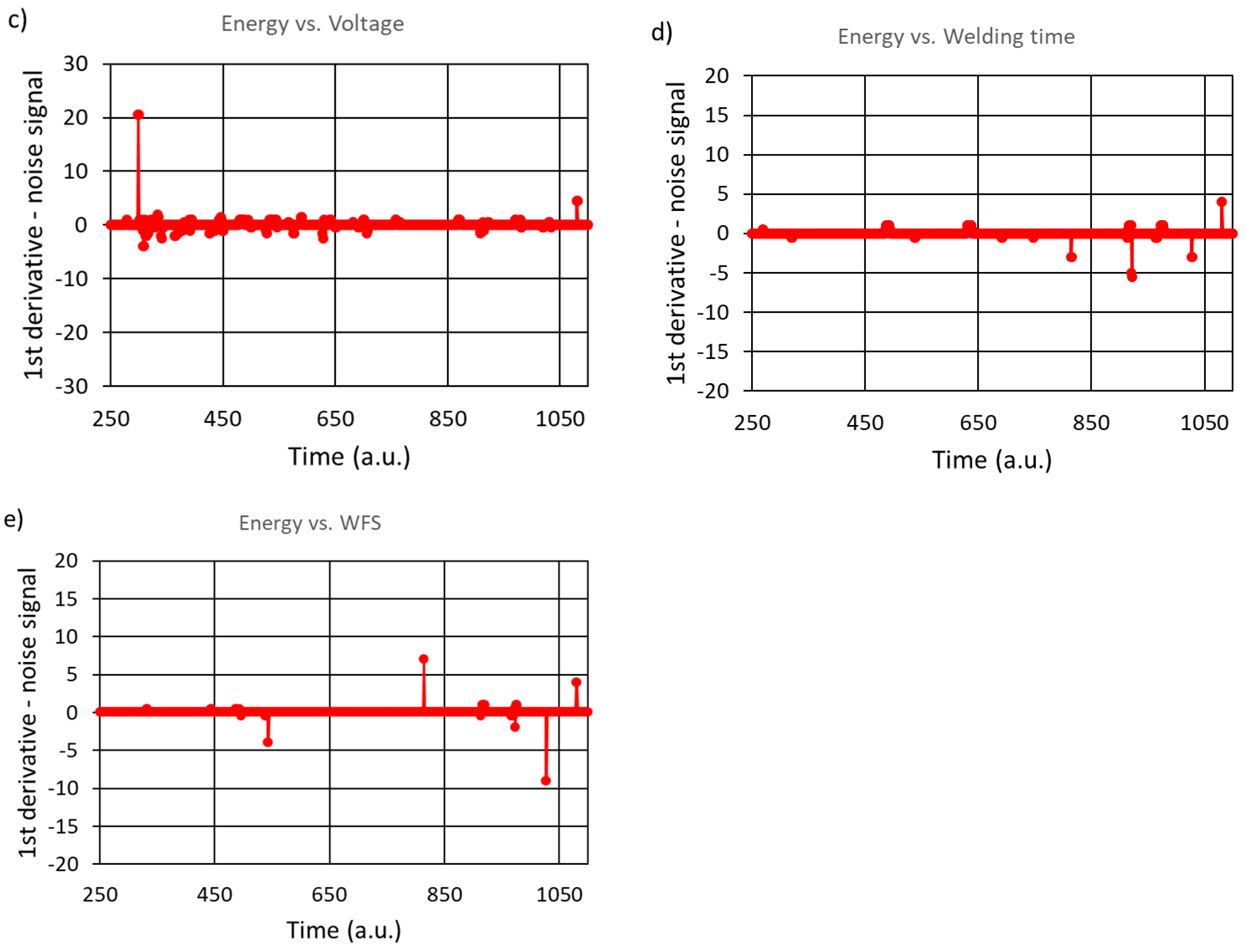
Figure 14.
Presentation of instability moments detected by the HBSCAN algorithm for energy vs. power dependence (compare Figure 13b). The instability was registered around the Time=620 moment. The left figure represents a state before increased level of noise, the right one shows the increased level of noise – the points marked by the red oval.
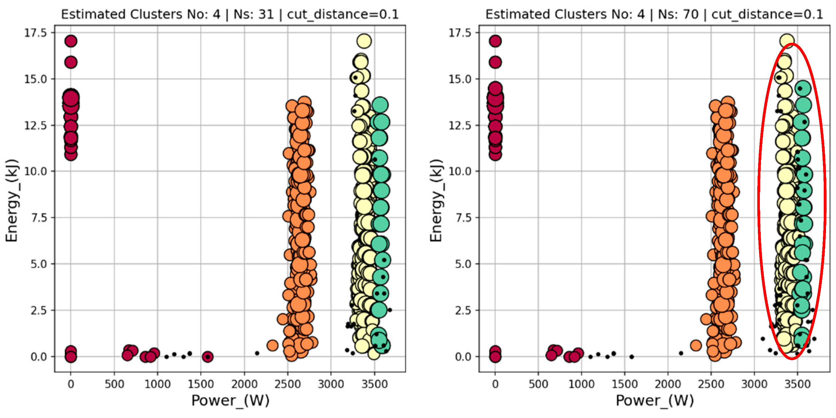
Figure 15.
Presentation of instability moments detected by the HBSCAN algorithm for energy vs. power dependence (compare Figure 13b). The instability was registered above the Time=1000 moment. The left figure represents a state before increased level of noise, the right one shows the increased level of noise – the points marked by the red oval.

Disclaimer/Publisher’s Note: The statements, opinions and data contained in all publications are solely those of the individual author(s) and contributor(s) and not of MDPI and/or the editor(s). MDPI and/or the editor(s) disclaim responsibility for any injury to people or property resulting from any ideas, methods, instructions or products referred to in the content. |
© 2024 by the authors. Licensee MDPI, Basel, Switzerland. This article is an open access article distributed under the terms and conditions of the Creative Commons Attribution (CC BY) license (http://creativecommons.org/licenses/by/4.0/).
Copyright: This open access article is published under a Creative Commons CC BY 4.0 license, which permit the free download, distribution, and reuse, provided that the author and preprint are cited in any reuse.


