
Submitted:
26 April 2025
Posted:
28 April 2025
You are already at the latest version
Abstract
Using special functions and orthogonal polynomials, we introduce an algebraic version of quantum field theory for elementary particles. Closed-loop integrals in the Feynman diagrams for computing transition amplitudes are finite. Consequently, no renormalization scheme is required in this theory.
Keywords:
quantum field theory
; algebraic system
; no renormalizatio
; Feynman diagrams
; spectral polynomials
1. Preliminaries
Quantum field theory (QFT) was developed long ago to describe elementary particles, such as the electrons and neutrons, their interaction with each other and with their environment. However, the theory had to be augmented by ad hoc rules for computing physical processes because all such computations are plagued with infinities. Up to date, all efforts to develop a practical QFT without these ad hoc rules (called renormalization) were not fully satisfactory. In this work, we attempt at a resolution of this shortcoming by introducing an algebraic version of QFT based on orthogonal polynomials and special functions that does not require renormalization. That, is a theory in which closed-loop integrals in the Feynman diagrams for calculating transition amplitudes are finite. We assume basic knowledge of QFT and thus will not dwell on a review of the theory. Interested readers may consult any of the classic textbooks on the subject such as those in Refs. [1,2,3]. Additionally, we will not assume advanced knowledge in the theory of special functions and orthogonal polynomials. It is sufficient that the reader be familiar with the properties of well-known polynomials such as the Hermite, Laguerre, Chebyshev, Gegenbauer, ...etc. At least, one must know where to find such properties by looking at any of the numerous books on orthogonal polynomials like those listed in [4,5,6,7]. For the purpose of the present development, one should be aware that an orthogonal set of polynomials has an associated weight function, satisfies a three-term recursion relation and an orthogonality.
We start by showing that the conventional representation of the free quantum field in the linear momentum space could be rewritten in an equivalent form in the energy space with an algebraic structure built on orthogonal polynomials. For example, the differential wave equation in conventional QFT becomes an algebraic three-term recursion relation satisfied by the orthogonal polynomials associated with the given quantum field. Therefore, instead of solving a differential wave equation, one can simply solve an algebraic equation. We should note, however, that the algebraic structure of this theory is fundamentally and technically different from that which is commonly known in the mathematics/physics literature as Algebraic Quantum Field Theory (AQFT). A survey of AQFT can be found in [8] and references cited therein. Next, we show that the equal-time commutation relation of the quantum field and its canonical conjugate in this equivalent algebraic theory is a direct consequence of the orthogonality of the associated polynomials and the completeness of a corresponding set of spatial functions. Additionally, we show how the basic singular two-point function, whose time ordering leads to the Feynman propagator, is constructed in a simple and transparent form using these orthogonality and completeness. Nonetheless, a free QFT (i.e., a theory without interaction) does not carry much physical significance beyond the obvious requirement of being physically and mathematically consistent and preferably elegant. Hence, we come to our most important findings where we show that closed loop integrals in the Feynman diagrams used for calculating transition amplitudes in interacting models in this algebraic theory are finite. We verify this claim in a typical model for few sample diagrams. This property relies predominantly on the orthogonality property of the associated polynomials. We give a numerical illustration showing that the finiteness property of this model continues to higher order loops. It remains to be seen whether this remarkable property is maintained in other physically relevant interaction models.
To make the presentation clear and simple, we work in 1+1 Minkowski space-time and adopt the conventional relativistic units . We do acknowledge that spinors and vector fields in such space-time may not carry much of a physical significance. However, the mathematical formulation introduced here could easily be extended to higher dimensions. Readers interested in the 3+1 space-time version of the formulation can refer to Ref. [9] for details.
2. Algebraic Structure in Conventional QFT
In conventional QFT, the positive energy component of the free quantum field associated with a scalar particle in 1+1 space-time is written as the following continuous Fourier expansion in the linear momentum k-space [1,2,3]
where the creation/annihilation field operators satisfy the commutation algebra . The free Kelin-Gordon wave equation gives the energy-momentum relation for a free particle as .
Now, it is well-known that the oscillatory function (plane wave) in Equation (1) has the following point-wise convergent expansion
where is the Hermite polynomial of degree n in y, and λ is an arbitrary scale parameter with the dimension of energy. Applying the differential operator on this expression and using the differential equation of the Hermite polynomial, , we get
where . To compute the term , we repeat the recursion relation of the Hermite polynomial, , twice resulting in
Therefore, if we write where or , then becomes a linear combination of and with constant coefficients that depend on the index n. That is, results in a three-term recursion relation for that can be made symmetric by adopting the following normalization
Consequently, we can write
for and where
Therefore, if we write the series (2) as follows
then with or , and Equation (4) becomes
Making the replacement and in the second and third terms in the sum, respectively, we obtain
for . We write making . Therefore, the free Klein-Gordon wave equation becomes the following algebraic three-term recursion relation
where and making a polynomial in z of degree n. In fact, one can easily verify that (where or )1 solves the recursion (11). We call the “spectral polynomials” and z the “spectral parameter”. Using the orthogonality of the Hermite polynomials, , we obtain the following orthogonality of the spectral polynomials
where is the associated weight function that reads , which is positive definite for , and . Therefore, given the algebraic structure defined by the spectral polynomials and the associated complete spatial functions , we can rewrite the quantum field (1) as
In Appendix A, we give another representation equivalent to (13) but with a different set of spectral polynomials (the Gegenbauer polynomials) and spatial functions (the Bessel functions). Inspired by these expansions and the algebraic structure associated with the spectral polynomials, we consider in the next section the following quantum field representation, which is an E-space equivalent to the k-space representation (1) or (13), that reads
where , and to be determined. Based on this (and other similar) mapping of the quantum fields from the k-space to E-space using such an expansion, we present in the following section a systematic formulation of our proposed algebraic QFT.
3. The Algebraic QFT
In this proposed theory, the positive energy component of the scalar quantum field in 1+1 Minkowski space-time is represented by the following continuous Fourier expansion in the energy
where and making . are real and dimensionless set of functions of the spectral parameter z whereas is operator-valued (the annihilation operator) that satisfies the following commutation algebra
where the function is positive definite to be determined below by canonical quantization. Consequently, unlike the conventional theory where the operator creates/annihilates the entire quantum field, here creates/annihilates a single spectral mode (the nth mode) of the quantum field. is a complete set of spatial functions in configuration space that satisfy the following differential relation
where is a universal constant of inverse length dimension (a universal scale/mass). The coefficients are real dimensionless parameters that are independent of the energy and such that for all n. Using (17), the free Klein-Gordon wave equation becomes the algebraic relation (11) for and with . Equation (11) is a symmetric three-term recursion relation that makes a sequence of polynomials in z with the two initial values and a two-parameter linear function of z. Now, Equation (11) has two linearly independent polynomial solutions. We choose the solution with the initial values and . The spectral theorem (a.k.a. Favard theorem) [4,5,6,7] states that the polynomial solutions of the recursion (11), with the recursion coefficients being positive definite, must satisfy the orthogonality relation (12) with being the associated weight function, which is positive definite and will be related to by canonical quantization. The fundamental algebraic relation (11), which is equivalent to the free Klein-Gordon wave equation, is the reason behind the algebraic setup of the theory and for which we qualify this QFT as algebraic. In fact, postulating the three-term recursion relation (11) eliminates the need for specifying a free field wave equation. Furthermore, once the set of spectral polynomials is given then all physical properties of the corresponding particle are determined.
Now, the conjugate quantum field is obtained from (15) by complex conjugation and the replacement where the pair satisfy the following orthogonality and completeness relations
Therefore, we write as
Using the commutators of the creation/annihilation operators shown above as Equation (16) and noting that , we can write
The orthogonality (12) and the completeness (18b) turn this equation with into
provided that we take , which makes the commutation (16) read as follows
Moreover, it is straightforward to write
In the canonical quantization of fields [1,2,3], equations (21) and (23) give the canonical conjugate to as . Moreover, in analogy with conventional QFT [1,2,3], we can write Equation (20) as
giving the singular two-point function as follows
Moreover, Equation (21) and Equation (25) give: . The vacuum expectation of the time ordered gives the Feynman propagator . Therefore, the elements needed to define the free sector of this algebraic theory are: the spectral polynomials and the spatial set of functions together with their conjugates .
It is interesting to note that if we identify the scalar quantum field given by the conventional representation (1) with the new algebraic representation (15), then using the expansion (2) we obtain: , as given by Equation (5), and . Hence, we obtain the annihilation operator map between the two representations where and we have used the on-shell relation for free fields.
A real (neutral) scalar particle in 1+1 space-time is represented by the quantum field with . On the other hand, a complex (charged) scalar particle is represented by a quantum field whose positive-energy component is and its negative-energy component is where is identical to (15) but with the associated spectral polynomials along with their recursion coefficients , weight functions , and with the annihilation operators that satisfy where r and stand for ±.
The particle propagator is an operator that takes the particle from the space-time point to with . In other words, the particle is created from vacuum at then annihilated later at . In the algebraic formulation, the equivalent “spectral propagator” reads where is the vacuum. Now, since , then we can write
We designate the spectral propagator by that takes [more precisely, ]. That is, the propagator must satisfy
The orthogonality (12) shows that the representation satisfies (27). This is also suggested by the two-point function of equation (26) that could be rewritten as follows
Consequently, is the propagator for individual spectral modes of the quantum field () leaving other modes unaffected, which is unlike in the conventional theory where the entire quantum field is propagated. Moreover, using the completeness of the spectral polynomials that reads , one can also show that this propagator has the property . Furthermore, using the orthogonality (12), it is evident that . Additionally, it has the exchange symmetry . Energy conservation, on the other hand, which is evident by the presence of the Dirac delta function in the propagator equation (26), implies that . In the following Section, we show how this propagator enters in the calculation of the scattering amplitudes via the Feynman diagrams.
4. Interaction in the Algebraic QFT
In this Section, we show how to calculate the scattering amplitude in a generic interaction model. We consider the interaction Lagrangian and choose to be a scalar, a spinor2, and a dimensionless coupling tensor of rank three that couples individual spectral field modes. This interaction Lagrangian resembles that of QED where the scalar field is replaced by the massless vector field (the photon). If we designate as the set of spectral polynomials associated with the spinor component , then we can write the corresponding spinor annihilation operators and their anti-commutation relation where and is the spinor weight function. For simplicity, we consider neutral particles and a single spinor component where we can write
where is the two-component spinor basis functions that satisfy equations (B5) and (B9) in Appendix B of Ref. [9]. The fermionic structure of the interaction dictates that the coupling tensor is antisymmetric in the fermionic indices. That is, .
As illustrative example of calculating the scattering amplitudes, we start by considering the first order (one-loop) correction to the free propagator (i.e., self-energy). Figure 1 represents the associated Feynman diagram in this model where the propagator for the scalar (spinor) is represented by a dashed (solid) curve. In the following figures, we designate the spectral propagator for the spinor as with and for the scalar as with . Note that conservation of energy gives .
.
Since the spectral polynomials carry a faithful representation of the quantum field, we adopt the notation for the amplitude shown in the Figure with . Moreover, the spinor propagator for the top part of the closed loop is with whereas for the bottom part it reads with
and (i.e., the signs of E and are the same) since w should be positive. In the algebraic system introduced in Ref. [10], the spectral parameter addition (30) is written as . Therefore, to compute the amplitude of Figure 1, we integrate over all possible values of u and sum over all possible indices (polynomial degrees) . That is, to first order, we obtain the following spectral propagator for the scalar particle
The integral in this amplitude is one of the “fundamental SAQFT integrals” introduced in Ref. [9] and denoted by for and (i.e., for “monochrome propagation”). In general, transition amplitudes like (31) are written as where is the term (or sum of terms) in the perturbation series that corresponds to a Feynman diagram (or rather topologically distinct Feynman diagrams) with n vertices and m loops.3 Therefore, in (31) and whereas is the second term in (31). The finiteness of the scattering amplitude is two-fold; one for integrals and another for sums. The first, is the finiteness of the integral, which is guaranteed by the orthogonality (12) of the spectral polynomials. In fact, we have shown in [9] that the value of falls within the interval [0,1] for all spectral polynomials satisfying the orthogonality (12). Moreover, its value goes to zero fast enough if any of the indices i or j go to infinity. The second issue in the finiteness of the scattering amplitude is the convergence of the series shown in Equation (31), which depends on the asymptotics and sign signature of the components of the coupling tensor .
In the integral of Equation (31), the spectral parameter u assumes values that correspond to all possible ranges of the energy (i.e., and ). Therefore, the integral runs over all positive values of u from 0 to since . In the following section, we give a numerical illustration of the finiteness of the scattering amplitude (31) and show that monochrome propagation enhances the scattering amplitude. Additionally, we compute a truncated version of the series in (31) demonstrating converges as the number of terms increase.
The second order (two-loop) correction to the scalar propagator contains several diagrams one of which is shown below as Figure 2. To compute this second order correction, we integrate over all possible values of u and w and sum over all possible indices and . To simplify, we assume monochrome propagation where the degrees of the spectral polynomials are preserved in propagation. That is, and . In the diagram of Figure 2, this is equivalent to the replacement and . Accordingly, we obtain the following second order contribution to the self-energy of the scalar propagator
Where
In the following section, we evaluate the double integral (32) for a given range of the scalar energy and a fixed set of the polynomial degrees and show that the value of the integral diminishes as the indices (or some of them) become large.
Finally, we consider the first order correction to the interaction vertex in this model. The associated Feynman diagrams are many (in fact, there are six topologically distinct diagrams). We consider here one of these diagrams, which is shown below as Figure 3 where the spectral parameters are related by the energy conservation as . The bare vertex is just the coupling tensor element independent of the energy. On the other hand, the value of the diagram in Figure 3 reads as follows:
For monochrome propagation, , , and , this expression simplifies to read:
In the following section, we show that the value of the integral in (35) falls within the range [0,1] and diminishes rapidly as the polynomial degrees increase.
5. Numerical Results
In this section, we evaluate the transition amplitudes presented in the previous section by the sample Feynman diagrams of Figure 1, Figure 2 and Figure 3. The results demonstrate finiteness of the closed-loop integrals for this model in our proposed algebraic QFT. For the purpose of calculation, we choose the model parameters as follows. We take a massless scalar () where the associated spectral polynomials is the even Hermite polynomial . The spectral polynomial associated with the massive spinor is taken as the Laguerre polynomial with . Now, it is well-known that the odd/even Hermite polynomials could be expressed in terms of the Laguerre polynomials. That is, we can write . Therefore, the orthonormal spectral polynomials, their normalized weight function and recursion coefficients associated with the scalar are as follows:
where . On the other hand, for the spinor they read:
where . In the calculation, we take and . Moreover, the elements of the coupling tensor are written in terms of the recursion coefficients (36b) and (37b) as follows
where is a dimensionless coupling parameter. For a given set of indices , we evaluate the integral in (31) that reads
with . To evaluate the integral, we use Gauss quadrature integral approximation (see, for example, Ref. [11]). In such calculation, we start by computing the eigenvalues and normalized eigenvectors of an tridiagonal symmetric matrix J whose diagonal elements are and off-diagonal elements are , where M is the order of the quadrature such that and are those given by (37b). If we call such eigenvalues and the corresponding normalized eigenvectors , then the integral (39) is approximated as follows
where is an diagonal matrix whose elements are
Figure 4 shows the result of such an evaluation for a given range of the scalar energy . Figure 5 is a plot of in colors corresponding to monochrome propagation superimposed by several polychrome propagation in black. This figure shows that monochrome propagation is (as expected) positive definite boosting the value of the sum in (31) whereas polychrome propagation results in cancellations enhancing fast convergence of the sum. It is also evident from these figures that the magnitude of the integral (39) is less than one. In Appendix B, we use a linearization technique [12] to simplify the polynomial product in the integral (39).
Moreover, to demonstrate convergence of the calculation of the transition amplitude (31), we evaluate the same self-energy diagram to first order for a fixed energy and polynomial degrees n and m but as a function of the number of terms N in the sum
Figure 6 illustrates convergence of the series as N increases where we took . Figure 7 is a reproduction of Figure 6 after imposing monochrome propagation where . Therefore, the scalar propagator could be written to first order as follows:
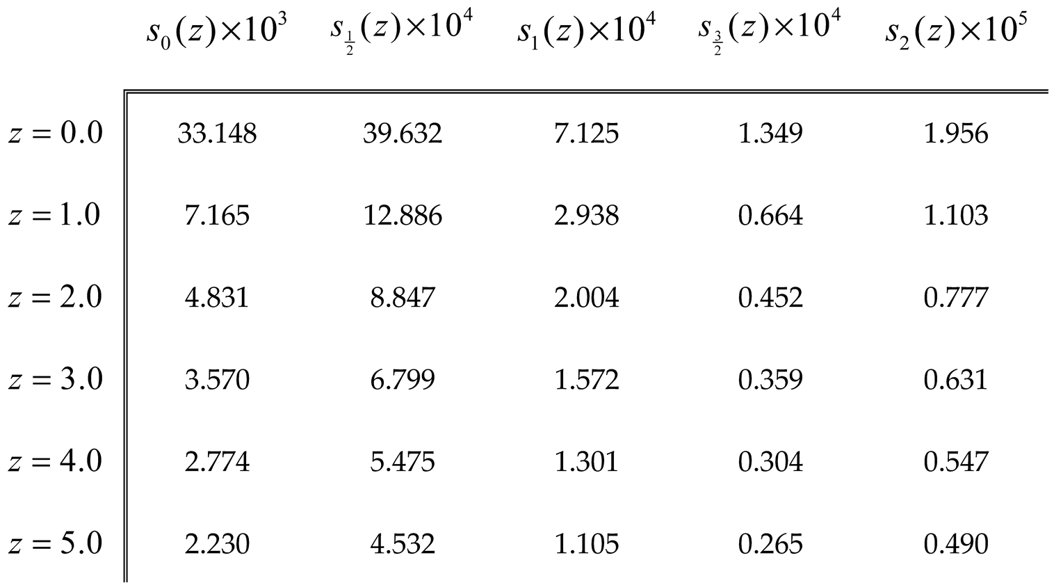
where could be interpreted as the square of the energy dependent coupling parameter of the model. Table 1 is a list of for monochrome propagation and for several values of the energy and spinor parameter .
If we repeat the same self-energy calculation but for the spinor propagator, we obtain the following result to first order
Next, we evaluate the double integral associated with the diagram of Figure 2 for mono-chrome propagation and given by Equation (32) that reads
where , and . Figure 9 is a plot of for a given set of indices and range of scalar energy. The figure is a superposition of three evaluations of the integral using an increasing order of Gauss quadrature: 15 (dashed red), 30 (dotted blue), and 60 (solid black).
Figure 10 is a reproduction of Figure 9 (with a Gauss quadrature order of 60) but for large values of the indices (10 times those of Figure 9). The figure demonstrates diminishing values for the integral (of the order of 200 times less). For this latter calculation, we used the large degree asymptotics of the Laguerre polynomials to write
where we have used .
6. Conclusions
We have presented in this study an algebraic version of QFT that utilizes the theory of orthogonal polynomials and where we adopt a representation of the quantum fields in the energy rather than linear momentum space. The quantum fields in this theory are created, annihilated and propagated on the level of individual spectral modes of the field rather than in totality as in the conventional QFT. The differential wave equation for the free quantum field in conventional QFT is replaced by an algebraic three-term recursion relation for the associated spectral polynomials. The proposed theory is, in fact, the structureless version of SAQFT that was introduced recently in [9]. We presented several examples in a typical interaction model illustrating the remarkable property that the theory is finite eliminating the need for renormalization altogether. It remains to be seen whether this finiteness property prevails in other physically relevant models within this algebraic QFT.
Finally, we like to point out that the work presented here should be considered the start of the development of a robust algebraic quantum field theory of elementary particles that does not require renormalization. The results presented in this study indicate that such a theory does indeed exist and it is a viable alternative to the conventional formulation of QFT.
Acknowledgement
We are grateful to Dr. A. Bahaoui and the theoretical physics group lead by Prof. A. Jellal at Chouaib Doukkali University in El Jadida, Morocco for assistance in the numerical calculations leading to the result shown in Figure 6.
Appendix A: Other Equivalent Algebraic Representations
If the one-dimensional configuration space is the semi-infinite line (e.g., the radial coordinate ), then a more appropriate representation of reads as follows (see, for example, Equation (4.8.3) in Ref. [7])
where is the Gegenbauer (ultra-spherical) polynomial, is the Bessel function of the first kind and the parameter is positive. Applying the differential operator on this expression and using the differential equation of the Bessel function, , we get
where and . To compute the first two terms inside the square brackets, we use the following differential property and recursion relation of the Bessel function
Consequently, Equation (A2) becomes
Making the replacement and in the second and third sum, respectively, we obtain
Iterating the recursion relation of the Gegenbauer polynomial, , twice shows that the three terms inside the square brackets add up to giving , as expected. Therefore, in the sum (A1) and with , we can identify the polynomial with where or . However, to make the corresponding three-term recursion relation symmetric as in (11) and the orthogonality normalized as in (12), we use the orthonormal version of the Gegenbauer polynomial and thus write
with or and the recursion coefficients become
Using the orthogonality of the Gegenbauer polynomials, , we obtain the normalized weight function
Therefore, in the expansion (A1), we can take and where or .
A more general expansion formula was established by Fields and Wimp in [13] which was generalized by Verma in [14] and written as Equation (9.0.10) in the book by Ismail [7]. Making the choices , , , , and in Equation (9.0.10), we obtain
where is the Pochhammer symbol, which is also known as the shifted factorial, and we used the identity for . However, if we exchange the choices for and then we obtain
Appendix B: Simplifying the Fundamental SAQFT Integrals Using Polynomial Product Linearization
In this Appendix, we use a linearization technique for the products of orthogonal polynomials [12] to simply the fundamental SAQFT integrals. Specifically, we apply this technique to the integral of Equation (39). In Ref. [12], Theorem 1 states that if the orthogonal polynomials satisfy the symmetric three-term recursion relation (11) and orthogonality (12), then the product of two such polynomials could be linearized as follows
where and J is a tridiagonal symmetric matrix whose diagonal elements are and off-diagonal elements are . Moreover, for and for . Therefore, the sum in (B1) can start from zero up to any integer greater than or equal to . Consequently, using (B1), we can write (39) as follows
and we call the “abbreviated SAQFT integral”. Additionally, we can write the partial sum (41) as follows
where “tr” is the trace of the matrix inside the square brackets.
Using Gauss quadrature integral approximation of order M (with ) we can write as follows
where is a diagonal matrix whose elements are and is an eigenvalue of the matrix J with the corresponding normalized eigenvector . An alternative Gauss quadrature approximation with a reduced order M () could be used in which we can write as
where or
with being the set of eigenvalues of the matrix obtained from J by deleting the first (zeroth) row and first (zeroth) column.
References
- J. D. Bjorken and S. D. Drell, Relativistic Quantum Fields (McGraw-Hill, 1965).
- C. Itzykson and J. B. Zuber, Quantum Field Theory (McGraw-Hill, 1980).
- M. E. Peskin and D. V. Schroeder, An Introduction to Quantum Field Theory (CRC Press, 2019).
- G. Szegő, Orthogonal Polynomials (American Mathematical Society, 1939).
- T. S. Chihara, An Introduction to Orthogonal Polynomials (Dover, 2011).
- G. E. Andrews, R. Askey and R. Roy, Special Functions (Cambridge University Press, 2001).
- M. E. H. Ismail, Classical and Quantum orthogonal polynomials in one variable (Cambridge University press, 2009).
- H. Halvorson and M. Mueger, Algebraic Quantum Field Theory, arXiv:math-ph/0602036. [CrossRef]
- D. Alhaidari, Structural Algebraic Quantum Field Theory: Particles with structure, Phys. Part. Nuclei Lett. 20 (2023) 1293.
- D. Alhaidari and A. Laradji, A Novel Algebraic System in Quantum Field Theory, AppliedMath 3 (2023) 461.
- D. Alhaidari, Gauss Quadrature for Integrals and Sums, Int. J. Pure Appl. Math. Res. 3 (2023) 1.
- D. Alhaidari, Exact and simple formulas for the linearization coefficients of products of orthogonal polynomials and physical application, J. Comput. Appl. Math. 436 (2024) 115368.
- J. Fields and J. Wimp, Expansions of hypergeometric functions in hypergeometric functions, Math. Comp. 15 (1961) 390.
- Verma, Some transformations of series with arbitrary terms, Ist. Lombardo Accad. Sci. Lett. Rend. A 106 (1972) 342.
| 1 | A more proper identification is to write these spectral polynomials in terms of the Laguerre polynomials as instead of and . As such, we can write the associated recursion coefficients as , , and the associated weight functions . |
| 2 | see Appendix B in Ref. [9] for the construction of the spinor quantum field in this algebraic QFT. |
| 3 |
m loops mean integrations over m independent spectral parameters. |
Figure 1.
Feynman diagram for the first order (single loop) correction to the scalar propagator (i.e., self-energy) in the model
Figure 1.
Feynman diagram for the first order (single loop) correction to the scalar propagator (i.e., self-energy) in the model
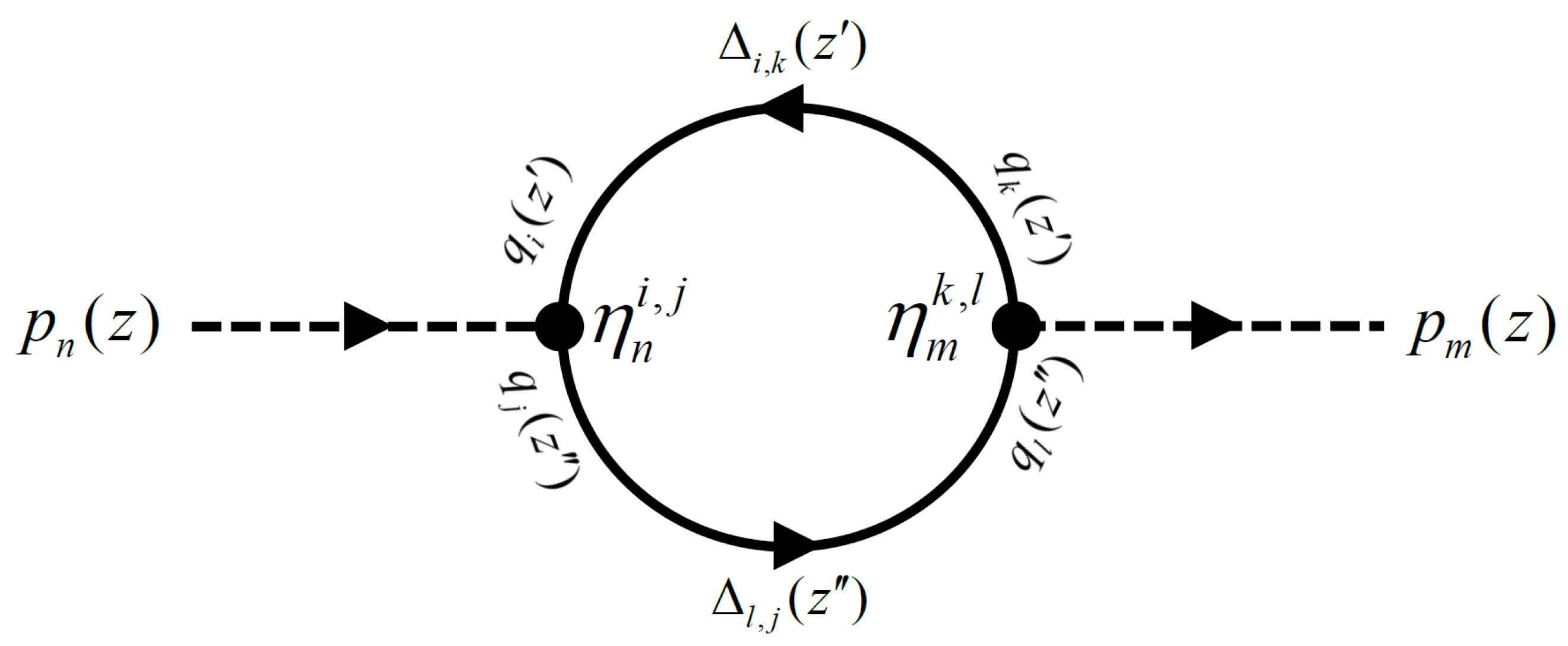
Figure 2.
One of the Feynman diagrams contributing to the second order (two-loop) correction to the scalar propagator (i.e., self-energy) in the model .
Figure 2.
One of the Feynman diagrams contributing to the second order (two-loop) correction to the scalar propagator (i.e., self-energy) in the model .
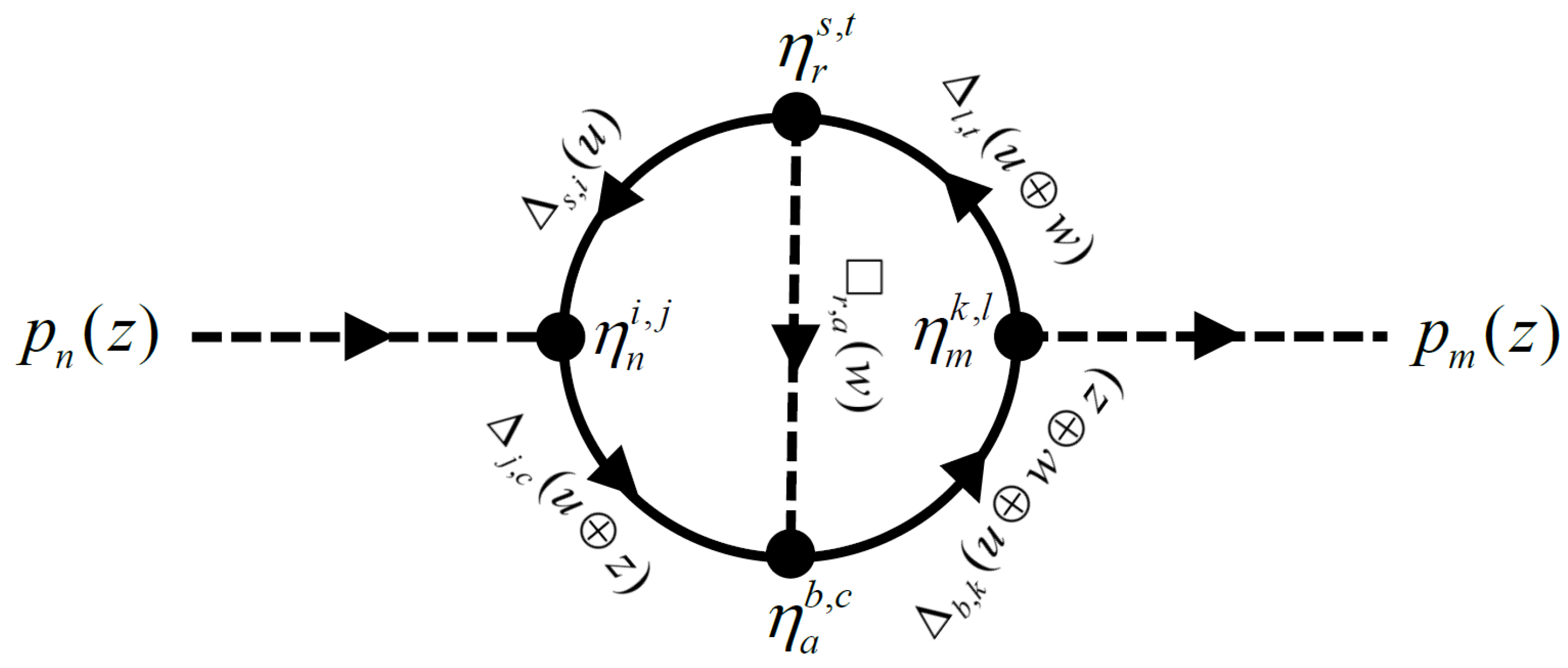
Figure 3.
One of the Feynman diagrams contributing to the first order (one-loop) correction to the interaction vertex in the model .
Figure 3.
One of the Feynman diagrams contributing to the first order (one-loop) correction to the interaction vertex in the model .
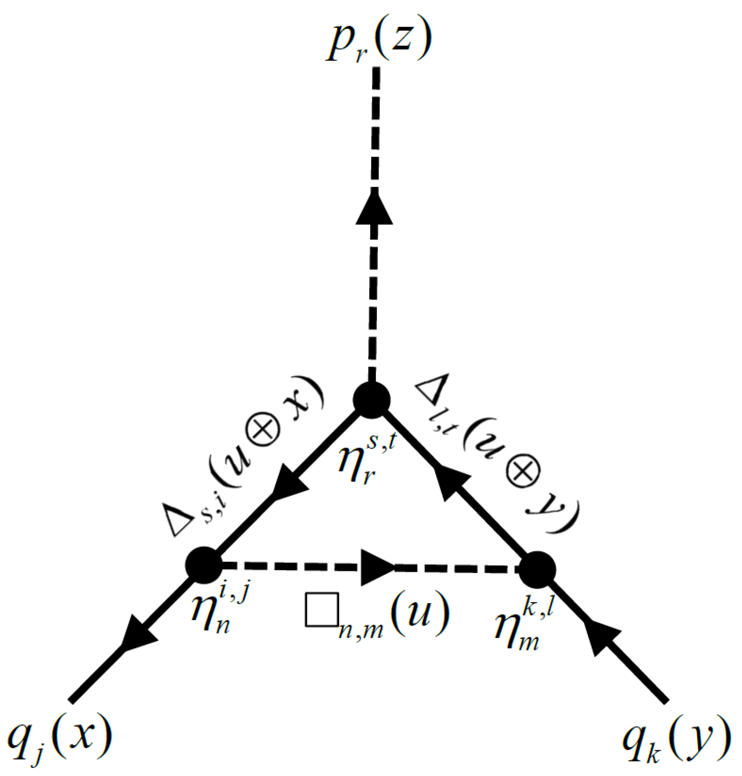
Figure 4.
Gauss quadrature approximation of the integral (39) with a quadrature order of 100.
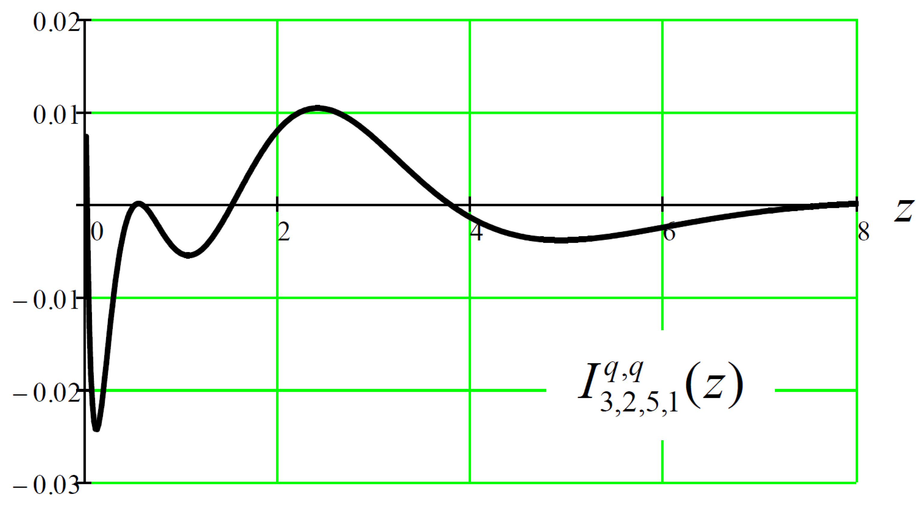
Figure 5.
Plot of the integral (39) corresponding to monochrome propagation as in red, in green, in blue, and in brown. Plots in black correspond to polychrome propagation for , , , and .
Figure 5.
Plot of the integral (39) corresponding to monochrome propagation as in red, in green, in blue, and in brown. Plots in black correspond to polychrome propagation for , , , and .
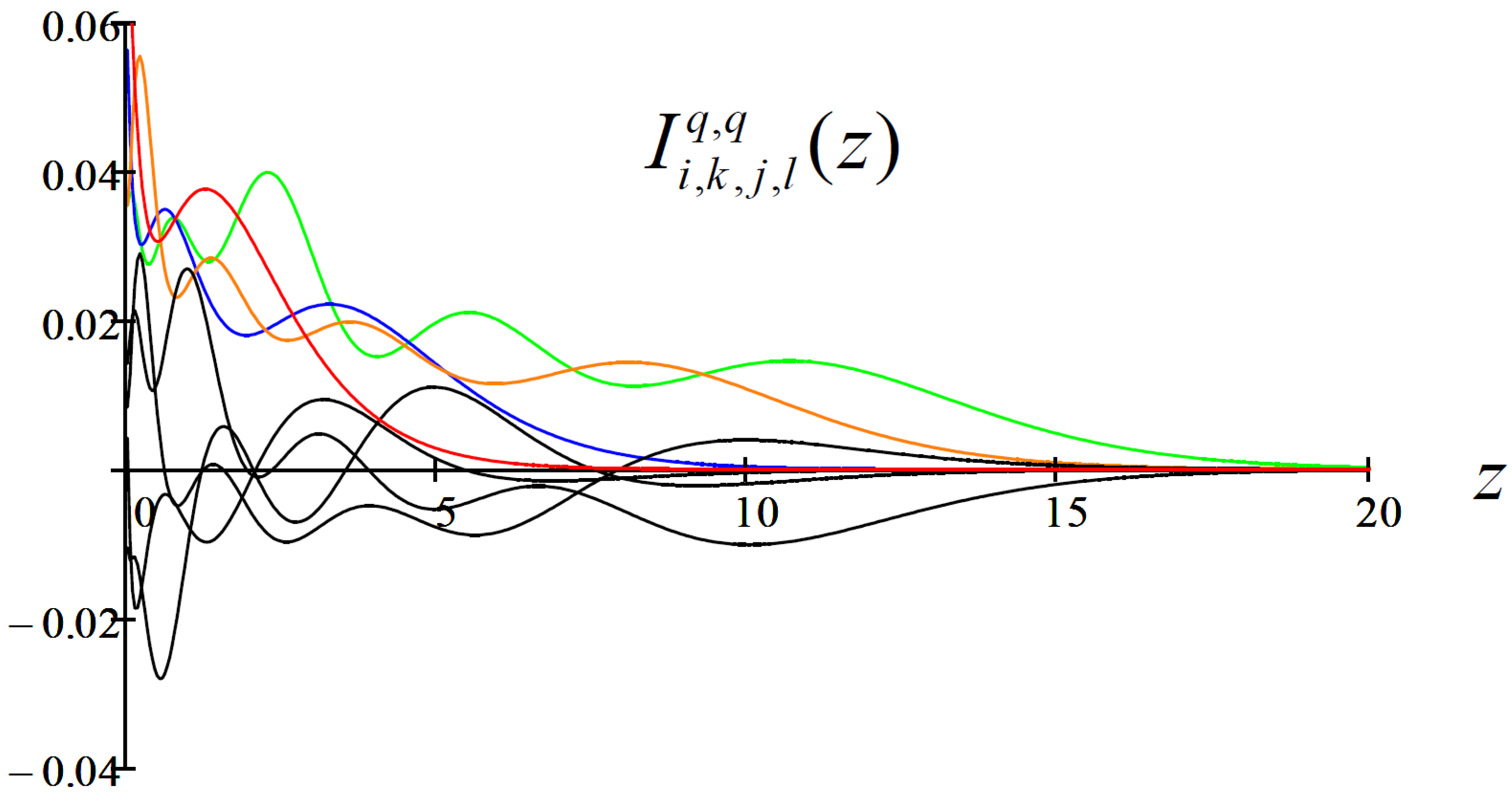
Figure 6.
The partial sum defined by Equation (41) for , , , and . The elements of the coupling tensor in this model are given by Equation (38).
Figure 6.
The partial sum defined by Equation (41) for , , , and . The elements of the coupling tensor in this model are given by Equation (38).
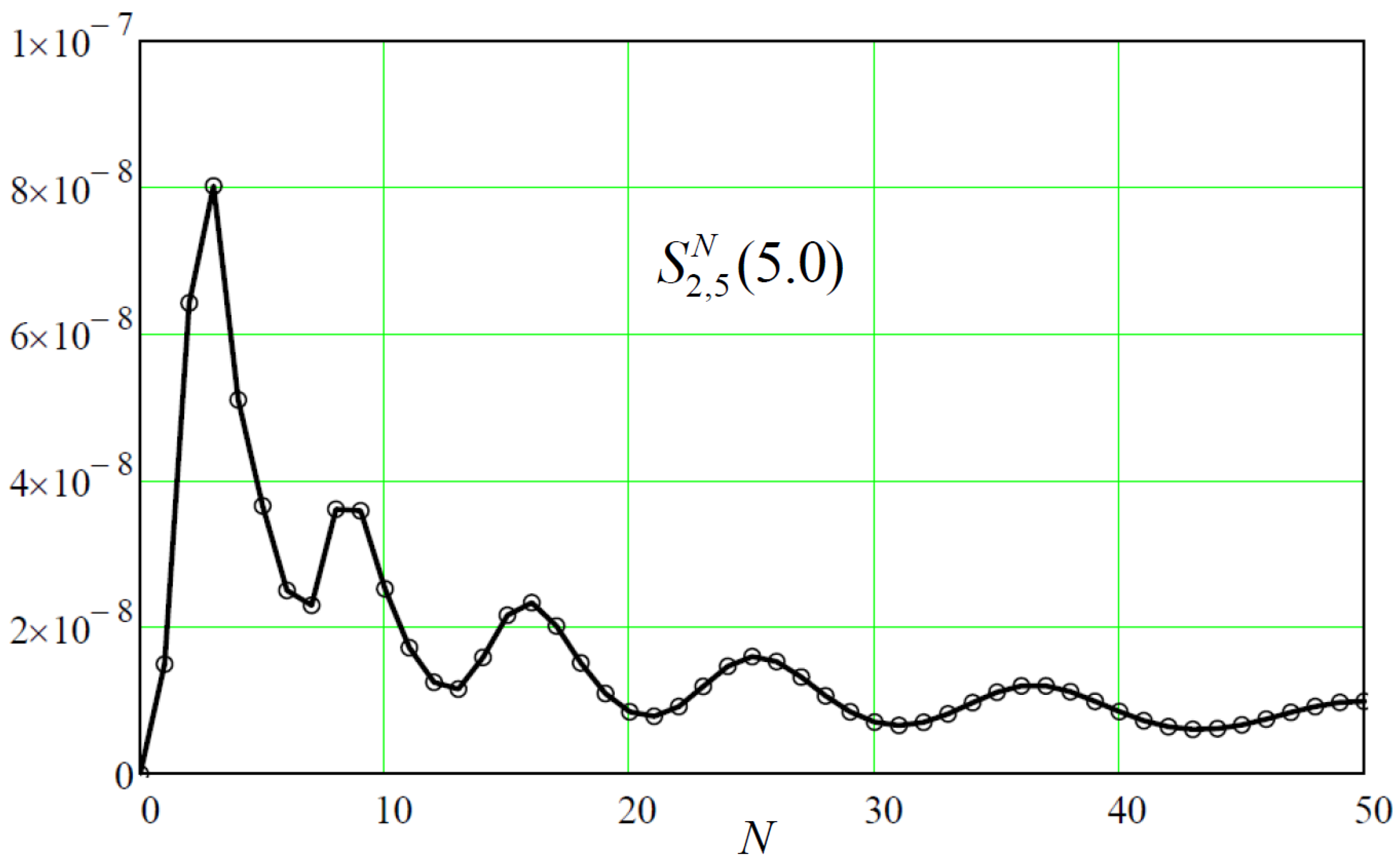
Figure 7.
Reproduction of Figure 6 after imposing monochrome propagation.
Figure 7.
Reproduction of Figure 6 after imposing monochrome propagation.
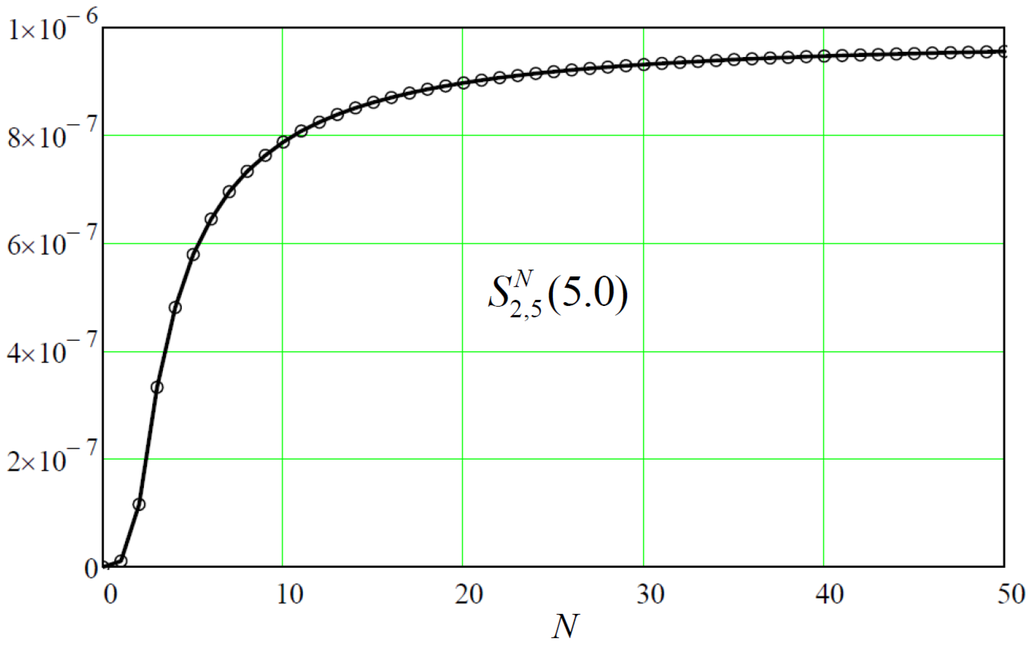
Figure 8.
Reproduction of Figure 4 and Figure 5 for the spinor particle: (a) polychrome propagation, (b) monochrome propagation.
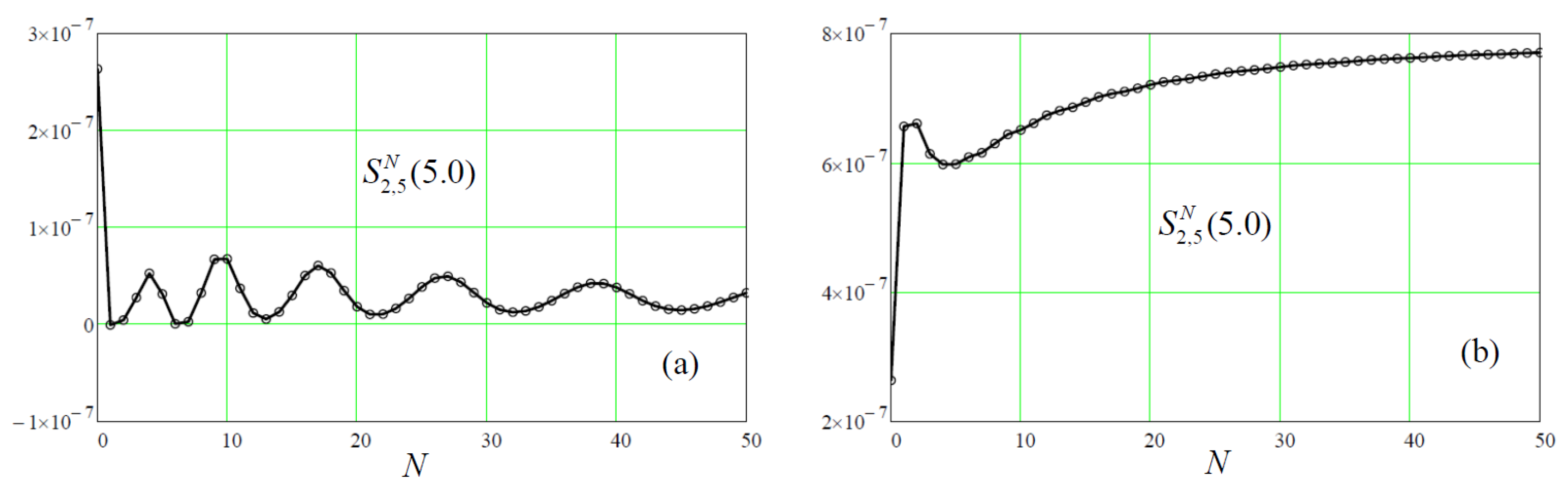
Figure 9.
Plot of the integral (44) demonstrating convergence by increasing the Gauss quadrature order from 15 (dashed red), to 30 (dotted blue), to 60 (solid black).
Figure 9.
Plot of the integral (44) demonstrating convergence by increasing the Gauss quadrature order from 15 (dashed red), to 30 (dotted blue), to 60 (solid black).
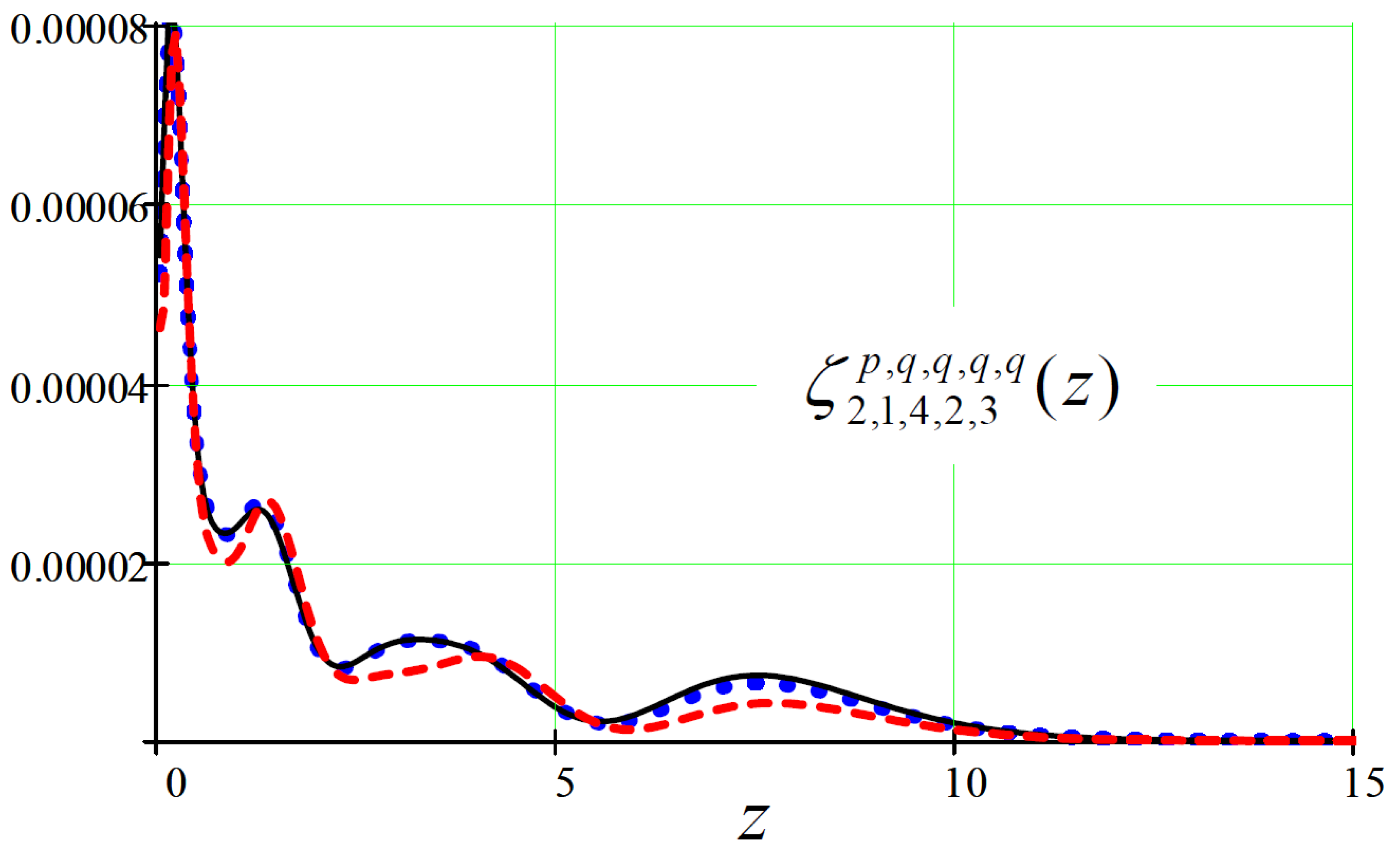
Figure 10.
Reproduction of Figure 9 (with a Gauss quadrature order of 60) but for 10 times the values of the indices demonstrating diminishing values (of the order of 200 times less) where we used the asymptotic formula (45) for the spectral polynomials.
Figure 10.
Reproduction of Figure 9 (with a Gauss quadrature order of 60) but for 10 times the values of the indices demonstrating diminishing values (of the order of 200 times less) where we used the asymptotic formula (45) for the spectral polynomials.
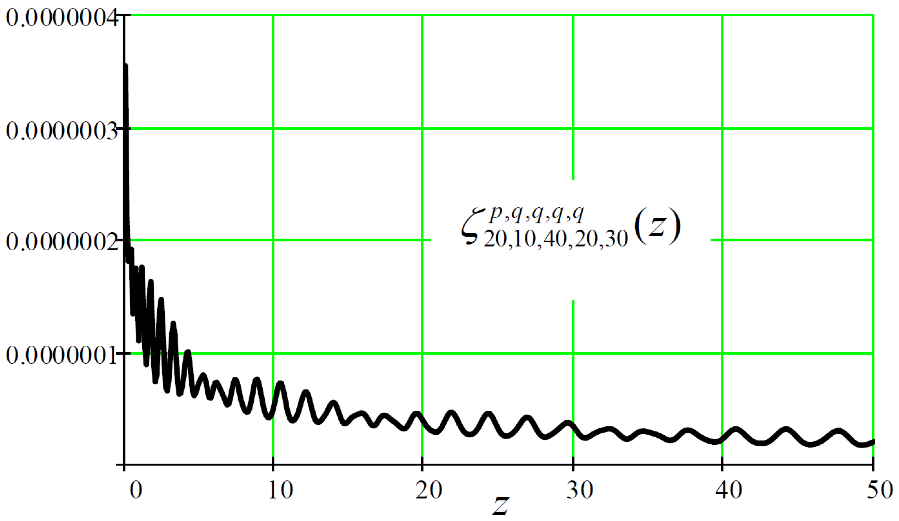
Figure 11.
Two-dimensional plot of the integral (46) viewed from two different angles. The x-axis scale is 0.15 while the y-axis scale is 0.30.
Figure 11.
Two-dimensional plot of the integral (46) viewed from two different angles. The x-axis scale is 0.15 while the y-axis scale is 0.30.
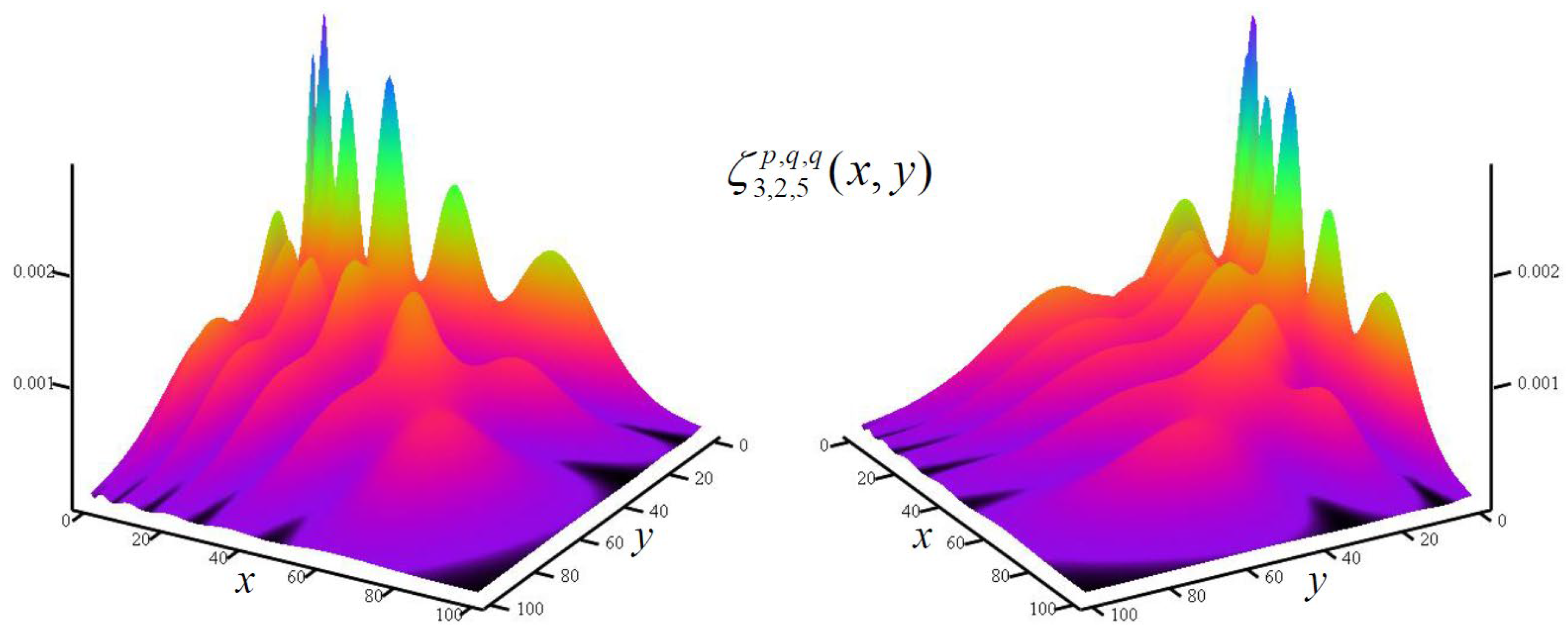

Table 1.
A list of for monochrome propagation and for several values of the energy and spinor parameter . In the formula (42), we took in calculating .
Table 1.
A list of for monochrome propagation and for several values of the energy and spinor parameter . In the formula (42), we took in calculating .
 |
Disclaimer/Publisher’s Note: The statements, opinions and data contained in all publications are solely those of the individual author(s) and contributor(s) and not of MDPI and/or the editor(s). MDPI and/or the editor(s) disclaim responsibility for any injury to people or property resulting from any ideas, methods, instructions or products referred to in the content. |
© 2025 by the authors. Licensee MDPI, Basel, Switzerland. This article is an open access article distributed under the terms and conditions of the Creative Commons Attribution (CC BY) license (http://creativecommons.org/licenses/by/4.0/).
Copyright: This open access article is published under a Creative Commons CC BY 4.0 license, which permit the free download, distribution, and reuse, provided that the author and preprint are cited in any reuse.


