Submitted:
17 March 2025
Posted:
17 March 2025
You are already at the latest version
Abstract
The increasing frequency and magnitude of flood-related disasters has led to adopting advanced flood models to provide a better understanding of flood vulnerability, particularly for human lives. Human flood vulnerability assessment is a primary objective when planning and designing in urban areas. Results of a numerical model in the coastal hamlet of Solanas (Sardinia, IT) in terms of water velocity and depth, have been processed using the empirical method of the regional legislation (RAS) as suggested by the National Network for the Environmental Protection. Vulnerability maps and statistical parameters were compared and benchmarked with the DEFRA method largely used in UK regarded as a state-of-the-art empirical approach. The main findings from the benchmark results between the DEFRA and RAS methods suggest that the applicability threshold of RAS method can significantly underestimate the pedestrian vulnerability to urban flood in Solanas and this paper suggests a preliminary step in improving that method could consider a tentative threshold value of 0.10 m depth to assure a more realistic evaluation of human vulnerability in Solanas.
Keywords:
urban flood
; numerical model
; MIKE+
; vulnerability index
; Sardinia
1. Introduction
Under climate change and urbanization, flood risk management has become a major issue for many urban areas [1]. Flood mapping is a central element of flood risk management [2], producing flood hazard maps which show the extent of flooded areas for various scenarios as requested by the European Flood Directive 2007/60. However, reliable flood mapping is difficult in small ungauged basins due to the lack of observed discharge data that are needed for calibrating the adopted hydrologic and hydraulic models. The primary methodology for estimating flood frequency would be fitting a theoretical statistical distribution to available measurements of flood peak discharges, but in the case of ungauged basins the most preferred approaches are the empirical and regional ones, since they do not require calibration. Conceptual models trying to represent in a simplified form the mechanisms governing the formation of the design hydrograph were developed in many scientific studies [3]. Recently, several simple conceptual rainfall-runoff models have been proposed [4].
In order to create a flood map, a hydrologic model must be combined with a hydraulic model. In recent decades, hydrodynamic modeling has been used to simulate flood dynamics, incorporating various levels of complexity, that range from 1D or 2D models to advanced, more rarely, 3D frameworks [5]. 1D models can be used for steady and unsteady flow analysis [6,7]. However, one disadvantage of 1D hydraulic models is that they do not provide information about the character and direction of the flow field or the way of flowing off the obstacles (such as buildings) which is most prominent in urban areas [8]. Although advanced 2D hydraulic approaches are more computationally expensive, requiring long processing times that limit their spatial and temporal scope [9], they are recommended for detailed local spatial scale areas and complex urban settings where the 1D hypothesis is often not applicable [10]. Most 2D hydrodynamic models (i.e., DELFT3D, HEC-RAS, MIKE21 and TELEMAC) use simplified versions of Navier-Stokes equations and principles of conservation of fluid mass and momentum on a grid that produce highly accurate flood simulations in urban areas [11]. Nevertheless, inherent large uncertainties, even in small basins, are present in multiple aspects of the hydrologic-hydraulic approaches involving the model structure, model parameters, boundary conditions or input data [12].
Urban open spaces are among the most vulnerable areas as they are where impacts are more acutely experienced [13]. Vulnerabilities include human life, sometimes disproportionately exposed in disadvantaged and marginalized communities [14], and building and infrastructure that do not tolerate exposure to rising and fast-moving flood waters [15]. In a future marked by populations concentrated in coastal cities [16] and significant trend in sea state parameters [17], the physical form of cities must be adaptive to flood events [18]. This includes the development and application of climate-resilient architectural design approaches [19] and the urban form of the community, including the density of development and the configuration of the street network and its relation to ground slopes which drive the movement of flood water [20].
This paper proposes a flood depth-velocity-damage function (FDVDF) fed by simulation results of MIKE+ 2D Overland [21] application in a small coastal urbanized basin in Southern Sardinia (Italy). Specifically, the FDVDF maps were used to evaluate the flood vulnerability in the hamlet of Solanas as a key indicator to support the plan and design of flood adaptation measures in urban public spaces. Furthermore, in this study an attempt is made to define how flood vulnerability index can support the selection of effective sustainable urban systems (SuDS) at the urban scales [22].
2. Materials and Methods
2.1. Mapping Urban Flood Vulnerability
The representation of the flooding phenomenon of the hamlet of Solanas uses the application of two-dimensional (2D) models in urban areas from the Article 8 of the Implementation Rules of the PAI introduced with the resolution of the Institutional Committee no. 1 of 27/02/2018. However, this study is not exhaustive with respect to the requirements of the Implementing Rules and develops only the aspects of greatest interest for some specific goals. The paragraph summarizes some aspects of the modeling and the main results useful for the enhancement of urban development and environmental enhancement of Solanas.
The development and application of modelling tools in the so-called residual basins defined as a part of territory not directly affected by the hydrographic network is having a growing interest. This modeling is different from that aimed at determining the hydraulic risk in the territories adjacent to the main hydrographic network where the water current associated with the flood with high return times (greater than 50 years) in the river network can often be represented by means of a linear hydraulic model (1D) to determine the average velocity and the water depth.
Modelling of the flood phenomenon in urban areas is distinguished by:
- Shorter return times (frequent and rapid phenomena);
- Different spatial representation (larger scale on limited map);
- The presence of obstacles and complex elevation trends do not allow a prevailing direction of flow.
The purpose of the modeling is to quantify the frequency of occurrence, intensity and magnitude of urban floods. Specifically, flood characteristics include flood depth, velocity and extent at specified return periods [25], that are mapped in the entire residual basin. Here, vulnerability is defined as the extent of harm to which the urban area is susceptible to floods to its exposure at a specific level of hazard. In general terms, exposure can include values such as people, property, economic activities, and cultural and natural heritages, located in hazard-prone areas. One of the fundamental aspects of flood risk management is to assess the vulnerability of inhabitants to floods in urban areas [26]. Human vulnerability is primarily related to the loss of life; non-fatal injuries (blunt trauma, contusions, lacerations and animal bites [27,28]) are considered. Anyway, it is to be noticed that flooding events resulting in non-fatal damages are seven times more likely to occur than those resulting in death [29]. Besides, sources of flood fatalities include pedestrian crossings, basement drownings, vehicular deaths, collapsed buildings, and electrocution [30]. Pedestrians walking in flooded urban areas is one of the major causes of death associated with flood events, as pedestrians tend to underestimate the impact that a flood flow can have on the human body [31]. Experimental activities showed that the predominant failure mechanism was sliding [32] and a good descriptor of the sliding mechanism is the product of depth (h) and velocity (v) [33,34]. To overcome the limitations of experimental activities involving people, [35,36] have proposed several conceptual modelling techniques on:
- toppling mechanism;
- complex velocity profile and forces acting on the human body;
- bed slope conditions;
- body shape characteristics;
- bias of controlled laboratory conditions.
[31] provided an extensive and rigorous investigation, comparison and benchmark of five methods (four used by government organizations, the fifth being regarded as a state-of-the-art empirical approach). In Italy, the guidelines of the National Network for the Environmental Protection (ISPRA) [37] indicate the conceptual method proposed by [38] and adopted by the Department for Environment, Food and Rural Affairs (DEFRA) to quantify the human vulnerability in UK in the following equation (1):
where h is in meters and v in meters per second, and DF is the debris factor whose value depends on the probability that debris would lead to a significantly greater vulnerability to pedestrians. Considering urban as the dominant land use, guidelines suggest:
if h < 0.25 m then DF = 0
otherwise DF = 1
The hydrogeological management plan (PAI) [39] in Sardinia significantly modified the ISPRA method both in the DF value and type of threshold. Specifically, RAS method assumes the mathematical form:
if h < 0.25 m then Vp = 0
otherwise Vp = h(v + 0.5) + 0.25
if Vp > 1 m then Vp = 1
The Municipalities can produce local studies with 2D modelling analysis for urban areas and identify those parts of the territory in which Vp assumes a value of less than or equal to 0.75 for all return periods (from 50 to 500 years) as critical areas (Hi*). In Hi* areas, no hazard mapping is required and no restrictions on land use are imposed.
2.2. Area of Study
Solanas is situated in the south-eastern area of Sardinia, IT, the second biggest island in the Mediterranean Sea. Solanas is the seaside hamlet of Sinnai whose geographical coordinates are approximately 39,3053° N latitude and 9,2045° E longitude. The administrative area of Solanas has an area of approximately 26.7 km2. The town of Solanas is located within a residual hydrographic basin (Figure 1), i.e. not characterized by a main hydrographic network. The surface area of this basin is equal to 1.3 km2, with an average altitude of 350 m on a range from mean sea level to an altitude of 550 m.
This residual basin is part of the main basin of Rio Solanas with an estimated length of 13.4 km and a drainage area of 34 km2. The Solanas basin shows mainly late Paleozoic plutonites and related phylonian complexes, some strips of Tertiary conglomerate deposits and extensive layers of Quaternary deposits. On a physiographic level, it is clear the greater importance of the piedmont valley sector, where the riverbed is not confined but it expands within a vast alluvial area. Along this stretch the stream shows a clear wandering attitude within robust terraced Holocene alluviums. The mouth is perennial with a tendency to open onto the Southeast edge of Solanas beach.
Solanas beach is of pocket beach type closed by two rocky headlands as limiting of the littoral cell with seaward the upper limit of the Posidonia oceanica meadow and morphostructures of the geological basement. The beach and coastal dunes at Solanas have always supplied sand for a wide range of uses, and initially the extracted volumes were limited to buckets, wheelbarrows, or small pickup truck loads. However, starting in the Post-World War II, and thanks to the urban development, the coastal and river sand has been extracted at an accelerated rate exceeding the natural replenishment rate of sand in this physiographic unit [23]. Due to the extractive character, this mining was an extremely pervasive and damaging activity that destroyed a large part of the coastal environment of Solanas. With an average available area by user of 9 m2/person, the physical carrying capacity [24] is equal to 4500 tourists in the summer season without considering eventually trends in sea state parameters.
Sardinian coastal areas have been subject to significant anthropogenic pressure and urbanization processes over the past 60 years. The urbanization of Solanas developed extremely rapidly from the 80’s to the end of last century (Figure 2). In 2004, the "save coasts" law was approved, which imposed as a safeguard measure the non-buildability of territories within two 2 kilometers from the shoreline. However, as the level of urbanization increases, the development of infrastructure has lagged considerably behind economic growth, particularly in the realm of urban drainage facilities, which have been inadequate and have resulted in frequent flooding events in Solanas in recent years.
2.3. Numerical Model Application to Solanas Flood
Referring to the scientific literature of the sector for further information, the methodology developed consists of two phases:
- Hydrological model of inflow-runoff transformation for the determination of runoff (net rainfall hyetogram with leak assessment) for reference rainfall events (gross rainfall from rainfall probability curves or historical rainfall grams);
- Hydraulic model for the study of surface current propagation by solving two-dimensional equations characterizing shallow water equation model – SWE – flow for underground and surface drainage.
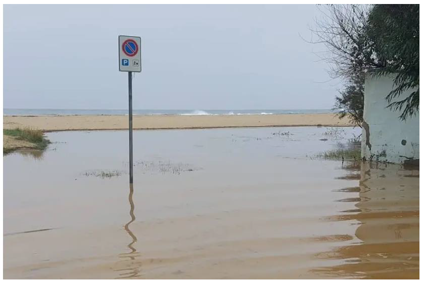
Figure 3.
Flooded area behind the dunal system of Solanas beach on 2nd February 2025. This area includes a large parking area (East side) and holiday houses (West side) (Source: Unione Sarda, newspaper).
Figure 3.
Flooded area behind the dunal system of Solanas beach on 2nd February 2025. This area includes a large parking area (East side) and holiday houses (West side) (Source: Unione Sarda, newspaper).
For the determination of the design hyetogram for the estimation of the flood hydrograph, please refer to the ADIS Guidelines (Guidelines and operational guidelines for the hydraulic modeling of flooding phenomena in residual urban basins) which indicate the use of a Chicago hyetogram for the cumulative precipitation height over any duration within the rainfall time for which the precipitation height is calculated with the rainfall probability curves for a return period of 25 years. Indication of the duration is provided by the time of concentration of the basin with the position of the peak equal to 0.4 of the duration.
The present study employs the MIKE+ hydrodynamic model [21] that offers a strong foundation for analyzing flood dynamics, especially in difficult terrains. MIKE+ 2D uses 2D modeling system that solves the two-dimensional St. Venant (dynamic flow) equations, using a cell-centered finite volume method. The time integration is performed using an explicit scheme and the numerical solution uses a self-adapting time step for optimizing stability and simulation times. The two-dimensional grid can be a normal rectangular grid or a mesh.
Specifically, MIKE+ 2D was used to simulate surface floods from surcharging collection system networks. Hydraulic model offers the most accurate and exhaustive approach in the description of the behavior of a fluid propagating on a locally complex topography (complex surface micro topography approach) such as the urban one in Solanas.
Model input data in the present study are:
In the Sardinia Region, residual basins are GIS elements contained in the latest update of the information layer of the Regional Geo-topographic database at 1:10.000 scale. From the identification of the catchment area and the hydrographic network, possibly residual with respect to the transformation carried out by urbanization, the model imports the DTM (Figure 5a) with the return of Figure 5b.
The numerical method used for the solution of the equations of the 2D problem uses the implicit finite volume algorithm that allows for larger time steps than explicit methods and an increase in stability compared to traditional finite difference or finite element methods. The solution of the analytical model takes place on an unstructured calculation mesh, represented in Figure 6a, on which the DTM of Figure 4 is interpolated returning the product of Figure 6b.
3. Results
Figure 6 and Figure 7 show the results of the numerical model in terms of the water depth and current velocity fields in the flooded portions (wet cells of the hydraulic model) from the surface runoff formed in the Solanas residual basin. The analysis allows to clearly identify the main characteristics of the urban flood. Comparing the fields of depth (h > 0.1 m) and velocity (v > 0.1 m/s), the latter is significantly wider (+72%) showing that a large part of flooded area has a current velocity with very low depth; in about half of these cells, the current velocity is higher than 0.5 m/s. The flood propagation is clearly defined along a NW-SE direction in two approximately parallel paths, the western in the urban area runs along the main street of Solanas hitting the buildings on both sides with a speed largely exceeding 1.5 m/s, and the eastern crossing a rural area with lower velocities (v < 0.5 m/s) and higher depth causes flooding in a depressed area of the countryside. Maximum values of depth and velocity in the entire residual basin are dmax = 0.97 m and vmax = 1.90 m/s. The rural area shows a higher flooding rate compared to the urban area, which may be attributed to differences in topography and drainage capacity, the latter mainly due to soil sealing from agricultural land use practices. Both flooding paths originate outside the urban area along deep incised canals that collect the outflows of the upstream portion of the basin. These flows cross the SP 17 at high speed where the drains of the artificial drainage network are undersized and poorly maintained. While these results enhance our understanding of flooding dynamics in Solanas, the complex patterns of depth and velocity need to be combined to properly develop targeted mitigation measures to reduce the vulnerability of future flooding events.
Flood Vulnerability Index Comparison
The results of the benchmark analysis for the RAS and DEFRA methods highlight the significant sensibility of the vulnerability predictions to model structure and parameters.
From the comparisons, it can be seen that the RAS model, rather than DEFRA model, produces is a significantly lower extension of the areas with an extreme FHR. The RAS model defines an application threshold of depth below which the vulnerability is not assessed. This is equivalent to establishing that pedestrians are not vulnerable to any flooding conditions when h < 0.25 m regardless of the velocity of the current. The portion of the residual basin in which this threshold is equaled or exceeded (area in Table 1) is equal to 14925 m2 or only 1.5% of the residual basin. On the contrary, the DEFRA model assesses the vulnerability throughout the flooded territory (area equal to 100% of the residual basin in Table 1). The DEFRA model uses the same depth value (h = 0.25 m) not as the threshold of applicability but as the threshold below which the probability that debris would lead to a significantly greater vulnerability to pedestrians is negligible. Therefore, for d < 0.25 m the debris factor is zero (DF = 0) (1). As a result, in the entire portion of the basin where the RAS model is applied, there is a vulnerability (A = AV = 14925 m2) against 70.9% by the DEFRA model. The second consequence concerns the statistics of the first (specifically the average vulnerability – AV – value) and the second order (the standard deviation – SDV – value). The applicability threshold of the RAS model (h = 0.25 m) results in a reduced map of 597 vulnerability values higher than the minimum value from equation (4) equal to 0.375 for h equal to the threshold and current velocity equal to zero (hydrostatic conditions of the current), as opposed to the DEFRA model which provides an extended map of 40804 vulnerability values where the minimum value is zero. This results in a greater dispersion of the vulnerability data sample in the DEDRA model (SDV = 0.15) than in the RAS model (SDV = 0.08), while the average vulnerability value of the RAS model is significantly higher (AV = 0.45) than in the DEFRA model (AV = 0.03). the maximum vulnerability value estimated by the DEFRA method (MV = 1.61) is significantly higher (+ 99%) than the value by the RAS method (MV = 0.81). This difference can be explained in part (76%) by the different coefficient of the two equations (DF = 1 for DEFRA, 0.25 for RAS) and in part (24%) by the different combination of d and v that maximizes vulnerability in the two methods. This last aspect highlights how RAS and DEFRA models, besides producing significantly different vulnerability values and their statistics, generate vulnerability maps with different spatial distributions, e.g., the urban area with maximum vulnerability from the two models is different.
The comparison between the spatial distributions of vulnerability values assumes a planning significance when associated with the following classes developed by [38,39] (Table 2). The RAS classification uses a threshold of Vp equal to 0.75 and the Municipalities shall introduce restriction on building rights only in those parts of the urban and peri-urban (Hi*) areas in which Vp is higher than 0.75 (high in Table 2). In the DEFRA classification 3 classes of vulnerability are defined above the Vp threshold of 0.75, each for a different group of people effectively at risk (i.e., for some – children –, for most, for all).
Figure 8 and Figure 9 clearly show that there are no significant urban and peri-urban areas with high vulnerability for the RAS method, while the DEFRA method shows areas of moderate and significant vulnerabilities in the terminal stretch of the two flood propagation paths along a NW-SE direction. In particular, while the RAS method does not highlight the need to introduce urban planning restrictions in Solanas, the DEFRA method identifies the roundabout of the main street (western path) and the depressed area of the countryside (eastern path) as project areas for vulnerability reduction interventions.

Table 2.
Vulnerability classification in DEFRA and RAS approaches.
| Vp | DEFRA class | RAS class |
|---|---|---|
| < 0.75 | low | low |
| 0.75 – 1.0 | moderate | high |
| 1.0 – 1.25 | ||
| 1.25 – 2.5 | significant | |
| > 2.5 | extreme |
4. Discussion
The comparison between the results of the two methods highlights the limitations of the RAS approach in representing the conditions of vulnerability of pedestrians in urban flooding conditions. The RAS method does not highlight significant portions of urban and peri-urban areas with vulnerability to depth and velocity for events with a return time of 25 years. In contrast, those conditions result in moderate and significant vulnerability in two areas of Solanas by the DEFRA method. Furthermore, these benchmark results confirm the caution needed in an empirical method alone [31]. While the authors acknowledge that rigorous validation and comparison of empirical methods is difficult to assess and largely beyond the scope of this paper, some of the inconsistencies between the different empirical methods are worthy of being used to support planning and design of flood mitigation measures in urban and peri-urban spaces such as Solanas. Both methods are based on the product of the depth and velocity and are largely inconsistent with an analysis of the hydrodynamic forces on a stationary body. This inconsistency is expected to be considerably high when the velocity is in excess of 1 m/s, as is generally the case for extreme flood events as that simulated in Solanas with a 25 year-return period.
As explained through the paper, the main difference in the predictions is thought to be due to the use of depth threshold. In both methods the threshold is set at 0.25 m. While in the RAS method it is a threshold of applicability of the method, in the DEFRA method it indicates the threshold below which the impact of debris flow in the conditions of pedestrian stability is negligible. The use of the RAS method applicability threshold indicates that below 0.25 m there is no pedestrian vulnerability. This aspect appears to be linked to the definition of vulnerability as the possibility of loss of human life due to slipping and consequent drowning but appears to be aimed at adult males in good physical condition. In reality, the DEFRA method indicates how fragile people (e.g., children, the elderly or people with reduced mobility) can lose their stability even in conditions of depth below the threshold. Details of forces acting on a flooded human body for sliding and toppling instabilities are provided by mechanics-based human behavior models [42].
The main findings from the benchmark results between the DEFRA and RAS methods suggest that the applicability threshold of RAS method can significantly underestimate the pedestrian vulnerability to urban flood in Solanas. While the definition of a new method is largely beyond the aim of this paper, a preliminary step in improving that method could consider a tentative threshold value of 0.10 m depth to assure a more realistic evaluation [42]. While preliminary, this step would allow to maintain the methodological approach referred to in the regional planning legislation in Sardinia (equations (2-5) and Table 2) but extending the vulnerability assessment to different combinations of depth and velocity in portions of the territory currently not under analysis.
Preserving the original methodological approach, in the entire portion of the basin where the modified RAS model (RAS_MOD) is applied, there is a vulnerability (A = AV = 97825 m2). The area in which conditions of vulnerability for the person arise increases significantly by 655%. Therefore, in the face of a substantial invariance of the values of maximum vulnerability and standard deviation, the average value of vulnerability decreases by about 27%. The fact that the area with vulnerability increases sixfold appears in Figure 10 where both NW-SE routes present vulnerabilities in a large part of their development while the terminal areas (the roundabout in the urban area and the depressed area in the peri-urban area) occupy significant portions of the territory defining those areas as unsafe for pedestrians.
Table 2.
Statistical summaries of vulnerability index comparison between RAS method and its modified version (RAS_MOD). Results highlight the RAS method sensibility to the d threshold (3) of zero vulnerability.
Table 2.
Statistical summaries of vulnerability index comparison between RAS method and its modified version (RAS_MOD). Results highlight the RAS method sensibility to the d threshold (3) of zero vulnerability.
| RAS | RAS_MOD | |
|---|---|---|
| Area [m2] | 14925 (1,5%) | 97825 (9,6%) |
| Area with vulnerability [m2] | 14925 (1,5%) | 97825 (9,6%) |
| Max Vulnerability | 0.81 | 0.81 |
| Std Dev Vulnerability | 0.08 | 0.09 |
| Average Vulnerability | 0.45 | 0.33 |
5. Conclusions
Although urban vulnerability highlights a complexity that the human component alone cannot describe, the assessment of the vulnerability of pedestrians to flooding in urban areas Although urban vulnerability highlights a complexity that the human component alone cannot describe, the assessment of the vulnerability of pedestrians to flooding in urban areas is a priority tool in urban center planning. In the case of Solanas, this vulnerability analysis can be an opportunity to rethink the public space capable of connecting and giving new order to individual settlement and agglomerations of second homes without a center. The two paths of the flood in urban and peri-urban areas require interventions in the form of SuDS (e.g., lamination park and permeable pavements) in a vision of adaptation to the natural phenomenon and urban redevelopment in which these interventions define new public spaces.
Funding
This research received no external funding.
Conflicts of Interest
The author declares no conflicts of interest.
References
- Degeai, J.-P.; Blanchemanche, P.; Tavenne, L.; Tillier, M.; Bohbot, H.; Devillers, B.; Dezileau, L. River flooding on the French Mediterranean coast and its relation to climate and land use change over the past two millennia. Catena 2022, 219, 106623. [Google Scholar] [CrossRef]
- Taillandier, F.; Taillandier, P.; Brueder, P.; Brosse, N. The dynamic sketch map to support reflection on urban flooding. International Journal of Disaster Risk Reduction 2025, 116, 105121. [Google Scholar] [CrossRef]
- Grimaldi, S.; Petroselli, A.; Serinaldi, F. A continuous simulation model for design-hydrograph estimation in small and ungauged watersheds. Hydrological Sciences Journal 2012, 57, 1035–1051. [Google Scholar] [CrossRef]
- Grimaldi, S.; Nardi, F.; Piscopia, R.; Petroselli, A.; Apollonio, C. Continuous hydrologic modelling for design simulation in small and ungauged basins: A step forward and some tests for its practical use. Journal of Hydrology 2021, 595, 125664. [Google Scholar] [CrossRef]
- Apel, H.; Aronica, G.T.; Kreibich, H.; Thieken, A.H. Flood risk analyses – how detailed do we need to be? Natural Hazards 2009, 49, 79–98. [Google Scholar] [CrossRef]
- Mark, O.; Weesakul, S.; Apirumanekul, C.; Aroonnet, S.B.; Djordjević, S. Potential and limitations of 1D modelling of urban flooding. Journal of Hydrology 2004, 299, 284–299. [Google Scholar] [CrossRef]
- Teng, J.; Jakeman, A.J.; Vaze, J.; Croke, B.F.W.; Dutta, D.; Kim, S. Flood inundation modelling: A review of methods, recent advances and uncertainty analysis. Environmental Modelling & Software 2017, 90, 201–216. [Google Scholar] [CrossRef]
- Horritt, M.S.; Bates, P.D. Evaluation of 1D and 2D numerical models for predicting river flood inundation. Journal of Hydrology 2002, 268, 87–99. [Google Scholar] [CrossRef]
- Fathi, M.M.; Liu, Z.; Fernandes, A.M.; Hren, M.T.; Terry, D.O.; Nataraj, C.; Smith, V. Spatiotemporal flood depth and velocity dynamics using a convolutional neural network within a sequential Deep-Learning framework. Environmental Modelling & Software 2025, 185, 106307. [Google Scholar] [CrossRef]
- Ignacio, J.A.F.; Cruz, G.T.; Nardi FHenry, S. Assessing the effectiveness of a social vulnerability index in predicting heterogeneity in the impacts of natural hazards: case study of the Tropical Storm Washi flood in the Philippines. Vienna Yearbook of Population Research 2015, 13, 91–129. [Google Scholar]
- Mudashiru, R.B.; Sabtu, N.; Abustan, I.; Balogun, W. Flood hazard mapping methods: A review. Journal of Hydrology 2021, 603, 126846. [Google Scholar] [CrossRef]
- Dimitriadis, P.; Tegos, A.; Oikonomou, A.; Pagana, V.; Koukouvinos, A.; Mamassis, N.; Koutsoyiannis, D.; Efstratiadis, A. Comparative evaluation of 1D and quasi-2D hydraulic models based on benchmark and real-world applications for uncertainty assessment in flood mapping. Journal of Hydrology 2016, 534, 478–492. [Google Scholar] [CrossRef]
- Intergovernmental Panel on Climate Change. Managing the Risks of Extreme Events and Disasters to Advance Climate Change Adaptation; Cambridge University Press: Cambridge, UK; New York, NY, USA, 2012. [Google Scholar]
- Rufat, S.; Tate, E.; Burton, C.G.; Maroof, A.S. Social vulnerability to floods: Review of case studies and implications for measurement. Int. J. Disaster Risk Reduct. 2015, 14, 470–486. [Google Scholar] [CrossRef]
- Wing, O.E.; Pinter, N.; Bates, P.D.; Kousky, C. New insights into us flood vulnerability revealed from flood insurance big data. Nat. Commun. 2020, 11, 1444. [Google Scholar] [CrossRef] [PubMed]
- Cosby, A.G.; Lebakula, V.; Smith, C.N.; et al. Accelerating growth of human coastal populations at the global and continent levels: 2000–2018. Sci Rep 2024, 14, 22489. [Google Scholar] [CrossRef]
- Ardhuin, F.; Stopa, J.E.; Chapron, B.; Collard, F.; Husson, R.; Jensen, R.E.; Johannessen, J.; Mouche, A.; Passaro, M.; Quartly, G.D.; Swail, V.; Young, I. Observing Sea States. Frontiers in Marine Science 2019, 6. [Google Scholar] [CrossRef]
- Matos Silva, M.; Costa, J.P. Flood Adaptation Measures Applicable in the Design of Urban Public Spaces: Proposal for a Conceptual Framework. Water 2016, 8, 284. [Google Scholar] [CrossRef]
- Watson, D.; Adams, M. Design For Flooding: Architecture, Landscape, And Urban Design For Resilience To Climate Change. John Wiley & Sons, 2020. [Google Scholar]
- Balaian, S.K.; Sanders, B.F.; Abdolhosseini Qomi, M.J. How urban form impacts flooding. Nat Commun 2024, 15, 6911. [Google Scholar] [CrossRef]
- MIKE + 2D Manual (2023). User Manual. DHI Technical Report.
- Sulis, A.; Altana, M.; Sanna, G. Assessing Reliability, Resilience and Vulnerability of Water Supply from SuDS. Sustainability 2024, 16, 5391. [Google Scholar] [CrossRef]
- Programma Azione Coste della Sardegna, 2013. Regione Autonoma della Sardegna. Technical Report. https://www.regione.sardegna.it/documenti/1_274_20140121114459.pdf.
- Sulis, A.; Carboni, A.; Manca, G.; Yezza, O.; Serreli, S. Impacts of climate change on the tourist-carrying capacity at La Playa beach (Sardinia, IT). Estuarine, Coastal and Shelf Science 2023, 284, 108284. [Google Scholar] [CrossRef]
- UNDRR, 2020. Human Cost of Disasters, Human Cost of Disasters. An overview of the last 20 years 2000-2019. [CrossRef]
- Arrighi, C.; Pregnolato, M.; Dawson, R.J.; Castelli, F. Preparedness against mobility disruption by floods. Sci. Total Environ. 2019, 654, 1010–1022. [Google Scholar] [CrossRef]
- Vinet, F. (Ed.) Flood Impacts on Loss of Life and Human Health. In Floods; Elsevier, 2017; pp. 33–51. [Google Scholar] [CrossRef]
- Yari, A.; Ostadtaghizadeh, A.; Ardalan, A.; et al. Risk factors of death from flood: Findings of a systematic review. J Environ Health Sci Engineer 2020, 18, 1643–1653. [Google Scholar] [CrossRef]
- Kaiser, M.; Günnemann, S.; Disse, M. Spatiotemporal analysis of heavy rain-induced flood occurrences in Germany using a novel event database approach. Journal of Hydrology 2021, 595, 125985. [Google Scholar] [CrossRef]
- Agonafir, C.; Lakhankar, T.; Khanbilvardi, R.; Krakauer, N.; Radell, D.; Devineni, N. A review of recent advances in urban flood research. Water Security 2023, 19, 100141. [Google Scholar] [CrossRef]
- Musolino, G.; Ahmadian, R.; Falconer, R.A. Comparison of flood hazard assessment criteria for pedestrians with a refined mechanics-based method. Journal of Hydrology X 2020, 9, 100067. [Google Scholar] [CrossRef]
- Foster, D.N.; Cox, R. Stability of children on roads used as floodways: preliminary study. 1973; 12. [Google Scholar]
- Abt, S.R.; Wittier, R.J.; Taylor, A.; Love, D.J. Human stability in a high flood hazard zone. J. Am. Water Resour. Assoc. 1989, 25, 881–890. [Google Scholar] [CrossRef]
- Jonkman, S.N.; Penning-Rowsell, E. Human Instability in Flood Flows. JAWRA Journal of the American Water Resources Association 2008, 44, 1208–1218. [Google Scholar] [CrossRef]
- Jonkman, S.N.; Penning-Rowsell, E. Human Instability in Flood Flows1. JAWRA Journal of the American Water Resources Association 2008, 44, 1208–1218. [Google Scholar] [CrossRef]
- Chen, Q.; Xia, J.; Falconer, R.A.; Guo, P. Further improvement in a criterion for human stability in floodwaters. J Flood Risk Management 2019, 12, e12486. [Google Scholar] [CrossRef]
- Ramsbottom, D.; Wade, S.; Bain, V.; Hassan, M.; Penning-Rowsell, E.; WIlson, T.; Fernandez, A.; House, M.; Floyd, P. Flood Risk to People: Phase 2. R&D Technical Report FD, Department for the Environment, Food and Rural Affairs (DEFRA), UK Environment Agency. 2016. [Google Scholar] [CrossRef]
- Istituto Superiore per la Protezione e la Ricerca Ambientale. Proposta metodologica per l’aggiornamento delle mappe di pericolosità e di rischio, Proposta metodologica per l'aggiornamento delle mappe di pericolosità e di rischio. 2012.
- Piano Stralcio Assetto Idrogeologico (PAI) della Sardegna. Norme Tecniche di Attuazione. Update to 21.11.2024. Norme di Attuazione al PAI - Autorità di Bacino.
- Cox, R.J.; Shand, T.D.; Blacka, M.J. Australian rainfall and runoff (AR&R). Revision project 10: appropriate safety criteria for people. 2010. [Google Scholar]
- Martínez-Gomariz, E.; Gómez, M.; Russo, B. Experimental study of the stability of pedestrians exposed to urban pluvial flooding. Nat Hazards 2016, 82, 1259–1278. [Google Scholar] [CrossRef]
- Li, Q.; Xia, J.; Dong, B.; Liu, Y.; Wang, X. Risk assessment of individuals exposed to urban floods. International Journal of Disaster Risk Reduction 2023, 88, 103599. [Google Scholar] [CrossRef]
Figure 1.
Geographic location of the study area, buildings are in red; detail of hydrographic basin with urbanized area of Solanas.
Figure 1.
Geographic location of the study area, buildings are in red; detail of hydrographic basin with urbanized area of Solanas.
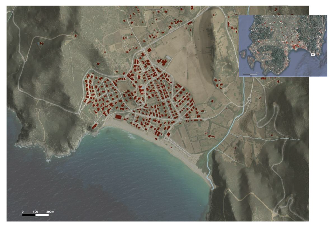
Figure 2.
Orthophoto timeseries of the urbanixed area of Solanas: 1968 (upper left), 1977 (upper right), 2006 (lower left), 2019 (lower right).
Figure 2.
Orthophoto timeseries of the urbanixed area of Solanas: 1968 (upper left), 1977 (upper right), 2006 (lower left), 2019 (lower right).
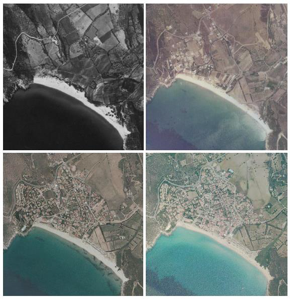
Figure 4.
Buildings (grey) and road network (orange) in the residual basin of Solanas. Limits are green. DTM at 1 m spatial resolution.
Figure 4.
Buildings (grey) and road network (orange) in the residual basin of Solanas. Limits are green. DTM at 1 m spatial resolution.
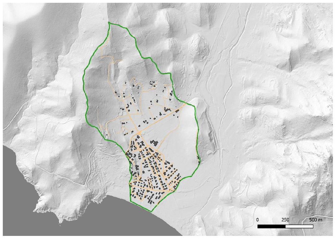
Figure 5.
Construction of modelling dataset (a) DTM in the residual basin of Solanas; (b) Imported DTM in MIKE+ User Interface.
Figure 5.
Construction of modelling dataset (a) DTM in the residual basin of Solanas; (b) Imported DTM in MIKE+ User Interface.
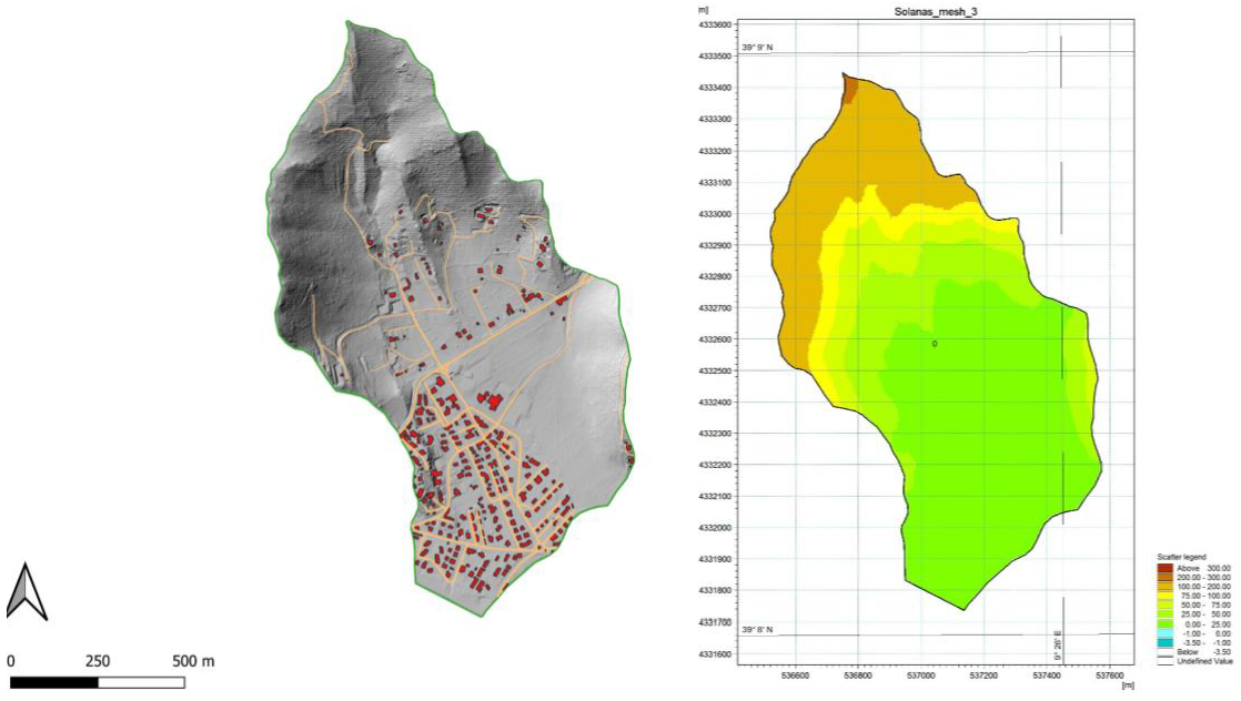
Figure 6.
Construction of modelling dataset (a) Triangular adaptive flexible mesh; (b) Discretized DTM in the adopted grid.
Figure 6.
Construction of modelling dataset (a) Triangular adaptive flexible mesh; (b) Discretized DTM in the adopted grid.
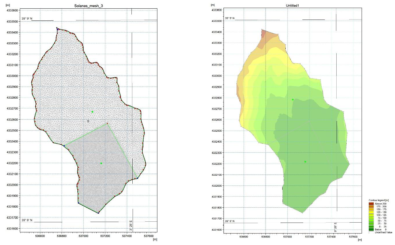
Figure 6.
Flood depth map.
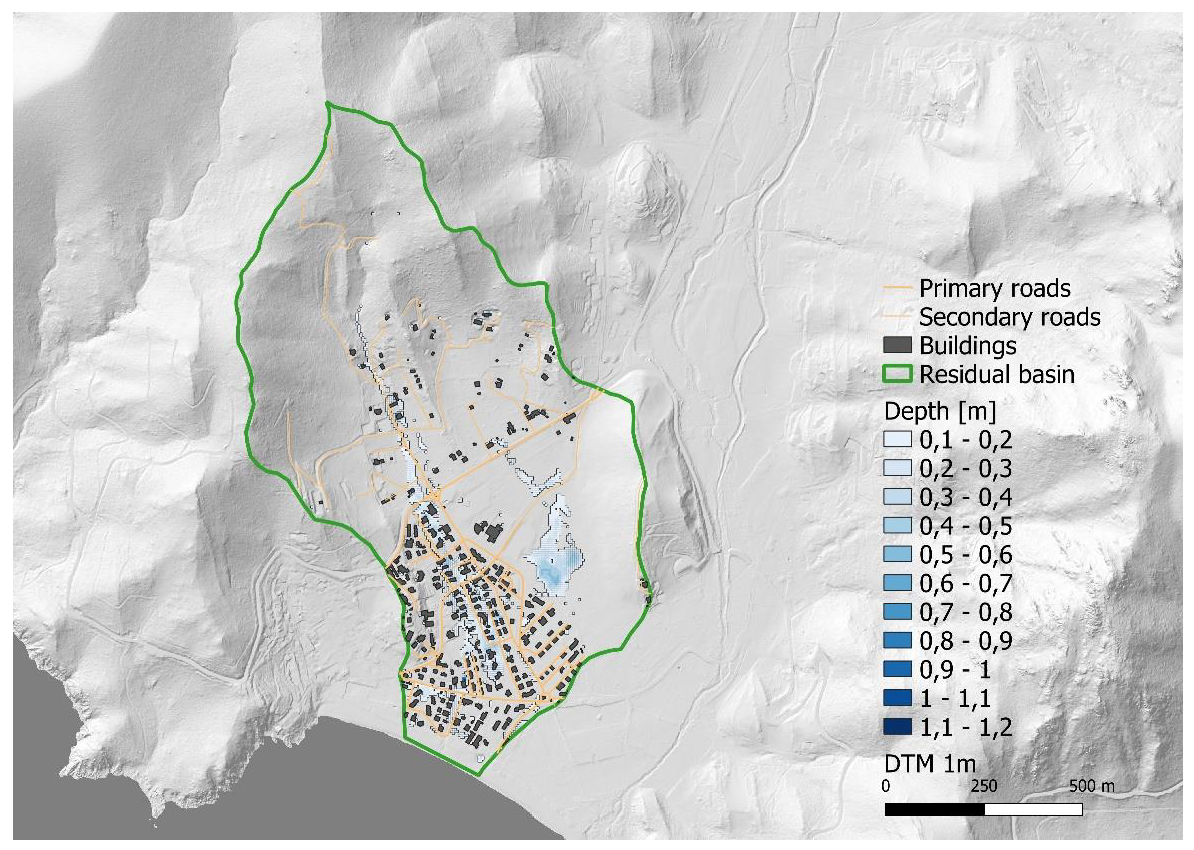
Figure 7.
Current velocity map.
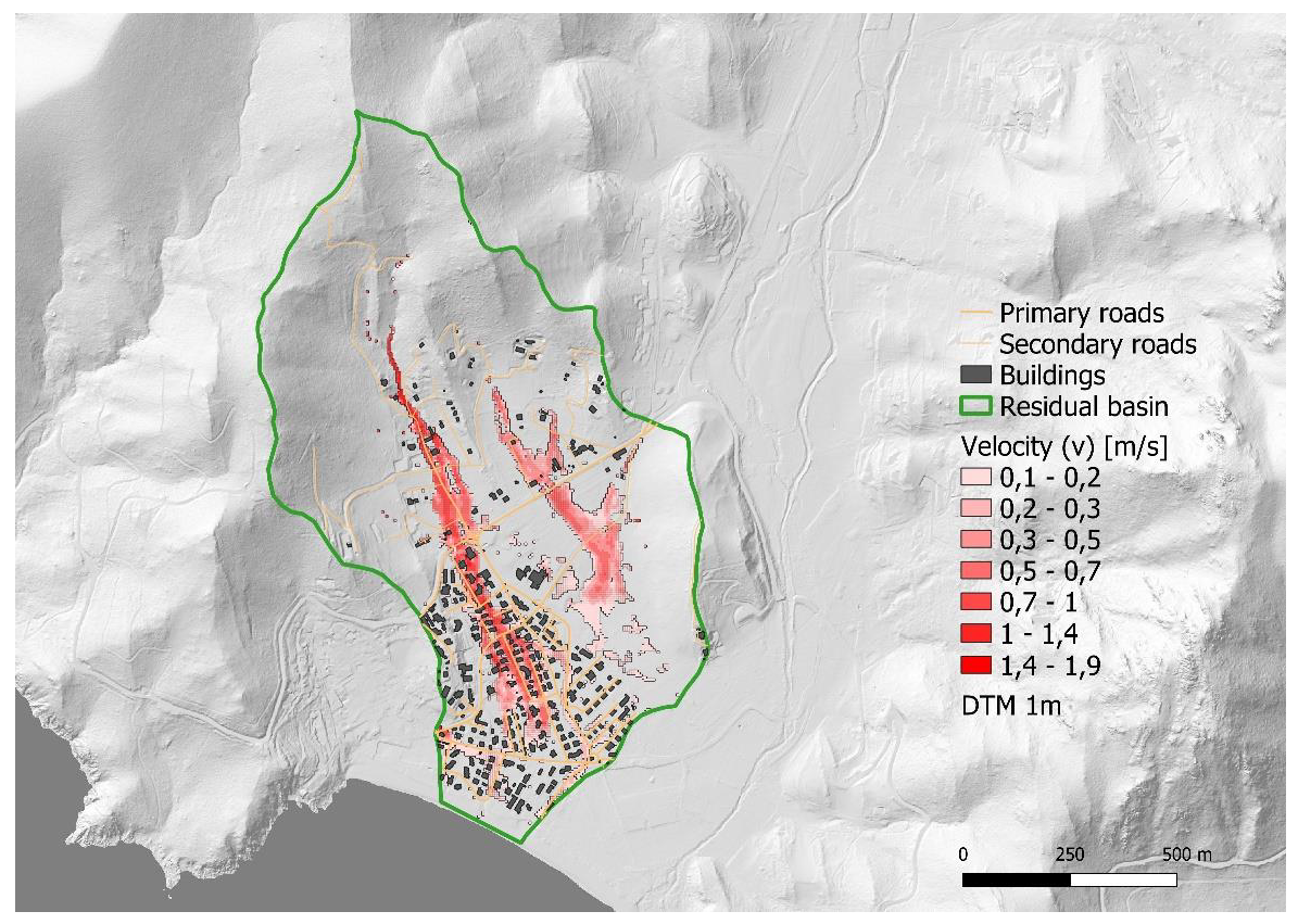
Figure 8.
RAS vulnerability map where two classes are shown in the residual basin of Solanas, i.e. the low vulnerability in yellow and the high vulnerability in red (few and disconnected cells of 5 x 5 m).
Figure 8.
RAS vulnerability map where two classes are shown in the residual basin of Solanas, i.e. the low vulnerability in yellow and the high vulnerability in red (few and disconnected cells of 5 x 5 m).
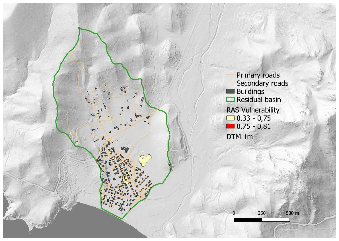
Figure 9.
DEFRA vulnerability map where three classes are shown in the residual basin of Solanas, i.e. the low vulnerability in green, the moderate vulnerability in light red and the significant vulnerability in dark red (only small cell of 5 x 5 m).
Figure 9.
DEFRA vulnerability map where three classes are shown in the residual basin of Solanas, i.e. the low vulnerability in green, the moderate vulnerability in light red and the significant vulnerability in dark red (only small cell of 5 x 5 m).
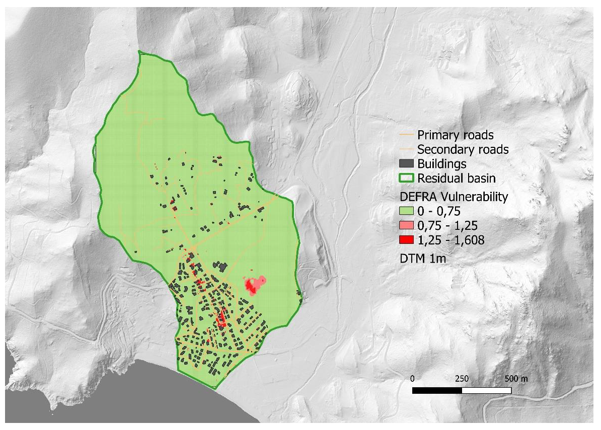
Figure 10.
RAS_MOD vulnerability map with a depth threshold of 0.10 m.
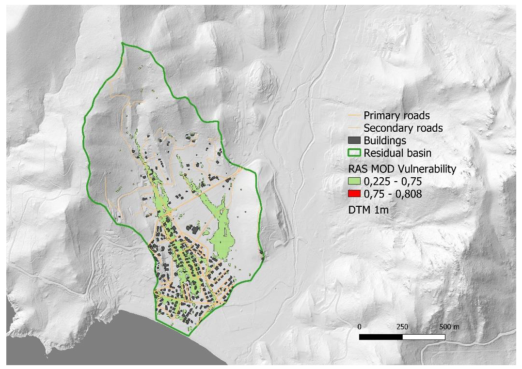
Table 1.
Statistical summaries of vulnerability index comparison between RAS and DEFRA methods. Area is the extension of territory where the indicator is evaluated being water depth above the predefined threshold; vulnerable area is the extension of territory where vulnerability indicator is different from zero; statistical indicators (max, average, standard deviation – std dev) are calculated in the area with vulnerability.
| RAS | DEFRA | |
|---|---|---|
| Area [m2] (A) | 14925 (1,5%) | 1020100 (100%) |
| Vulnerable Area [m2] (AV) | 14925 (1,5%) | 723475 (70,9%) |
| Max Vulnerability (MV) | 0.81 | 1.61 |
| Std Dev Vulnerability (SDV) | 0.08 | 0.15 |
| Average Vulnerability (AV) | 0.45 | 0.03 |
Disclaimer/Publisher’s Note: The statements, opinions and data contained in all publications are solely those of the individual author(s) and contributor(s) and not of MDPI and/or the editor(s). MDPI and/or the editor(s) disclaim responsibility for any injury to people or property resulting from any ideas, methods, instructions or products referred to in the content. |
© 2025 by the authors. Licensee MDPI, Basel, Switzerland. This article is an open access article distributed under the terms and conditions of the Creative Commons Attribution (CC BY) license (http://creativecommons.org/licenses/by/4.0/).
Copyright: This open access article is published under a Creative Commons CC BY 4.0 license, which permit the free download, distribution, and reuse, provided that the author and preprint are cited in any reuse.


