Challenges and Opportunities in ILR Selection for Photovoltaic System: Evaluation in Brazilian Capitals

1. Introduction

Addressing performance evaluation before and after designing on-grid PV systems ensures PV installation's efficiency, reliability, and effectiveness. In a macro scenario, it guides policy decisions and financial investments, and at a component level, it helps identify potential areas for improvement and optimize the energy output.

Brazil's Federal Law 14300/2022 reduced the subsidies in the distributed energy net-metering policy implemented in the Normative Resolution nº 482/2012; this last one allowed fast growth in the distributed solar PV sector [1,2]. In contrast, residential electricity rates have kept rising since 2019, and the PV system cost has lowered, maintaining optimistic future scenarios [1].

Intermittent energy sources like solar and wind power make it difficult to evaluate performance because they directly affect energy production. PV plants are also affected by the array strategy, azimuth, and inclination. When solar irradiance on the plane decreases, and the ambient temperature rises for extended periods, the energy output of PV generators is negatively impacted. As a result, the inverter, with nonlinear losses, may operate at low efficiency, leading to increased losses. The designed relationship between the inverter's nominal power and the generator may help mitigate these losses.

The Inverter Load Ratio (ILR) is a crucial factor in determining the sizing of on-grid PV plants, as highlighted in the literature. Old references usually evaluate the ratio between the inverter's nominal power and the total array output power at the maximum power point under Standard Test Conditions; the ILR is the inverse. Once the interpretation of the results is the same, only the ILR acronym is used in this work.

It is common practice to install a larger PV generator than the inverter's nominal power (ILR>1); this feature allows the generator to maintain maximum power output for extended periods on sunny days and increases power production in low-light conditions, leading to greater overall energy generation. From a cost perspective, adding PV modules is more cost-effective than designing a new inverter. Oversizing the PV system compared to the inverter's nominal power does not shut down the system if the current and voltage input are below the inverter limits. Instead, it only restricts the injected power. This necessitates precise daylight data, a deep understanding of the inverter's efficiency-power characteristics, and the inverter's capability to promptly and permanently limit power without any interruption or damage [3,4].

The inverter's temperature increases after prolonged operation at maximum power and is also affected by the ambient temperature. By design, additional measures are taken to maintain the temperature within permissible limits, resulting in significant power losses as it prevents reaching the rated AC power [3,4]. Generally, the output power linearly decreases after reaching a temperature setpoint; this behavior varies by manufacturer. Conversely, using an inverter that's too large (ILR>1) results in low efficiency at average and low levels of sunlight, which increases costs and reduces financial viability [5].

Studies [6,7] demonstrate that the thermal stress in the solar inverter components reduces its lifetime. They indicate that lower annual irradiation and ambient temperature contribute to longer inverter lifetimes [6,7]. High irradiation and temperature levels lead to extended operation in power-limiting mode, resulting in higher thermal loading and reduced lifetime due to its effect on power devices (IGBTs) and DC-link components like capacitors [6,7]. Conversely, increasing ILR has a lesser impact on lifetime in areas with high annual irradiation [6,7]. For example, increasing ILR from 1.0 to 1.4 in Arizona resulted in a 22% reduction in lifetime, while further increases had a minimal effect [6]. This research leverages areas with high yearly irradiation levels, assuming the system will require only one replacement inverter over its lifetime. Future studies could investigate different replacement schedules based on new discoveries.

The [8] review concludes that in the industry, extensive testing is done on individual components to calculate their failure-rate distribution, which is then used to predict performance under actual usage conditions. However, assessing the reliability of assembled components in power conditioning equipment within a complex environment is challenging [8]. This challenge becomes increasingly complex as the capacity rating of the inverter grows, incorporating a greater number of components [8]. Existing literature evaluates key parameters such as ambient temperature and irradiation [6,7]. However, a comprehensive evaluation should also consider factors such as the impact of the temperature and the moisture ingress on the device and the presence of acids in solder flux, soiling, and pollution, which can accelerate temperature and humidity-related degradation mechanisms [8].

The conditioned power and DC voltage influence a grid-connected inverter's efficiency [9-11]. For this last one, there is no general rule or model; it depends on the manufacturer's design, and they provide at least three efficiency curves for different voltages. The inverter's efficiency in relation to its load and DC input voltage has been the subject of various proposed analytical expressions, as highlighted in the work by [11].

In PV sizing design, the minimum and maximum number of series-connected PV modules per string must be known to allow the inverter to start, avoid damage, and operate in the maximum power point tracker (MPPT) voltage range. [9] created a model to determine these limits based on the inverter and PV module voltages, PV cell temperature, and irradiance. To maximize annual inverter efficiency, [9] suggests maximizing the number of series-connected PV modules per string without surpassing the inverter's voltage limits and increasing the ILR towards the right of the optimal annual efficiency point until the efficiency value decreases by 0.1%.

Despite the DC voltage influence, studies have revealed variations in maximum efficiency of approximately 3% for transformerless inverters [10,12], which is minimal, less than 1%, for inverters with maximum efficiency equal to or exceeding 97% [10]. Therefore, the ILR significantly impacts the yearly DC/AC conversion efficiency more than the array-to-inverter voltage sizing ratio [9]. Thus, this work utilizes only the medium efficiency curve.

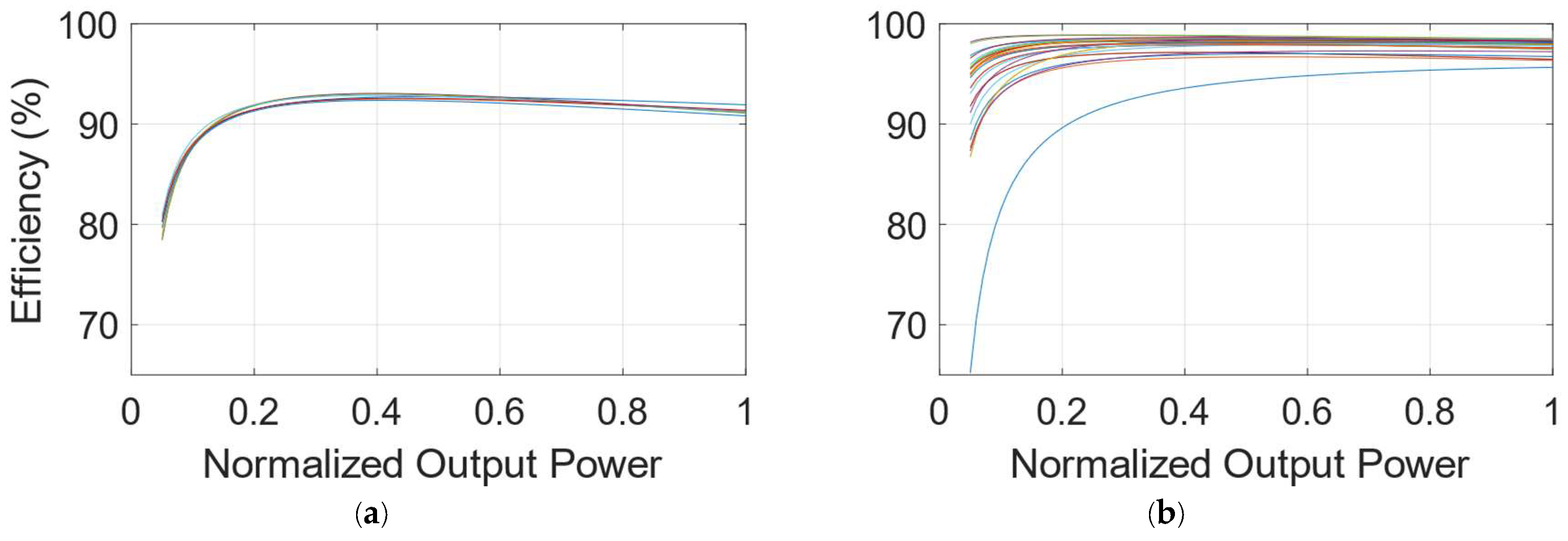
Although not a comprehensive comparison, when we compare the normalized efficiency curves of eight commercialized inverters in Brazil in 2007 [4] with the 28 commercial inverters discussed in this paper, it becomes evident that there have been significant technological advancements (Figure 1). Twenty-seven inverters in this study exhibit higher efficiency than those in 2007, with the remaining inverter incorporating older low-efficiency technology. The increase is particularly noticeable for high-power inverters, which maintain high efficiency even under low-power conditions.

The inverter's nonlinear behavior and its cost impact on the system are the main reasons for seeking its optimal ILR. However, before worrying about it, the PV generator must be optimized regarding cabling, direction, horizontal inclination, and PV technology, mainly constrained in lower power plants with fixed direction and roof inclination.

This study introduces a range of ILR values that result in minimal energy losses and LCOE. The goal is to optimize and analyze the sizing process for various inverter technologies and power outputs ranging from 3 to 120 kW, suitable for both small and large-scale grid-connected solar photovoltaic (PV) systems. The study encompasses 27 cities in Brazil with annual radiation levels between 1522 and 2225 kWh/m².

The paper is organized as follows:

• Section II provides background information on analyzing the optimal Inverter Load Ratio (ILR) and sizing grid-connected PV systems, focusing on works considering Final Yield and Levelized Cost of Energy (LCOE);
• Section III describes the simulation methods used, including generation modeling, electrical parameters of inverters and modules, loss accounting, and financial modeling for PV plants in the Brazilian Market;
• Section IV discusses solar resources in Brazilian capitals, critically analyzes clipping losses and inverter efficiency considering the aging losses, and evaluates the optimal ILR within the range of 0.8 to 2.0 (120 ILRs) and their impact on Final Yield and LCOE for 27 Brazilian capitals and 28 commercial inverters;

Finally, Section V presents the conclusions of the study.

2. Background Literature Research

Exploring the optimum Final Yield and its relationship to the ILR, [5,13] found that the optimum ILR, which maximizes the Final Yield, is a function of the local climate. It is typically from about 1 for high insolation conditions to well above 2 for low insolation values. However, given its orientation and thermal effects, those values must consider the actual PV array output [5,14].

Over a year, a 5-minute monitored experiment was conducted in São Paulo, Brazil, involving eight ILRs ranging from 0.98 to 1.82 [4]. The main parameters measured were incident irradiance, temperature, PV generator output, inverter output, and the Final Yield. The study confirmed that the relative capacity of the inverter compared to the PV generator under tests did not significantly affect the Final Yield, remaining the at or below 100 kWh/kWp in 2004. That aspect provides much freedom in the design stage.

Previous research [3,5,14] found that optimizing the ILR based on investment cost, specifically the ratio of photovoltaic (PV) to inverter cost [15], is more cost-effective than focusing on specific energy output or inverter efficiency. This approach often results in a higher ILR for inverters with high efficiency at low input power [15]. In a high-efficiency inverter system, the sizing of PV and inverter is more flexible than in a low-efficiency inverter system, which is typical of modern inverters [3,15].

When examining the utilization of multiple MPPTs, [16] observed that systems divided among various orientations result in less energy clipping than systems oriented in a single direction. Nevertheless, this approach is a means to restrict the input power of the inverter. When considering the high efficiencies of modern MPPTs and DC/AC conversion, it is crucial to assess whether this approach increases overall generator costs. Although this strategy reduces the amount of clipped energy, it can also lead to a reduction in generation.

[17] uses the optimal ILR range strategy to determine the size of PV systems. Their methodology involves finding the intersection region of three optimal sizing ranges based on three parameters: AC annual energy output (Eac, in kWh) and two economic criteria (in kWh/€). Each optimal range is the +/- 1% variation of the ILR that maximizes each parameter. Their main finding is that when factoring in a 1% annual degradation of the PV modules over a 20-year lifespan, the optimal ILR ranges increase by 10% compared to those that do not account for degradation. The degradation reduces the power output of the PV system, resulting in less clipped energy in the inverter. According to [16], the estimated total clipped energy over a 25-year lifetime was 5.1%.

Overload protection delay time has been simulated for up to 5 minutes to account for potential energy gain during the overload [18,19]. This means that when the inverter overloads, the input power is not immediately clipped. Brief spikes are allowed to pass through if they last less than the specified delay period. During an overload condition, the inverter's efficiency decreases as the load increases, and it may drop to 65% of efficiency at 150% of the nominal load [18,19]. This means that even with decreased efficiency, some energy loss due to high irradiance can be recycled and factored into the ILR choice [18,19]. In sunny areas, overload events tend to last longer without fluctuation, which causes the inverter to remain in protection mode because it does not have enough time to cool down, thus maintaining the clipping [18,19].

This results in a lack of new energy gains during the overload, making the resulting gain less significant than in less sunny areas. To analyze the delay requires high-resolution meteorological data, with at least one-minute sampling intervals, which differs from the commonly available hourly-based open-access data. Most provide historical averages, which may suppress irradiance spikes that exceed the inverter's maximum load. Furthermore, inverter manufacturers should provide information about this delay and the efficiency behavior during overload conditions. Hence, this study does not consider the delay in the protection system.

A methodology was developed in [20] to estimate optimal inverter sizing in Bahia, Brazil, considering overload losses and economic aspects. The study applied the methodology to five PV technologies (a-Si/µc-Si, a-Si, CIGS, c-Si, and m-Si) using one year of measured irradiance and temperature data. The generators used a 2.5 kW inverter with each PV technology, with the highest being 2.3 kWp to prevent clipping. The measured output power values are extrapolated linearly to the larger ILR. The difference is considered the overload loss if an extrapolated value exceeds the inverter's maximum output. The study proposes that the optimum ILR can be determined by calculating the maximum value of the ratio between marginal energy gain and marginal cost increase for different overloading of the PV inverter.

The results showed that the optimum ILR for commonly employed PV technologies like c-Si and m-Si is between 121% and 130%, depending on the DC cost ratio, with a representative ILR of 126%. The study also identified factors impacting the performance of different PV technologies, such as initial degradation, soiling, spectral response, weak-light response, and temperature losses in PV modules. Therefore, the approach of [20] hinges on precise on-site measurements using an oversized inverter, ensuring an ILR > 0.82 to avoid clipping and effectively represent the DC/AC losses in the extrapolated results. Furthermore, this methodology may lack commercial feasibility as it necessitates the evaluation of numerous equipment during the design phase.

The literature review reveals that many studies overlook the impact of degradation on photovoltaic (PV) lifetime when assessing the ILR or do not go deeper into their impact on the choice of ILR. On the other hand, this study examines the resultant DC loss curve in relation to ILR, how it evolves over time, and its influence on efficiency and Final Yield. The approach utilized in this research can be reproduced in diverse locations and adapted to different kinds of inverters, solar technologies, and economic contexts. It provides a thorough method for designing on-grid PV systems when evaluating various inverters and cities for the solar power plant.

Economic policies related to net metering, government subsidies, and electricity rates vary by country and depend on the type of electricity market for the PV plant (regulated or deregulated/competitive). This work does not address these policies to simplify the analysis and concentrate on other objectives.

3. Methodology

3.1. Generation Modeling

The computer simulations used hourly irradiance and temperature data from the 27 Brazilian state capitals [21]. For all cities (Table 1), the irradiance data on the generator plane are relative to the slope equal to the location's latitude with the generator facing north.

Since the inverters have the maximum power point tracking function, the maximum power ($P_m$) supplied by the generator can be determined through (1) where, in addition to the instantaneous irradiance in the generator plane ($H_{t,\beta }$) the effect of the temperature of the PV modules (2) is also accounted for as [22,23,24]:

$$P_m=P_{m,ref}·{\displaystyle \frac{H_{t,\beta }}{H_{ref}}}\left[1+\gamma \left(T_c-T_{c,ref}\right)\right],$$

(1)

$$T_c=T_a+{\displaystyle \frac{H_{t,\beta }}{800}}\left(NOCT-20\right)·0.9.$$

(2)

$P_{m,ref}$ is the maximum power of the generator in the STC (Standard Test Conditions: irradiance of 1,000 W/m², cell temperature of 25 °C ($T_{c,ref}$) and Air Mass of 1.5), $T_a$ is the ambient temperature, NOCT is the nominal operating temperature of the cell under irradiance of 800 W/m², and $\gamma$ is the temperature coefficient of the maximum power point.

Twenty-eight inverters from six manufacturers (Fronius, ABB, SMA, Refusol, Hauweii, and Canadian), each combined with one type of PV module (Table 2), were simulated. The nominal power ranges from 3 to 120 kW (Table 3).

The inverter efficiency (3), in general, depends on the output power and can be expressed in terms of losses due to self-consumption (k0), voltage drop (k1), and ohmic losses (k2) as [25,26]

$${\eta }_{Inv}={\displaystyle \frac{p_{out}}{p_{out}+k_0+{k_1·p}_{out}+k_2·p_{out}^2}},$$

(3)

where the power ratings of the inverters normalize the instantaneous AC output power ($p_{out}$), and the denominator accounts for the normalized instantaneous DC input power. The parameters of losses (4), (5), and (6) can be obtained through efficiencies in 10%, 50%, and 100% (${\eta }_{10\mathrm{\%}}$, ${\eta }_{50\mathrm{\%}}$, and ${\eta }_{100\mathrm{\%}}$ respectively) of the rated inverters AC power [27]:

$$k_0={\displaystyle \frac{1}{9}}·{\displaystyle \frac{1}{{\eta }_{100\mathrm{\%}}}}-{\displaystyle \frac{1}{4}}·{\displaystyle \frac{1}{{\eta }_{50\mathrm{\%}}}}+{\displaystyle \frac{5}{36}}·{\displaystyle \frac{1}{{\eta }_{10\mathrm{\%}}}},$$

(4)

$$k_1=-{\displaystyle \frac{4}{3}}·{\displaystyle \frac{1}{{\eta }_{100\mathrm{\%}}}}+{\displaystyle \frac{33}{12}}·{\displaystyle \frac{1}{{\eta }_{50\mathrm{\%}}}}-{\displaystyle \frac{5}{12}}·{\displaystyle \frac{1}{{\eta }_{10\mathrm{\%}}}}-1,$$

(5)

$$k_2={\displaystyle \frac{20}{9}}·{\displaystyle \frac{1}{{\eta }_{100\mathrm{\%}}}}-{\displaystyle \frac{5}{2}}·{\displaystyle \frac{1}{{\eta }_{50\mathrm{\%}}}}+{\displaystyle \frac{5}{18}}·{\displaystyle \frac{1}{{\eta }_{10\mathrm{\%}}}}.$$

(6)

From the manufacturers, the maximum efficiency of inverters ranges from 96.8% to 98.7%. As a result, this work only considers the medium efficiency curve for different DC voltages, disregarding the DC voltage. Also, the inverter conversion (DC/AC) efficiency remains constant during its lifetime, so it does not suffer any degradation. For the 28 inverters under analysis, the $k_{\mathrm{x}}$ parameters are described in Table 4.

A typical design strategy in grid-connected systems is oversizing the generator to the inverter's rated power. Thus, the inverter load ratio ($ILR$) is greater than the unit, and the inverter often limits the conditioned power when the generator supplies above its maximum capacity (7).

The opposite can also occur; the generator provides less power than the inverter's self-consumption, resulting in zero output power (8)(5). Finally, output power ($p_{out}$) is determined by (9) for other cases.

If $p_{out}\ge p_{a.c.\_max}$	then	$p_{out}=p_{a.c.\_max}$,	(7)
If $p_{in}\le k_0·p_{a.c.\_nom}$	then	$p_{out}=0$,	(8)
$k_0-p_{in}+{\left(1+k_1\right)·p}_{out}+k_2·p_{out}^2=0$.			(9)

Notably, calculating losses often overlooks the potential power-limiting behavior of the converter at elevated temperatures. However, when adhering to manufacturers' installation recommendations, it is possible to effectively manage the combined impact of ambient temperature and power conditioning. This approach mitigates the risk of converter overheating, ensuring reliable operation under varying environmental conditions. Here, the issue of converter overheating is also disregarded.

Other losses, such as those induced by environmental factors, significantly affect the efficiency of the PV system. Rainfall, wind speed, relative humidity, and bird droppings collectively contribute to "Soiling Losses" impacting the performance of systems [28,29]. Predicting these losses accurately for a specific location is challenging, and modeling them across various locations poses even greater difficulty. [28] conducted a comprehensive study across 250 sites, revealing annual soiling losses ranging from 1.5% to 6.2%. For this study, a conservative estimate of 5% was employed.

In photovoltaic systems, "Mismatch Loss" primarily arises when the lowest current in a string of modules or cells dictates the overall current of the entire string [29]. Given that the characteristics of each module are inherently non-identical and subject to degradation over the long term, this factor is further exacerbated, and it is taken into account in the percentage of "Ageing Loss" as the modules do not degrade all at the same rate. Employing the default value provided by PVsyst [29], a "Mismatch Loss" estimate of 2% was utilized in this analysis.

PV module degradation leads to a gradual decline in efficiency, which we will quantify using a "Degradation Loss factor". Typically, manufacturer warranties specify an efficiency loss of approximately 20% after 25 years, serving as a minimum threshold for individual PV modules. Nevertheless, this study adopts this value as a reference, corresponding to a yearly degradation rate of 0.8%. In contrast, PVsyst employs a Monte Carlo approach, yielding an average degradation rate of 0.4% per year over 25 years [29].

The ohmic resistance inherent in the array wiring circuit contributes to losses manifested as a voltage drop from the modules to the input of the inverter, quantified as the "Array Ohmic Wiring Loss" [29]. This percentage varies depending on the number of distinct cable sections created by sub-arrays topology within the junction boxes. Increasing the cable size can mitigate these losses. In the PVsyst software, the default value assigned to each cable section is 1.5% [29]. However, considering generic scenarios and factoring in losses from diodes, fuses, and DC protections, this study adopts a conservative estimate of 2.5%. Similarly, 2% of "AC Ohmic Wiring Loss" and protection losses were adopted.

PV generators are characterized by their nonlinear I-V and P-V curves, with the maximum power output contingent upon irradiance and temperature conditions. It is imperative to employ Maximum Power Point Tracking (MPPT) to harness the highest achievable power from a photovoltaic array; this algorithmic technique dynamically adjusts the DC operating point in real time. In [30], various MPPT methodologies for photovoltaic applications are scrutinized, each accompanied by its limitations. One such method, Perturb and Observe (P&O), is known for its simplicity but suffers from a drawback wherein the MPPT continuously deviates from the optimum power point, diminishing its efficiency over time. [31] conducted simulations, revealing an average efficiency of 97.72% for the P&O technique under varying conditions, as opposed to the 99.80% efficiency achieved by their own Finite Control model. PVsyst does not account for "MPPT Loss" for practical applications as it is contingent upon the specific inverter technology [29]. Hence, our study adopts an estimation of 99% efficiency.

For the following analyses, each system's Final Yield (${\gamma }_f$) is compared with the inverter loading ratio (11). The Final Yield is the ratio between the energy generated on the AC side ($E_{ac}$) after losses and the generator's rated power (10).

$${\gamma }_f={\displaystyle \frac{E_{ac}}{P_{m,ref}}}={\displaystyle \frac{{\int }_{t1}^{t2}p\left(t\right)dt}{P_{m,ref}}},$$

(10)

$$ILR={\displaystyle \frac{P_{m,ref}}{p_{a.c.\_max}}}$$

(11)

In this study, the Inverter Load Ratio (ILR) is examined across a range from 0.81 to 2.00, with increments of 0.01. This comprehensive evaluation results in the identification of 120 distinct photovoltaic systems for each city under investigation. However, it is noteworthy that practical applications encounter limitations within this ILR range. For example, with a 3 kW inverter, only 15 system configurations are theoretically feasible based on Table 2's PV module data, which spans different ILR values within this range. Furthermore, considering the restrictions imposed by array and inverter capabilities, this count may be further reduced.

3.2. Financial Modeling

The economic dimensions of the systems under examination are addressed in the subsequent formulations. Each project incurs costs influenced by variables such as taxes and logistics, which fall outside the scope of this study. The system costs in Brazil as of June 2023, as documented in [32], are utilized as a reference to establish a baseline. Moreover, drawing upon the author's expertise, it is reasonable to infer that approximately 20% of the total cost is attributed to inverters for systems up to 300 kW. Subsequently, Equation (12) is derived by applying an exponential model comprising two terms.

$C_{withoutinv}\left(P_{m,ref}\right)=a·e^{b·P_{m,ref}}+c·e^{d·P_{m,ref}}.$		(12)
Coefficients (with 95% confidence bounds): a = 2404 b = -0.3692 c = 2427 d = -0.0001203	Goodness of fit: SSE: 7165 R-square: 0.9942 Adjusted R-square: 0.9885 RMSE: 48.87

Where $C_{withoutinv}$ represents the system cost in R$/kWp, disregarding only the cost of the inverter ($C_{inv}$), which is accounted for in (13) to obtain the initial system cost ($C_{ic}$). The reason to split the total cost is to change the generator power and its costs, keeping the inverter power and its costs constant, resulting in different ILR cases. As a reference, we can consider the exchange rate of the US dollar at the end of Jun/2023 at R$ 4.86.

$$C_{ic}=C_{withoutinv}+C_{inv}.$$

(13)

The actual inverter cost changes between manufacturers and other variables, such as logistics, technology, and embedded additional features, and this work has no intention to explore this topic. Then, those costs are determined as in Table 5.

The computation of the electrical energy cost produced by the photovoltaic system, as expressed in its net present value (NPC), is detailed by Equation (14) from reference [33].

$$EAC=NPC·CRF.$$

(14)

Here $EAC$ signifies the equivalent annual cost in R$/year, while$CRF$ denotes the capital recovery factor, calculated through Equation (15) from [33].

$$CRF={\displaystyle \frac{i_r{\left(1+i_r\right)}^n}{{\left(1+i_r\right)}^n-1}}$$

(15)

In Equation (15) $i_r$ represents the annual discount rate, and $n$ signifies the number of years scrutinized in the cash flow.

By defining the operation and maintenance cost (OM) as a fixed percentage of the initial cost (${perc}_{om}=$3%), comprising potential inverter replacements, we can deconstruct Equation (14) into two constituents: the first component, as delineated in Equation (16), contemplates solely the initial investment in the cash flow. Consequently, from the first year onwards, there are zero values. Conversely, the second component, detailed in Equation (17), solely incorporates the OM in the cash flow. Thus, these values are null in the first year, while the subsequent years entail fixed values. The consolidation of the original cash flow is represented as the summation of the aforementioned flows. Consequently, the equivalent annual cost (EAC) can be computed by aggregating the equivalent costs of each cash flow, as illustrated in Equation (18), with units denoted as R$/(kWp·year).

$$EAC\text{'}=C_{ic}·CRF$$

(16)

$$EAC\text{'}\text{'}={OM=C}_{ic}·{perc}_{om}$$

(17)

$$EAC=EA{C}^{\text{'}}+EA{C}^{\text{'}\text{'}}=\left(CRF+{perc}_{om}\right)·C_{ic}$$

(18)

Dividing (18) by the annual Final Yield (10) and multiplying the result by 1,000, the levelized cost of energy (LCOE) is obtained in R$/MWh.

4. Simulation Results

Solar resources are traditionally quantified based on solar irradiance on the generators' plane. This study adopts the plane's inclination with the system's latitude. Precisely, for Brazil — a country in the southern hemisphere — PV modules are positioned to face northward. Our reference dataset for solar resource analysis comprises hourly irradiance (W/m²) and temperature (°C) samples sourced from the Brazilian Solar Energy Atlas [21].

In high-insolation climates, hourly irradiance values often lead to underestimating the required inverter size for PV plant design [16,34,35]. Local measurements are impractical and time-consuming, which is not cost-effective in today's Market. While lacking high-resolution meteorological data, open databases are the practical choice in such scenarios.

The Brazilian Atlas [21] database is composed of estimates based on 17 years of satellite images (1999 to 2015), validated by meteorological stations from the SONDA network (Sistema de Organização Nacional de Dados Ambientais) and INMET (Instituto Nacional de Meteorologia), totaling 503 surface stations.

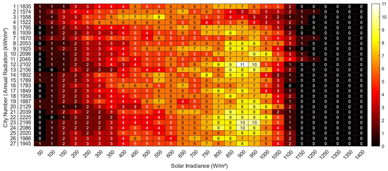
Table 6 presents the irradiance distribution for a typical year in each Brazilian capital. Each column represents the final range of irradiance values analyzed, with the initial value being that of the previous column. From all cities, on average, 35% of annual irradiation results in irradiance levels between 700 and 900 W/m² (columns from 750 to 950 in Table 6), with cities 12, 22, 23, and 24 having values above 40% for the same interval. Furthermore, around 2% of annual irradiation is due to irradiances above 1,000 W/m², the standard test value for photovoltaic modules.

In systems with ILR > 1, one should expect power limitation in the inverters for high irradiance levels above 1,000 W/m². Despite this, the loss due to limitation in one year may not be significant if the frequency of occurrences of these irradiance levels is low.

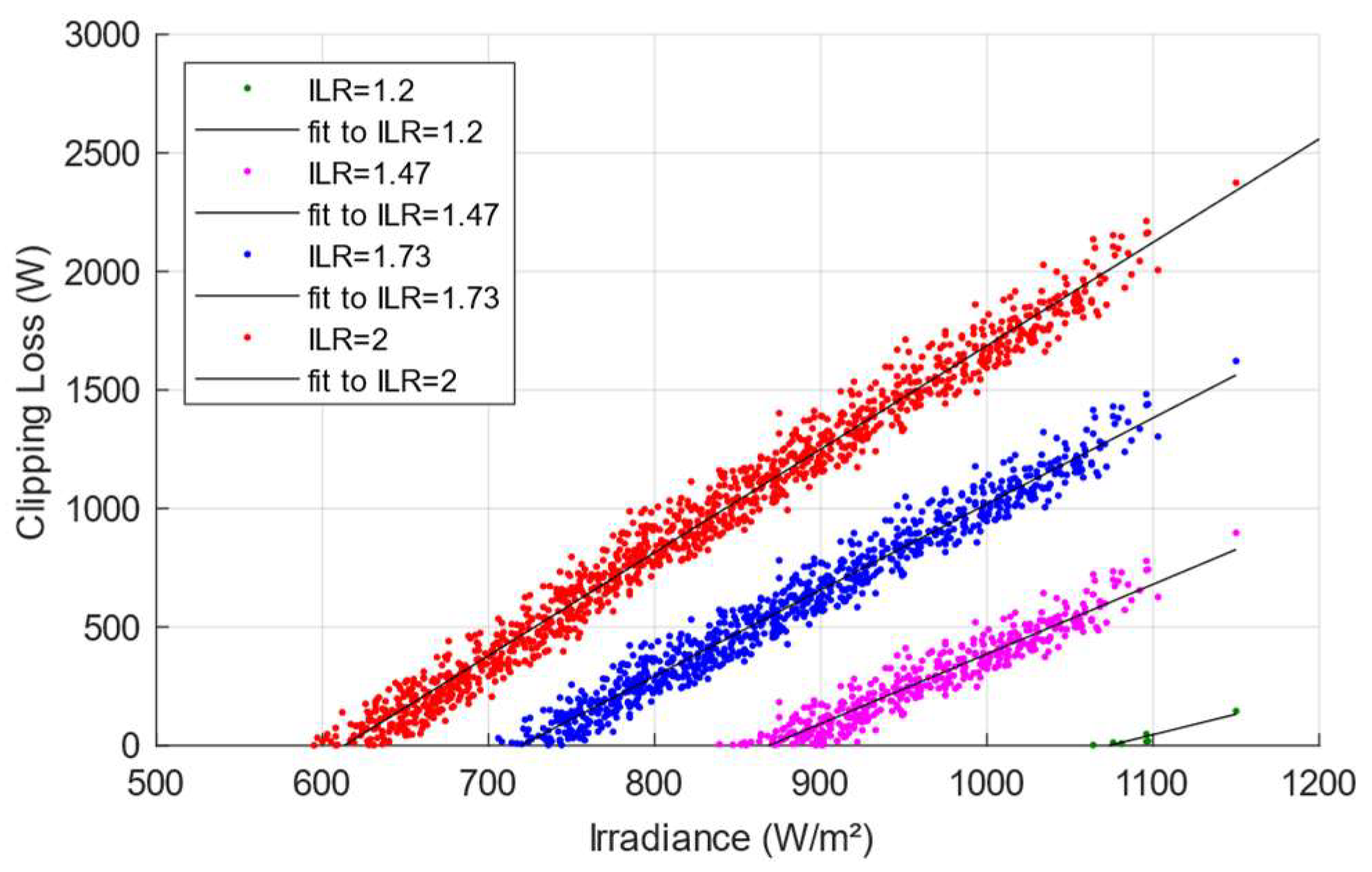
Inverter 1 (3 kW) installed in city 1 (Aracajú) is used to illustrate the main concepts. Some specific cases of limitation begin to be observed for ILR equal to 1.15 once the solar irradiance above 1,000 W/m² does not currently occur. Figure 1 shows some cases of power limitations for different ILRs. As expected, the higher the irradiance, the greater the limited power, and the larger the generator, the lower the irradiance required for the limitation to begin.

There is not even a single irradiance value for which the limitation begins, but rather a range of values that depend on the factors that impact the power delivered by the photovoltaic modules. For the case of ILR equal to 1.47 in Table 6, it is observed that power limitation can start between 840 W/m² and 922 W/m².

The main impact factors of this limitation are cell temperature and degradation due to module aging and losses up to the inverter input terminals.

Considering mono/polycrystalline silicon PV modules, the power delivered by the generator reduces increasing temperature, and the same occurs with increasing aging. Consequently, the inverter will not have the same power levels at its input, thus reducing the limited power.

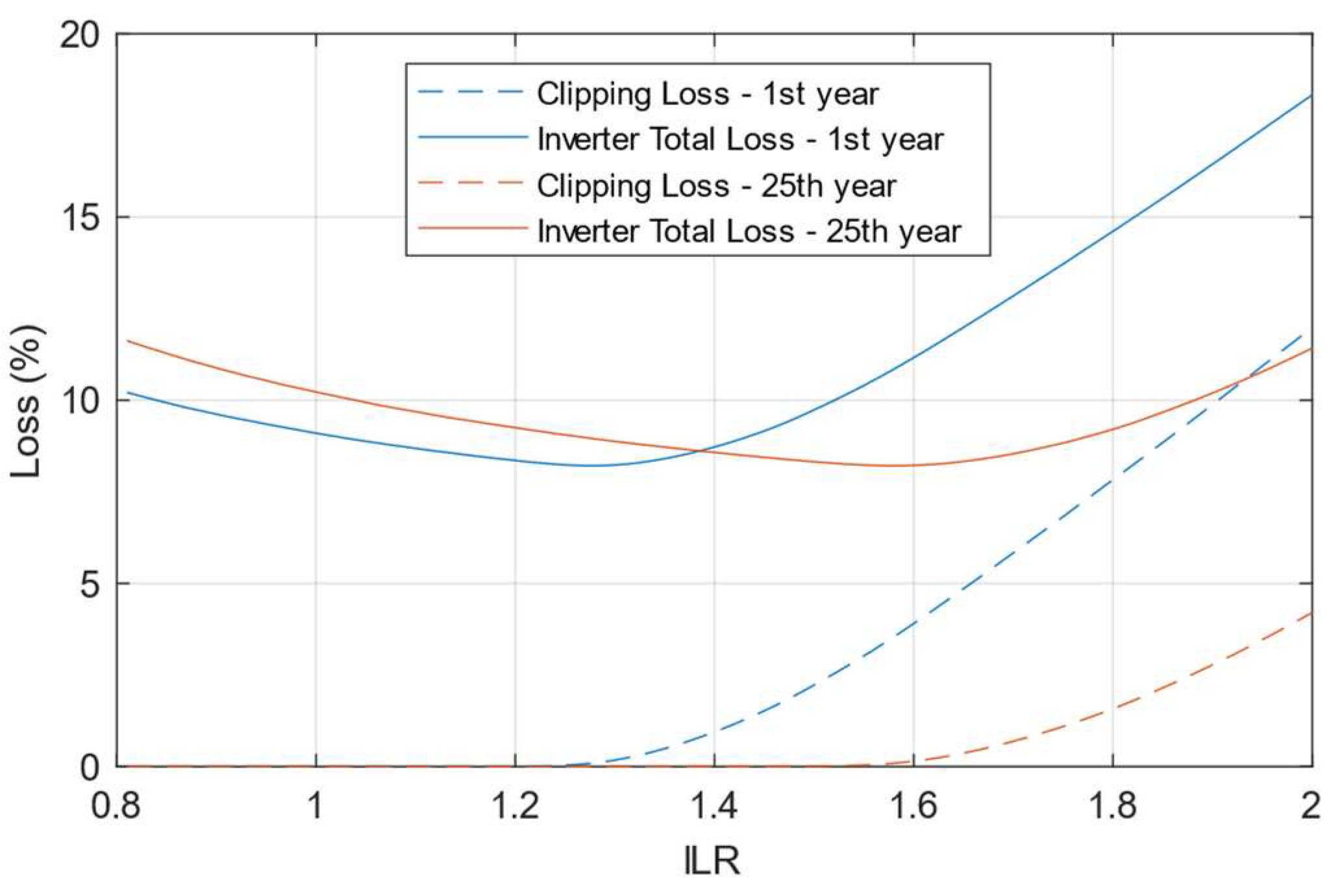
In the specific case of aging, the system with an ILR of 1.47 failed to use around 1.8% of the energy at the inverter input in the first year of operation (Figure 2). In the 25th year, this percentage became practically zero. In the first year, the loss percentage due to clipping starts to be significant for an ILR of 1.25; in the 25th year, it becomes significant for an ILR of 1.55.

The loss due to clipping is the difference between the maximum theoretical power at the inverter input and its actual conditioning capability. For example, considering the first year of operation (Figure 3), an ILR equal to 1.6 relates to an inverter clipping loss of around 3.9%, Equation (19), and the total is 11.2%, Equation (20). On the other hand, when the value is below 1.2, it is insignificant. Over the years, the inverter clipping loss has reduced to 0.15% and the total to 8.2% due to PV module aging effects negatively impacting its power.

$${Clipping\_Loss}_{\%}=100·{\displaystyle \frac{\int Clipping\_Loss\left(t\right)dt}{\int P_m\left(t\right)·\left(1-{DC\_Losses}_{\%}\right)dt}}$$

(19)

$${Inverter\_Total\_Loss}_{\%}=100·{\displaystyle \frac{\int Inverter\_Total\_Loss\left(t\right)dt}{\int P_m\left(t\right)·\left(1-{DC\_Losses}_{\%}\right)dt}}$$

(20)

where ${DC\_Losses}_{\mathrm{\%}}$, Equation (21), accounts for the aggregated losses impact on the maximum PV power generated: $L_{so}$ is the Soiling Loss; $L_{mi}$ is the Mismatch Loss; $L_{df}$ is the Degradation Loss factor; and $L_{arw}$ is the Array Ohmic Wiring Loss.

$${DC\_Losses}_{\%}=1-(1-L_{so})·(1-L_{mi})·(1-L_{df})·(1-L_{arw})$$

(21)

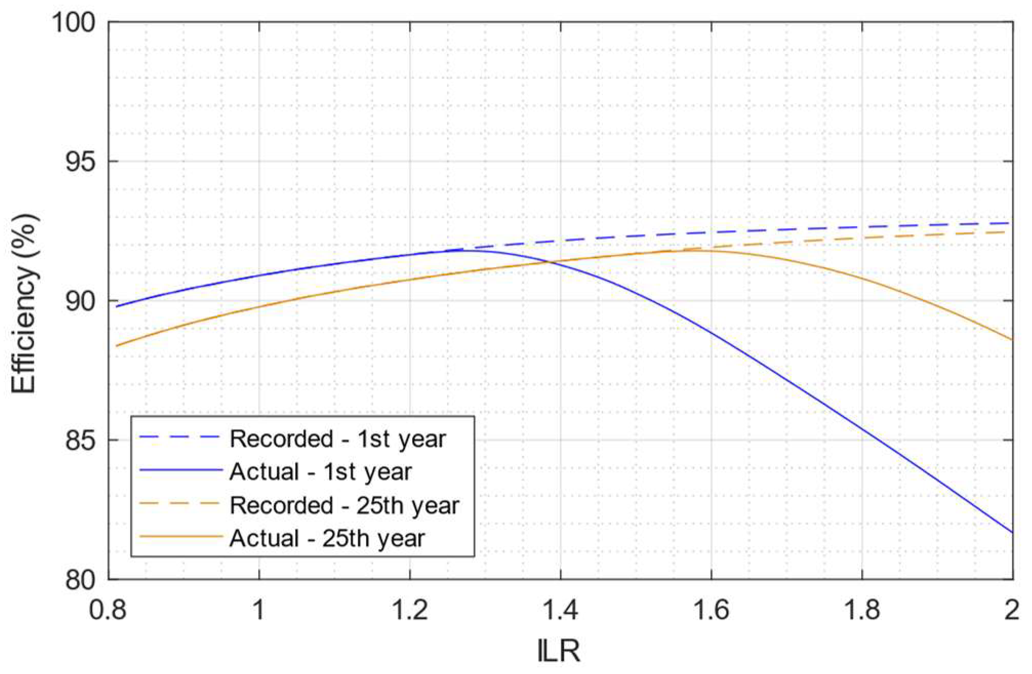
The incapacity of the inverter to condition all power incurs losses beyond the typical DC/AC conversion losses. It prompts the need to evaluate the system's efficiency from two distinct perspectives: recorded and actual efficiency. Recorded efficiency reflects the performance of the equipment and never accounts for the available power over the inverter capacity. However, actual efficiency depicts the operational reality and is thus more relevant from a practical standpoint.

The dashed curves in Figure 4 represent the recorded efficiencies in a year, accounting only for the typical DC/AC conversion losses. It shows an efficiency increase with the ILR and tends to values close to 92.5%. However, the operational reality is masked by disregarding the inverter's inability to condition all available power. The solid curves in Figure 4 represent the actual efficiencies, which move away from the dashed ones as the limited energy increases, being 81.7% and 88.6% for ILR = 2 in the first and 25th year, respectively.

The peaks of the actual efficiency curves (Figure 4) are 91.8%, and in the 1st year of operation, the occurrence occurs for ILR = 1.28, and for the 25th year for ILR = 1.58, that is, the curve shifts towards the right over time. In practice, the ILR remains fixed, and if it is lower than the ILR at the point of intersection of the continuous curves (1.39), then a reduction in the actual efficiency of the inverter will be observed over the years; otherwise, an increase in the actual efficiency.

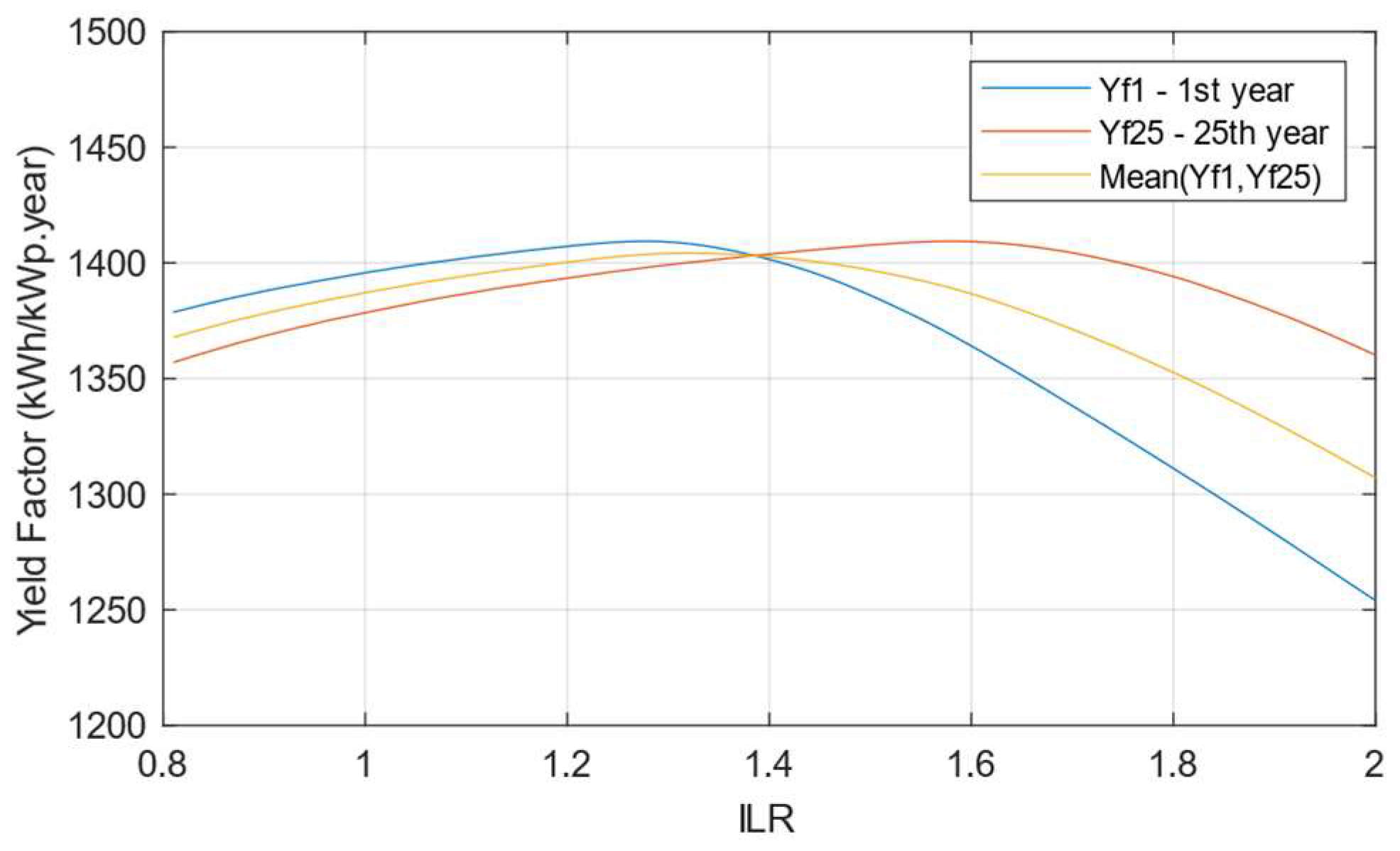
The Final Yield of a photovoltaic system is directly related to the energy delivered to the distribution network. Most losses up to the point of delivery are represented by a linear relationship except for losses in the inverter. Therefore, the Final Yield curve has the same shape as the actual efficiency curve (Figure 5), and the analyses are analogous to those already carried out. It should only be noted that the maximum Final Yield is 1,409 kWh/kWp.year.

When defining the ILR at the design stage, choosing it within a range of values encompassing the maximum Final Yield and observing its variability over time is reasonable. It is also a fact that the greater the photovoltaic generator, the greater the use of hours of sunlight. Therefore, the energy generated is more significant, often leading to choosing high ILR values, even with high losses due to clipping.

Hence, it is evident from Figure 5 that the oversizing strategy is constrained not only by the maximum input current and voltage of the inverter but also by the yearly optimal ILR, wherein the Final Yield experiences a significant change over time to a fixed ILR.

On the other hand, the system's financial investment also increases with the ILR; that is, the cost concerning the AC side (inverter, cables, and protections) remains the same, while the cost of the DC side (photovoltaic modules, cables, and protections mainly) increases with the ILR. The relative cost per power unit (R$/kWp) is reduced when the purchase volume increases, Which is already accounted for in the Greener database [32].

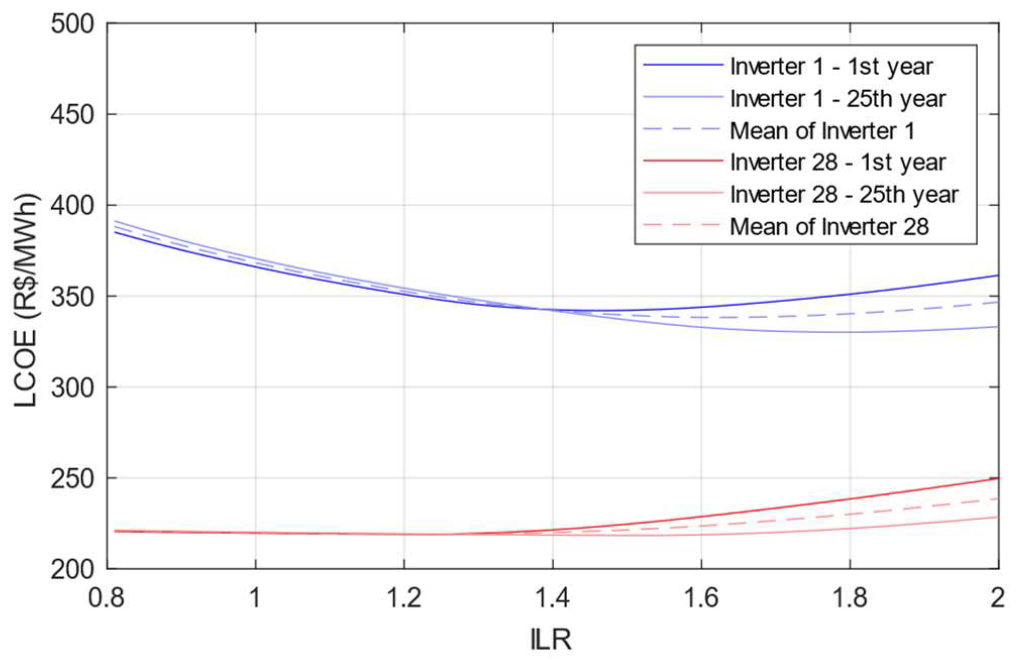
By applying the relative cost in (18) and dividing the result by the Final Yield, the LCOE is obtained. Lower power inverters tend to have higher LCOE than higher power ones, Figure 6. Irrespective of inverter nominal power, a notable minimum disparity exists between the LCOE values observed in the first and 25th years for the inverter, provided the ILR is lower than that of the curve intersection point, as depicted in Figure 6. Even for inverter 28, the intersection point exists at an ILR of 1.25. Conversely, when ILR exceeds this intersection point, a trend emerges wherein LCOE decreases over time while the ILR increases.

It is essential to acknowledge that efficiency curves play a crucial role in shaping the Final Yield, which also holds for LCOE curves. Increased losses invariably elevate the LCOE. Inverters with lower power ratings typically exhibit a steeper curve inclination before the intersection point, indicative of higher losses attributed to lower DC power levels. This is particularly evident for inverter 1, characterized by its lower efficiency curve.

Examining both the LCOE and the Final Yield reveals that the optimal ILR varies for each, shifting over time, thus complicating the search for an ideal solution. Even if such an optimal ILR can be identified, it is essential to evaluate whether the effort invested in finding it is justified. Notably, practical scenarios are constrained by limitations imposed by input inverters, which restrict array size based on current and voltage thresholds. Furthermore, operational efficiency depends on maintaining the power supply within a specific MPPT voltage range. Consequently, the effective ILR range often proves to be narrower than that simulated in this study.

Another constraint arises from the necessity of employing nearly identical photovoltaic modules, particularly within each MPPT channel. Consequently, this requirement yields discrete ILR values within the appropriate range, limiting available options. For instance, inverter 1 offers only four ILR selections: {1.07, 1.20, 1.33, 1.47}. As a result, the optimal ILR point is often more theoretical than practical, with the likelihood of it not being present in real-world applications.

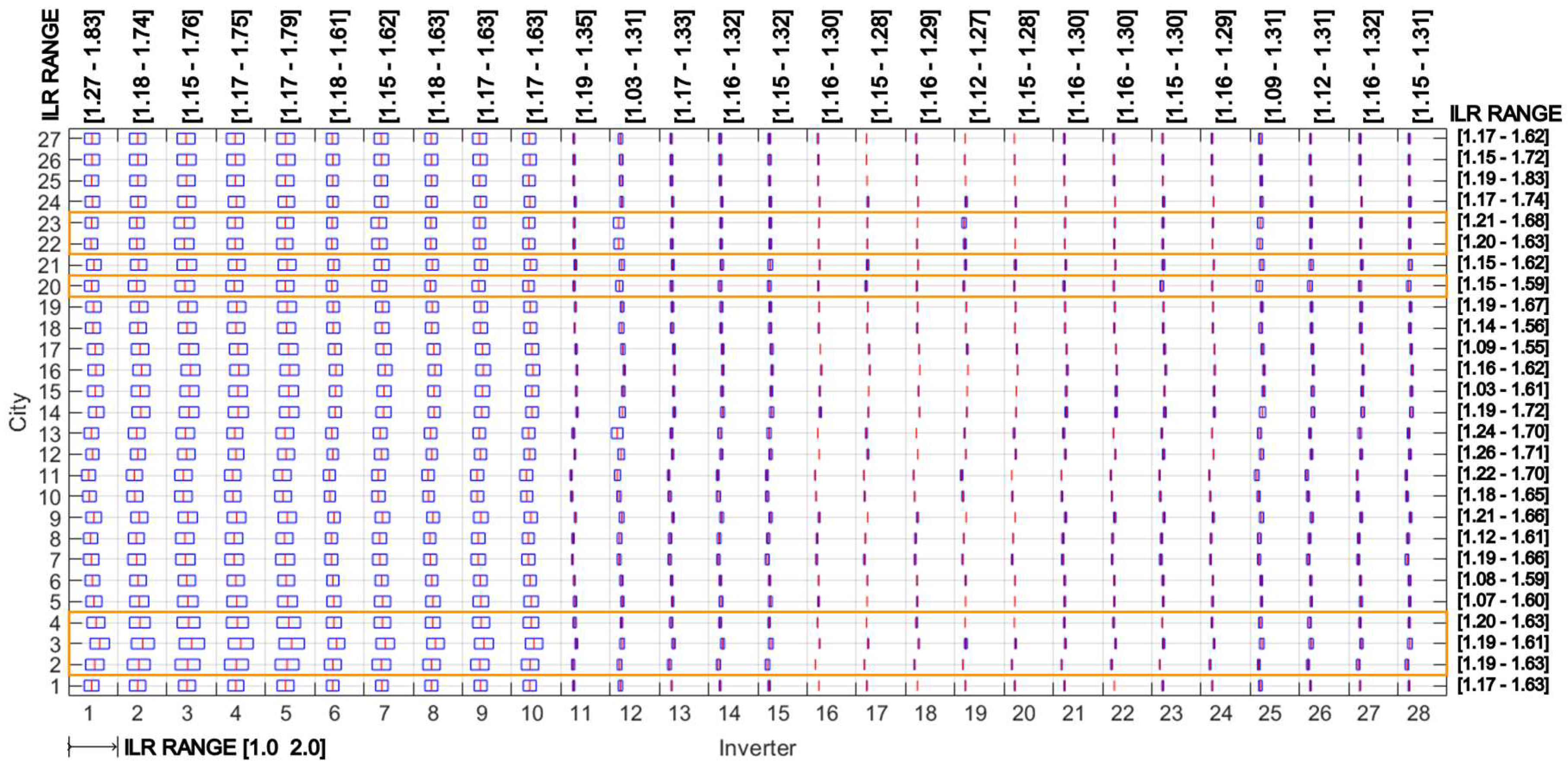
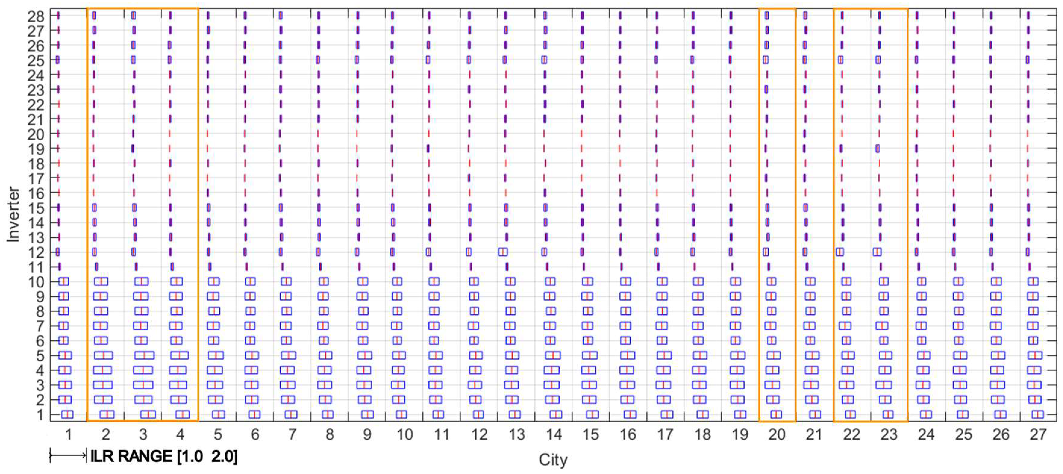
A pragmatic strategy should involve determining ILR ranges to enhance the probability of identifying a feasible ILR. One viable approach is delineating the range between the minimum LCOE and the maximum Final Yield, ensuring satisfactory performance across both objectives. Nevertheless, it is essential to note that each pairing of inverter and city will yield a distinct ILR range.

The ILR ranges for each city and inverter are displayed in Figure 8 and Figure 9. In this study, twenty-seven inverters have high efficiency, while only Inverter 1 has a low-efficiency curve (Figure 1). When we compared its ILR range behavior with others with equal nominal power inverters (2 to 5), we noticed that it shifted the range to the right (Figure 9); this suggests that more PV power is needed to compensate for the Inverter 1 losses.

Notably, inverters 1 to 10, which have nominal powers of 3 kW and 5 kW, exhibit broader ranges than others. Given that the system costs are the same in all cities and each city has high irradiance, and assuming that the efficiency curves of each inverter are similar to each other (except for inverter 1), the optimal ILR range is mainly affected by the nominal power in modern inverters; as the nominal power increases, the maximum ILR in the optimal range tends to decrease.

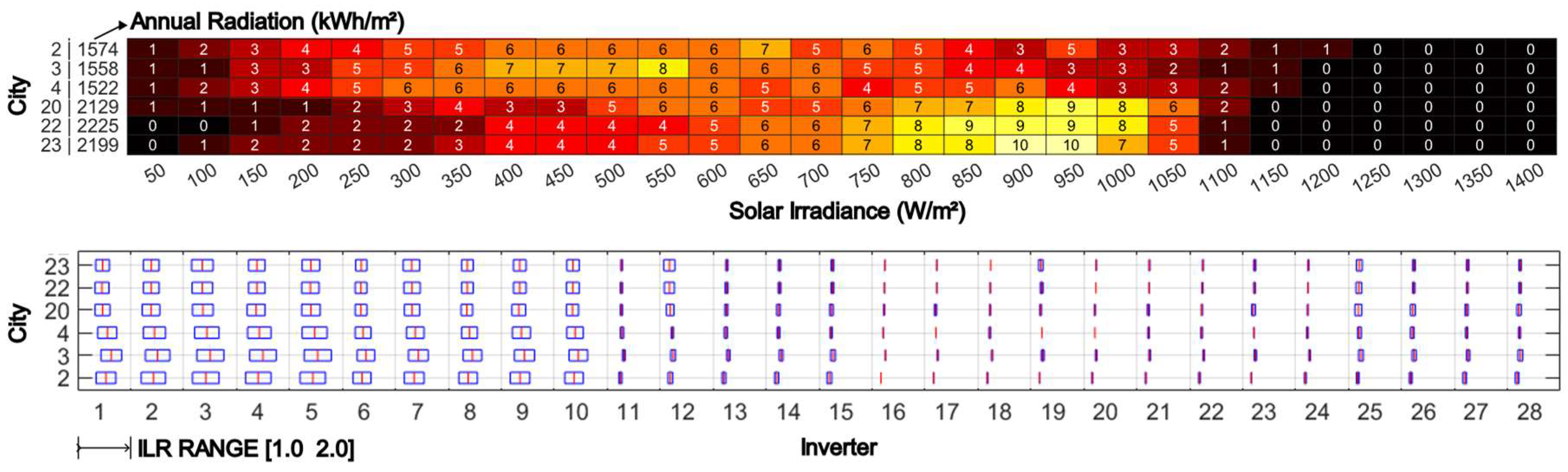
In the analysis of extreme irradiation scenarios, it was observed that cities 2, 3, and 4 exhibited the lowest irradiance values, while cities 20, 22, and 23 had the highest (Figure 7).

Figure 7. Summary of Table 6 and Figure 8 for three high- and low-irradiation cities, referred to respectively as [20, 22, and 23] and [2, 3, and 4].

Figure 7. Summary of Table 6 and Figure 8 for three high- and low-irradiation cities, referred to respectively as [20, 22, and 23] and [2, 3, and 4].

When considering middle and high-power inverters (ranging from 11 to 28), the differences in ILR ranges were minimal. However, for low-power inverters (ranging from 1 to 10), the ILR range showed significant variability between high- and low-irradiation cities. This difference can be attributed to the combined effects of the expected irradiance levels in each city throughout the year and the efficiency characteristics of the inverters. In high-irradiation cities, where the expected irradiance levels fall between 800 to 950 W/m² (Figure 7), the inverters operate within a high-efficiency region, leading to similar ILR ranges. In contrast, low-irradiation cities experience a wider range of irradiance below 750 W/m², and the nonlinearity of the inverter's efficiency curve has a more pronounced impact on the variability of ILR ranges between cities (Figure 7). Additionally, these cities have higher ILR ranges than high-irradiation cities (Figure 9).

Figure 8. Exploring the inverter's ILRs for each city between the ILRs that maximize the Final Yield and minimize the LCOE. Mean Final Yield and LCOE curves from the first and 25th years were used. Obs.: This plot is not a statistical boxplot. Its purpose is to compare the ILR ranges defined by minimum LCOE and maximum Final Yield.

Figure 8. Exploring the inverter's ILRs for each city between the ILRs that maximize the Final Yield and minimize the LCOE. Mean Final Yield and LCOE curves from the first and 25th years were used. Obs.: This plot is not a statistical boxplot. Its purpose is to compare the ILR ranges defined by minimum LCOE and maximum Final Yield.

Figure 9. Plot switching the axes from Figure 8. Obs.: This plot is not a statistical boxplot. Its purpose is to compare the ILR ranges defined by minimum LCOE and maximum Final Yield.

Figure 9. Plot switching the axes from Figure 8. Obs.: This plot is not a statistical boxplot. Its purpose is to compare the ILR ranges defined by minimum LCOE and maximum Final Yield.

The strong relationship between irradiance level and temperature creates a complex interaction when assessing the ILR, making it challenging to attribute changes in the ILR solely to irradiance. Additionally, various technical and economic factors may also contribute to this interaction. They may also have counteractions between them, making the definition of ILR less straightforward and necessitating thorough analysis to define a reasonable ILR range. A wider range of ILR increases the likelihood of finding viable solutions, while a narrower focus may limit practical implementation options. This approach is not exhaustive and may benefit from complementation to encompass a broader spectrum of solutions.

5. Conclusions

Evaluating solar resources across Brazilian capitals has been done, utilizing data from the Brazilian Solar Energy Atlas validated by meteorological stations. The analysis has provided valuable insights into the potential of solar energy generation in various regions.

Key findings include identifying power limitations in systems with Inverter Load Ratio (ILR) values above 1, particularly concerning high irradiance levels exceeding 1,000 W/m². Although power limitations may occur, their impact on energy loss may not be significant if high irradiance levels are infrequent.

Moreover, the study elucidates the complexities associated with inverter efficiency and Final Yield in relation to ILR values. Practical considerations, such as reference ILRs, ignore the challenges of selecting an ILR for real-world applications, which must be used only in initial studies.

Establishing ranges between the ILR that minimizes LCOE and the one that maximizes Final Yield is a key strategy for effectively identifying feasible ILR values. By observing the curves and their evolution over time, the designer can expand this range by considering a tolerance of energy loss, which would increase the flexibility. In all cases, it is essential to recognize the variability in ILR ranges across different inverter-city pairings when comparing ILRs for different inverters and cities. This is a crucial insight revealed by the analysis.

The optimal ILR range for medium and high-power modern inverters in Brazilian capitals was between 1.1 and 1.3. However, for low-power inverters, the range was extended to 1.8. The ILR range was discovered for a specific tilt facing North. This approach can be applied to analyze various arrays to assess different tilts and orientations or even combinations when utilizing inverters with multiple Maximum Power Point Tracking (MPPTs). In less favorable generation scenarios, the ILR can exceed 2.

When installing solar power systems, the type of mounting structure chosen can significantly affect initial costs. For instance, a solar tracker solution can boost the Final Yield but also involves higher capital costs and maintenance. Careful logistics planning between sites is also crucial in large countries like Brazil.

Upon further analysis, it can be inferred that the optimal range of the ILR has become more responsive to the power capacity of inverters. This trend emerged as technology advanced, resulting from a converging efficiency curve among manufacturers.

While this study provides valuable insights, it also acknowledges its limitations. It suggests further research to explore complementary approaches for optimizing ILR selection and maximizing solar energy generation efficiency. The tool would be improved by incorporating probabilistic scenarios and Monte Carlo evaluations. Additionally, it would be beneficial to change the financial metric to Value-Adjusted Levelized Cost of Electricity (VALCOE) to accurately represent the economic value of the power plant based on its capacity, flexibility, and electricity cost. Another possible method to consider is incorporating the required area for each generator and factoring in the land cost.

Furthermore, enhancing the accuracy of the tool results can be achieved by incorporating high-resolution meteorological data and exploring alternative power output models for PV generators that account for variables such as wind speed. Additionally, it would be advantageous to integrate power output models for inverters that consider multiple maximum power point tracking (MPPT) and efficiency curves.